Reduced-Order Neural Network Synthesis with Robustness Guarantees

Abstract

In the wake of the explosive growth in smartphones and cyberphysical systems, there has been an accelerating shift in how data is generated away from centralised data towards on-device generated data. In response, machine learning algorithms are being adapted to run locally on board, potentially hardware limited, devices to improve user privacy, reduce latency and be more energy efficient. However, our understanding of how these device orientated algorithms behave and should be trained is still fairly limited. To address this issue, a method to automatically synthesize reduced-order neural networks (having fewer neurons) approximating the input/output mapping of a larger one is introduced. The reduced-order neural network’s weights and biases are generated from a convex semi-definite programme that minimises the worst-case approximation error with respect to the larger network. Worst-case bounds for this approximation error are obtained and the approach can be applied to a wide variety of neural networks architectures. What differentiates the proposed approach to existing methods for generating small neural networks, e.g. pruning, is the inclusion of the worst-case approximation error directly within the training cost function, which should add robustness to out-of-sample data-points. Numerical examples highlight the potential of the proposed approach. The overriding goal of this paper is to generalise recent results in the robustness analysis of neural networks to a robust synthesis problem for their weights and biases.

I Introduction

As smartphones get increasingly integrated into our daily lives and the numbers of both cyberphysical systems and smart devices continues to grow, there has been a noticeable evolution in the way many large data sets are being generated. In fact, Cisco [cisco] predicted that in 2021, whilst 20.6 ZB of data (e.g. large ecommerce site records) will be handled by cloud-based approaches in large data-centres, this amount will be dwarfed by the 850 ZB generated by local devices [zhou]. In response to data sources becoming more device-centric, there has been a shift in focus for many machine learning algorithms towards both implementing and training them locally on (potentially hardware limited) devices. Running the algorithms on the devices represents a radical shift away from traditional centralised learning where the data and algorithms are stored and processed in the cloud but, as described in [zhou], brings the benefits of i) increased user privacy as the data is not transmitted to a centralised sever ii) reduced latency since the algorithms can react immediately to newly generated data from the device and iii) improved energy efficiency mostly because the data and algorithm outputs don’t have to be constantly transferred to and from the cloud. However, running algorithms locally on devices brings its own issues, most notably in dealing with the devices’ limited computational power, memory and energy storage. Overcoming these hardware constraints has motivated substantial efforts on improving algorithm design, particularly towards developing leaner, more efficient neural networks [sze].

Two popular approaches to make neural network algorithms leaner and more hardware-conscious are i) quantised neural networks [quant1, quant2, quant3], where fixed-point arithmetic is used to accelerate the computational speed and reduce memory footprint, and ii) pruned neural networks [liu2018rethinking, prune_state, janowsky, karnin, mozer1, mozer2, lecun, hassibi, gale, lee, lin, han, molchanov, li2016], where, typically, the weights contributing least to the function mapping are removed, promoting sparsity in the weights. Both of these approaches have achieved impressive results. For instance, by quantising, [lin2016fixed] was able to reduce model size by $>20\%$ without any noticeable loss in accuracy when evaluated on the CIFAR-10 benchmark and [han2015learning] demonstrated that between 50-80$\%$ of its model weights could be pruned with little impact on performance [sze]. However, our understanding of neural network reduction methods such as these remains lacking and reliably predicting their performance remains a challenge. Illustrating this point, [liu2018rethinking] stated that for pruned neural networks “our results suggest the need for more careful baseline evaluations in future research on structured pruning methods” with a similar sentiment raised in [prune_state] “our clearest finding is that the community suffers from a lack of standardized benchmarks and metrics”. These quotes indicate a need for robust evaluation methods for lean neural network designs, a perspective explored in this work.

Contribution

This paper introduces a method to automatically synthesize neural networks of reduced dimensions (meaning fewer neurons) from a trained larger one, as illustrated in Figure 1. These smaller networks are termed reduced-order neural networks since the approach was inspired by reduced order modelling in control theory [glover_modred]. The weights and biases of the reduced order network are generated from the solution of a semi-definite program (SDP)- a class of well-studied convex problems [boyd] combining a linear cost function with a linear matrix inequality (LMI) constraint- which minimises the worst-case approximation error with respect to the larger network. Bounds are also obtained for this worst-case approximation error and so the performance of the network reduction is guaranteed. In this way, the method is said to be “robust” as it ensures the approximation error of the reduced-order neural network remains bounded for all input data in certain pre-defined sets, in a manner specified by the bound of Theorem 1.

What separates the proposed synthesis approach to the existing methods for generating efficient neural networks, e.g. pruning, is the inclusion of the worst-case approximation error of the reduced-order neural network directly within the cost function for computing the weights and biases. It is expected that this approach should offer two main advantages over classical pruning methods:

1. The method is robust in the sense that it provides guarantees of the approximation error with respect to the full-order network, unlike with pruning.

2. The method is one of the first to do automatic neural network synthesis from the solution of a robust optimisation problem, with the weights and biases of the reduced-order neural networks generated in one-shot by solving a convex semi-definite program. Besides being of theoretical interest as an alternative to training via backpropogation, the main advantage of this approach is that it allows the worst-case error to be included directly within the training cost function which may result in out-of-sample generality in worst-case settings.

Whilst the presented results are still preliminary, their focus on robust neural network synthesis introduces a new set of of tools to generate lean neural networks which should have more reliable out-of-sample performance, and which are equipped with approximation error bounds. The broader goals of this work are to translate recent results on the verification of NN robustness using SDPs [pappas, raghunathan] into a synthesis problem, mimicking the progression from absolute stability theory [zames] to robust control synthesis [doyle] witnessed in control theory during the 1980s. In this way, this work carries on the tradition of control theorists exploring the connections between robust control theory and neural networks, as witnessed since the 1990s with Glover [chu], Barabanov [barabanov], Angeli [angeli] and Narendra [narendra].

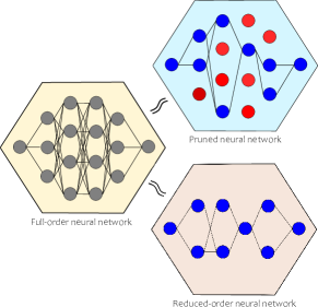
Figure 1: Illustration of two different approximations of a neural network (termed the full-order network) to enable it to be run on limited hardware. One approach is to use network pruning to make the weights sparse while the second is to develop a reduced-order network with fewer neurons. This paper proposes a method to synthesize the weights and biases of the reduced order network such that they robustly minimise the approximation error with respect to the full order network.

I-A Notation

Non-negative real vectors of dimension $n$ are denoted $\mathbb{R}^{n}_{+}$. A positive (negative) definite matrix $\Omega$ is denoted $\Omega\succ(\prec)~{}0$. Non-negative diagonal matrices of dimension $n\times n$ are $\mathbb{D}^{n}_{+}$. The matrix of zeros of dimension $n\times m$ is $\bm{0}_{n\times m}$ and the vector of zeros of dimension $n$ is $\bm{0}_{n}$. The identity matrix of size $n$ is $I_{n}$. The vector of 1s of dimension $n$ is $\bm{1}_{n}$ and the $n\times m$ matrix of 1s is $\bm{1}_{n\times m}$. The $i^{\text{th}}$ element of a vector $x$ is denoted $x_{i}$ unless otherwise defined in the text. The $\star$ notation is adopted to represent symmetric matrices in a compact form, e.g.

$$\begin{bmatrix}A&B\\ B^{T}&C\end{bmatrix}=\begin{bmatrix}A&B\\ \star&C\end{bmatrix}.$$ (1)

I-B Neural networks

The neural networks considered will be treated as functions $f(x):\mathcal{X}\to\mathcal{F}$ mapping input vectors of size $x\in\mathbb{R}^{n_{x}}$ to output vectors of dimension $f(x)\in\mathbb{R}^{n_{f}}$. In a slight abuse of notation, $\phi(\cdot):\mathbb{R}^{n_{k}}\to\mathbb{R}^{n_{k}}$ will refer to mappings of both scalars and vectors, with the vector operation applied element-wise. The full-order neural network will be composed of $l$ hidden layers, with the $k^{\text{th}}$ layer being composed of $n_{k}$ neurons. The total number of neurons in the full-order neural network is $N=\sum_{k=1}^{l}n_{k}$. Similarly, the reduced-order neural network will be composed of $\lambda$ hidden layers with the $k^{\text{th}}$ layer being composed of $m_{k}$ neurons. The total number of neurons in the reduced-order network is $M=\sum_{k=1}^{\lambda}m_{k}$. The dimension of the domain of the activation functions is defined as $\bar{N}=N-n_{l}+n_{x}$ (full-order network) and $\bar{M}=M-n_{\lambda}+n_{x}$ (reduced-order network).

II Problem statement

In this section, the general problem of synthesizing reduced-order NNs is posed. Consider a nonlinear function $f(x):\mathcal{X}\to\mathcal{F}$ mapping input data $x\in\mathcal{X}$ to an output set $\mathcal{F}$. The goal of this work is to generate a “simpler” function $g(x):\mathcal{X}\to\mathcal{G}$ that is as “close” as possible to $f(x)$ for all $x\in\mathcal{X}$. Here, “simpler” will refer to the dimension of the reduced-order neural network’s weight matrix being smaller than the full-order one and “close”-ness relates to the approximation error between the two functions $f(x)$ and $g(x)$ measured by the induced 2-norm $\sup_{x\in\mathcal{X}}\|f(x)-g(x)\|_{2}$. The goal is to automatically synthesize the simpler functions $g(x)$ from the solution of a convex problem and obtain worst-case bounds for approximation error with respect to the larger neural network $f(x)$ for all $x\in\mathcal{X}$.

To ensure that the function approximation problem remains feasible, structure is added to the set $\mathcal{F}$. It is assumed that the function being approximated $f(x)$ is generated by a feed-forward neural network

$$x^{0} =x,$$ (2a)

$$x^{k+1} =\phi(W^{k}x^{k}+b^{k}),\quad k=0,1,\dots,l-1,$$ (2b)

$$f(x) =W^{l}x^{l}+b^{l}.$$ (2c)

Here, the input data $x^{0}=x\in\mathcal{X}\subseteq\mathbb{R}^{n_{x}}$ is mapped through the nonlinear activation functions $\phi(\cdot)$ (which could be the standard choices of ReLU, sigmoid, tanh or any function that satisfies a quadratic constraint as given in Section III-B) element-wise with the weight matrices $W^{0}\in\mathbb{R}^{n_{1}\times n_{x}}$, $W^{k}\in\mathbb{R}^{n_{k+1}\times n_{k}}$ and biases $b^{k}\in\mathbb{R}^{n_{k+1}}$, $k=0,\,\dots,l-1$. Whilst the results are described for feed-forward neural networks, the method can be generalised to other network architectures, such as recurrent and even implicit neural networks [implicit]. As an aside, verifying the well-posedness of implicit neural networks has a strong connection to that of Lurie systems with feed-through terms [valmorbida].

The network (2) can be equivalently written in the implicit form

$$\check{x} =\phi(W\check{x}+W_{0}x+b),\quad\quad\phi(.):~{}\mathbb{R}^{N}\mapsto\mathbb{R}^{N},$$ (3a)

$$f(x) =W^{f}\check{x}+b^{l},$$ (3b)

where

$$\check{x} =\begin{bmatrix}x^{1}\\ x^{2}\\ \vdots\\ x^{l}\end{bmatrix},\,W=\begin{bmatrix}0&0&\ldots&0\\ W^{1}&\ddots&\ddots&\vdots\\ \vdots&\ddots&0&0\\ 0&\dots&W^{l-1}&0\end{bmatrix},\,W_{0}=\begin{bmatrix}W^{0}\\ 0\\ \vdots\\ 0\end{bmatrix},\,$$ (4a)

$$b =\begin{bmatrix}b^{0}\\ b^{1}\\ \vdots\\ b^{l-1}\end{bmatrix},\quad W^{f}=\begin{bmatrix}0,&\ldots\,,&0,&W^{l}\end{bmatrix}.$$ (4b)

The neural network $f(x)$ (which will be referred to as the full-order neural network) is to be approximated by another neural network $g(x)\in\mathcal{G}$ (referred to as the reduced-order neural network) of a smaller dimension

$$z^{0} =x,$$ (5a)

$$z^{k+1} =\phi\left(\sum_{i=0}^{\lambda-1}\Psi^{k+1,i}z^{i}+\beta^{k}\right),\quad k=0,1,\dots,\lambda-1,$$ (5b)

$$g(x) =\Psi^{\lambda}z^{\lambda}+\beta^{\lambda}.$$ (5c)

The weights and biases in this neural network are $\Psi^{k,i}\in\mathbb{R}^{m_{k+1}\times m_{i}}$, $\beta^{k}\in\mathbb{R}^{m_{k+1}}$, $k=0,\,\dots,\,\lambda-1$. The network structure in (5b) is general, and even allows for implicitly defined networks [implicit]. This generality follows from the lack of structure imposed on the matrices used in the synthesis procedure. However, by adding structure, the search can be limited to, for example, feed-forward networks, which are simpler to implement.

Similar to the full-order case, the network (5) can be written as

$$\check{z} =\phi({\Psi}\check{z}+\Psi_{0}x+\beta),\quad\phi(\cdot):\mathbb{R}^{M}\mapsto\mathbb{R}^{M},$$ (6a)

$$g =\Psi^{f}\check{z}+\beta^{\lambda},$$ (6b)

where

$$\check{z} =\begin{bmatrix}z^{1}\\ z^{2}\\ \vdots\\ z^{\lambda}\end{bmatrix},\,\Psi=\begin{bmatrix}\Psi^{1,1}&\Psi^{1,2}&\ldots&\Psi^{1,\lambda}\\ \Psi^{2,1}&\Psi^{2,2}&\ddots&\vdots\\ \vdots&\ddots&\ddots&\Psi^{\lambda-1,\lambda}\\ \Psi^{\lambda,1}&\dots&\Psi^{\lambda,\lambda-1}&\Psi^{\lambda,\lambda}\end{bmatrix},\,$$ (7a)

$$\Psi_{0} =\begin{bmatrix}\Psi^{1,0}\\ \Psi^{2,0}\\ \vdots\\ \Psi^{\lambda,0}\end{bmatrix},\,\beta=\begin{bmatrix}\beta^{0}\\ \beta^{1}\\ \vdots\\ \beta^{\lambda-1}\end{bmatrix},\,\Psi^{f}=\begin{bmatrix}0,&\ldots\,,&0,&\Psi^{\lambda}\end{bmatrix}.$$ (7b)

In this work, the dimension of the reduced-order network is fixed and the problem is to find the reduced-order NN’s parameters, being the weights $\Psi^{k,i}$ and biases $\beta^{k}$, that minimise the worst-case approximation error between the full and reduced order neural networks for all $x\in\mathcal{X}$. In practice, the dimension of the reduced-order network should be fixed to the minimum value for which Proposition 1 can be solved to give a sufficient level of performance, as typically increasing the dimension of this neural network should lead to improved approximations to the full-order one, as larger networks will be more expressive allowing them to more accurately approximate highly nonlinear functions. The main tool used for this reduced-order NN synthesis problem is the outer approximation of the NN’s input set $\mathcal{X}$, nonlinear activation function’s gains $\phi(\cdot)$ and the output error $f(x)-g(x)$ by quadratic constraints. These outer approximations enable the robust weight synthesis problem to be stated as a convex SDP, albeit at the expense of introducing conservatism into the analysis.

III Quadratic Constraints

In this section, the quadratic constraints for the convex outer approximations of the various sets of interest of the reduced NN synthesis problem are defined. These characterisations are posed in the framework of [pappas], which in turn was inspired by the integral quadratic constraint framework of [iqc] and the classical absolute stability results for Lurie systems [khalil].

III-A Quadratic constraint: Input set

The input data $x\in\mathcal{X}$ is restricted to the hyper-rectangle $\mathcal{X}_{\infty}$.

Definition 1

Define the hyper-rectangle $\mathcal{X}_{\infty}=\{x:\underline{x}_{i}\leq x_{i}\leq\overline{x}_{i},\,i=1,\,\dots,\,n_{x}\}$. If $x\in\mathcal{X}_{\infty}$ then $[x^{T}~{}1]P_{\mathcal{X}_{\infty}}[x^{T}~{}1]^{T}\geq 0$ where

$$P_{\mathcal{X}_{\infty}}=\begin{bmatrix}-\tau_{x_{\infty}}&\frac{\tau_{x_{\infty}}}{2}\left(\underline{x}+\overline{x}\right)\\ \star&-\underline{x}^{T}\tau_{x_{\infty}}\overline{x}\end{bmatrix},\quad\tau_{x_{\infty}}\in\mathbb{D}^{n_{x}}_{+}.$$ (8)

Note that the input set constraint characterised by Definition 1 can be equivalently written as

$$\omega(x)^{T}\Pi_{\infty}\omega(x)\geq 0$$ (9)

where

$$\Pi_{\infty}=\begin{bmatrix}-\tau_{x_{\infty}}&0_{n_{x}\times N}&0_{n_{x}\times M}&\frac{\tau_{x_{\infty}}}{2}\left(\underline{x}+\overline{x}\right)\\ \star&0_{N\times N}&0_{N\times M}&0_{N\times 1}\\ \star&\star&0_{M\times M}&0_{M\times 1}\\ \star&\star&\star&-\underline{x}^{T}\tau_{x_{\infty}}\overline{x}\end{bmatrix}$$

and

$$\mu(x)=\begin{bmatrix}x^{T}&\check{x}^{T}&\check{z}^{T}&1\end{bmatrix}^{T}.$$ (10)

III-B Quadratic constraint: Activation functions

The main obstacle to any robustness-type result for neural networks is accounting for the nonlinear activation functions $\phi(\cdot)$. To address this issue, the following function properties are introduced.

Definition 2

The activation function $\phi(s):\mathcal{S}\subset\mathbb{R}\to\mathbb{R}$ satisfying $\phi(0)=0$ is said to be sector bounded if

$$\frac{\phi(s)}{s}\in[0,\delta]\quad\forall s\in\mathcal{S},\quad\delta>0,$$ (11a)

and slope restricted if

$$\frac{d\phi(s)}{ds}\in[\underline{\beta},\beta],\quad\forall s\in\mathcal{S},\quad\beta>0.$$ (11b)

If $$\underline{\beta}=0 \phi(s) \phi(s)$$ then the nonlinearity is monotonic and if is slope restricted then it is also sector bounded. The activation function is bounded if

$$\phi(s)\in[\underline{c},\overline{c}],\quad\forall s\in\mathcal{S},$$ (11c)

it is positive if

$$\phi(s)\geq 0,\quad\forall s\in\mathcal{S},$$ (11d)

its complement is positive if

$$\phi(s)-s\geq 0,\quad\forall s\in\mathcal{S},$$ (11e)

and it satisfies the complementarity condition if

$$(\phi(s)-s)\phi(s)=0,\quad\forall s\in\mathcal{S}.$$ (11f)

Most popular activation functions, including the ReLU, (shifted-)sigmoid and tanh satisfy one or more of these conditions, as illustrated in Table I. As the number of properties satisfied by $\phi(\cdot)$ increases, the characterisation of this function within the robustness analysis improves, often resulting in less conservative results. It is also noted that to satisfy $\phi(0)=0$ some activation functions may require a shift, e.g. the sigmoid, or they may require transformations to satisfy additional function properties, as demonstrated in the representation of the LeakyReLU as a ReLU + linear term function.

$\phi(\cdot)$ property	Shifted sigmoid	tanh	ReLU	ELU
Sector bounded	✓	✓	✓	✓
Slope restricted	✓	✓	✓	✓
Bounded	✓	✓	×	×
Positive	×	×	✓	×
Positive complement	×	×	✓	×
Complementarity condition	×	×	✓	×

TABLE I: Properties of commonly used activation functions, including the sigmoid, tanh, rectified linear unit ReLU and exponential linear unit (ELU). The properties of other functions, such as the LeakyReLU, can also be inferred.

As is well-known from control theory [khalil], functions with these specific properties are important for robustness analysis problems because they can be characterised by quadratic constraints.

Lemma 1

Consider the vectors $y,y_{1}\in\mathbb{R}^{n_{y}}$, and $\upsilon\in\mathbb{R}^{n_{\upsilon}}$ that are mapped component-wise through the activation functions $\phi(\cdot):\mathbb{R}^{n_{y}}\to\mathbb{R}^{n_{y}}$ and $\tilde{\phi}(\cdot):\mathbb{R}^{n_{v}}\to\mathbb{R}^{n_{v}}$. If $\phi(y)$ is sector-bounded, then

$$(\delta y-\phi(y))^{T}{\bf T}^{\text{s}}\phi(y) \geq 0,\quad\forall y\in\mathbb{R}^{n_{y}},~{}{\bf T}^{\text{s}}\in\mathbb{D}^{n_{y}}_{+};$$ (12a)

slope-restricted then

$$\quad\quad\quad\forall\{y,\,y_{1}\}\in\mathbb{R}^{n_{y}},\,{\bf T}^{\text{sl}}\in\mathbb{D}^{n_{y}}_{+};$$ (12b)

bounded then

$$(\overline{c}-\phi(y))^{T}{\bf T}^{B}(\phi(y)-\underline{c}) \geq 0,\quad\forall y\in\mathbb{R}^{n_{y}},\,{\bf T}^{B}\in\mathbb{D}^{n_{y}}_{+};$$ (12c)

positive then

$$({\bf T}^{+})^{T}\phi(y)\geq 0,\quad\forall y\in\mathbb{R}^{n_{y}},\,{\bf T}^{+}\in\mathbb{R}_{+}^{n_{y}};$$ (12d)

such that is complement is positive then

$$({\bf T}^{c+})^{T}(\phi(y)-y)\geq 0,\quad\forall y\in\mathbb{R}^{n_{y}},\,{\bf T}^{c+}\in\mathbb{R}^{n_{y}}_{+}.$$ (12e)

If $$\phi(y)$$ satisfies the complementary condition then

$$(\phi(y)-y)^{T}{\bf T}^{0}\phi(y)=0,\quad\forall y\in\mathbb{R}^{n_{y}},\,{\bf T}^{0}\in\mathbb{D}^{n_{y}}.$$ (12f)

Additionally, if both $$\phi(y) \tilde{\phi}(\upsilon)$$ and and their complements are positive then so are the cross terms

$$\small\tilde{\phi}(\upsilon)^{T}{\bf T}^{\times}(\phi(y)-y)\geq 0,\;\forall\upsilon\in\mathbb{R}^{n_{v}},y\in\mathbb{R}^{n_{y}},\,{\bf T}^{\times}\in\mathbb{R}_{+}^{n_{\upsilon}\times n_{y}},$$ (12g)

$$\tilde{\phi}(\upsilon)^{T}{\bf T}^{\otimes}\phi(y)\geq 0,\;\forall\upsilon\in\mathbb{R}^{n_{v}},y\in\mathbb{R}^{n_{y}},\,{\bf T}^{\otimes}\in\mathbb{R}_{+}^{n_{\upsilon}\times n_{y}}.$$ (12h)

Inequalities (12a)-(12f) are well-known however the cross terms (12g)-(12h) acting jointly on activation function pairs are less so.

Remark 1

Lemma 1 is established globally, that is for all $y\in\mathbb{R}^{n_{y}}$. Some activation functions $\phi(\cdot)$ may be defined locally, or the sector, slope bounds may be tighter for restricted values of their arguments. In such cases, local versions of Lemma 1 may give less conservative results.   $\star$

The characterisation of the nonlinear activation functions via quadratic constraints allows the neural network robustness analysis to be posed as a SDP- with the various $\lambda$’s in Lemma 1 being decision variables. Such an approach has been used in [pappas, glover_modred, barabanov], and elsewhere, for neural networks robustness problems, with the conservatism of this approach coming from the obtained worst-case bounds holding for all nonlinearities satisfying the quadratic constraints. In this work, the aim is to extend this quadratic constraint framework for neural network robustness analysis problems to a synthesis problem.

A quadratic constraint characterisation of both the reduced and full-order neural networks can then be written, with the following lemma being the application of Lemma 1 for both the reduced and full-order neural networks.

Lemma 2

If the activation function $\phi(\cdot)$ satisfies one or more of the quadratic constraints of Lemma 1, then there exists a matrix

$$\Lambda=\begin{bmatrix}\bm{0}_{n_{x}\times n_{x}}&\Lambda_{12}&\Lambda_{13}&\Lambda_{14}\\ \star&\Lambda_{22}&\Lambda_{23}&\Lambda_{24}\\ \star&\star&\Lambda_{33}&\Lambda_{34}\\ \star&\star&\star&\Lambda_{44}\end{bmatrix},$$ (13)

defined by the ${\bf T}^{i}$’s ($i\in\left\{\text{s},\text{sl},+,c+,B,0,\times,\otimes\right\}$) of Lemma 1 such that

$$\mu(x)^{T}\Lambda\mu(x)\geq 0,\quad\forall x\in\mathcal{X}.$$ (14)

Proof:

The construction of $\Lambda$ for the sector nonlinearity associated with the full-order network is shown. Lemma 1 implies that for a matrix ${\bf T}^{\text{s}}\in\mathbb{R}^{N\times N}$

$$2\phi(\xi)^{T}{\bf T}^{\text{s}}(\xi-\phi(\xi))\geq 0$$

where, from equation (3), $\xi=W\check{x}+W_{0}x+b$. Noting that $\phi(\xi)=\check{x}$, expanding the above becomes

$$2\check{x}^{T}{\bf T}^{\text{s}}(W\check{x}+W_{0}x+b-\check{x})\geq 0$$

and majorising it gives

$$\begin{bmatrix}x\\ \check{x}\\ \check{z}\\ 1\end{bmatrix}^{T}\begin{bmatrix}0&W_{0}^{T}{\bf T}^{\text{s}}&0&0\\ \star&-2{\bf T}^{\text{s}}+{\bf T}^{\text{s}}W+W^{T}{\bf T}^{\text{s}}&0&{\bf T}^{\text{s}}b\\ \star&\star&0&0\\ \star&\star&\star&0\end{bmatrix}\begin{bmatrix}x\\ \check{x}\\ \check{z}\\ 1\end{bmatrix}\geq 0.$$ (15)

This clearly takes the form of the inequality in (14). All other cases are derived similarly.

Appendix 1 details the characterisation of $\Lambda$ for the specific case of the ReLU activation functions.

III-C Quadratic constraint: Approximation error of the reduced-order neural network

An upper bound for the approximation error between the full and reduced-order networks can also be expressed as a quadratic constraint. This error bound will be used as a performance metric to gauge how well the reduced-order neural network approximates the full-order one, as in how well $g(x)\approx f(x)~{}\forall x\in\mathcal{X}_{\infty}$.

Definition 3 (Approximation error)

For some $\gamma_{x}\geq 0$, $\gamma\geq 0$, the reduced-order NN’s approximation error is defined as the quadratic bound

$$\|f(x)-g(x)\|_{2}^{2}\leq\gamma_{x}\|x\|_{2}^{2}+\gamma,\quad\forall x\in\mathcal{X}_{\infty}.$$ (16)

In practice, this bound is computed by minimising over some weighted sum of $\gamma_{x}$ and $\gamma.$

Note that by using equations (3) and (6) the approximation error $f(x)-g(x)$ can be written as

$$f(x)-g(x)=L\mu(x)$$ (17)

where

$$\small L=\begin{bmatrix}0_{n_{f}\times n_{x}},&W^{f},&-\Psi^{f},&b^{l}-\beta^{\lambda}\end{bmatrix}$$ (18)

Similarly,

$$\gamma_{x}\|x\|_{2}^{2}+\gamma=\mu(x)^{T}\Gamma\mu(x)$$ (19)

where $\Gamma={\rm blockdiag}(\gamma_{x}I_{n_{x}},0_{N\times N},0_{M\times M},\gamma)$, so inequality (16) is equivalent to

$$\mu(x)^{T}(L^{T}L-\Gamma)\mu(x)\leq 0.$$

IV Reduced-order neural network synthesis problem

This section contains the main result of the paper; an SDP formulation of the reduced-order NN synthesis problem (Proposition 1). To arrive at this formulation, a general statement of the synthesis problem is first defined in Theorem 1. This theorem characterises the search for the reduced-order neural network’s parameters as minimising the worst-case approximation error for all inputs $x\in\mathcal{X}$.

Theorem 1

Assume the activation functions $\phi$ satisfy one or more of the properties from Definition 2. With fixed weights $\{w_{1},\,w_{2}\}\geq 0$, if there exists a solution to

$$\min_{\Psi,\,\Psi_{0},\,\Psi^{l},\,\beta,\,\beta^{\lambda},\,{\bf T}^{i},\,{\bf T}_{r}^{i},\tau_{x_{\infty}},\,\gamma_{x},\,\gamma} ~{}w_{1}\gamma_{x}+w_{2}\gamma,$$ (20a)

s.t.

$$\mu(x)^{T}\Pi_{\infty}\mu(x)+\mu(x)^{T}\Lambda\mu(x)+\mu(x)^{T}(L^{T}L-\Gamma)\mu(x)\leq 0,$$ (20b)

$$\gamma_{x}\geq 0,\,\gamma\geq 0,$$

then the worst-case approximation error is bounded by $\|f(x)-g(x)\|_{2}^{2}~{}\leq~{}\gamma_{x}~{}\|x\|_{2}^{2}~{}+~{}\gamma$ for all $x\in\mathcal{X}_{\infty}$.

Proof:

See Appendix 3.

The main issue with Theorem 1 is verifying inequality (20b) since it includes a non-convex bilinear matrix inequality (BMI) between the matrix variables of the reduced-order network’s weights, its biases and the scaling variables in $\Lambda$. The following proposition details how this constraint can be written (after the application of a convex relaxation of the underlying BMI) as an LMI. The search over the reduced NN variables can then be translated into a SDP, a class of well understood convex optimisation problems with many standard solvers such as MOSEK [mosek] implemented through the YALMIP [yalmip] interface in MATLAB or even the Robust Control Toolbox.

Proposition 1

Consider the full-order neural network of (2) mapping $x\to f(x)$ and the reduced-order neural network of (5) mapping $x\to g(x)$. For fixed weights $\{w_{1},\,w_{2}\}\geq 0$, if there exists matrix variables ${\bf T}^{i}$ (of appropriate dimension and property), ${\bf F}_{\Psi}\in\mathbb{R}^{M\times{M}},\,{{\bf F}_{0}}\in\mathbb{R}^{M\times n_{x}},\,{\bf F}_{\beta}\in\mathbb{R}^{M}$, $\Psi^{f}\in\mathbb{R}^{n_{f}\times M}$ and $\beta^{\lambda}\in\mathbb{R}^{n_{f}}$ that solve

$$\min_{{\bf F}_{\Psi},\,{\bf F}_{0},\,{\bf F}_{\beta},\,\Psi^{f},\,\beta^{\lambda},\,{\bf T}^{i},\,{\bf T}_{r}^{i},\tau_{x_{\infty}},\,\gamma_{x},\,\gamma}~{}w_{1}\gamma_{x}+w_{2}\gamma,$$ (21a)

$$\hskip 45.52458pt\text{s.t. }\quad\Omega_{\text{Schur}}\prec 0,\,\gamma_{x}\geq 0,\,\gamma\geq 0,$$ (21b)

with $\Omega_{\text{Schur}}$ defined in (LABEL:eq:schur) of Appendix 3, then the reduced-order network with weights and affine terms defined by

$$\Psi_{0}=U_{1}^{-1}{\bf F}_{0}\quad\Psi=U_{2}^{-1}{\bf F}_{\Psi}\quad\beta=U_{3}^{-1}{\bf F}_{\beta},$$ (22)

ensures that the worst-case approximation error bound of the reduced-order neural network satisfies $\|f(x)-g(x)\|_{2}^{2}~{}\leq~{}\gamma_{x}~{}\|x\|_{2}^{2}~{}+~{}\gamma$ for all $x\in\mathcal{X}_{\infty}$.