T-matrix method for calculation of second-harmonic generation in clusters of spherical particles

Abstract

In this article, we present a T-matrix method for numerical computation of second-harmonic generation from clusters of arbitrarily distributed spherical particles made of centrosymmetric optical materials. The electromagnetic fields at the fundamental and second-harmonic (SH) frequencies are expanded in series of vector spherical wave functions, and the single sphere T-matrix entries are computed by imposing field boundary conditions at the surface of the particles. Different from previous approaches, we compute the SH fields by taking into account both local surface and nonlocal bulk polarization sources, which allows one to accurately describe the generation of SH in arbitrary clusters of spherical particles. Our numerical method can be used to efficiently analyze clusters of spherical particles made of various optical materials, including metallic, dielectric, semiconductor, and polaritonic materials.

1 Introduction

Accurate description of light scattering from particles at the nanoscale has recently attracted growing interest from the electromagnetics and optics communities, chiefly owing to a plethora of applications made possible by our ability to control and manipulate light at this scale combined with rapid advances in nanofabrication techniques. In this context, a major rôle is played by localized surface plasmons, which are evanescent localized waves confined at the interface between metallic nanoparticles and the surrounding dielectric medium [1]. Indeed, at resonance, the excitation of localized surface plasmons is accompanied by the generation of strongly enhanced optical near-fields, a phenomenon that finds applications in many areas of science and engineering, including surface-enhanced Raman spectroscopy, optical nanoantennas and sensors, optical waveguides, metamaterials, and nonlinear optical microscopy [7, 8, 9, 10, 11, 4, 5, 6, 2, 3].

Second-harmonic generation (SHG) is a second-order nonlinear optical process in which an incident optical field oscillating at the fundamental frequency (FF), $\omega$, interacts with a nonlinear medium and gives rise to a scattered optical field oscillating at the second-harmonic (SH) frequency $\Omega=2\omega$ [12, 13, 14, 15]. There are two principal components of the nonlinear polarization, which are responsible for the SHG in so-called centrosymmetric media, that is media that are invariant to inversion symmetry transformations. The (local) surface nonlinear polarization is induced at the interface between the nanoparticle and the surrounding environment, within a thin region containing just a few atomic layers, and where the inversion symmetry is broken. The second component, the (nonlocal) bulk nonlinear polarization, depends on the derivatives of the optical field components at the FF inside the nonlinear scatterer. Second-harmonic radiation emitted from plasmonic nanoparticles is predominantly generated by surface nonlinear polarization sources, but in the case of dielectric nanoparticles surface and bulk nonlinear polarizations can have commensurate contributions [16]. Importantly, the resonant field enhancement due to excitation of localized surface plasmons in metallic nanoparticles and Mie resonances in dielectric ones renders the light interaction with nanoparticles an efficient source of SHG at the nanoscale.

It is therefore evident that developing numerical methods for efficiently finding accurate full-wave solutions describing the light-matter interaction both at FF and SH frequencies is particularly important. Analytical solutions to the SHG problem can be obtained only in a few simple cases, such as a single sphere or an infinite cylinder. In a recent work [17], the SHG theory for optically small centrosymmetric spherical particles has been presented, a theory based on the so-called Rayleigh-Gans-Debye approximation, i.e., it is assumed that the field at the FF is not perturbed during the scattering process. Nonlinear Mie theories regarding SHG and sum-frequency generation (SFG) in a single sphere made of homogeneous centrosymmetric material have also been developed [18, 19, 20]. In the first of these studies the authors take into account the surface nonlinear polarization source only, whereas in the last two works both surface and bulk contributions of the nonlinear polarization are considered. In the pursuit of the SHG/SFG solutions pertaining to arbitrarily shaped non-trivial particles and/or ensembles of such particles, one has to resort to numerical methods.

Among various numerical techniques currently available in computational electromagnetism, such as the finite-element method (FEM) [21, 22] and finite-difference time-domain (FDTD) method [23, 24], those exploiting the electromagnetic integral equations are particularly effective since they produce comparatively smaller interaction matrices and inherently satisfy the radiation boundary condition at infinity. The surface integral equations (SIEs) are usually satisfied on the boundary-surface of the homogeneous particle [25, 26, 27], by imposing appropriate boundary conditions, and numerically solved in the framework of the method of moments (MoM) [28]. Another way to solve SIEs is using the extended-boundary-condition (EBC) method, also called the null-field approach, initially introduced for the analysis of perfect electric conductors [29] and subsequently extended to dielectrics [30, 31], multiparticle systems [32], and efficient analysis of Raman scattering from molecules [33]. In this method, the SIEs are imposed on two surfaces defined inside and outside of the physical interface, by exploiting the Huygens equivalence principle. In conjunction with vector spherical wave functions (VSWFs) [34, 35] used in the series expansion of the fields, dyadic Green’s function, and unknown surface currents, EBC method leads to substantial computational simplifications and reduction of memory requirements as compared to the MoM-SIE, especially in the analysis of spherical particles.

The transfer matrix, relating the expansion coefficients of the incident and scattered fields, can be easily derived using the EBC-VSWF approach. This method is also called the T-matrix method (TMM) or the multiple-scattering matrix (MSM) method [36] (see also Ref. [37] and the references therein). Note that the aforementioned numerical techniques are less accurate when the size of the scatterer is of the order of a few nanometers or less. In this case, quantum effects could become predominant, and classical numerical methods have to be supplemented with quantum mechanical techniques [38, 39, 40, 41].

The MoM-SIE has been successfully implemented for the analysis of SHG from arbitrarily shaped centrosymmetric homogeneous nanoparticles, by taking into consideration only the contribution of the surface nonlinear polarization [42] and the contribution of both surface and bulk nonlinear polarizations [43]. These algorithms could be easily extended to the case of multiparticle SHG, but even with state-of-the-art acceleration tools, such as multilevel fast multipole algorithm [44] or adaptive cross approximation [45], they are perhaps prohibitively costly for very large number of particles. In recent studies [46, 47], the TMM has been introduced in the frequency and time domains to calculate SHG from ensembles of infinitely long nanowires made of centrosymmetric materials, with both the surface and bulk components of the nonlinear polarization being included in the analysis. This work has been extended to the SHG from spherical particles [48], but only the surface nonlinear polarization has been considered.

In this paper, we present the T-matrix method aimed at the calculation of SHG from a cluster of spherical nanoparticles made of centrosymmetric materials. We build our method upon the analytical work [43] and, differently from the approach introduced in [48], we take into account both the local surface and the nonlocal bulk contributions to the nonlinear polarization. We corroborate the theory with numerical examples and validate our method by comparing the results with predictions obtained using a commercial software based on FEM. Our paper is organized as follows. In the next section, we present the T-matrix formalism both at the FF and SH, then in Sec. 3 we illustrate on several examples the key features of our method, and conclude this study with a summary of the main results.

2 System geometry and T-matrix method formulation of the problem

In this section, we introduce the system configuration and its geometrical and material parameters, together with the mathematical formalism of the T-matrix method. The second-order nonlinear scattering process under consideration is analyzed in two steps. In the first part, we employ TMM to calculate the total field at the FF. We then use the computed FF field inside the nanoparticles to determine the SH sources. With the nonlinear polarization sources at hand, the TMM is employed again, and the SH field is computed. In this so-called undepleted-pump approximation of the nonlinear scattering process we assume that there is no energy transfer from the SH back to the FF. This is a correct assumption considering that the intensity of the SH field is several orders of magnitude weaker than that of the fundamental field.

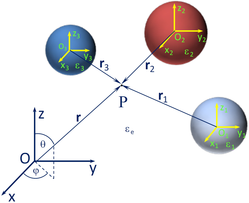
Figure 1: Schematics of the configuration of a system of scatterers consisting of three nanospheres embedded in a background medium. Also depicted are the global coordinate system with origin in $O$ and the local ones with origin in $O_{1}$, $O_{2}$, and $O_{3}$.

2.1 Geometrical configuration and material parameters

We seek to characterize the SHG from clusters of arbitrarily distributed spherical nanoparticles made of homogeneous and isotropic centrosymmetric materials. The cluster is illuminated by an incident monochromatic electromagnetic plane wave, $\{\mathbf{E}_{inc}^{\omega},\mathbf{H}_{inc}^{\omega}\}$, with angular fundamental frequency $\omega$. Also, we assume that all fields have a time-harmonic dependence, $e^{-i\omega t}$, which for the sake of simplicity is suppressed throughout the manuscript. We index the set of particles with the subscript $n$, which takes the values $n=1,2,\ldots,N$, with $N$ being the number of spherical scatterers.

The $n^{th}$ sphere, with radius $R_{n}$, is made of (possible dispersive) material described by the electric permittivity, $\epsilon_{n}$, and embedded in a lossless medium of permittivity $\epsilon_{e}$. The magnetic permeabilities of the particles and the background medium are the same and equal to the vacuum permeability, i.e. $\mu_{n}=\mu_{e}=\mu_{0}$. Furthermore, the nonlinear polarization, $\mathbf{P}_{n}^{\Omega}$, responsible for the SHG, is governed by the third-rank nonlinear susceptibility tensor, $\hat{\bm{\chi}}_{n}^{(2)}$. We label the origin of the global coordinate system of the cluster with $O$, and to each particle we associate a local coordinate system with origin $O_{n}$ located at the center of the corresponding sphere. The position of an arbitrary point, $P$, can be expressed in two ways: either with respect to the global coordinate system, via the spherical coordinates $(r,\theta,\phi)$, or in the local coordinate system associated to the $n^{th}$ sphere, using the spherical coordinates $(r_{n},\theta_{n},\phi_{n})$ – see Fig. 1.

2.2 Mathematical formulation of the T-matrix method

In principle, many numerical algorithms for solving Maxwell equations can be used to derive the transfer matrix relating the incident and scattered electromagnetic fields. If the particle under consideration is a homogeneous sphere, the surface integral equations expressed in terms of VSWFs, in conjunction with the EBC method, are an especially attractive choice. The decrease in the requirements of computer memory, as compared to the MoM-SIE, comes from the fact that the system matrix entries, which are related to certain integrals over the surface of the particle, can be evaluated analytically. The entries of the T-matrix computed in this way are equivalent to the coefficients used in the Mie series expansion of the electromagnetic field.

2.2.1 T-matrix formalism at the fundamental frequency

We divide the computational domain $V$ into an exterior subdomain $V_{e}$, occupied by the background medium, and interior subdomains $V_{n}$, $n=1,2,\ldots,N$, occupied by the spherical particles. The subdomains $V_{e}$ and $V_{n}$ are separated by oriented and closed boundaries of the nanoparticles, $S_{n}$, defined with the unit normal vector $\hat{\mathbf{n}}_{n}$ pointing towards the exterior domain $V_{e}$. The electromagnetic fields propagating at the FF satisfy the following Maxwell equations:

$$\nabla\times\mathbf{H}_{n}^{\omega}(\mathbf{r})=-i\omega\epsilon_{n}^{\omega}\mathbf{E}_{n}^{\omega}(\mathbf{r}),\quad\mathbf{r}\in V_{n},$$ (1a)

$$\nabla\times\mathbf{E}_{n}^{\omega}(\mathbf{r})=i\omega\mu_{0}\mathbf{H}_{n}^{\omega}(\mathbf{r}),\quad\mathbf{r}\in V_{n},$$ (1b)

and

$$\nabla\times\mathbf{H}_{s}^{\omega}(\mathbf{r})=-i\omega\epsilon_{e}\mathbf{E}_{s}^{\omega}(\mathbf{r}),\quad\mathbf{r}\in V_{e},$$ (2a)

$$\nabla\times\mathbf{E}_{s}^{\omega}(\mathbf{r})=i\omega\mu_{0}\mathbf{H}_{s}^{\omega}(\mathbf{r}),\quad\mathbf{r}\in V_{e},$$ (2b)

where $(\mathbf{E}_{n}^{\omega},\mathbf{H}_{n}^{\omega})$ are the fields inside the $n^{th}$ sphere and the scattered electromagnetic fields, $(\mathbf{E}_{s}^{\omega},\mathbf{H}_{s}^{\omega})$, are equal to the difference between the total exterior fields, $(\mathbf{E}_{e}^{\omega},\mathbf{H}_{e}^{\omega})$, and the incident fields $(\mathbf{E}_{inc}^{\omega},\mathbf{H}_{inc}^{\omega})$:

$$\mathbf{H}_{s}^{\omega}(\mathbf{r})=\mathbf{H}_{e}^{\omega}(\mathbf{r})-\mathbf{H}_{inc}^{\omega}(\mathbf{r}),\quad\mathbf{r}\in V_{e},$$ (3a)

$$\mathbf{E}_{s}^{\omega}(\mathbf{r})=\mathbf{E}_{e}^{\omega}(\mathbf{r})-\mathbf{E}_{inc}^{\omega}(\mathbf{r}),\quad\mathbf{r}\in V_{e}.$$ (3b)

Equations (1) and (2) are supplemented with the following boundary conditions expressing the continuity of the tangent components of the internal and external electric and magnetic fields, $\hat{\mathbf{n}}_{n}\times\mathbf{E}_{n}^{\omega}(\mathbf{r})|_{\mathbf{r}\in S_{n}}=\hat{\mathbf{n}}_{n}\times\mathbf{E}_{e}^{\omega}(\mathbf{r})|_{\mathbf{r}\in S_{n}}$ and $\hat{\mathbf{n}}_{n}\times\mathbf{H}_{n}^{\omega}(\mathbf{r})|_{\mathbf{r}\in S_{n}}=\hat{\mathbf{n}}_{n}\times\mathbf{H}_{e}^{\omega}(\mathbf{r})|_{\mathbf{r}\in S_{n}}$, defined on the surfaces $S_{n}$ and written as:

$$\hat{\mathbf{n}}_{n}\times[\mathbf{E}_{n}^{\omega}(\mathbf{r})-\mathbf{E}_{s}^{\omega}(\mathbf{r})]=\hat{\mathbf{n}}_{n}\times\mathbf{E}_{inc}^{\omega}(\mathbf{r}),\quad\mathbf{r}\in S_{n},$$ (4a)

$$\hat{\mathbf{n}}_{n}\times[\mathbf{H}_{n}^{\omega}(\mathbf{r})-\mathbf{H}_{s}^{\omega}(\mathbf{r})]=\hat{\mathbf{n}}_{n}\times\mathbf{H}_{inc}^{\omega}(\mathbf{r}),\quad\mathbf{r}\in S_{n}.$$ (4b)

In the framework of the T-matrix method, we expand the incident, scattered, and internal electric fields corresponding to each particle in terms of VSWFs, which represent a complete set of vector functions:

$$\mathbf{E}_{inc}^{\omega}(\mathbf{r})=E_{0}\sum\limits_{\nu\geq 1}\Big{[}q_{\nu}^{\omega}\mathbf{M}_{\nu}^{(1)}(k_{e}^{\omega}\mathbf{r})+p_{\nu}^{\omega}\mathbf{N}_{\nu}^{(1)}(k_{e}^{\omega}\mathbf{r})\Big{]},$$ (5a)

$$\mathbf{E}_{s}^{\omega}(\mathbf{r})=E_{0}\sum\limits_{n=1}^{N}\sum\limits_{\nu\geq 1}\Big{[}b_{n,\nu}^{\omega}\mathbf{M}_{\nu}^{(3)}(k_{e}^{\omega}\mathbf{r}_{n})+a_{n,\nu}^{\omega}\mathbf{N}_{\nu}^{(3)}(k_{e}^{\omega}\mathbf{r}_{n})\Big{]},$$ (5b)

$$\mathbf{E}_{n}^{\omega}(\mathbf{r})=E_{0}\sum\limits_{\nu\geq 1}\Big{[}c_{n,\nu}^{\omega}\mathbf{M}_{\nu}^{(1)}(k_{n}^{\omega}\mathbf{r}_{n})+d_{n,\nu}^{\omega}\mathbf{N}_{\nu}^{(1)}(k_{n}^{\omega}\mathbf{r}_{n})\Big{]},$$ (5c)

respectively, where $E_{0}$ is the amplitude of the incident wave, $k_{e}^{\omega}=\omega\sqrt{\epsilon_{e}\mu_{0}}$ is the wave number of the background medium, and $k_{n}^{\omega}=\omega\sqrt{\epsilon_{n}^{\omega}\mu_{0}}$ is the wave number of the medium in the particle $n$. The parameters $\{q_{\nu}^{\omega},p_{\nu}^{\omega}\}$ represent the expansion coefficients in the series expansion of the linearly polarized incident plane wave (see Appendix A for their definition), whereas $\{b_{n,\nu}^{\omega},a_{n,\nu}^{\omega}\}$ and $\{c_{n,\nu}^{\omega},d_{n,\nu}^{\omega}\}$ are the expansion coefficients of the scattered and internal fields, respectively, associated with the $n^{th}$ spherical particle. We label the spherical coordinates of the field-point $\mathbf{r}$, in the global coordinate system, with $(r,\theta,\phi)$. The same point is defined in the local coordinate system associated to the $n^{th}$ particle using the coordinates $(r_{n},\theta_{n},\phi_{n})\equiv\mathbf{r}_{n}$ (see Fig. 1). The multi-index $\nu=(l,m)$ combines the orbital and azimuthal indices $l$ and $m$, respectively, so that the summation over this index is denoted as $\sum_{\nu\geq 1}\equiv\sum_{l\geq 1}\sum_{m=-l}^{l}$.

The choice of VSWFs $\mathbf{M}_{\nu}^{(J)}$ and $\mathbf{N}_{\nu}^{(J)}$, $J=1,3$, in equations (5) is guided by the following considerations: the incident and the internal fields are expanded in series of regular VSWFs $\mathbf{M}_{\nu}^{(1)}$ and $\mathbf{N}_{\nu}^{(1)}$, which are finite at origin, whereas the scattered fields are expanded in series of outgoing VSWFs, $\mathbf{M}_{\nu}^{(3)}$ and $\mathbf{N}_{\nu}^{(3)}$, which satisfy the radiation boundary condition at infinity. The expansion of the magnetic fields in VSWFs is derived from equations (5) by using expressions (1b) and (2b).

In the case of a single particle, the relation between the incident and the scattering coefficients associated with the VSWF-expansion of the FF fields can be written as follows [36]:

$$\mathbf{f}_{n}^{\omega}=\mathbf{T}_{n}^{\omega}\mathbf{g}_{n}^{\omega},$$ (6)

where $\mathbf{T}_{n}^{\omega}$ is the transfer matrix of the $n^{th}$ particle and has size of $2N_{max}\times 2N_{max}$, and $\mathbf{f}_{n}^{\omega}=[b_{n,\nu}^{\omega},a_{n,\nu}^{\omega}]^{\mathrm{T}}$ and $\mathbf{g}_{n}^{\omega}=[q_{n,\nu}^{\omega},p_{n,\nu}^{\omega}]^{\mathrm{T}}$, $\nu=1\ldots N_{max}$, are vectors containing the expansion coefficients of the scattered and incident fields expanded in the local coordinates, respectively. Moreover, $N_{max}=l_{max}^{2}+2l_{max}$ is the number of Fourier coefficients in the series expansion, with $l_{max}$ being the cut-off value for the orbital index, $l$.

For the particular case of a spherical particle, $\mathbf{T}_{n}^{\omega}$ is a diagonal matrix with entries that can be calculated by imposing the boundary conditions (4) on the VSWF-field expansions. These diagonal elements are the well-known transverse electric and transverse magnetic Mie coefficients [49]. If the particle is of arbitrary shape, the matrix $\mathbf{T}_{n}^{\omega}$ is usually full.

The transfer matrix $\mathbf{T}_{n}^{\omega}$ pertaining to a scatterer of arbitrary shape can be calculated using a matrix $\mathbf{Q}_{n}^{\omega(1,3)}$, which relates the incident and internal field coefficients:

$$\mathbf{h}_{n}^{\omega}=-[\mathbf{Q}_{n}^{\omega(1,3)}]^{-1}\mathbf{g}_{n}^{\omega},$$ (7)

where the vector $\mathbf{h}_{n}^{\omega}=[c_{n,\nu}^{\omega},d_{n,\nu}^{\omega}]^{\mathrm{T}}$ contains the internal field expansion coefficients. The relation (7) is a direct consequence of the equivalence principle applied to the region inside the particle. The notation (1,3) indicates that the products of VSWFs in the integrals taken over the surface of the particle, and which define the entries of the matrix $\mathbf{Q}_{n}^{\omega(1,3)}$, contain a regular and a radiating function (for the definition of these integrals, see e.g. Refs. [50, 51]). In the case of axisymmetric particles, the 2D surface integrals can be reduced to 1D line integrals, whereas in the particular case of a sphere, these integrations can be evaluated analytically exploiting the orthogonality of VSWFs on a sphere. This reduced computational complexity is perhaps the reason why the vast majority of the studies based on TMM consider rotationally symmetric scatterers. It can be seen then that the transfer matrix $\mathbf{T}_{n}^{\omega}$ for an arbitrarily shaped scatterer can be calculated using the following relation:

$$\mathbf{T}_{n}^{\omega}=-\mathbf{Q}_{n}^{\omega(1,1)}[\mathbf{Q}_{n}^{\omega(1,3)}]^{-1},$$ (8)

where the integrals defining the matrix elements of $\mathbf{Q}_{n}^{\omega(1,1)}$ contain only regular VSWFs.

It is well known that the standard TMM is less accurate when applied to situations in which the near-field is highly inhomogeneous. This usually occurs when one deals with scatterers with sharp edges and corners or objects with large permittivity. In order to circumvent this pitfall, a TMM that exploits the discrete VSWFs has been introduced [50]. However, if one needs to determine very accurately the optical near-field in the vicinity of sharp tips, as required for example in sensing applications, MoM-SIE is the method of choice [52].

In the case of a multiparticle system illuminated by a plane wave, the coupling between the scatterers (multiple scattering) has to be taken into account. To this end, the total electric field exciting the $n^{th}$ particle can be expressed as the sum of the incident field and the field scattered from all the other particles:

$$\mathbf{E}_{n,ex}^{\omega}(\mathbf{r})= E_{0}\left[\mathbf{M}_{\nu}^{(1)}(k_{e}^{\omega}\mathbf{r}),\mathbf{N}_{\nu}^{(1)}(k_{e}^{\omega}\mathbf{r})\right]\mathbf{g}^{\omega}$$ (9)

$$+E_{0}\sum\limits_{\begin{subarray}{c}k=1\\ k\neq n\end{subarray}}^{N}\left[\mathbf{M}_{\nu}^{(3)}(k_{e}^{\omega}\mathbf{r}_{k}),\mathbf{N}_{\nu}^{(3)}(k_{e}^{\omega}\mathbf{r}_{k})\right]\mathbf{f}_{k}^{\omega},\quad n=1,\ldots,N.$$

This field is expanded around the origin of the $n^{th}$ sphere as:

$$\mathbf{E}_{n,ex}^{\omega} (\mathbf{r}_{n})=E_{0}\left[\mathbf{M}_{\nu}^{(1)}(k_{e}^{\omega}\mathbf{r}_{n}),\mathbf{N}_{\nu}^{(1)}(k_{e}^{\omega}\mathbf{r}_{n})\right]\bm{\beta}_{n,0}^{\omega}\mathbf{g}^{\omega}$$ (10)

$$+E_{0}\sum\limits_{\begin{subarray}{c}k=1\\ k\neq n\end{subarray}}^{N}\left[\mathbf{M}_{\nu}^{(1)}(k_{e}^{\omega}\mathbf{r}_{n}),\mathbf{N}_{\nu}^{(1)}(k_{e}^{\omega}\mathbf{r}_{n})\right]\bm{\alpha}_{n,k}^{\omega}\mathbf{f}_{k}^{\omega},\quad n=1,\ldots,N.$$

In this equation, the matrices $\bm{\alpha}_{n,k}^{\omega}$ and $\bm{\beta}_{n,0}^{\omega}$, $n,k=1,\ldots,N$, represent normalized irregular and regular translation-addition matrices, respectively, evaluated at angular frequency $\omega$ [53, 54, 55]. The irregular translation-addition matrix $\bm{\alpha}_{n,k}^{\omega}$ transforms the radiating (outgoing) spherical harmonics $(J=3)$ expanded around the origin $O_{k}$, to the regular spherical harmonics $(J=1)$ expanded around the origin $O_{n}$. The regular translation-addition matrix $\bm{\beta}_{n,k}^{\omega}$ transforms the (regular or outgoing) VSWFs expressed in a coordinate system with origin in $O_{k}$ to the same (regular or outgoing) VSWFs expressed in a coordinate system with origin in $O_{n}$. As illustrated by (10), for each scatterer $n$, one uses the regular translation matrix $\bm{\beta}_{n,0}^{\omega}$ to translate the incident field expansion around the origin of the global coordinate system, $O$, to the expansion around the origin of the local coordinate system, $O_{n}$, associated to the $n^{th}$ spherical scatterer, i.e. $\mathbf{g}_{n}^{\omega}=\bm{\beta}_{n,0}^{\omega}\mathbf{g}^{\omega}$.

The total field that excites the $n^{th}$ particle, $\mathbf{E}_{n,ex}^{\omega}(\mathbf{r}_{n})$, can itself be expanded into Fourier series of VSWFs, $\mathbf{M}_{\nu}^{(1)}(k_{e}^{\omega}\mathbf{r}_{n})$ and $\mathbf{N}_{\nu}^{(1)}(k_{e}^{\omega}\mathbf{r}_{n})$, with the corresponding Fourier coefficients being $\mathbf{e}_{n}^{\omega}$. Then, as (10) indicates, these expansion coefficients can be expressed as:

$$\mathbf{e}_{n}^{\omega}=\bm{\beta}_{n,0}^{\omega}\mathbf{g}^{\omega}+\sum\limits_{\begin{subarray}{c}k=1\\ k\neq n\end{subarray}}^{N}\bm{\alpha}_{n,k}^{\omega}\mathbf{f}_{k}^{\omega},\quad n=1,\ldots,N.$$ (11)

Multiplying to the left this equation with $\mathbf{T}_{n}^{\omega}$ and using the definition of the transfer matrix for a single scatterer, one can recast (11) in terms of the expansion coefficients of the scattering field as follows:

$$\mathbf{f}_{n}^{\omega}=\mathbf{T}_{n}^{\omega}\bm{\beta}_{n,0}^{\omega}\mathbf{g}^{\omega}+\sum\limits_{\begin{subarray}{c}k=1\\ k\neq n\end{subarray}}^{N}\mathbf{T}_{n}^{\omega}\bm{\alpha}_{n,k}^{\omega}\mathbf{f}_{k}^{\omega},\quad n=1,\ldots,N.$$ (12)

These equations can be collected together and expressed as a single matrix equation in the following form [36]:

$$\begin{bmatrix}\textbf{I}&-\textbf{T}_{1}^{\omega}\bm{\alpha}_{1,2}^{\omega}&\cdots&-\textbf{T}_{1}^{\omega}\bm{\alpha}_{1,N}^{\omega}\\ -\textbf{T}_{2}^{\omega}\bm{\alpha}_{2,1}^{\omega}&\textbf{I}&\cdots&-\textbf{T}_{2}^{\omega}\bm{\alpha}_{2,N}^{\omega}\\ \vdots&\vdots&\ddots&\vdots\\ -\textbf{T}_{N}^{\omega}\bm{\alpha}_{N,1}^{\omega}&-\textbf{T}_{N}^{\omega}\bm{\alpha}_{N,2}^{\omega}&\cdots&\textbf{I}\end{bmatrix}\begin{bmatrix}\textbf{f}_{1}^{\omega}\\ \textbf{f}_{2}^{\omega}\\ \vdots\\ \textbf{f}_{N}^{\omega}\end{bmatrix}=\begin{bmatrix}\textbf{T}_{1}^{\omega}\bm{\beta}_{1,0}^{\omega}\textbf{g}^{\omega}\\ \textbf{T}_{2}^{\omega}\bm{\beta}_{2,0}^{\omega}\textbf{g}^{\omega}\\ \vdots\\ \textbf{T}_{N}^{\omega}\bm{\beta}_{N,0}^{\omega}\textbf{g}^{\omega}\\ \end{bmatrix},$$ (13)

or in a more condensed form,

$$\mathbf{S}^{\omega}\mathbf{F}^{\omega}=\mathbf{G}^{\omega}.$$ (14)

The matrix $\mathbf{S}^{\omega}$ is the scattering matrix of the cluster at the FF, $\mathbf{F}^{\omega}=\{\mathbf{f}_{n}^{\omega}\}$, $n=1\ldots N$, is the vector containing the unknowns, namely the expansion coefficients of the scattered field, and $\mathbf{G}^{\omega}=\{\textbf{T}_{n}^{\omega}\bm{\beta}_{n,0}^{\omega}\textbf{g}^{\omega}\}$, $n=1\ldots N$, is the vector containing the expansion coefficients associated with the incident field. The unknown scattering field coefficients corresponding to each particle are obtained by simply solving the linear system (13).

The scattering cross-section (SCS) and absorption cross-section (ACS), calculated at frequency $\omega$, are then easily obtained from these scattering field coefficients using relatively simple relations [55, 56]:

$$\sigma_{sca}^{\omega}=\frac{1}{(k_{e}^{\omega})^{2}}\sum\limits_{n,k=1}^{N}\mathfrak{Re}\{\textbf{f}_{n}^{\omega*}\bm{\beta}_{n,k}^{\omega}\textbf{f}_{k}^{\omega}\},$$ (15)

$$\sigma_{abs}^{\omega}=\frac{1}{(k_{e}^{\omega})^{2}}\sum\limits_{n=1}^{N}\textbf{f}_{n}^{\omega*}\bm{\Gamma}_{n}^{\omega}\textbf{f}_{n}^{\omega},$$ (16)

where the symbol “$*$” denotes complex conjugation, $\mathfrak{Re}\{z\}$ is the real part of the complex number $z$, and $\bm{\Gamma}_{n}^{\omega}$ is a matrix that transforms the scattering coefficients to the internal field expansion coefficients. It can be easily calculated from the field boundary conditions (see, e.g. Ref. [55, 56]).

2.2.2 T-matrix formalism at the second-harmonic frequency

In the second step of our numerical method, we use the fields at the FF, computed at the linear step just described, and subsequently compute the sources at the SH frequency. Here, we focus on SHG analysis from centrosymmetric materials widely used in nonlinear optics, including noble metals (Au, Ag) and dielectrics (Si, $\mathrm{SiO_{2}}$) in which the crystal lattice is invariant upon inversion symmetry transformations. Due to the centrosymmetry of the material, the (local) bulk second-order susceptibility tensor $\hat{\bm{\chi}}^{(2)}$ identically vanishes inside the particle. However, the inversion symmetry property is locally broken at the surface of the centrosymmetric material [4, 5, 6, 2, 3], and the corresponding surface SHG is described by a third-rank nonlinear susceptibility tensor, $\hat{\boldsymbol{\chi}}_{s}^{(2)}$. In the bulk of the centrosymmetric material, the (nonlocal) sources of SH consist of nonlinear electric quadrupoles and nonlinear magnetic dipoles, the corresponding SHG being described by a fourth-rank nonlinear susceptibility tensor $\hat{\boldsymbol{\chi}}_{b}^{(2)}$.

Putting these ideas together, the nonlinear polarization, $\mathbf{P}^{\Omega}(\mathbf{r})$, that generates the SH field can be represented as the sum of the local surface and nonlocal bulk contributions as:

$$\mathbf{P}^{\Omega}(\mathbf{r})= \mathbf{P}_{s}^{\Omega}(\mathbf{r})+\mathbf{P}_{b}^{\Omega}(\mathbf{r})=\epsilon_{0}\hat{\boldsymbol{\chi}}_{s}^{(2)}:\mathbf{E}^{\omega}(\mathbf{r})\mathbf{E}^{\omega}(\mathbf{r})\delta(\mathbf{r}-\mathbf{r}_{s})$$

$$+\epsilon_{0}\hat{\boldsymbol{\chi}}_{b}^{(2)}\vdots\mathbf{E}^{\omega}(\mathbf{r})[\nabla\mathbf{E}^{\omega}(\mathbf{r})]\left.\right|_{\mathbf{r}\in V},$$ (17)

where $S=\bigcup_{n=1}^{N}S_{n}$ ($V=\bigcup_{n=1}^{N}V_{n}$) is the total surface (volume) of the particles and $\mathbf{r}_{s}\in S$ defines the surface $S$. In equation (2.2.2), the factors $\mathbf{E}^{\omega}(\mathbf{r})\mathbf{E}^{\omega}(\mathbf{r})$ and $\mathbf{E}^{\omega}(\mathbf{r})[\nabla\mathbf{E}^{\omega}(\mathbf{r})]$ represent second- and third-rank tensors, respectively, so that the nonlinear polarization in (2.2.2) can be written componentwise as:

$$P_{i}^{\Omega}=\epsilon_{0}\hat{\chi}_{ijk}^{(2)}E_{j}^{\omega}E_{k}^{\omega}\delta(\mathbf{r}-\mathbf{r}_{s})+\epsilon_{0}\hat{\chi}_{ijkl}^{(2)}E_{j}^{\omega}\nabla_{k}E_{l}^{\omega}\left.\right|_{\mathbf{r}\in V},$$ (18)

where Einstein summation convention is assumed. Note that the electric fields in the surface term of (2.2.2) should be evaluated just beneath the particle boundary.

The surface nonlinear susceptibility tensor $\hat{\bm{\chi}}_{s}^{(2)}$ has 27 components, but for homogeneous and isotropic surfaces only three of them are independent. These components are $\chi_{s,\perp\perp\perp}^{(2)}$, $\chi_{s,\perp\parallel\parallel}^{(2)}$, and $\chi_{s,\parallel\perp\parallel}^{(2)}=\chi_{s,\parallel\parallel\perp}^{(2)}$ [3], defined with respect to the local orthonormal coordinate system located at each point on the surface, and the subscripts $\bot$ and $\parallel$ refer to the orientations perpendicular and parallel to the boundary, respectively. The surface nonlinear polarization sheet, $\bm{\mathcal{P}}_{s}^{\Omega}$, defined by the relation $\mathbf{P}_{s}^{\Omega}(\mathbf{r})\equiv\bm{\mathcal{P}}_{s}^{\Omega}(\mathbf{r})\delta(\mathbf{r}-\mathbf{r}_{s})$, can be expressed in spherical coordinates associated to the sphere as:

$$\mathcal{P}_{s,r}^{\Omega}=\epsilon_{0}\left[\hat{\chi}_{s,\perp\perp\perp}^{(2)}E_{r}^{\omega}E_{r}^{\omega}+\hat{\chi}_{s,\perp\parallel\parallel}^{(2)}(E_{\theta}^{\omega}E_{\theta}^{\omega}+E_{\phi}^{\omega}E_{\phi}^{\omega})\right],$$ (19a)

$$\mathcal{P}_{s,\theta}^{\Omega}=2\epsilon_{0}\hat{\chi}_{s,\parallel\perp\parallel}^{(2)}E_{r}^{\omega}E_{\theta}^{\omega},$$ (19b)

$$\mathcal{P}_{s,\phi}^{\Omega}=2\epsilon_{0}\hat{\chi}_{s,\parallel\perp\parallel}^{(2)}E_{r}^{\omega}E_{\phi}^{\omega}.$$ (19c)

The bulk nonlinear polarization contribution $\mathbf{P}_{b}^{\Omega}$ can be cast in the following form [12]:

$$\mathbf{P}_{b}^{\Omega}=\epsilon_{0}\beta\mathbf{E}^{\omega}\nabla\cdot\mathbf{E}^{\omega}+\epsilon_{0}\gamma\nabla(\mathbf{E}^{\omega}\cdot\mathbf{E}^{\omega})+\epsilon_{0}\delta^{\prime}(\mathbf{E}^{\omega}\cdot\nabla)\mathbf{E}^{\omega},$$ (20)

where $\beta$, $\gamma$ and $\delta^{\prime}$ are material parameters. The first term in (20) vanishes in homogeneous materials since there is no net charge density present in the bulk of the material, whereas the last term can be neglected as well, as most theoretical models predict [57].

The electromagnetic fields at the SH frequency, $\Omega$, are generated by the nonlinear polarization sources, $\mathbf{P}_{n}^{\Omega}$, $n=1,2,\ldots,N$, associated to each sphere. These nonlinear fields satisfy the following inhomogeneous system of equations:

$$\nabla\times\mathbf{H}_{n}^{\Omega}(\mathbf{r})+i\Omega\epsilon_{n}^{\Omega}\mathbf{E}_{n}^{\Omega}(\mathbf{r})=-i\Omega\mathbf{P}_{b,n}^{\Omega}(\mathbf{r}),\quad\mathbf{r}\in V_{n},$$ (21a)

$$\nabla\times\mathbf{E}_{n}^{\Omega}(\mathbf{r})-i\Omega\mu_{0}\mathbf{H}_{n}^{\Omega}(\mathbf{r})=0.\quad\mathbf{r}\in V_{n},$$ (21b)

Moreover, the external nonlinear fields satisfy the following homogeneous equations:

$$\nabla\times\mathbf{H}_{e}^{\Omega}(\mathbf{r})+i\Omega\epsilon_{e}\mathbf{E}_{e}^{\Omega}(\mathbf{r})=0,\quad\mathbf{r}\in V_{e},$$ (22a)

$$\nabla\times\mathbf{E}_{e}^{\Omega}(\mathbf{r})-i\Omega\mu_{0}\mathbf{H}_{e}^{\Omega}(\mathbf{r})=0,\quad\mathbf{r}\in V_{e}.$$ (22b)

In addition to (21) and (22), the components of the internal and external nonlinear fields tangent to the surface $S_{n}$ of the $n^{th}$ sphere, $n=1,2,\ldots,N$, are subject to the nonlinear boundary conditions (see Appendix B) [58]:

$$\hat{\mathbf{n}}_{n}\times[\mathbf{E}_{e}^{\Omega}(\mathbf{r})-\mathbf{E}_{n}^{\Omega}(\mathbf{r})]=-\bm{\mathcal{M}}_{n}^{\Omega},\quad\mathbf{r}\in S_{n},$$ (23a)

$$\hat{\mathbf{n}}_{n}\times[\mathbf{H}_{e}^{\Omega}(\mathbf{r})-\mathbf{H}_{n}^{\Omega}(\mathbf{r})]=\bm{\mathcal{J}}_{n}^{\Omega},\quad\mathbf{r}\in S_{n}.$$ (23b)

In these equations, the magnetic and electric surface currents, $\bm{\mathcal{M}}_{n}^{\Omega}(\theta_{n},\phi_{n})$ and $\bm{\mathcal{J}}_{n}^{\Omega}(\theta_{n},\phi_{n})$, respectively, are determined by the normal and tangent contributions of the surface nonlinear polarization sheet, $\bm{\mathcal{P}}_{s}^{\Omega}(\theta_{n},\phi_{n})$, with all these surface vector functions depending only on the coordinates $(\theta_{n},\phi_{n})$ describing the tangent plane at $\mathbf{r}_{n}$:

$$\bm{\mathcal{J}}_{n}^{\Omega}(\mathbf{r})=i\Omega\hat{\mathbf{n}}_{n}\times\left[\hat{\mathbf{n}}_{n}\times\bm{\mathcal{P}}_{s,n}^{\Omega}(\mathbf{r})\right],\quad\mathbf{r}\in S_{n},$$ (24a)

$$\bm{\mathcal{M}}_{n}^{\Omega}(\mathbf{r})=\frac{1}{\epsilon_{0}}\hat{\mathbf{n}}_{n}\times\nabla_{S}\left[\hat{\mathbf{n}}_{n}\cdot\bm{\mathcal{P}}_{s,n}^{\Omega}(\mathbf{r})\right],\quad\mathbf{r}\in S_{n},$$ (24b)

where $\nabla_{S}$ acts in the tangent plane at $\mathbf{r}\in S_{n}$.

In order to solve the systems of partial differential equations, (21) and (22), together with the boundary conditions (23), one has to find the general solution of both homogeneous systems and the particular solution satisfying the inhomogeneous system of equations (21).

The two homogeneous systems of equations describing the SH process can be written as:

$$\nabla\times\bar{\mathbf{H}}_{n}^{\Omega}(\mathbf{r})+i\Omega\epsilon_{n}^{\Omega}\bar{\mathbf{E}}_{n}^{\Omega}(\mathbf{r})=0,\quad\mathbf{r}\in V_{n},$$ (25a)

$$\nabla\times\bar{\mathbf{E}}_{n}^{\Omega}(\mathbf{r})-i\Omega\mu_{0}\bar{\mathbf{H}}_{n}^{\Omega}(\mathbf{r})=0,\quad\mathbf{r}\in V_{n},$$ (25b)

and

$$\nabla\times\bar{\mathbf{H}}_{e}^{\Omega}(\mathbf{r})+\Omega i\epsilon_{e}\bar{\mathbf{E}}_{e}^{\Omega}(\mathbf{r})=0,\quad\mathbf{r}\in V_{e},$$ (26a)

$$\nabla\times\bar{\mathbf{E}}_{e}^{\Omega}(\mathbf{r})-\Omega i\mu_{0}\bar{\mathbf{H}}_{e}^{\Omega}(\mathbf{r})=0,\quad\mathbf{r}\in V_{e},$$ (26b)

where $\left\{\bar{\mathbf{E}}_{n}^{\Omega},\bar{\mathbf{H}}_{n}^{\Omega}\right\}$ and $\left\{\bar{\mathbf{E}}_{e}^{\Omega},\bar{\mathbf{H}}_{e}^{\Omega}\right\}$, are the SH electromagnetic field solutions satisfying the homogeneous systems of equations (25) and (26), valid inside the $n^{th}$ particle and in the exterior domain, respectively. The external homogeneous field solution $\left\{\bar{\mathbf{E}}_{e}^{\Omega},\bar{\mathbf{H}}_{e}^{\Omega}\right\}$ must obey the Silver-Müller radiation condition. The general solution of the two systems (21) and (22) is then:

$$\mathbf{H}_{n}^{\Omega}(\mathbf{r})=\bar{\mathbf{H}}_{n}^{\Omega}(\mathbf{r})+\mathbf{H}_{n}^{\Omega,p}(\mathbf{r}),\quad\mathbf{r}\in V_{n},$$ (27a)

$$\mathbf{E}_{n}^{\Omega}(\mathbf{r})=\bar{\mathbf{E}}_{n}^{\Omega}(\mathbf{r})+\mathbf{E}_{n}^{\Omega,p}(\mathbf{r}),\quad\mathbf{r}\in V_{n},$$ (27b)

and

$$\mathbf{H}_{e}^{\Omega}(\mathbf{r})=\bar{\mathbf{H}}_{e}^{\Omega}(\mathbf{r}),\quad\mathbf{r}\in V_{e},$$ (28a)

$$\mathbf{E}_{e}^{\Omega}(\mathbf{r})=\bar{\mathbf{E}}_{e}^{\Omega}(\mathbf{r}),\quad\mathbf{r}\in V_{e},$$ (28b)

where $\left(\mathbf{E}_{n}^{\Omega,p},\mathbf{H}_{n}^{\Omega,p}\right)$ is the particular solution of the inhomogeneous system (21). Considering that $\nabla\times\nabla F(\mathbf{r})=0$ for any scalar function $F(\mathbf{r})$, it can be seen that a particular solution of the inhomogeneous system (21) is given by:

$$\mathbf{H}_{n}^{\Omega,p}(\mathbf{r})=0,\quad\mathbf{r}\in V_{n}$$ (29a)

$$\mathbf{E}_{n}^{\Omega,p}(\mathbf{r})=-\frac{1}{\epsilon_{n}^{\Omega}}\mathbf{P}_{b,n}^{\Omega}(\mathbf{r})=-\frac{\epsilon_{0}\gamma}{\epsilon_{n}^{\Omega}}\nabla\left[\mathbf{E}_{n}^{\omega}(\mathbf{r})\cdot\mathbf{E}_{n}^{\omega}(\mathbf{r})\right],\quad\mathbf{r}\in V_{n}.$$ (29b)

Exploiting the nonlinear boundary conditions (23) and decomposition of the nonlinear SH fields to homogeneous and particular components, as per (27) and (28), we can express the boundary conditions for the SH homogeneous field solutions as:

$$\hat{\mathbf{n}}_{n}\times[\bar{\mathbf{E}}_{e}^{\Omega}(\mathbf{r})-\bar{\mathbf{E}}_{n}^{\Omega}(\mathbf{r})]=-\bm{\mathcal{M}}_{n}^{\Omega}(\mathbf{r})+\hat{\mathbf{n}}_{n}\times\mathbf{E}_{n}^{\Omega,p}(\mathbf{r}),\quad\mathbf{r}\in S_{n},$$ (30a)

$$\hat{\mathbf{n}}_{n}\times[\bar{\mathbf{H}}_{e}^{\Omega}(\mathbf{r})-\bar{\mathbf{H}}_{n}^{\Omega}(\mathbf{r})]=\bm{\mathcal{J}}_{n}^{\Omega}(\mathbf{r}),\quad\mathbf{r}\in S_{n}.$$ (30b)

We stress that the nonlinear surface polarization source $\mathbf{P}_{s,n}^{\Omega}$ does not explicitly enter in the equations describing the SH process, namely expressions (21) and (22), but rather it contributes to the nonlinear fields at the SH via the nonlinear boundary conditions imposed at the surface of the particles, as per (23).

It can be easily seen that the homogeneous systems of equations (25) and (26) at the SH, together with the corresponding boundary conditions (30), are similar to the system of equations (1) and (2) at the FF and the accompanying boundary conditions (4) for the linear fields. Therefore, in similar fashion to the series expansion in terms of VSWFs of the electromagnetic fields at the FF introduced in the preceding subsection, we proceed by expanding the SH external and internal electric fields $\bar{\mathbf{E}}_{e}^{\Omega}$ and $\bar{\mathbf{E}}_{n}^{\Omega}$, respectively, as [19]:

$$\bar{\mathbf{E}}_{e}^{\Omega}(\mathbf{r})=E_{0}^{2}\sum\limits_{n=1}^{N}\sum\limits_{\nu\geq 1}\left[b_{n,\nu}^{\Omega}\mathbf{M}_{\nu}^{(3)}(k_{e}^{\Omega}\mathbf{r}_{n})+a_{n,\nu}^{\Omega}\mathbf{N}_{\nu}^{(3)}(k_{e}^{\Omega}\mathbf{r}_{n})\right],$$ (31a)

$$\bar{\mathbf{E}}_{n}^{\Omega}(\mathbf{r})=E_{0}^{2}\sum\limits_{\nu\geq 1}\left[c_{n,\nu}^{\Omega}\mathbf{M}_{\nu}^{(1)}(k_{n}^{\Omega}\mathbf{r}_{n})+d_{n,\nu}^{\Omega}\mathbf{N}_{\nu}^{(1)}(k_{n}^{\Omega}\mathbf{r}_{n})\right],$$ (31b)

where the $\sim$$E_{0}^{2}$ dependence of the nonlinear fields on the amplitude of the (linear) excitation field has been explicitly introduced and $k_{e}^{\Omega}$ and $k_{n}^{\Omega}$ are the wave numbers in the background medium and interior of the $n^{th}$ sphere, respectively, calculated at the frequency $\Omega$.

Similarly to the fundamental frequency VSWF-expansions of the fields introduced in (5b) and (5c), the unknown coefficients $\{b_{n,\nu}^{\Omega},a_{n,\nu}^{\Omega}\}$ and $\{c_{n,\nu}^{\Omega},d_{n,\nu}^{\Omega}\}$ are used in the series expansion of the SH fields in terms of VSWFs. Moreover, in conjunction with (31), the series expansions in terms of VSWFs of the magnetic fields $\bar{\mathbf{H}}_{n}^{\Omega}$ and $\bar{\mathbf{H}}_{e}^{\Omega}$ can be easily obtained from (25b) and (26b), respectively.

A key step in the calculation of the unknown expansion coefficients $\{b_{n,\nu}^{\Omega},a_{n,\nu}^{\Omega}\}$ and $\{c_{n,\nu}^{\Omega},d_{n,\nu}^{\Omega}\}$ of the SH fields is the expansion of the vector functions in the r.h.s. of the nonlinear homogeneous boundary conditions (30), related to the $n^{th}$ particle, in series of vector spherical harmonic (VSH) functions (for the definition of these functions and their relation to VSWFs $\mathbf{M}_{\nu}^{(J)}$ and $\mathbf{N}_{\nu}^{(J)}$ see Appendix A). The three VSH functions are mutually orthogonal: the function $\mathbf{Y}_{\nu}$ points in the radial direction, whereas the the other two functions, $\mathbf{X}_{\nu}$ and $\mathbf{Z}_{\nu}$, lie in the plane tangent to the sphere. Therefore, the (tangential) SH homogeneous boundary conditions (30) can be expanded in series of (transverse) VSH functions $\mathbf{X}_{\nu}(\theta_{n},\phi_{n})$ and $\mathbf{Z}_{\nu}(\theta_{n},\phi_{n})$ [19]:

$$\bm{\mathcal{J}}_{n}^{\Omega}=\hat{\mathbf{n}}_{n}\times\left[\frac{iE_{0}^{2}}{Z_{e}}\sum\limits_{\nu\geq 1}\left(u_{n,\nu}^{{}^{\prime}\Omega}\mathbf{X}_{\nu}+v_{n,\nu}^{{}^{\prime}\Omega}\mathbf{Z}_{\nu}\right)\right],$$ (32a)

$$-\bm{\mathcal{M}}_{n}^{\Omega}+\hat{\mathbf{n}}_{n}\times\mathbf{E}_{n}^{\Omega,p}\big{|}_{S_{n}}=\hat{\mathbf{n}}_{n}\times\left[E_{0}^{2}\sum\limits_{\nu\geq 1}\left(u_{n,\nu}^{{}^{\prime\prime}\Omega}\mathbf{Z}_{\nu}+v_{n,\nu}^{{}^{\prime\prime}\Omega}\mathbf{X}_{\nu}\right)\right],$$ (32b)

where $Z_{e}=\sqrt{\nicefrac{{\mu_{0}}}{{\epsilon_{e}}}}$ is the impedance of the background medium and $\{u_{n,\nu}^{{}^{\prime}\Omega},v_{n,\nu}^{{}^{\prime}\Omega}\}$ and $\{u_{n,\nu}^{{}^{\prime\prime}\Omega},v_{n,\nu}^{{}^{\prime\prime}\Omega}\}$ are Fourier coefficients, which can be determined by calculating certain integrals over the surface of the unit sphere, utilizing the orthogonality properties of spherical harmonics [17, 34]. The surface integrations can be done analytically and the results are expressed in terms of Clebsch-Gordan series, given in [19].

The SH T-matrix corresponding to the $n^{th}$ sphere, with $n=1,\ldots,N$, which relates the external field coefficients, $\{b_{n,\nu}^{\Omega},a_{n,\nu}^{\Omega}\}$, to the coefficients used in the expansion of the SH sources, $\{u_{n,\nu}^{{}^{\prime}\Omega},v_{n,\nu}^{{}^{\prime}\Omega}\}$ and $\{u_{n,\nu}^{{}^{\prime\prime}\Omega},v_{n,\nu}^{{}^{\prime\prime}\Omega}\}$, can be written as:

$$\mathbf{f}_{n}^{\Omega}=\mathbf{T}_{n}^{\Omega}\mathbf{g}_{n}^{\Omega}.$$ (33)

Similarly to the FF T-matrix (6), the SH T-matrix of a single spherical particle, $\mathbf{T}_{n}^{\Omega}$, is a diagonal matrix with the entries computed by imposing the nonlinear homogeneous boundary conditions (30) to the SH field expansions (31). The vector $\mathbf{g}_{n}^{\Omega}$ contains the SH source-field expansion coefficients, $\mathbf{g}_{n}^{\Omega}=[v_{n,\nu}^{{}^{\prime}\Omega},u_{n,\nu}^{{}^{\prime}\Omega},v_{n,\nu}^{{}^{\prime\prime}\Omega},u_{n,\nu}^{{}^{\prime\prime}\Omega}]^{\mathrm{T}}$, and is determined by the FF field, whereas the vector $\mathbf{f}_{n}^{\Omega}$ holds the coefficients of the series expansion in VSWFs of the external SH field, $\mathbf{f}_{n}^{\Omega}=[b_{n,\nu}^{{}^{\prime}\Omega},a_{n,\nu}^{{}^{\prime}\Omega},b_{n,\nu}^{{}^{\prime\prime}\Omega},a_{n,\nu}^{{}^{\prime\prime}\Omega}]^{\mathrm{T}}$, where $b_{n,\nu}^{\Omega}=b_{n,\nu}^{{}^{\prime}\Omega}+b_{n,\nu}^{{}^{\prime\prime}\Omega}$ and $a_{n,\nu}^{\Omega}=a_{n,\nu}^{{}^{\prime}\Omega}+a_{n,\nu}^{{}^{\prime\prime}\Omega}$.

The extension to a multiparticle system is straightforward and analogous to the approach used in the case of the derivation of the FF multiparticle scattering matrix (13). The total SH electric field exciting the $n^{th}$ sphere is equal to the sum of the fields radiated by all the other spheres, and is given by:

$$\mathbf{E}_{n,ex}^{\Omega}(\mathbf{r})=E^{2}_{0}\sum\limits_{\begin{subarray}{c}k=1\\ k\neq n\end{subarray}}^{N}\left[\mathbf{M}_{\nu}^{(3)}(k_{e}^{\Omega}\mathbf{r}_{k}),\mathbf{N}_{\nu}^{(3)}(k_{e}^{\Omega}\mathbf{r}_{k})\right]\mathbf{f}_{k}^{\Omega},$$ (34)

$$\quad n=1,\ldots,N.$$

This field can be expanded in the local coordinates associated to the $n^{th}$ sphere employing the translation-addition matrices $\bm{\alpha}_{n,k}^{\Omega}$, evaluated at the SH frequency $\Omega$, as:

$$\mathbf{E}_{n,ex}^{\Omega}(\mathbf{r}_{n})=E^{2}_{0}\sum\limits_{\begin{subarray}{c}k=1\\ k\neq n\end{subarray}}^{N}\left[\mathbf{M}_{\nu}^{(1)}(k_{e}^{\Omega}\mathbf{r}_{n}),\mathbf{N}_{\nu}^{(1)}(k_{e}^{\Omega}\mathbf{r}_{n})\right]\bm{\alpha}_{n,k}^{\Omega}\mathbf{f}_{k}^{\Omega},$$ (35)

$$\quad n=1,\ldots,N.$$

Similarly to the procedure used at the FF, one expands the total SH field exciting the $n^{th}$ sphere, $\mathbf{E}_{n,ex}^{\Omega}(\mathbf{r}_{n})$, into a series of regular VSWFs, with the corresponding expansion coefficients forming the vector $\mathbf{e}_{n}^{\Omega}$. The equation (35) can then be written solely in terms of SH field expansion coefficients as follows:

$$\mathbf{e}_{n}^{\Omega}=\sum\limits_{\begin{subarray}{c}k=1\\ k\neq n\end{subarray}}^{N}\bm{\alpha}_{n,k}^{\Omega}\mathbf{f}_{k}^{\Omega},\quad n=1,\ldots,N.$$ (36)

In conjunction with the definition of the single sphere SH T-matrix (33), a relation between the SH external field expansion coefficients can now be derived:

$$\mathbf{f}_{n}^{\Omega}=\sum\limits_{\begin{subarray}{c}k=1\\ k\neq n\end{subarray}}^{N}\mathbf{T}_{n}^{\Omega}\bm{\alpha}_{n,k}^{\Omega}\mathbf{f}_{k}^{\Omega},\quad n=1,\ldots,N.$$ (37)

Finally, this equation can be recast in a matrix form:

$$\begin{bmatrix}\textbf{I}&-\textbf{T}_{1}^{\Omega}\boldsymbol{\alpha}_{1,2}^{\Omega}&\cdots&-\textbf{T}_{1}^{\Omega}\boldsymbol{\alpha}_{1,N}^{\Omega}\\ -\textbf{T}_{2}^{\Omega}\boldsymbol{\alpha}_{2,1}^{\Omega}&\textbf{I}&\cdots&-\textbf{T}_{2}^{\Omega}\boldsymbol{\alpha}_{2,N}^{\Omega}\\ \vdots&\vdots&\ddots&\vdots\\ -\textbf{T}_{N}^{\Omega}\boldsymbol{\alpha}_{N,1}^{\Omega}&-\textbf{T}_{N}^{\Omega}\boldsymbol{\alpha}_{N,2}^{\Omega}&\cdots&\textbf{I}\end{bmatrix}\begin{bmatrix}\textbf{f}_{1}^{\Omega}\\ \textbf{f}_{2}^{\Omega}\\ \vdots\\ \textbf{f}_{N}^{\Omega}\end{bmatrix}=\begin{bmatrix}\textbf{T}_{1}^{\Omega}\textbf{g}_{1}^{\Omega}\\ \textbf{T}_{2}^{\Omega}\textbf{g}_{2}^{\Omega}\\ \vdots\\ \textbf{T}_{N}^{\Omega}\textbf{g}_{N}^{\Omega}\\ \end{bmatrix},$$ (38)

or written more compactly,

$$\mathbf{S}^{\Omega}\mathbf{F}^{\Omega}=\mathbf{G}^{\Omega}.$$ (39)

The matrix $\mathbf{S}^{\Omega}$ is the SH multiparticle scattering matrix and $\mathbf{F}^{\Omega}=\{\mathbf{f}_{n}^{\Omega}\}$ and $\mathbf{G}^{\Omega}=\{\textbf{T}_{n}^{\Omega}\mathbf{g}_{n}^{\Omega}\}$ represent the vector of the unknown SH external field expansion coefficients and the vector containing the expansion coefficients of the SH excitation field, respectively.

By solving the linear system (39) one obtains for each spherical scatterer the expansion coefficients of the SH external field. Using these coefficients, the external and internal fields at the SH, given by (31), as well as the SH SCS can be obtained in a similar fashion to the procedure used in the FF case. The calculation of the internal SH fields (27) and the SH ACS is somewhat more convoluted because it requires the evaluation of the particular solution (29) determined by the bulk polarization, $\mathbf{P}_{b}^{\Omega}$. This requires an accurate series expansion in VSWFs of the particular SH electric field solution $\mathbf{E}_{n}^{\Omega,p}$, $n=1,\ldots,N$. This is achieved using the relations for the products of VSHs given in [34]. Once the particular solution is computed, the total internal SH fields can be obtained using (27), and consequently the SH ACS can be calculated as [46]:

$$\sigma_{abs}^{\Omega}=\frac{P_{abs}^{\Omega}}{P_{inc}},$$ (40)

where $P_{inc}$ is the power of the incident plane wave at the FF and $P_{abs}^{\Omega}$ is the total dissipated power in all scatterers at the SH frequency:

$$P_{abs}^{\Omega}=\frac{1}{2}\sum_{n=1}^{N}\iiint\limits_{V_{n}}\mathfrak{Re}\left[\sigma_{n}^{\Omega}\mathbf{E}_{n}^{\Omega}(\mathbf{r})\mathbf{E}_{n}^{\Omega*}(\mathbf{r})\right]d\mathbf{r},\quad\mathbf{r}\in V_{n},$$ (41)

where $\sigma_{n}^{\Omega}$ is the conductivity of the $n^{th}$ sphere at the SH frequency.

3 Numerical examples

In this section, using several generic examples, we illustrate how our numerical method can be used to compute the electromagnetic fields and the scattering and absorption cross sections, both at the FF and SH frequency. In order to validate our numerical method, we compare in several cases our results with those computed using CST Studio [59], a commercial software based on the FEM. We consider nanospheres made of gold (one of the most used noble metals in plasmonics) or silicon (a dielectric material widely used in nonlinear nanooptics) embedded in vacuum. The system is illuminated by a plane wave propagating along a direction characterized by the angles $\theta_{inc}=\pi/4$ and $\phi_{inc}=\pi/2$ and polarized along the $\hat{\bm{\theta}}$ direction, the amplitude of the electric field being $E_{0}=$1\text{\,}\mathrm{V}\text{\,}{\mathrm{m}}^{-1}$$.

The permittivities of gold and silicon are computed by interpolating the experimental data provided in Johnson and Christy’s [60] and Schinke’s [61], respectively, see Fig. 2. Moreover, according to the hydrodynamic model [57], the components of third-rank surface and bulk susceptibility tensors of gold are given by:

$$\chi_{s,\perp\perp\perp}^{(2)}=-\frac{a}{4}\left[\epsilon_{r}(\omega)-1\right]\frac{\epsilon_{0}e}{m\omega^{2}},$$ (42a)

$$\chi_{s,\perp\parallel\parallel}^{(2)}=-\frac{b}{2}\left[\epsilon_{r}(\omega)-1\right]\frac{\epsilon_{0}e}{m\omega^{2}},$$ (42b)

$$\gamma=-\frac{d}{8}\left[\epsilon_{r}(\omega)-1\right]\frac{\epsilon_{0}e}{m\omega^{2}},$$ (42c)

and $\chi_{s,\parallel\perp\parallel}^{(2)}=\chi_{s,\parallel\parallel\perp}^{(2)}=0$ [62, 63]. The coefficients $a$, $b$, and $d$ in (42) are the so-called Rudnick-Stern parameters [64], and in the case of the hydrodynamic model they are $a=1$, $b=-1$, and $d=1$ [57]. The nonlinear second-order susceptibilities of silicon are assumed to be frequency independent over the spectral range of interest. Their values are: $\chi_{s,\perp\perp\perp}^{(2)}=$65\text{\times}{10}^{-19}\text{\,}{\mathrm{m}}^{2}\text{\,}{\mathrm{V}}^{-1}$$, $\chi_{s,\perp\parallel\parallel}^{(2)}=$3.5\text{\times}{10}^{-19}\text{\,}{\mathrm{m}}^{2}\text{\,}{\mathrm{V}}^{-1}$$, and $\gamma=$1.3\text{\times}{10}^{-19}\text{\,}{\mathrm{m}}^{2}\text{\,}{\mathrm{V}}^{-1}$$ [65].

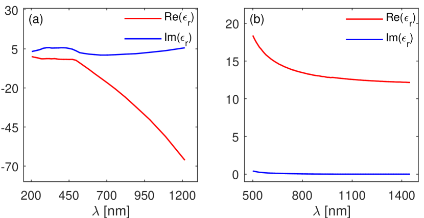
Figure 2: (a) Real and imaginary parts of the relative permittivity of gold. (b) The same as in (a), but corresponding to silicon.

3.1 Convergence of the numerical method

We begin the analysis of our numerical method with a study of its convergence characteristics. To this end, it should be noted that there are two main physical quantities that our numerical method is most suited to compute, namely scattering and absorption cross-sections, which are globally defined quantities, and the optical near-field, which is a local physical quantity. Therefore, analyzing the convergence of the calculations of these physical quantities will provide important information about both the global and local convergence properties of our numerical method.

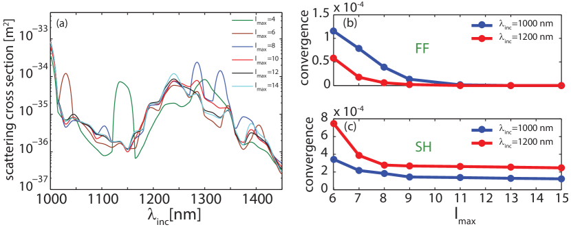
Figure 3: (a) Scattering cross-section calculated at the SH for a system of two silicon nanospheres with radius $R_{1}=R_{2}=$300\text{\,}\mathrm{nm}$$ and centers at $O_{1}(0,0,0)$ and $O_{2}(0,0,$800\text{\,}\mathrm{nm}$)$. (b) and (c) The error of the near-field, $\mathcal{E}_{l_{max}}^{\omega,\Omega}$, defined in (43), determined at the FF and SH frequency, respectively.

The system we used in testing the convergence of the method consists of two silicon nanospheres with radius $R_{1}=R_{2}=$300\text{\,}\mathrm{nm}$$ and centers at $O_{1}(0,0,0)$ and $O_{2}(0,0,$800\text{\,}\mathrm{nm}$)$. For this system, we calculated the SCS spectrum at the FF and SH, as well as the FF and SH electric fields in a grid of $M=2500$ points located in the $xy$-plane at $z=$400\text{\,}\mathrm{nm}$$, and covering the domain $[-400,400]\times[-400,400]~{}${\mathrm{nm}}^{2}$$. As the convergence properties of the linear TMM have been extensively studied, we focus here on the cross-sections at the SH (see Fig. 3a). Furthermore, the calculations were performed for increasing values of the cut-off of the orbital index, $l_{max}$, from $l_{max}=4$ up to $l_{max}=17$. In order to characterize the convergence of the near-field, we computed the norm

$$\mathcal{E}_{l_{max}}^{\omega,\Omega}=\frac{1}{M}\sqrt{\sum_{i=1}^{M}\left|\mathbf{E}_{l_{max}}^{\omega,\Omega}(\mathbf{r}_{i})-\mathbf{E}_{l_{max}=17}^{\omega,\Omega}(\mathbf{r}_{i})\right|^{2}},$$ (43)

and plotted the results in Fig. 3b (FF) and Fig. 3c (SH).

These results demonstrate that the calculation of both the SCS at the SH and the linear and nonlinear near-fields converge asymptotically as $l_{max}$ increases (note that the SCS at the FF converges much faster), which suggests both global and local convergence of the method. This is particularly important as it appears that the numerical method converges rather fast even for nanoparticles with relatively large index of refraction ($n_{Si}\simeq 3.45$), namely in a case when the near-field is strongly inhomogeneous.

3.2 Scattering from a single nanosphere

In the first example, we analyzed the linear and nonlinear scattering from a single gold nanosphere with radius $R=$200\text{\,}\mathrm{nm}$$ and a silicon nanosphere with radius $R=$300\text{\,}\mathrm{nm}$$, the calculated linear and nonlinear SCSs and ACSs being presented in Fig. 4. These cross-sections have been calculated both with the TMM and the FEM, so that we could further validate our numerical method. As it can be seen from Fig. 4, there is a good agreement between the spectra of the SCSs and ACSs, both at the FF and SH, calculated using our numerical method based on the TMM and the commercial FEM software.

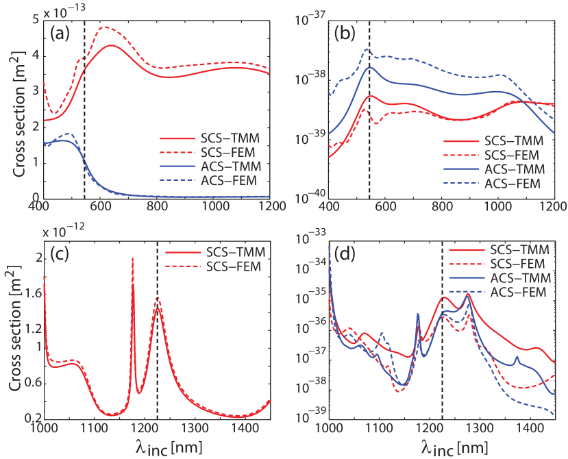
Figure 4: Scattering and absorption cross-sections calculated at the FF (left panels) and SH (right panels). The top and bottom panels correspond to a gold nanosphere with radius $R=$200\text{\,}\mathrm{nm}$$ and a silicon nanosphere with radius $R=$300\text{\,}\mathrm{nm}$$, respectively. The vertical lines indicate the input wavelengths at which the spatial profiles of the near-field are calculated.

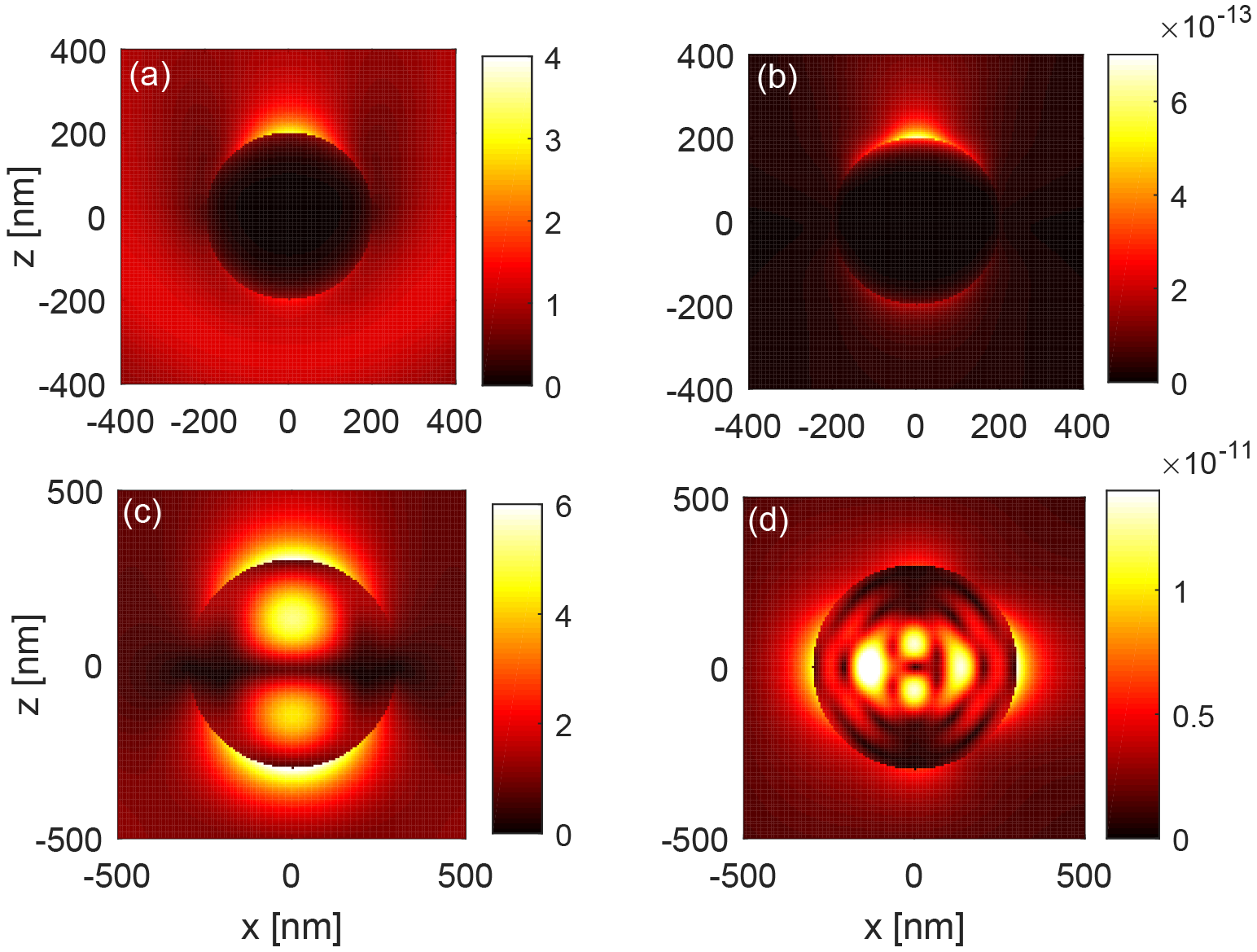
Figure 5: Spatial distribution of the electric field amplitude at the FF (left panels) and SH (right panels), calculated for a single gold nanosphere (top panels) at the incident wavelength $\lambda_{inc}=$545\text{\,}\mathrm{nm}$$ and for a single silicon nanosphere (bottom panels) at the incident wavelength $\lambda_{inc}=$1225\text{\,}\mathrm{nm}$$. The fields are determined in the $xz$-plane.

In the case of a single sphere, the TMM results are analytical, since the elements of the transfer matrix are equal to the Mie coefficients, which can be calculated analytically. Therefore, the discrepancy between the TMM and FEM results, especially notable in the SH regime, as per Figs. 4b and 4d, are perhaps due to the inaccuracies introduced by the discretization intrinsic to the FEM. More specifically, the electromagnetic field at the SH is strongly inhomogeneous and confined near the surface of the nanosphere, where the nonlinear polarization sources are located. This makes it difficult to be accurately resolved with finite elements. Moreover, approximately 25000 tetrahedral finite elements were used for a single frequency calculation both in the fundamental and second-harmonic case for gold and silicon spheres. By contrast, in our approach, only 390 VSWSs were needed, resulting in a significant memory reduction as compared to the FEM.

The spectra of the SCS of the gold nanosphere, at the FF and SH, show a pronounced maximum at the incident wavelengths $\lambda_{inc}=$640\text{\,}\mathrm{nm}$$ and $\lambda_{inc}=$545\text{\,}\mathrm{nm}$$, respectively. These spectral peaks are due to the excitation of localized surface plasmons on the metallic nanosphere, and are characterized by a large enhancement of the local optical field. In the case of the silicon sphere, the SCS spectrum at the FF has two peaks, which in this case correspond to electric dipole and magnetic dipole Mie resonances.

In Fig. 5 we present the spatial distribution of the amplitude of the electric field, $\lvert\mathbf{E}\rvert$, determined in the xz-plane, at both the FF (shown in Figs. 5a and 5c) and SH (shown in Figs. 5b and 5d). In the case of the gold sphere, the field profile is plotted at the incident wavelength $\lambda_{inc}=$545\text{\,}\mathrm{nm}$$ corresponding to the maximum in the SH scattering spectrum, whereas the field profile for the silicon sphere is computed at the incident wavelength $\lambda_{inc}=$1225\text{\,}\mathrm{nm}$$ and reveals the electric dipole character of the first resonance in the FF scattering spectrum. Moreover, it can be seen that the optical field does not penetrate into the gold sphere irrespective of the wavelength. In addition, unsurprisingly, the field at the SH is more inhomogeneous than at the FF, for both gold and silicon nanospheres.

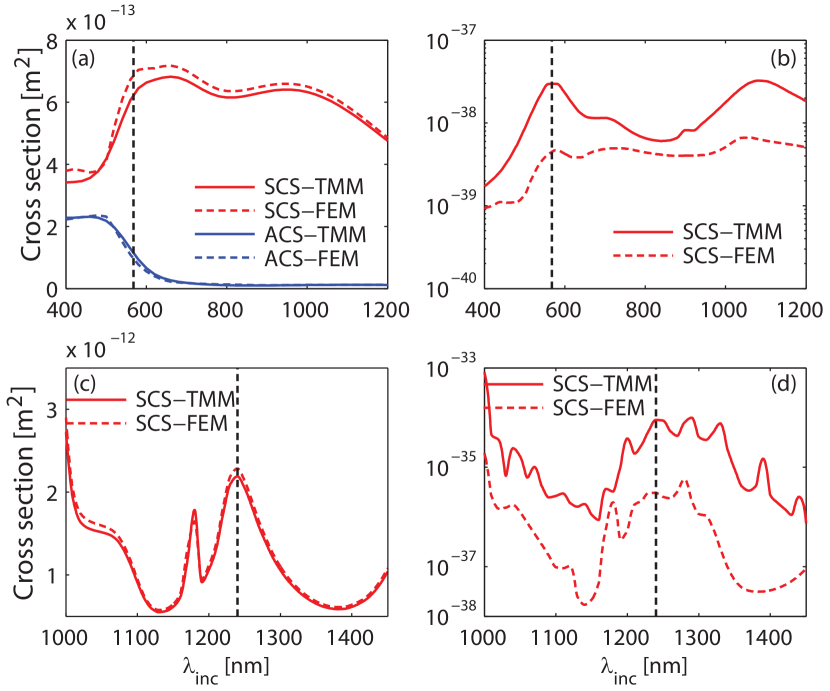
Figure 6: Scattering and absorption cross-section spectra at the FF (left panels) and SH (right panels). The top and bottom panels correspond to a gold nanodimer composed of two nanospheres with radii $R_{1}=$150\text{\,}\mathrm{nm}$$ and $R_{2}=$200\text{\,}\mathrm{nm}$$ centered in $O_{1}(0,0,0)$ and $O_{2}(0,0,$550\text{\,}\mathrm{nm}$)$, and for a silicon nanodimer composed of two identical spheres with radii $R_{1}=R_{2}=$300\text{\,}\mathrm{nm}$$ centered in $O_{1}(0,0,0)$ and $O_{2}(0,0,$800\text{\,}\mathrm{nm}$)$, respectively. The vertical lines indicate the input wavelengths at which the spatial profiles of the near-field are calculated.

3.3 Second-harmonic generation in nanodimers

Since in the case of a single sphere the translation-addition matrices are not employed, this is not a particularly challenging test for the full capabilities of the TMM. Therefore, in the second example, we analyze nanodimers made of gold and silicon nanospheres. In the case of the gold nanodimer, the spheres are centered at $O_{1}(0,0,0)$ and $O_{2}(0,0,$550\text{\,}\mathrm{nm}$)$, the corresponding radii being $R_{1}=$150\text{\,}\mathrm{nm}$$ and $R_{2}=$200\text{\,}\mathrm{nm}$$. The silicon nanodimer is composed of two identical spheres with radii $R_{1}=R_{2}=$300\text{\,}\mathrm{nm}$$, located at $O_{1}(0,0,0)$ and $O_{2}(0,0,$800\text{\,}\mathrm{nm}$)$. Finite-element method calculations have also been employed, using about 42000 tetrahedral elements for the gold dimer and 30000 elements for the silicon one. On the other hand, we used merely 780 VSWFs for the silicon and gold dimers. These examples are relevant for practical applications since strong near-fields can be generated in the space in-between the spheres, thus allowing for the design of highly sensitive sensing devices.

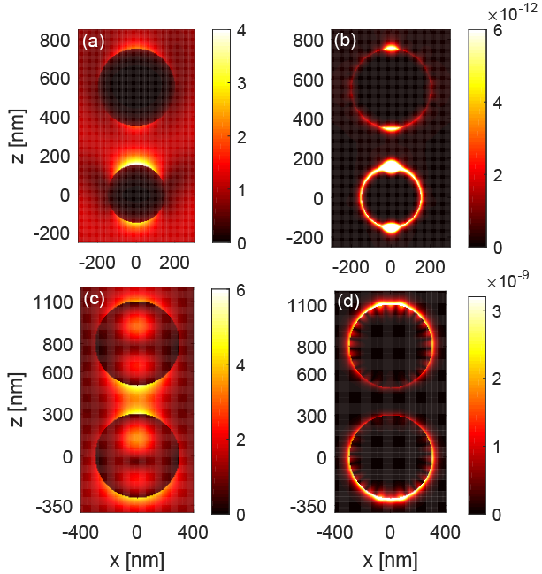
Figure 7: Spatial distribution of the electric field amplitude at the FF (left panels) and SH (right panels), calculated for the gold nanodimer (top panels) at the incident wavelength $\lambda_{inc}=$568\text{\,}\mathrm{nm}$$ and for the silicon nanodimer (bottom panels) at the incident wavelength $\lambda_{inc}=$1240\text{\,}\mathrm{nm}$$. The fields are determined in the $xz$-plane.

The spectrum of the SCS at the FF corresponding to the gold dimer shows a maximum at $\lambda_{inc}=$660\text{\,}\mathrm{nm}$$, whereas two peaks are observed in the spectrum of the SCS at the SH, at the incident wavelengths $\lambda_{inc}=$560\text{\,}\mathrm{nm}$$ and $\lambda_{inc}=$1080\text{\,}\mathrm{nm}$$. The SCS spectra of the silicon nanodimer have a more complex structure. In particular, in the linear regime, two spectral peaks are observed for incident wavelengths of similar values as those in the case of a single silicon nanosphere, but slightly redshifted due to inter-particle interactions (compare Fig. 4c and Fig. 6c). A similar situation is seen in the case of the SCS spectra at the SH. A series of spectral peaks can be observed, and again they are somewhat redshifted as compared to the case of a single silicon sphere (compare Fig. 4d and Fig. 6d). These spectral peaks are of plasmonic nature in the case of the gold dimer and originate from interacting Mie resonances in the case of the silicon dimer.

A perceptive reader has perhaps noticed that we did not present the nonlinear ACS spectra for the dimer cases. The main reason for this is that we found that they converge very slowly. This is explained by the fact that the ACS depends on the near-field, which is a physical quantity that converges very slowly, chiefly due to the inhomogeneous nature of the local field. To be more specific, the internal field expansion coefficients at the SH, $c_{n,\nu}^{\Omega}$ and $d_{n,\nu}^{\Omega}$, vary very slowly with the cut-off value of the orbital index, $l_{max}$, and therefore a large number of VSWFs must be included in the series expansion in order for the near-field (and consequently ACS) to converge. Moreover, we have noticed that when $l_{max}$ is very large, the entries of translation-addition matrices can become numerically unstable. Numerical errors introduced in the calculation of SH scattering field expansion coefficients are amplified when they are used to obtain internal SH field coefficients. This propagation of numerical errors particularly affects the SH absorption spectra of multiple nanospheres, and more so when their radii are smaller than the incident wavelength. Nevertheless, the physical quantity of practical interest is the SCS, as the power absorbed by clusters of particles is difficult to measure experimentally.

The spatial profile of the amplitude of the electric field computed in the xz-plane is shown in Fig. 7. In the case of the gold nanodimer, we choose the incident wavelength $\lambda_{inc}=$568\text{\,}\mathrm{nm}$$, namely at the location of the second peak in the SH spectrum of the SCS. In the silicon dimer case, we choose the wavelength $\lambda_{inc}=$1240\text{\,}\mathrm{nm}$$ to correspond to one of the Mie resonance wavelength. Interestingly enough, the field distribution corresponding to this latter case suggests that the resonance is a whispering-gallery mode [66].

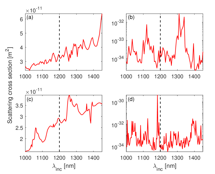
Figure 8: Scattering cross-section spectra at the FF (left panels) and SH (right panels). The top and bottom panels correspond to the centrosymmetric and non-centrosymmetric lattices, respectively. Spectra of absorption cross-sections at the FF are not plotted since the losses are negligible in this frequency range. The vertical line indicates the wavelength at which the field profile is calculated.

3.4 Second-harmonic generation in finite cubic lattices of nanospheres

In this example, we consider nanospheres arranged in two cubic lattices. We assume that the nanospheres in the two cubic lattices are made of silicon (a centrosymmetric material) and are located in the first octant of the Cartesian coordinate system, aligned with the $x$-, $y$- and $z$-axes. The first lattice contains $5\times 5\times 5=125$ identical nanospheres arranged so that the cluster is centrosymmetric. The second one is a non-centrosymmetric cubic array consisting of 8 zincblende unit cells containing a total of 95 spheres. This kind of crystal structure is found, for example, in GaAs or BAs, compounds widely used in the semiconductor industry. In the case of the centrosymmetric cluster, the nanospheres have the same radius, $R_{n}=$400\text{\,}\mathrm{nm}$$, $n=1,\ldots,125$, and are equally spaced with the center-to-center distance, $d=$850\text{\,}\mathrm{nm}$$, thus forming a cubic array with side length equal to $3.4\text{\,}\mathrm{\SIUnitSymbolMicro m}$. The non-centrosymmetric lattice contains two different sets of spheres: the first set contains larger spheres, with radius $R_{n}=$420\text{\,}\mathrm{nm}$$, $n=1,\ldots,63$, located at the vertices and side midpoints of the zincblende unit cells, whereas the other spheres have radius $r_{n}=$250\text{\,}\mathrm{nm}$$, $n=1,\ldots,32$ and are located inside the unit cells. The side length of this cluster is $4\text{\,}\mathrm{\SIUnitSymbolMicro m}$. We do not present here results of FEM calculations because for this problem the memory requirements are prohibitive. By contrast, in our TMM calculations we used 336 VSWFs per nanosphere, resulting in a total of 42000 basis functions for the centrosymmetric lattice and 31920 for the non-centrosymmetric one.

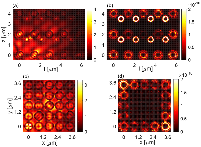
Figure 9: Distribution of the electric field amplitude at FF (left panels) and SH (right panels), calculated at $\lambda_{inc}=$1200\text{\,}\mathrm{nm}$$ for a non-centrosymmetric (top panels) and centrosymmetric (bottom panels) cluster of silicon nanospheres arranged in a cubic lattice. Top (bottom) panels correspond to the plane defined by the normal $(\hat{\mathbf{i}}-\hat{\mathbf{j}})/\sqrt{2}$ (the $xy$-plane bisecting the cluster through its center).

In Fig. 8 we plot the SCS spectra, at the fundamental and second-harmonic frequencies, for both types of lattices. It can be seen that they present an irregular aspect, which reflects an intricate interplay between the resonances of different spheres and their optical coupling. Moreover, the optical near-fields are presented in Fig. 9. Thus, in the upper panels of this figure, the fields are presented in the diagonal plane of the cluster defined by the normal $(\hat{\mathbf{i}}-\hat{\mathbf{j}})/\sqrt{2}$, whereas in the lower panels of this same figure, they are calculated in the $xy$-plane bisecting the structure through its center. These field profiles illustrate an important phenomenon related to the connection between the SHG properties and the symmetry characteristics of the cluster of spheres. Thus, as it can be observed in Figs. 9a and 9b, the optical field penetrates inside the non-centrosymmetric cluster both at the FF and SH frequency. By contrast, according to the lower panels of Fig. 9, in the case of the centrosymmetric cluster the fields are present inside the structure at FF only, whereas at the SH they are expelled from the cluster and are mainly concentrated at its outer boundary (see Fig. 9d). The reason for this is that the cluster in Figs. 9c and 9d is centrosymmetric and as such the (local) “bulk” second-order effective susceptibility cancels. The “surface” second-order effective susceptibility, however, has a nonzero value and therefore SH is generated at the surface of the cluster. By contrast, the structure formed from zincblende unit cells is non-centrosymmetric and thus the SHG is allowed in the bulk of the system, too.

3.5 Second-harmonic generation in an irregular distribution of nanospheres

The last example considered is the scattering from an irregular distribution of 11 silicon nanoparticles. This is a good test for the versatility of our algorithm, since there are no constraints imposed on the size and position of nanospheres. The only condition required to be fulfilled is that the spheres do not touch (see Fig. 10). In this example, we chose the nanospheres radii to be in the interval $R_{n}\in[$80\text{\,}\mathrm{nm}$,$310\text{\,}\mathrm{nm}$],n=1,\ldots,11$.

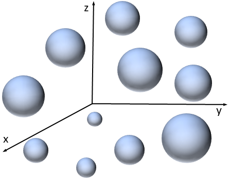
Figure 10: Schematics of the cluster of silicon nanoparticles, drawn at scale, considered in the last numerical example.

In Fig. 11 we show the SCS spectra of the ensemble of silicon nanospheres. Two peaks are revealed in the spectrum at the FF, one at $\lambda_{inc}=$1030\text{\,}\mathrm{nm}$$ and one at $\lambda_{inc}=$1215\text{\,}\mathrm{nm}$$ (as per Fig. 11a), whereas the SH SCS spectrum presents a much larger number of resonances (see Fig. 11b).

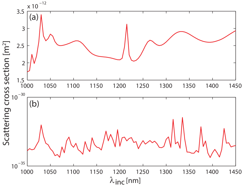
Figure 11: Spectra of scattering cross-section at the FF (a) and SH (b), computed for an irregular cluster of 11 silicon nanospheres. Spectra of absorption cross-section at the FF is not plotted since the losses are negligible in this frequency range.

4 Conclusion

In this article we have introduced a T-matrix method for fast and accurate electromagnetic wave scattering analysis of nanosphere clusters. Our numerical method can be used to characterize linear and nonlinear (second-harmonic) optical responses of the particle system. Different from previous studies, we include both surface and bulk contributions to the nonlinear polarization source. Following the classical T-matrix approach, the fields oscillating at fundamental frequency are expanded in a suitable set of vector spherical harmonics and the transfer matrix of the cluster is obtained by taking into account multiple wave scattering among the particles and linear boundary conditions on the boundaries of the nanospheres. After the fundamental field expansion coefficients are obtained, they are used in the computation of second-harmonic polarization sources. In the second step of our method, the SH T-matrix is formed by incorporating the mutual coupling between spheres at second-harmonic and nonlinear boundary conditions on their boundary-surfaces.

The proposed technique appears to have improved performance and lower memory imprint when compared to standard finite element method, while maintaining the overall accuracy in the scattering spectra. Furthermore, the algorithm lends itself to efficient parallelization on multi-core high-performance computer architectures since the submatrices representing the electromagnetic coupling between particles can be computed independently. This fact, along with state-of-the-art parallel iterative solvers, pave the way for fast and accurate numerical analysis of clusters containing thousands of nanoparticles.

Declaration of Competing Interest

The authors declare that they have no known competing financial interests or personal relationships that could have appeared to influence the work reported in this article.

CRediT authorship contribution statement

Ivan Sekulic: Methodology, Software, Investigation, Writing - original draft, review & editing. Jian Wei You: Methodology, Investigation, Writing - review & editing. Nicolae C. Panoiu: Conceptualization, Methodology, Writing - original draft, review & editing, Supervision.

Funding

This work was supported by the European Research Council (ERC) (Grant no. ERC-2014-CoG-648328).

Appendix A

In this Appendix we introduce the definition and main properties of vector spherical harmonics (VSHs) used in our study to represent the electromagnetic fields, as well as to expand the plane waves.

Definition of vector spherical wave functions

Given the unit vector $\hat{\mathbf{r}}=\mathbf{r}/r$, where $\mathbf{r}$ is the position vector of a point, $P$, we define three sets of mutually orthogonal VSHs: longitudinal VSHs, $\mathbf{Y}_{lm}$, which are oriented along $\hat{\mathbf{r}}$, and two sets of transverse VSHs, $\mathbf{X}_{lm}$ and $\mathbf{Z}_{lm}$, oriented perpendicular to $\hat{\mathbf{r}}$ [34, 56]. The triplet $\{\mathbf{X}_{lm},\mathbf{Y}_{lm},\mathbf{Z}_{lm}\}$ of VSHs form a right-handed system of vectors and are defined as:

$$\mathbf{Y}_{lm}(\theta,\phi)=Y_{lm}(\theta,\phi)\hat{\mathbf{r}},$$ (44a)

$$\mathbf{X}_{lm}(\theta,\phi)=\frac{1}{\sqrt{l(l+1)}}\hat{\mathbf{r}}\times\nabla_{\hat{\mathbf{r}}}Y_{lm}(\theta,\phi),$$ (44b)

$$\mathbf{Z}_{lm}(\theta,\phi)=\frac{1}{\sqrt{l(l+1)}}\nabla_{\hat{\mathbf{r}}}Y_{lm}(\theta,\phi).$$ (44c)

Furthermore, we define the regular VSWFs $\mathbf{M}_{lm}^{(1)}$ and $\mathbf{N}_{lm}^{(1)}$ as follows:

$$\mathbf{M}_{lm}^{(1)}(kr,\theta,\phi)=-j_{l}(kr)\mathbf{X}_{lm},$$ (45a)

$$\mathbf{N}_{lm}^{(1)}(kr,\theta,\phi)=\frac{1}{k}\nabla\times\mathbf{M}_{lm}^{(1)},$$ (45b)

$$\mathbf{M}_{lm}^{(1)}(kr,\theta,\phi)=\frac{1}{k}\nabla\times\mathbf{N}_{lm}^{(1)},$$ (45c)

where $k$ is the wave number calculated at the particular frequency in the medium of choice and $j_{l}(kr)$ are spherical Bessel functions of the first kind and order $l$. The radiative (outgoing) VSWFs $\mathbf{M}_{lm}^{(3)}$ and $\mathbf{N}_{lm}^{(3)}$ are defined by substituting the spherical Bessel functions in (45) with (outgoing) spherical Hankel functions, $h_{l}^{(1)}(kr)$, of the first kind and order $l$.

Scalar spherical harmonics can be defined in terms of associated Legendre functions $P_{l}^{m}$ as [56]:

$$Y_{lm}(\theta,\phi)=\gamma_{lm}\sqrt{l(l+1)}P_{l}^{m}(\cos\theta)e^{im\phi},$$ (46)

where $\gamma_{lm}$ is the normalization coefficient given by:

$$\gamma_{lm}=\sqrt{\frac{(2l+1)(l-m)!}{4\pi l(l+1)(l+m)!}}.$$ (47)

In these definitions the scalar spherical harmonic functions $Y_{lm}(\hat{\mathbf{r}})$ and the three kinds of VSHs are normalized to unity over a sphere:

$$\iint_{\Omega_{\hat{\mathbf{r}}}}Y_{lm}^{*}(\hat{\mathbf{r}})Y_{l^{\prime}m^{\prime}}(\hat{\mathbf{r}})d\Omega_{\hat{\mathbf{r}}}=\delta_{ll^{\prime}}\delta_{mm^{\prime}},$$ (48a)

$$\iint_{\Omega_{\hat{\mathbf{r}}}}\mathbf{A}_{lm}^{*}(\hat{\mathbf{r}})\cdot\mathbf{B}_{l^{\prime}m^{\prime}}(\hat{\mathbf{r}})d\Omega_{\hat{\mathbf{r}}}=\delta_{ll^{\prime}}\delta_{mm^{\prime}}\delta_{AB},$$ (48b)

where $\mathbf{A}$ and $\mathbf{B}$ can be any of the functions $\mathbf{X}$, $\mathbf{Y}$, and $\mathbf{Z}$.

Finally, the normalized VSHs can be defined in terms of associated Legendre functions as:

$$\mathbf{Y}_{lm}(\theta,\phi)=\gamma_{lm}\sqrt{l(l+1)}P_{l}^{m}(\cos\theta)e^{im\phi}\hat{\mathbf{r}},$$ (49a)

$$\mathbf{X}_{lm}(\theta,\phi)=\gamma_{lm}\left[-\frac{im}{\sin\theta}P_{l}^{m}(\cos\theta)e^{im\phi}\hat{\boldsymbol{\theta}}+\frac{d}{d\theta}P_{l}^{m}(\cos\theta)e^{im\phi}\hat{\boldsymbol{\phi}}\right],$$ (49b)

$$\mathbf{Z}_{lm}(\theta,\phi)=\gamma_{lm}\left[\frac{d}{d\theta}P_{l}^{m}(\cos\theta)e^{im\phi}\hat{\boldsymbol{\theta}}+\frac{im}{\sin\theta}P_{l}^{m}(\cos\theta)e^{im\phi}\hat{\boldsymbol{\phi}}\right].$$ (49c)

Expansion of plane waves in series of vector spherical wave functions

The series expansion of a plane wave in terms of WSVFs is given in (5a), with the expansion coefficients $q_{lm}^{\omega}$ and $p_{lm}^{\omega}$ calculated as follows [56]:

$$q_{lm}^{\omega} =-4\pi i^{l}\mathbf{X}_{lm}^{*}(\hat{\mathbf{k}}_{inc})\cdot\hat{\mathbf{e}}_{inc},$$ (50a)

$$p_{lm}^{\omega} =-4\pi i^{l+1}\mathbf{Z}_{lm}^{*}(\hat{\mathbf{k}}_{inc})\cdot\hat{\mathbf{e}}_{inc},$$ (50b)

where the symbol “$*$” denotes complex conjugation, $\hat{\mathbf{k}}_{inc}$ is the unit vector in the direction of the wave propagation, and $\hat{\mathbf{e}}_{inc}$ is the polarization direction of the plane wave.

Appendix B

In this Appendix, we introduce the boundary conditions for the electromagnetic fields, valid in the presence of a nonlinear surface polarization sheet, $\bm{\mathcal{P}}_{s}^{\Omega}(\mathbf{r})$, with support on a surface $\mathcal{S}$ separating two optical media. The interface is characterized by the normal, $\hat{\mathbf{n}}$, which we assume that points from medium $1$ to medium $2$. Then, the fields satisfy the following boundary conditions [58]:

$$\Delta\mathbf{E}_{\parallel}=-\frac{1}{\epsilon^{\prime}}\nabla_{S}\left[\hat{\mathbf{n}}\cdot\bm{\mathcal{P}}_{s}^{\Omega}(\mathbf{r})\right],\quad\mathbf{r}\in\mathcal{S},$$ (51a)

$$\Delta\mathbf{D}_{\perp}=-\nabla_{S}\cdot\bm{\mathcal{P}}_{s}^{\Omega}(\mathbf{r}),\quad\mathbf{r}\in\mathcal{S},$$ (51b)

$$\Delta\mathbf{H}_{\parallel}=i\Omega\hat{\mathbf{n}}\times\bm{\mathcal{P}}_{s}^{\Omega}(\mathbf{r}),\quad\mathbf{r}\in\mathcal{S},$$ (51c)

$$\Delta\mathbf{B}_{\perp}=0,\quad\mathbf{r}\in\mathcal{S},$$ (51d)

where $\Omega$ is the frequency, the symbol $\parallel$ ($\perp$) refers to the field component parallel (perpendicular) to the interface, $\nabla_{S}$ is the restriction of the operator $\nabla$ to the tangent plane, and, for a vector field $\mathbf{V}$, we defined $\Delta\mathbf{V}=\mathbf{V}_{2}-\mathbf{V}_{1}$, where $\mathbf{V}_{1}$ ($\mathbf{V}_{2}$) is the value of the field in medium $1$ ($2$) at a location infinitesimally close to the interface. Note that in deriving (51), one assumes that the fields depend on time as $e^{-i\Omega t}$. Using the fact that for a vector $\mathbf{V}$ the components tangent and perpendicular onto $\mathcal{S}$ are $\mathbf{V}_{\parallel}=-\hat{\mathbf{n}}\times\hat{\mathbf{n}}\times\mathbf{V}$ and $\mathbf{V}_{\perp}=(\hat{\mathbf{n}}\cdot\mathbf{V})\hat{\mathbf{n}}$, respectively, one can easily show that (51a) and (51c) with $\epsilon^{\prime}=\epsilon_{0}$ are equivalent to the boundary conditions (23).

References

• Mayer [2007] Maier SA. Plasmonics: Fundamentals and Applications. Springer; 2007.
• Boyd [1992] Boyd RW. Nonlinear Optics. Academic Press; 1992.
• Shen [2003] Shen YR. The Principles of Nonlinear Optics. Wiley; 2003.
• Kauranen [2012] Kauranen M, Zayats AV. Nonlinear plasmonics. Nat Photonics 2012;6:737-48.
• Butet [2015] Butet J, Brevet PF, Martin OJF. Optical second harmonic generation in plasmonic nanostructures: from fundamental principles to advanced applications. ACS Nano 2015;9:10545-62.
• Panoiu [2018] Panoiu NC, Sha WEI, Lei DY, Li GC. Nonlinear optics in plasmonic nanostructures. J Opt 2018;20:083001.
• Cao [2002] Cao YWC, Jin RC, Mirkin CA. Nanoparticles with Raman Spectroscopic Fingerprints for DNA and RNA Detection. Science 2002;297:1536-10.
• Homola [2008] Homola J, Surface plasmon resonance sensors for detection of chemical and biological species. Chem Rev 2008;108:462-93.
• Pendry [1999] Pendry JB, Holden AJ, Robbins DJ, Stewart WJ. Magnetism from conductors and enhanced nonlinear phenomena. IEEE Trans Microw Theory Tech 1999;47:2075-84.
• Liu [2008] Liu N, Guo H, Fu L, Kaiser S, Schweizer H, Giessen H. Three-dimensional photonic metamaterials at optical frequencies. Nat Mater 2008;7:31-37.
• Ziolkowski [2004] Ziolkowski RW. Propagation in and scattering from a matched metamaterial having a zero index of refraction. Phys Rev E 2004;70:046608.
• Bloembergen [1968] Bloembergen N, Chang RK, Jha SS, Lee CH. Optical second-harmonic generation in reflection from media with inversion symmetry. Phys Rev 1968;174,813-22.
• Bozhevolny [2003] Bozhevolnyi SI, Beermann J, Coello V. Direct observation of localized second-harmonic enhancement in random metal nanostructures. Phys Rev Lett 2003;90:197403.
• Cao2 [2007] Cao L, Panoiu NC, Osgood RM. Surface second-harmonic generation from surface plasmon waves scattered by metallic nanostructures. Phys Rev B 2007;75:205401.
• Cao3 [2009] Cao L, Panoiu NC, Bhat RDR, Osgood RM. Surface second-harmonic generation from scattering of surface plasmon polaritons from radially symmetric nanostructures. Phys Rev B 2009;79:235416.
• Timbrell [2018] Timbrell D, You JW, Kivshar YS, Panoiu NC. A comparative analysis of surface and bulk contributions to second-harmonic generation in centrosymmetric nanoparticles. Sci Rep 2018;8:3586.
• Dadap1 [1999] Dadap JI, Shan J, Eisenthal KB, Heinz TF. Second-harmonic Rayleigh scattering from a sphere of centro-symmetric material. Phys Rev Lett 1999;83:4045.
• Pavlyukh [2004] Pavlyukh Y, Hubner W. Nonlinear Mie scattering from spherical particles. Phys Rev B 2004;70:245434.
• Forestiere1 [2014] Capretti A, Forestiere C, Dal Negro L, Miano G. Full-wave analytical solution of second-harmonic generation in metal nanospheres. Plasmonics 2014;9:151-66.
• Beer1 [2007] de Beer AGF, Roke S. Nonlinear Mie theory for second-harmonic and sum-frequency scattering. Phys Rev B 2007;75:245438.
• Silvester [1996] Silvester PP, Ferrari RL. Finite Elements for Electrical Engineers. Cambridge University Press; 1996.
• Jin [2002] Jin JM. The Finite Element Method in Electromagnetics. John Wiley & Sons; 2002.
• Yee [1966] Yee K. Numerical solution of initial boundary value problems involving Maxwellโ€™s equations in isotropic media. IEEE Trans Antennas Propag 1966;14(8):302-7.
• Taflove [2005] Taflove A, Hagness SC. Computational Electrodynamics: The Finite-Difference Time-Domain Method. Artech House; 2005.
• Mayergoyz [2005] Mayergoyz ID, Fredkin DR, Zhang Z. Electrostatic (plasmon) resonances in nanoparticles. Phys Rev B 2005;72:155412.
• Hohenester1 [2005] Hohenester U, Krenn J. Surface plasmon resonances of single and coupled metallic nanoparticles: A boundary integral method approach. Phys Rev B 2005;72:195429.
• Myroshnychenko [2008] Myroshnychenko V, Rodriguez-Fernandez J, Pastoriza-Santos I, Funston AM, Novo C, Mulvaney P, Liz-Marzan LM, Garcia de Abajo FJ. Modeling the optical response of gold nanoparticles. Chem Soc Rev 2008;37:1792-805.
• Harrington [1968] Harrington RF. Field Computation by Moment Method. Macmillan; 1968.
• Waterman1 [1965] Waterman PC. Matrix formulation of electromagnetic scattering. Proc IEEE 1965;53(8):805-12.
• Waterman2 [1969] Waterman PC. Scattering by dielectric obstacles. Alta Freq 1969;38:348-52.
• Barber [1975] Barber P, Yeh C. Scattering of electromagnetic waves by arbitrarily shaped dielectric bodies. Appl Opt 1975;14(12):2864-72.
• Peterson [1973] Peterson B, Strom S. T-matrix for electromagnetic scattering from an arbitrary number of scatterers and representations of E(3). Phys Rev D 1973;8:3661-78.
• Schatz [2017] Heaps CW, Schatz GC. Modeling super-resolution SERS using a T-matrix method to elucidate molecule-nanoparticle coupling and the origins of localization errors. J Phys Chem 2017;146:224201.
• Varshalovich [1988] Varshalovich DA, Moskalev AN, Khersonskii VK. Quantum Theory of Angular Momentum. World Scientific Publishing; 1988.
• Jackson [1999] Jackson JD. Classical Electrodynamics. John Wiley & Sons; 1999.
• Mishchenko1 [1996] Mishchenko MI, Travis LD, Mackowski DW. T-matrix computations of light scattering by nonspherical particles: a review. J Quant Spectrosc Radiat Transfer 1996;55:535-75.
• Mishchenko1 [2007] Mishchenko MI, Videen G, Babenko VA, Khlebtsov NG, Wriedt T. Comprehensive T-matrix reference database: A 2004-06 update. J Quant Spectrosc Radiat Transfer 2007;106:304-24.
• Schatz [2010] Chen H, McMahon JM, Ratner MA, Schatz GC. Classical electrodynamics coupled to quantum mechanics for calculation of molecular optical properties: a RT-TDDFT/FDTD approach. J Phys Chem C 2010;114:14384-92.
• Hohenester1 [2015] Hohenester U. Quantum corrected model for plasmonic nanoparticles: A boundary element method implementation. Phys Rev B 2015;91:205436.
• Deng [2018] Deng H, Manrique DZ, Chen X, Panoiu NC, Ye F. Quantum mechanical analysis of nonlinear optical response of interacting graphene nanoflakes. APL Photonics 2018;3:016102.
• You [2019] You JW, Panoiu NC. Analysis of the Interaction Between Classical and Quantum Plasmons via FDTD-TDDFT Method. IEEE J Multiscale Multiphys Comput Tech 2019;4:111-8.
• Makitalo [2011] Makitalo J, Suuriniemi S, Kauranen M. Boundary element method for surface nonlinear optics of nanoparticles. Opt Express 2011;19:23386-99.
• Forestiere2 [2013] Forestiere C, Capretti A, Miano G. Surface integral method for second harmonic generation in metal nanoparticles including both local-surface and nonlocal-bulk sources. J Opt Soc Am B 2013;30(9):2355-64.
• Song [1997] Song J, Lu CC, Chew WC. Multilevel fast multipole algorithm for electromagnetic scattering by large complex objects. IEEE Trans Antennas Propag 1997; 45(10):1488-93.
• Bebendorf [2000] Bebendorf M. Approximation of boundary element matrices. Numer Math 2000;86:565-89.
• Biris [2010] Biris CG, Panoiu NC. Second harmonic generation in metamaterials based on homogeneous centrosymmetric nanowires. Phys Rev B 2010;81:195102.
• BirisBis [2010] Biris CG, Panoiu NC. Nonlinear pulsed excitation of high-Q optical modes of plasmonic nanocavities. Opt Express 2010;18:17165-79.
• Xu [2012] Xu J, Zhang X. Second harmonic generation in three-dimensional structures based on homogeneous centrosymmetric metallic spheres. Opt Express 2012;20(2):1668-84.
• Mie [1908] Mie G. Beitrage zur optik trรผber medien, speziell kolloidaler metallรถsungen. Ann Phys (Berl) 1908;330(3):377โ€445.
• Forestiere3 [2011] Forestiere C, Iadarola G, Dal Negro L, Miano G. Near-field calculation based on the T-matrix method with discrete sources. J Quant Spectrosc Radiat Transfer 2011;112:2384-94.
• Tsang [1985] Tsang L, Kong JA, Shin RT. Theory of Microwave Remote Sensing. Wiley; 1985.
• Sekulic [2019] Sekulic I, Tzarouchis DC, Ylรค-Oijala P, Ubeda E, Rius JM. Enhanced discretization of surface integral equations for resonant scattering analysis of sharp-edged plasmonic nanoparticles. Phys Rev B 2019;99:165417.
• Cruzan [1962] Cruzan OR. Translational addition theorems for spherical vector wave functions. Quart Appl Math 1962;20:33-40.
• Mackowski [1996] Mackowski DW, Mishchenko MI. Calculation of the T-matrix and the scattering matrix for ensembles of spheres. J Opt Soc Am A 1996;13:2266-78.
• Stout1 [2002] Stout B, Auger JC, Lafait J. A transfer matrix approach to local field calculations in multiple-scattering problems. J Mod Opt 2002;49:2129-52.
• Stout2 [2001] Stout B, Auger JC, Lafait J. Individual and aggregate scattering matrices and cross-sections: conservation laws and reciprocity. J Mod Opt 2001;48:2105-28.
• Sipe1 [1980] Sipe JE, So VCY, Fukui M, Stegeman GI. Analysis of second-harmonic generation at metal surfaces. Phys Rev B 1980;21:4389-402.
• Heinz [1991] Heinz TF. Nonlinear Surface Electromagnetic Phenomena. Elsevier; 1991.
• [59] CST Studioยฎ, www.cst.com.
• Johnson [1972] Johnson PB, Christy RW. Optical constants of the noble metals. Phys Rev B 1972;6:4370-79.
• Schinke [2015] Schinke C, Peest PC, Schmidt J, Brendel R, Bothe K, Vogt MR, Kroger I, Winter S, Schirmacher A, Lim S, Nguyen HT, MacDonald D. Uncertainty analysis for the coefficient of band-to-band absorption of crystalline silicon. AIP Advances 2015;5:067168.
• Corvi [1986] Corvi M, Schaich W. Hydrodynamic-model calculation of second-harmonic generation at a metal surface. Phys Rev B 1986;33:3688-95.
• Guyot [1986] Guyot-Sionnest P, Chen W, Shen YR. General considerations on optical second-harmonic generation from surfaces and interfaces. Phys Rev B 1986;33:8254-63.
• Rudnick [1971] Rudnick J, Stern EA. Second-harmonic radiation from metal surfaces. Phys Rev B 1971;4:4274-90.
• Falasconi [2001] Falasconi M, Andreani LC, Malvezzi AM, Patrini M, Mulloni V, Pavesic L. Bulk and surface contributions to second-order susceptibility in crystalline and porous silicon by second-harmonic generation. Surf Sci 2011;481:105-12.
• Biris [2013] Biris CG, Panoiu NC. Nonlinear Surface-Plasmon Whispering-Gallery Modes in Metallic Nanowire Cavities. Phys Rev Lett 2013;111:203903.