A Mathematical Principle of Deep Learning: Learn the Geodesic Curve in the Wasserstein Space

Abstract

Recent studies revealed the mathematical connection of deep neural network (DNN) and dynamic system. However, the fundamental principle of DNN has not been fully characterized with dynamic system in terms of optimization and generalization. To this end, we build the connection of DNN and continuity equation where the measure is conserved to model the forward propagation process of DNN which has not been addressed before. DNN learns the transformation of the input distribution to the output one. However, in the measure space, there are infinite curves connecting two distributions. Which one can lead to good optimization and generaliztion for DNN? By diving the optimal transport theory, we find DNN with weight decay attempts to learn the geodesic curve in the Wasserstein space, which is induced by the optimal transport map. Compared with plain network, ResNet achieves better approximation to the geodesic curve, which explains why ResNet can be optimized and generalize better. Numerical experiments show that the data tracks of both plain network and ResNet tend to be line-shape in term of line-shape score (LSS), and the map learned by ResNet is closer to the optimal transport map in term of optimal transport score (OTS). In a word, we conclude a mathematical principle of deep learning is to learn the geodesic curve in the Wasserstein space; and deep learning is a great engineering realization of continuous transformation in high-dimensional space.

Keywords: Deep learning, deep neural network, ResNet, continuity equation, optimal transport, optimization, generalization

Significance Though the performance of deep learning is excellent in various aspects, it is still not well understood. To address this issue, we discover that deep neural network (DNN) tends to approximate the geodesic curve in the Wasserstein space in the training process. The degree of approximation is positively correlated with the performance of DNN. Compared with plain network, ResNet approximates the geodesic curve better theoretically, which illustrates why ResNet can be deeper and have better generalization ability. Numerical experiments support our findings in term of line-shape score and optimal transport score, which are designed to measure the degree of approximation.

1 Introduction

Deep neural network (a.k.a. deep learning) has become a very powerful tool in many fields including computer vision, natural language processing, bioinformatics and so on. However, for tasks with security needs, DNN is not trustful enough due to its black box internals. DNN is hard to analyze because the composition of activation functions (e.g., ReLU) leads to nonlinearity and nonconvexity. Nevertheless, some studies have provided insights and interpretation into DNN by constructing new models such as neural tangent kernel [2][1][6][14][21][20][30][34][51] and deep linear network [37][7][19][38][33]; or by generalizing existing machine learning techniques such as matrix decomposition and sparse coding to multi-layer ones [46][5][25][40][36]. These ideal models simplify the settings of DNN and obtain corresponding theoretical results.

There were also several studies focusing on explaining advanced DNN models such as ResNet [28] and its variants [47][29][44], which have attracted great attentions to their extreme depth. They have attempted to interpret ResNet from different angles such as the unraveled view [41], the unrolled iterative estimation view [24][31], the multi-layer convolutional sparse coding view [49] and the dynamic system view [26][43]. However, the superiority of ResNet over plain network has not been fully explained theoretically.

In computer science, the continuous concept are realized through discretization. Inversely, to analyze DNN theoretically, one can assume: (1) the data points are sampled from a continuous distribution; (2) the layerwise transformation in DNN can be viewed as a discrete approximation to the continuous curve in the probability measure space $\mathcal{P}(\mathbb{R}^{d})$, which can be described with a dynamic system. Haber and Ruthotto [26] and E [43] first interpreted DNN with ordinary differential equations (ODEs). Wang et al. [42] built the connection of ResNet and transport equation (TE) to investigate the data flow in both forward and backward propagation. However, since the proportion of data points in certain classes are fixed in representation space of different levels, ODE and TE fail to model the conservation of probability in the forward propagation process of DNN.

Figure 1: Illustration of DNN to learn the geodesic curve in the Wasserstein space. (A) In the measure space $\mathcal{P}(\mathbb{R}^{d})$, there are infinite curves connecting $\mu_{0}$ and $\mu_{1}$ which satisfy continuity equations in (1). (B) DNN is a discretization to a continuous curve. The vector fields $\tilde{v}_{0},\tilde{v}_{h},\cdots,\tilde{v}_{(n-1)h}$ are learned by shallow networks, where $h=\frac{1}{n}$. Then we obtain a polyline connecting $\tilde{\mu}_{0},\tilde{\mu}_{h},\cdots,\tilde{\mu}_{(n-1)h},\tilde{\mu}_{1}$.(C) The data points are forward propagated through a straight line inside DNN of four layers according to the geodesic curve induced by the optimal transport map. (D) The red arrows indicate that the data tracks have the tendency to deviate from the straight line from the data $x^{(0)}$ to its representation $x^{(4)}$. The green arrows indicate that weight decay in DNN can draw the tracks to the straight line. (E) Two data tracks intersect or close, then the two data points tend to be indistinguishable by adding a noise. (F) Two data points even with noise can be well discriminated, when the data tracks are organized in the way of an optimal transport map.

To address this issue, we utilized the curves satisfying continuity equations which conserve the measure of distributions to model DNN (Fig. 1A). Among all the curves, the geodesic one in the Wasserstein space $(\mathcal{P}_{2}(\mathbb{R}^{d}),W_{2})$ has very good properties which can benefit the optimization and generalization of DNN. DNN can be considered as a layerwise transformation to approximate the continuous transformation from $\mu_{0}$ and $\mu_{1}$ which denote the continuous distributions corresponding to the data and its representations respectively (Fig. 1B). According to the Benamou-Brenier formula [12], the approximation of DNN and the geodesic curve can be achieved by minimizing an energy function which is upper bounded by weight decay. Thus, DNN has two characteristics (Fig. 1C): (1) the data tracks of layerwise transformation in DNN tend to be line-shape; (2) the map learned by DNN is close to an optimal transport map.

Compared with plain network, ResNet is a better approximation to the geodesic curve according to the forward Euler method. Then we can explain why ResNet can be deeper, why ResNet generalizes better and why ResNet is harder to attack, compared with plain network. First, the data tracks in ResNet tend to be more line-shape than those in plain network though both of them likely zigzag due to the back propagation (BP) algorithm (Fig. 1D). We demonstrate the optimization process is more effective along a straight line than a zigzag track. Thus, ResNet can overcome the degradation problem and achieve lower loss by employing more layers. Second, since the map learned by ResNet is closer to optimal transport map, the distance of two tracks is lower bounded. Thus, ResNet does not tend to mix up two tracks when adding noise (Fig. 1E and Fig. 1F), which leads to better generalization compared to plain network.

Numerical experiments show that the data tracks of both plain network and ResNet tend to be line-shape in term of line-shape score (LSS), and the map learned by ResNet is closer to the optimal transport map in term of optimal transport score (OTS). Moreover, LSS and OTS are closely related with the performance of both plain network and ResNet, suggesting their principle is indeed to learn the geodesic curve in the Wasserstein space.

2 Methodology

In the forward propagation, DNN may increase the dimension of data or representation to obtain more relevant information and reduce the dimension to abstract better representation. When the network is very deep, sequential layers may not change the dimension of representations (e.g., ResNet). In this section, we first assume the output dimension of DNN is the same as the input one to derive the connection of DNN and the geodesic curve in the Wasserstein space and then discuss the generalization to dimension-varying situations in subsection 2.5.

2.1 Connection of DNN and the continuity equation

In the following, we illustrate the connection of DNN with the same input and output dimensions and continuous curve in the probability measure space $\mathcal{P}(\mathbb{R}^{d})$. Let $(\mu_{t})$ be an absolutely continuous curve in $\mathcal{P}(\mathbb{R}^{d})$. According to Theorem 2.29 in [3], there exists a Borel family of vector fields $v_{t}$ on $\mathbb{R}^{d}$ such that the continuity equation

$$\frac{d}{dt}\mu_{t}+\nabla\cdot(v_{t}\mu_{t})=0,$$ (1)

holds in the sense of distributions. The continuity equation describes the link between the motion of the continuum $\mu_{t}$ and the instantaneous velocity $v_{t}:\mathbb{R}^{d}\to\mathbb{R}^{d}$ of every “atom” of $\mu_{t}$. It is therefore natural to think at the vector field $v_{t}$ as the infinitesimal variation of the continuum $\mu_{t}$. If we discretize the continuity equation with $t\in[0,1]$, then for $h=\frac{1}{n}$, we have

$$\tilde{\mu}_{(i+1)h}=(I_{d}+h\tilde{v}_{ih})_{\#}\tilde{\mu}_{ih},\quad i=0,1,\cdots,n-1,$$ (2)

where $I_{d}$ denotes the identity map, $\tilde{\mu}_{ih}\ (i=0,1,\cdots,n-1)$ are points on the curve $(\mu_{t})$. Since $h$ can be absorbed in $\tilde{v}_{ih}$, we directly use $\tilde{v}_{i}$ in place of $h\tilde{v}_{ih}$. The layerwise maps in DNN induce a vector field corresponding to $I_{d}+\tilde{v}_{i}$. For instance, in plain network, $I_{d}+\tilde{v}_{i}$ corresponds to a single layer map. While in ResNet, the vector field $\tilde{v}_{i}$ is specifically induced by a shallow network and $I_{d}$ is modeled by skip connection. This makes ResNet a better approximation to $I_{d}+\tilde{v}_{i}$ compared to plain network. Thus, stacking all the layers of plain network or ResNet blocks can be regarded as a discrete and measure preserving approximation to the continuity equation (Fig. 1B).

2.2 Geodesic curve in the Wasserstein space

When $\mu_{0}$ and $\mu_{1}$ are fixed, there are infinite curves in the probability measure space connecting $\mu_{0}$ and $\mu_{1}$, each of which can be approximated by a discretized DNN. However, not all the networks can be optimized or generalize well (see Section 3 and 4 in detail). From optimization perspective, the efficiency of the BP algorithm varies for different curves. A basic assumption of deep learning is that a data or representation distribution locates on a continuous manifold. Thus, from generalization perspective, the model should not only fit the training data, but also generalize to the region surrounding it.

Among all the curves, the geodesic one in the Wasserstein space have very good properties. It is induced by the optimal transport map $T$ from a distribution $\mu_{0}$ to another distribution $\mu_{1}$ with the minimum cost. This cost is termed as the Wasserstein distance $W(\mu_{0},\mu_{1})$, i.e.

$$W_{c}(\mu_{0},\mu_{1})=\inf_{T_{\#}\mu_{0}=\mu_{1}}\int c\left(x,T\left(x\right)\right)d\mu_{0}\left(x\right),$$ (3)

where $c(\cdot,\cdot)$ is the cost function of moving each unit mass from the source $\mu_{0}$ to the target $\mu_{1}$. In this paper, $c\left(x,T\left(x\right)\right)$ is set to $\|x-T(x)\|_{2}^{2}$, which is commonly used in both optimal transport and deep learning. The Wasserstein distance with respect to this $L_{2}$ norm denoted by $W_{2}$ is indeed a distance metric on $\mathcal{P}(\mathbb{R}^{d})$. Moreover, $\forall\mu_{0},\mu_{1}\in(\mathcal{P}_{2}(\mathbb{R}^{d}),W_{2})$, there is a constant speed geodesic curve ($\mu_{t}$) connecting $\mu_{0}$ and $\mu_{1}$ such that

$$W_{2}(\mu_{t},\mu_{s})=|t-s|W_{2}(\mu_{0},\mu_{1}),\quad\forall t,s\in[0,1].$$ (4)

The constant speed geodesic curve ($\mu_{t}$) is induced by the optimal transport map $T$, i.e.

$$\mu_{t}=\left(\left(1-t\right)I_{d}+tT\right)_{\#}\mu_{0}.$$ (5)

Since ($\mu_{t}$) satisfies the continuity equation (1), the construction of ($\mu_{t}$) in (5) results in the specific structure of the vector field $(v_{t})$. For $\psi\in C^{\infty}(\mathbb{R^{d}})$, it holds

$$\frac{d}{dt}\int\psi d\mu_{t} =\frac{d}{dt}\int\psi((1-t)I_{d}+tT)d\mu_{0}$$ (6)

$$=\int\left\langle\nabla\psi((1-t)I_{d}+tT),T-I_{d}\right\rangle d\mu_{0}$$

$$=\int\left\langle\nabla\psi,(T-I_{d})\circ\left(\left(1-t\right)I_{d}+tT\right)^{-1}\right\rangle d\mu_{t}.$$

Then by taking

$$v_{t}:=(T-I_{d})\circ((1-t)I_{d}+tT)^{-1},$$ (7)

we obtain the continuity equation corresponding to $(\mu_{t})$.

2.3 Weight decay leads to approximation to the geodesic curve

However, it is not easy to impose the constraint induced by (7) on $\tilde{v}_{i}$ directly, because in the training process of DNN, we actually don’t know $T$. Also it is intractable to force $\tilde{v}_{i}$ to satisfy (7) since it has too many parameters. Alternatively, the following proposition transforms this constraint to an energy function minimization problem.

Proposition 1

(Benamou-Brenier formula[12]) Let $\mu_{0}$, $\mu_{1}\in\mathcal{P}(\mathbb{R}^{d})$. Then it holds

$$W_{2}\left(\mu_{0},\mu_{1}\right)=\inf\left\{\int_{0}^{1}\left\|v_{t}\right\|_{L^{2}(\mu_{t})}dt\right\},$$ (8)

where the infimum is taken among all weakly continuous distributional solutions of the continuity equation $(\mu_{t},v_{t})$ connecting $\mu_{0}$ and $\mu_{1}$.

We can pursue the discretization of the curve induced by the optimal transport map through minimizing the $L_{2}$ norm of $\tilde{v}_{i}$ on $\tilde{\mu}_{ih}$ for all $i$

$$\min_{\tilde{v}_{i}}\quad\sum_{i=0}^{n-1}\|\tilde{v}_{i}\|_{L^{2}(\tilde{\mu}_{ih})}$$ (9)

$$\mbox{s.t.}\left\{\begin{aligned} &\tilde{\mu}_{0}=\mu_{0},\\ &\tilde{\mu}_{(i+1)h}=(I_{d}+\tilde{v}_{i})_{\#}\tilde{\mu}_{ih},\ i=0,1,\cdots,n-1,\\ &\tilde{\mu}_{1}=\mu_{1}.\\ \end{aligned}\right.$$

Actually, $\|\tilde{v}_{i}\|_{L^{2}(\tilde{\mu}_{ih})}$ is upper bounded by the weight decay, which is a crucial ingredient of DNN. For instance, since the vector field is induced by a shallow network in ResNet, let $\tilde{v}_{i}(\cdot)=W_{i}^{(2)}\sigma(W_{i}^{(1)}\sigma(\cdot))$, where $W_{i}^{(1)},W_{i}^{(2)}$ are $d\times d$ weight matrices and $\sigma(\cdot)$ is the ReLU activation function. Then we have

$$\|\tilde{v}_{i}\|_{L^{2}(\tilde{\mu}_{ih})} =\int\|W_{i}^{(2)}\sigma(W_{i}^{(1)}\sigma(x))\|_{2}^{2}d\tilde{\mu}_{ih}(x)$$ (10)

$$\leq\|W_{i}^{(2)}\|_{F}^{2}\|W_{i}^{(1)}\|_{F}^{2}\int\|x\|_{2}^{2}d\tilde{\mu}_{ih}(x)$$

$$\leq\frac{1}{4}\left(\|W_{i}^{(2)}\|_{F}^{2}+\|W_{i}^{(1)}\|_{F}^{2}\right)^{2}\int\|x\|_{2}^{2}d\tilde{\mu}_{ih}(x).$$

It is natural to assume that in the training process of DNN with a weight decay that $\|W_{i}^{(1)}\|_{F}^{2}$, $\|W_{i}^{(2)}\|_{F}^{2}$ and $\int\|x\|_{2}^{2}d\tilde{\mu}_{ih}(x)$ are upper bounded. Then in the training process, there exist $C$ such that

$$\sum_{i=0}^{n-1}\|\tilde{v}_{i}\|_{L^{2}(\mu_{ih})}\leq C\sum_{i=0}^{n-1}\left(\|W_{i}^{(1)}\|_{F}^{2}+\|W_{i}^{(2)}\|_{F}^{2}\right).$$ (11)

The right side of (11) coincides with the weight decay. For plain network, let $(I_{d}+\tilde{v}_{i})(\cdot)=\sigma(W^{(i)}\cdot)$, similar result holds

$$\sum_{i=0}^{n-1}\|\tilde{v}_{i}\|_{L^{2}(\tilde{\mu}_{ih})} =\sum_{i=0}^{n-1}\int\|\sigma\left(W^{(i)}x\right)-x\|_{2}^{2}d\tilde{\mu}_{ih}(x)$$ (12)

$$\leq\sum_{i=0}^{n-1}\int\left(\|W^{(i)}\|_{F}^{2}\|x\|_{2}^{2}+\|x\|_{2}^{2}\right)d\tilde{\mu}_{ih}(x)$$

$$\leq C^{{}^{\prime}}\sum_{i=0}^{n-1}\|W^{(i)}\|_{F}^{2},$$

where $C^{{}^{\prime}}$ is a constant correlated with $\int\|x\|_{2}^{2}d\tilde{\mu}_{ih}(x)$.

We denote $:\mathbb{R}^{d}\to\mathbb{R}^{d}$ as the map learned by stacking $n$ layers of plain network or $n$ ResNet blocks, i.e.

$$f=(I_{d}+\tilde{v}_{n-1})\circ(I_{d}+\tilde{v}_{n-2})\cdots\circ(I_{d}+\tilde{v}_{0}).$$ (13)

Let $\mathcal{L}(f,\theta)$ be the loss function of a certain task with respect to $f$, $\theta$ denotes the parameters in the objective function which does not belong to $f$. Then the problem of solving the task with DNN can be formulated as

$$\min_{f,\theta}\mathcal{L}(f,\theta)+\gamma\sum_{W\in\operatorname{Para}\{f\}}\|W\|_{F}^{2},$$ (14)

where $\gamma$ is the hyperparameter to balance the two terms in the objective function and $\operatorname{Para}\{f\}$ denotes the set of weight matrices in $f$. The output distribution of $f$ has degree of freedom to change with respect to $\theta$, while $\mathcal{L}(f,\theta)$ doesn’t increase. By adding the regularizer, at the end of the training process, the model simultaneously achieves: (1) a map which can solve the task with low loss; (2) a discrete approximation to a curve from the input distribution to the output distribution of $f$ which is close to the geodesic curve induced by the optimal transport map.

2.4 Connection to Helmoltz decomposition

With the exist of $\mathcal{L}(f,\theta)$, $f$ can not be optimal transport map absolutely. Nevertheless, $f$ can be decomposed into two maps, one of which is the optimal transport map.

Proposition 2

(Brenier’s polar factorization[13]) Suppose $\mu_{0}$ is absolutely continuous with respect to Lebesgue measure, and $f:\mathbb{R}^{d}\to\mathbb{R}^{d}$ pushes $\mu_{0}$ forward to $\mu_{1}$, then $f=T\circ\phi$, where $T$ is the optimal transport map from $\mu_{0}$ to $\mu_{1}$, $\phi:\mathbb{R}^{d}\to\mathbb{R}^{d}$ satisfies $\phi_{\#}\mu_{0}=\mu_{0}$.

According to the Remark 1.30 in [3], the classical Helmoltz decomposition of vector fields can be seen as a linearized version of the polar factorization result. Then the vector field $\tilde{v}_{i}$ in (13) can be decomposed into two orthogonal vector fields, i.e.

$$\tilde{v}_{i}=p_{i}+w_{i},$$ (15)

where $p_{i}$ is a curl-free component corresponding to $T$ in the polar factorization version and $w_{i}$ is a divergence-free component corresponding to $\phi$. Note that if $\tilde{v}_{i}\ (i=0,1,\cdots,n-1)$ are discrete approximation to the curve induced by optimal transport, then $I_{d}+\tilde{v}_{i}$ is almost an optimal transport map and $w_{i}$ is close to 0. Thus the weight decay actually eliminate the divergence-free component $w_{i}$ in the vector field induced by DNN.

Remark 1

The connection of DNN and geodesic curve remains the same while utilizing convolutional operators. According to [36], if we vectorize the data point, the convolution operation can be written as a matrix-vector multiplication. Adding the weight decay on the convolutional matrix equals to penalizing the $L_{2}$ norm of convolutional kernels.

2.5 Generalization to dimension-varying situations

The connection of DNN and geodesic curve in the Wasserstein space is limited that the dimensions of input and output distributions are the same. However, in general, the dimension of labels $\{y_{i}\}_{i=1}^{m}$ is much smaller than that of data $\{x_{i}\}_{i=1}^{m}$, which means most of the information in data is redundant. Particularly, solving the problem $[y_{i}^{T},\boldsymbol{0}]^{T}=f(x_{i})$ $(i=1,2,\cdots,m)$ even with the same dimension is still hard due to the redundancy. A natural solution is to reduce the dimension of layers gradually to the scale of label’s dimension in order to exclude the redundant information. Let $f_{k}:\mathbb{R}^{d_{k}}\to\mathbb{R}^{d_{k}}$ $(k=1,2,\cdots,K)$ denote the function composed of multiple layers or blocks. Let $P_{k}:\mathbb{R}^{d_{k}}\to\mathbb{R}^{d_{k+1}}$ $(k=1,2,\cdots,K-1)$ denote the function to change the dimension from $d_{k}$ to $d_{k+1}$ such as convolutions and poolings. For instance, in ResNet, $P_{k}$ is constructed by replacing the identity map in ResNet block to a convolution operation with kernel size equaling 1. Formally, let

$$F=f_{K}\circ P_{K-1}\circ f_{K-1}\cdots P_{1}\circ f_{1},$$ (16)

the optimization problem of ResNet with dimension reduction of $K-1$ times is

$$\min_{F,\theta}\mathcal{L}(F,\theta)+\gamma\sum_{W\in\operatorname{Para}\{F\}}\|W\|_{F}^{2},$$ (17)

where $\operatorname{Para}\{F\}$ denotes the set of weight matrices in $F$.

3 Optimization

In DNN, the sequential layerwise representation of data form data tracks. In this section, we demonstrate that the track shape affects the optimization performance greatly. We first derive that DNN is analogous to linear regression with complex constraights. The BP algorithm is effective in optimizing DNN. However, the error induced in this process leads to the degradation problem that more layers can not enhance the performance of DNN. We find that weight decay can address this problem by forcing the data tracks close to straight lines. This leads to that the optimization of each data point is conducted in an approximate one-dimensional subspace, which enable it to be optimized efficiently.

3.1 Analogy between DNN and linear regression

The optimization of DNN can be regarded as solving an overdetermined equation. Let $g_{1}$ denote a DNN with the same input and output dimension $d$, i.e.

$$g_{1}(x)=W^{(n)}\cdot\sigma\left(W^{(n-1)}\cdots\sigma\left(W^{(1)}x\right)\right),$$ (18)

where $W^{(n)},W^{(n-1)},\cdots,W^{(1)}$ are $d\times d$ matrices. Suppose we have a dataset with labels $\{(x_{1},y_{1}),(x_{2},y_{2}),\cdots,(x_{m},y_{m})\}$, then the problem can be formulated to solve

$$y_{i}=g_{1}(x_{i}),\ i=1,2,\cdots,m.$$ (19)

Consider some simple cases first. When $n=1$, $g_{1}$ reduces to a linear function. $g_{1}$ can be solved with no more than $d$ equations without degeneration. Thus if $m\gg d$, the linear regression model has no solution. When $n=2$, then $g_{1}(x_{i})=W^{(2)}\sigma\left(W^{(1)}x_{i}\right)$. Let $[i]$ denote the index set of nonzero items of $\sigma\left(W^{(1)}x_{i}\right)$. Let $W^{(1)}_{x_{i}}$ and $W^{(2)}_{x_{i}}$ be the activated matrices, which are defined as

$$\left\{\begin{aligned} W^{(1)}_{x_{i}}[j,:]&=W^{(1)}[j,:],\quad&j\in[i],\\ W^{(1)}_{x_{i}}[j,:]&=\mathbf{0},\quad&j\notin[i],\\ W^{(2)}_{x_{i}}[:,j]&=W^{(2)}[:,j],\quad&j\in[i],\\ W^{(2)}_{x_{i}}[:,j]&=\mathbf{0},\quad&j\notin[i].\\ \end{aligned}\right.$$ (20)

where $W^{(1)}_{x_{i}}[j,:]$, $W^{(1)}[j,:]$ denote the $j$-th rows of $W^{(1)}_{x_{i}}$ and $W^{(1)}$, and $W^{(2)}_{x_{i}}[:,j]$, $W^{(2)}[:,j]$ denote the $j$-th columns of $W^{(2)}_{x_{i}}$ and $W^{(2)}$. Thus we have

$$g_{1}(x_{i}) =W^{(2)}\sigma\left(W^{(1)}x_{i}\right)$$ (21)

$$=W^{(2)}_{x_{i}}W^{(1)}_{x_{i}}x_{i}$$

$$=\left(\sum_{j\in[i]}W^{(2)}[:,j]\cdot W^{(1)}[j,:]\right)x_{i}.$$

Note that $W^{(2)}[:,j]$ is attached to $W^{(1)}[j,:]$ for arbitrary $j\in[i]$. The two-layer network has no more available degree of freedom than the linear model when $n=1$.

When $n=3$, $g_{1}(x_{i})=W^{(3)}\sigma\left(W^{(2)}\sigma\left(W^{(1)}x_{i}\right)\right)$. Let $[i]^{{}^{\prime}}$ denote the index set of nonzero items in $\sigma\left(W^{(2)}\sigma\left(W^{(1)}x_{i}\right)\right)$. Then in the similar manner, we have

$$g_{1}(x_{i}) =\left(\sum_{k\in[i]^{{}^{\prime}}}W^{(3)}[:,k]\cdot\left(W^{(2)}_{x_{i}}W^{(1)}_{x_{i}}\right)[k,:]\right)x_{i}$$ (22)

$$=\left(\sum_{k\in[i]^{{}^{\prime}}}W^{(3)}[:,k]\cdot\left(\sum_{j\in[i]}W^{(2)}[:,j]\cdot W^{(1)}[j,:]\right)[k,:]\right)x_{i}.$$

Note that there is no attachment between $W^{(3)}$ and $\{W^{(1)},W^{(2)}\}$, which means the three-layer network has more available degree of freedom than that when $n=2$. Then $g_{1}$ has potential to solve at most $2d$ equations similar to (19).

For arbitrary $n$, let $W_{x_{i}}^{(l)},\ (l=1,2,\cdots n)$ be defined by setting the parameters in $W^{(l)}$, which are not activated by $x_{i}$ to 0. Let $\tilde{W}_{x_{i}}=W_{x_{i}}^{(n)}W_{x_{i}}^{(n-1)}\cdots W_{x_{i}}^{(1)}$ and

$$\tilde{y}=\left[\begin{array}[]{c}y_{1}\\ y_{2}\\ \cdots\\ y_{m}\end{array}\right],\quad\tilde{x}=\left[\begin{array}[]{c}x_{1}\\ x_{2}\\ \cdots\\ x_{m}\end{array}\right],\quad\tilde{W}=\left[\begin{array}[]{cccc}\tilde{W}_{x_{1}}&\mathbf{0}&\cdots&\mathbf{0}\\ \mathbf{0}&\tilde{W}_{x_{2}}&\cdots&\mathbf{0}\\ &\cdots&&\\ \mathbf{0}&\mathbf{0}&\cdots&\tilde{W}_{x_{m}}\end{array}\right],$$ (23)

then the problem of solving the network can be transformed to a linear regression problem

$$\tilde{y}=\tilde{W}\tilde{x}.$$ (24)

Without loss of generality, $g_{1}$ can solve a problem with up to $(n-1)d$ equations, which means the learning capacity of a network increases linearly with the depth $n$ and width $d$. However, the problem of (24) is not as easy to solve as linear regression since the $\tilde{W}_{x_{i}}$ and $\tilde{W}_{x_{j}}$ in $\tilde{W}$ may have many parameters which are activated by both $x_{i}$ and $x_{j}$.

3.2 The causes of degradation

Here we investigate the optimization obstruction with layer number increasing. We first define the track of layerwise transformations for a data point $x$ as follows.

Definition 1

(the track of a data point in $g_{1}$) For $g_{1}$ in (18), let $x^{(0)}=x$, $x^{(1)}=\sigma\left(W^{(1)}x^{(0)}\right)$, $x^{(2)}=\sigma\left(W^{(2)}x^{(1)}\right),\cdots,x^{(n)}=W^{(n)}x^{(n-1)}$. The track of $x$ corresponding to $g_{1}$ is defined as $x^{(0)}\to x^{(1)}\to\cdots\to x^{(n)}$, denoted by $\operatorname{track}_{g_{1}}(x)$.

Let $\mathcal{L}$ denote the loss function of $g_{1}$. The weight matrices $W^{(1)},W^{(2)},\cdots,W^{(n)}$ are updated through one step of the BP algorithm to $W^{(1)^{\prime}},W^{(2)^{\prime}},\cdots,W^{(n)^{\prime}}$, i.e.

$$W^{(l)^{\prime}}=W^{(l)}-\delta\frac{\partial\mathcal{L}}{\partial W^{(l)}},\quad l=1,2,\cdots,n,$$ (25)

where $\delta$ is the learning rate. Let $g_{1}^{{}^{\prime}}(x_{i})=W^{(n)^{\prime}}\cdot\sigma\left(W^{(n-1)^{\prime}}\cdot\sigma\left(W^{(n-2)^{\prime}}\cdots\sigma\left(W^{(1)^{\prime}}x_{i}\right)\right)\right)$ and the track of $x_{i}$ corresponding to $g_{1}^{{}^{\prime}}$ be $x_{i}^{(0)^{\prime}}\to x_{i}^{(1)^{\prime}}\to\cdots\to x_{i}^{(n)^{\prime}}$. When the degradation of network happens, the training loss won’t decrease after a BP step, i.e.

$$\sum_{i=1}^{m}\|y_{i}-x_{i}^{(n)}\|\leq\sum_{i=1}^{m}\|y_{i}-x_{i}^{(n)^{\prime}}\|.$$ (26)

From the view of data tracks, we conjecture the causes of degradation stem from two aspects: (1) the error induced by gradient descent; and (2) the error induced by the BP process.

Let $X^{(l)}=[x_{1}^{(l)},x_{2}^{(l)},\cdots,x_{m}^{(l)}]$ ($l=0,1,\cdots,n$) and $Y=[y_{1},y_{2},\cdots,y_{m}]$. For the first aspect, assuming $X^{(l)}$ is fixed, we claim that the negative gradient of $X^{(l+1)}$ is not consistent with the variation of $X^{(l+1)}$ after a gradient descent step on $W^{(l+1)}$. The gradient of $X^{(l+1)}[j,:]$ is denoted by $\frac{\partial\mathcal{L}}{\partial X^{(l+1)}[j,:]}$. $X^{(l)}_{j}$ is obtained by setting the columns of $X^{(l)}$ which are not activated by $W^{(l+1)}[j,:]$ to 0s. Thus we have $X^{(l+1)}[j,:]=\sigma\left(W^{(l+1)}[j,:]X^{(l)}\right)=W^{(l+1)}[j,:]X^{(l)}_{j}$. Then the weight matrices can be updated as follows

$$W^{(l+1)^{{}^{\prime}}}[j,:]=W^{(l+1)}[j,:]-\delta\frac{\partial\mathcal{L}}{\partial X^{(l+1)}[j,:]}X^{(l)T}_{j},$$ (27)

Here we assume the learning rate $\delta$ is sufficiently small that for fixed $j$, the sets of columns of $X^{(l)}$ which activate $W^{(l+1)^{{}^{\prime}}}[j,:]$ or $W^{(l+1)}[j,:]$ are the same. If not, it will induce extra noise to make the gradient descent less efficient. Since we only want to illustrate gradient descent can induce error, we omit this part of noise for simplicity. Thus the variation of $X^{(l+1)}[j,:]$ after a gradient descent step is

$$X^{(l+1)^{{}^{\prime}}}[j,:]-X^{(l+1)}[j,:]$$ (28)

$$= \sigma\left(W^{(l+1)^{{}^{\prime}}}[j,:]X^{(l)}\right)-\sigma\left(W^{(l+1)}[j,:]X^{(l)}\right)$$

$$= \left(W^{(l+1)^{{}^{\prime}}}-W^{(l+1)}\right)X^{(l)}_{j}$$

$$= -\delta\frac{\partial\mathcal{L}}{\partial X^{(l+1)}[j,:]}X^{(l)T}_{j}X^{(l)}_{j},$$

which is not consistent with the negative gradient of $X^{(l+1)}[j,:]$, i.e., $\frac{\partial\mathcal{L}}{\partial X^{(l+1)}[j,:]}$.

For the second aspect, the BP algorithm induces more error than block coordinate descent, which optimizes $W^{(1)},W^{(2)},\cdots,W^{(n)}$ sequentially. However, the latter is inefficient when $g_{1}$ is deep. Instead, BP optimizes $W^{(1)},W^{(2)},\cdots,W^{(n)}$ simultaneously through the chain rule. Note that the gradient of $W^{(l+1)}$ is computed with respect to $X^{(l+1)}$ and $X^{(l)}$, i.e.

$$\frac{\partial\mathcal{L}}{\partial W^{(l+1)}}=\frac{\partial\mathcal{L}}{\partial X^{(l+1)}}\frac{\partial\sigma\left(W^{(l+1)}X^{(l)}\right)}{\partial W^{(l+1)}}.$$ (29)

If we optimize $W^{(1)},W^{(2)},\cdots,W^{(n)}$ sequentially, after $W^{(1)},W^{(2)},\cdots,W^{(l)}$ are updated to $W^{(1)^{{}^{\prime}}},W^{(2)^{{}^{\prime}}},\cdots,W^{(l)^{{}^{\prime}}}$, the tracks are changed from $X^{(0)}\to X^{(1)}\to\cdots\to X^{(n)}$ to $X^{(0)^{{}^{\prime}}}\to X^{(1)^{{}^{\prime}}}\to\cdots\to X^{(n)^{{}^{\prime}}}$. Thus it is more accurate to update $W^{(l+1)}$ with $\frac{\partial\mathcal{L}}{\partial X^{(l+1)^{{}^{\prime}}}}\frac{\partial\sigma\left(W^{(l+1)}X^{(l)^{{}^{\prime}}}\right)}{\partial W^{(l+1)}}$ than $\frac{\partial\mathcal{L}}{\partial X^{(l+1)}}\frac{\partial\sigma\left(W^{(l+1)}X^{(l)}\right)}{\partial W^{(l+1)}}$, indicating BP induces more error than block coordinate descent.

Due to the two aspects of error in the optimization of DNN, the dynamics of data tracks have the tendency to deviate the direction to minimize the loss function. In the forward propagation the error accumulates with the layer number increasing. As a consequence, when $n$ exceeds a certain number, the degradation problem takes place.

3.3 Weight decay addresses the degradation phenomenon

To solve the degradation problem, a simple idea is to restrict $x_{i}^{(1)},x_{i}^{(2)},\cdots,x_{i}^{(n)}$ to a straight line connecting $x_{i}^{(0)}$ and $y_{i}$ in which the track $x_{i}^{(1)}\to x_{i}^{(2)}\to\cdots\to x_{i}^{(n)}$ is restricted to a one-dimensional space spanned by $x_{i}^{(0)}$ and $y_{i}$. Thus, $x_{i}^{(1)^{{}^{\prime}}},x_{i}^{(2)^{{}^{\prime}}},\cdots,x_{i}^{(n)^{{}^{\prime}}}$ will not deviate the straight line to $y_{i}$. However, it is unrealistic to implement this constraint. For the training data, we can project the intermediate representation to the straight line. However, as to the test data, we don’t know where the corresponding $y$ is, which makes the model hard to generalize. Instead, we can weaken the deviation tendency of data track by adding a regularizer to force the tracks closer to a straight line. If we fixed $x_{i}^{(n)}=y_{i}$, for the following problem

$$\min_{\{x_{i}^{l}\}_{l=1}^{n-1}} \sum_{i=1}^{m}\sum_{l=1}^{n}\|x_{i}^{(l+1)}-x_{i}^{(l)}\|_{2}^{2}$$ (30)

s.t. $$x_{i}^{(0)}=x,x_{i}^{(n)}=y,\quad i=1,2,\cdots,m,$$

when $x_{i}^{(l)}=\frac{lx_{i}^{(n)}-(n-l)x_{i}^{(0)}}{n}$ ($l=1,\cdots,n$), then the optimum is achieved, and $x_{i}^{l}$s ($l=0,\cdots,n$) are all on the straight line from $x_{i}^{(0)}$ to $x_{i}^{(n)}$. For the network $g_{1}$, $\|x_{i}^{(l+1)}-x_{i}^{(l)}\|_{2}^{2}=\|\sigma(W^{(l)}x_{i}^{(l)})-x_{i}^{(l)}\|_{2}^{2}$. Compared with plain network, ResNet is specially designed to model the residue $\|x_{i}^{(l+1)}-x_{i}^{(l)}\|_{2}^{2}$.

Definition 2

(the track of a data point in $g_{2}$) For a ResNet $g_{2}$, let $x^{(0)}=x$, $x^{(1)}=\tilde{v}_{0}(x^{(0)})+x^{(0)}$, $x^{(2)}=\tilde{v}_{1}(x^{(1)})+x^{(1)}$, $\cdots$, $x^{(n)}=\tilde{v}^{(n-1)}(x^{(n-1)})+x^{(n-1)}$. The track of $x$ corresponding to $g_{2}$ is defined as $x^{(0)}\to x^{(1)}\cdots\to x^{(n)}$.

For ResNet $g_{2}$, we have $\sum_{i=1}^{m}\|x_{i}^{(l+1)}-x_{i}^{(l)}\|_{2}^{2}=\sum_{i=1}^{m}\|\tilde{v}_{l}(x_{i}^{(l)})\|_{2}^{2}$. Following the steps in (10) and (12), both $\sum_{i=1}^{m}\|\tilde{v}_{l}(x_{i}^{(l)})\|_{2}^{2}$ in ResNet and $\sum_{i=1}^{m}\|\sigma(W^{(l)}x_{i}^{(l)})-x_{i}^{(l)}\|_{2}^{2}$ are upper bounded by the weight decay. In the training process, the shape of tracks in both ResNet and plain network are forced to be line-shape by the weight decay. Furthermore, thanks to the architecture of ResNet in modeling the residue, the data tracks in ResNet are closer to line shape, which leads to better optimization. Thus, the gradient descent in ResNet with weight decay is more effective and could solve the degradation phenomenon to some extent.

Remark 2

The tracks of data points derived from DNN are hard to locate on a straight line absolutely. If so, the problem $y_{i}=g(x_{i})$ ($i=1,2,\cdots,m$) could be solved with a single ResNet block, which hardly ever happens in reality.

4 Generalization

High-dimensional data is generally assumed to be concentrated on a low-dimensional manifold embedded in the high-dimensional background space. DNN should not only fit the training data, but also generalize to the untrained region surrounding them. According to the study in [45], the generalization error has an upper bound defined by the robustness of a learning algorithm. In this section, we illustrate the generalization property of DNN through robustness from two aspects: (1) Analogous to ridge regression, DNN is numerically robust within a single layer; (2) the arrangement of data tracks in DNN is crucial to make DNN numerically robust from the input space to the output one. Both plain network and ResNet are numerically robust within each layer. Since ResNet can better approximate the geodesic curve in the Wasserstein space than plain network, the data tracks of ResNet usually do not intersect or close to each other, which leads to better generalization.

4.1 Numerical robustness within a single layer

For a single layer $x^{(l+1)}=\sigma\left(W^{(l+1)}\left(\cdot\right)\right)$ of $g_{1}$ in (18), we presume an imaginary $y_{i}^{(l+1)}=x_{i}^{(l+1)}-\frac{1}{2}\frac{\partial\mathcal{L}}{\partial x_{i}^{(l+1)}}$ ($i=1,2,\cdots,m$) to update $W^{(l+1)}$ for the sake of theoretical analysis. The gradient on $W^{(l+1)}$ can be formulated as

$$\frac{\partial\mathcal{L}}{\partial W^{(l+1)}} =\sum_{i=1}^{m}\frac{\partial\mathcal{L}}{\partial x_{i}^{(l+1)}}\frac{\partial x_{i}^{(l+1)}}{\partial W^{(l+1)}}$$ (31)

$$=\sum_{i=1}^{m}2\left(x_{i}^{(l+1)}-y_{i}^{(l+1)}\right)\frac{\partial x_{i}^{(l+1)}}{\partial W^{(l+1)}}$$

$$=\frac{\partial\sum_{i=1}^{m}\|y_{i}^{(l+1)}-x_{i}^{(l+1)}\|_{2}^{2}}{\partial W^{(l+1)}}$$

$$=\frac{\partial\sum_{i=1}^{m}\|y_{i}^{(l+1)}-\sigma\left(W^{(l+1)}x_{i}^{(l)}\right)\|_{2}^{2}}{\partial W^{(l+1)}}.$$

Thus, the optimization of $W^{(l+1)}$ with weight decay can be formulated as

$$\min_{W^{(l+1)}}\sum_{i=1}^{m}\|y_{i}^{(l+1)}-\sigma\left(W^{(l+1)}x_{i}^{(l)}\right)\|_{2}^{2}+\gamma\|W^{(l+1)}\|_{2}^{2}.$$ (32)

Let $Y^{(l+1)}=[y^{(l+1)}_{1},y^{(l+1)}_{2},\cdots,y^{(l+1)}_{m}]$ and $X^{(l)}_{j}$ is obtained by setting the columns of $X^{(l)}$ which do not activate $W^{(l+1)}[j,:]$ to 0s, i.e., $\sigma\left(W^{(l+1)}[j,:]X^{(l)}\right)=W^{(l+1)}[j,:]X^{(l)}_{j}$. The subproblem for $W^{(l+1)}[j,:]$ is

$$\min_{W^{(l+1)}[j,:]}\|Y^{(l+1)}[j,:]-W^{(l+1)}[j,:]X_{j}^{(l)}\|_{2}^{2}+\gamma\|W^{(l+1)}[j,:]\|_{2}^{2},$$ (33)

which is exactly a ridge regression problem. It has a well-conditioned close-form solution

$$W^{(l+1)^{*}}[j,:]^{T}=\left(X_{j}^{(l)}X_{j}^{(l)^{T}}+\gamma I\right)^{-1}X_{j}^{(l)}Y^{(l+1)}[j,:]^{T}.$$ (34)

Thus, DNN is numerically robust within each layer, which is controlled by $\gamma$. Obviously, the same conclusion holds for ResNet.

4.2 Robustness with multiple layers characterized by the arrangement of data tracks

The robust problem among multiple layers worth concerning. Though DNN is numerically robust within each layer, if two tracks intersect or close to each other, then DNN tends to mix up two tracks when adding noise. Here we first define the distance of two data tracks for a learned map $f$ of DNN.

Definition 3

(distance of tracks) The distance of two data tracks $\operatorname{track}_{f}(x_{s})$ and $\operatorname{track}_{f}(x_{t})$ is defined as the minimum $L_{2}$ distance of data points in $\operatorname{track}_{f}(x_{s})$ and $\operatorname{track}_{f}(x_{t})$ with the same index, i.e.,

$$d(\operatorname{track}_{f}(x_{s}),\operatorname{track}_{f}(x_{t}))=\min_{l=0}^{n}\|x_{s}^{(l)}-x_{t}^{(l)}\|_{2}.$$ (35)

Consider two data tracks $\operatorname{track}_{g}(x_{s})$ and $\operatorname{track}_{g}(x_{t})$, in which both $\|x^{(0)}_{s}-x^{(0)}_{t}\|_{2}$ and $\|x^{(n)}_{s}-x^{(n)}_{t}\|_{2}$ are moderately large. Suppose $d(\operatorname{track}_{g}(x_{s}),\operatorname{track}_{g}(x_{t}))$ is small, i.e., there is at least a $l\in\{1,2,\cdots,n-1\}$ such that $\|x_{s}^{(l)}-x_{t}^{(l)}\|_{2}$ is small. When adding a noise $e_{s}$, the track of $x_{s}+e_{s}$ may follow the one of $x_{s}$ before $(x_{s}+e_{s})^{(l)}$ and change its direction to the one of $x_{t}$ after $(x_{s}+e_{s})^{(l)}$ (Fig. 1E). In other words, the tracks of $x_{s}$ and $x_{t}$ can be easily mixed up by adding a small noise.

For fixed $i$, to prevent the track of $x_{i}+e$ from being mixed up with that of other data points corresponding to different labels, the distance of $\operatorname{track}_{f}(x_{i})$ and $\operatorname{track}_{f}(x_{j})$ should be large for arbitrary $j\neq i$. We find that the distance of two data tracks in DNN is lower bounded by approximating the geodesic curve. In the following, we derive that, for $x_{p},x_{q}\in\mu_{0}$, the distance of two routes $(x_{p}^{(t)})$ and $(x_{q}^{(t)})$ ($t\in[0,1]$) in the geodesic curve from $\mu_{0}$ to $\mu_{1}$ in the Wasserstein distance is lower bounded.

Theorem 1

$\forall\mu_{0},\mu_{1}\in\mathcal{P}(\mathbb{R}^{d})$, $T$ is the optimal transport map from $\mu_{0}$ to $\mu_{1}$, $(\mu_{t})$ is defined as (5). $\forall x_{p},x_{q}\in\mu_{0}$, let $x_{p}^{(t)}=\left(1-t\right)x_{p}+tT(x_{p}),x_{q}^{(t)}=\left(1-t\right)x_{q}+tT(x_{q})$. Then we have

$$\operatorname{min}_{t}\|x_{p}^{(t)}-x_{q}^{(t)}\|_{2}\geq\frac{\|x_{p}-x_{q}\|_{2}\|T(x_{p})-T(x_{q})\|_{2}}{\sqrt{\|x_{p}-x_{q}\|_{2}^{2}+\|T(x_{p})-T(x_{q})\|_{2}^{2}}}.$$ (36)

Proof  Since $T$ is the optimal transport map with the minimm cost, it holds

$$\|T(x_{p})-x_{p}\|^{2}_{2}+\|T(x_{q})-x_{q}\|^{2}_{2}\leq\|T(x_{p})-x_{q}\|^{2}_{2}+\|T(x_{p})-x_{q}\|^{2}_{2}.$$ (37)

After simplifying the equality (37), we have

$$<T(x_{p})-T(x_{q}),x_{p}-x_{q}>\geq 0.$$ (38)

Observe that

$$\begin{aligned} \|x_{p}^{(t)}-x_{q}^{(t)}\|_{2}^{2}&=\|(1-t)x_{p}+tT(x_{p})-(1-t)x_{q}-tT(x_{q})\|_{2}^{2}\\ &=(1-t)^{2}\|x_{p}-x_{q}\|_{2}^{2}+t^{2}\|T(x_{p})-T(x_{q})\|_{2}^{2}\\ &+2t(1-t)<x_{p}-x_{q},T(x_{p})-T(x_{q})>\\ &\geq(1-t)^{2}\|x_{p}-x_{q}\|_{2}^{2}+t^{2}\|T(x_{p})-T(x_{q})\|_{2}^{2}\end{aligned},$$ (39)

when $t=\frac{\|x_{p}-x_{q}\|_{2}^{2}}{\|x_{p}-x_{q}\|_{2}^{2}+\|T(x_{p})-T(x_{q})\|_{2}^{2}}$, the right side of (39) takes the minimum. Thus we have

$$\begin{aligned} \operatorname{min}_{t}\|x_{p}^{(t)}-x_{q}^{(t)}\|_{2}\geq\frac{\|x_{p}-x_{q}\|_{2}\|T(x_{p})-T(x_{q})\|_{2}}{\sqrt{\|x_{p}-x_{q}\|^{2}_{2}+\|T(x_{p})-T(x_{q})\|^{2}_{2}}}\end{aligned}.$$ (40)

 
Therefore, if $f$ learned by DNN approximates the curve $(\mu_{t})$ induced by $T$, the distance of two data tracks of DNN is also lower bounded, i.e.,

$$d(\operatorname{track}_{f}(x_{s}),\operatorname{track}_{f}(x_{t}))\geq\frac{\|x_{s}-x_{t}\|_{2}\|f(x_{s})-f(x_{t})\|_{2}}{\sqrt{\|x_{p}-x_{q}\|^{2}_{2}+\|f(x_{p})-f(x_{q})\|^{2}_{2}}}.$$ (41)

When $x_{s}$ and $x_{t}$ belong to different classes, both $\|x_{s}-x_{t}\|_{2}$ and $\|f(x_{s})-f(x_{t})\|_{2}$ should be relatively large. According to (41), $d(\operatorname{track}_{f}(x_{s}),\operatorname{track}_{f}(x_{t}))$ is of same scale. Thus, $f$ does not mix up $x_{s}$ and $x_{t}$ easily.

As we have discussed before, ResNet is a better approximation to the geodesic curve in the Wasserstein space. Thus, ResNet should have stronger generalization ability than plain network, which has also been confirmed by our numerical experiments.

The test data or its representation can be viewed as that of training data adding some noise, therefore the testing accuracy of ResNet is generally higher than that of plain network. Some studies [50][10][9] revealed that in some DNNs without skip connection (e.g., VGG net), single node plays a far more important role than other nodes for a certain class of data. On the contrary, lesion studies for ResNet in [41] showed that removing or shuffling single or multiple ResNet blocks had a modest impact on performance. According to our theory, the tracks of plain network zigzag to change their directions frequently such that removing any layer or some important nodes in that layer, the ends of data tracks could change significantly. On the other hand, as shown in [15], the norm of residue module $\|x^{(l+1)}-x^{(l)}\|_{2}$ is small when ResNet is deep. Therefore, removing or shuffling single ResNet block can be treated as adding a noise to the representation of data and does not change the output significantly.

At the end of this section, we conclude the main difference of traditional machine learning and DNN. For traditional machine learning, according to the bias-variance dilemma, there is a trade-off between the objective function to fit the data and the regularizer for better generalization. To the contrary, the performance of DNN on both training and test data can be enhanced by adding a weight decay. This is because weight decay forces the tracks of data to approximate the curve induced by optimal transport map, which can benefit both optimization and generalization of DNN. Moreover, the overparameterization of DNN endows it the degree of freedom to approximate the geodesic curve when fitting the labels. Thus, the best training and testing accuracy can be achieved almost simultaneously by tuning the hyper-parameter $\gamma$.

5 Results

5.1 Experimental setup

In the curve induced by the optimal transport map $T$, each point $x\in\mu_{0}$ is transported along a straight line $x^{(t)}=(1-t)x+tTx$. Thus, to numerically evaluate the principle that DNN indeed approximately learns the geodesic curve in the Wasserstein space, we need to test: 1) whether the data tracks in DNN are indeed close to straight lines or not; and 2) whether the map learned by DNN is close to the optimal transport map or not.

Line-shape score (LSS) First, we define the line-shape ratio (LSR) and line-shape score (LSS) to measure the closeness of the data tracks in plain network and ResNet to straight lines. Specifically,

$$\operatorname{LSR}=\frac{\sum_{l=0}^{n-1}\|x^{(l+1)}-x^{(l)}\|_{2}}{\|x^{(n)}-x^{(0)}\|_{2}}.$$ (42)

However, if one segment takes up a great proportion of the track length, i.e., for some $j$, $\|x^{(j+1)}-x^{(j)}\|_{2}$ is much larger than $\|x^{(i+1)}-x^{(i)}\|_{2}\ (i\neq j)$, then LSR can still be close to 1. For instance, the last segment of a plain network is much longer than the rest (see Appendix), which could bias the comparison with ResNet. We further define LSS by normalizing the length of each segment as follows

$$\tilde{x}^{(0)}=x^{(0)},\ \tilde{x}^{(l)}=\tilde{x}^{(l-1)}+\frac{x^{(l)}-x^{(l-1)}}{\|x^{(l)}-x^{(l-1)}\|_{2}},\ l=1,\cdots,n.\\$$ (43)

$$\operatorname{LSS}=\frac{n}{\|\tilde{x}^{(n)}-\tilde{x}^{(0)}\|_{2}}.$$ (44)

Obviously, $\operatorname{LSS}\geq 1$, and when $\operatorname{LSS}=1$, the track is exactly located on a straight line.

Optimal transport score (OTS) We next compute the discrete optimal transport map from the input distribution to the output one, and test its consistency with the map learned by DNN. Given a map $f$ of DNN, let $\tilde{y}_{i}=f(x_{i})$ ($i=1,2,\cdots,m$). Let $P_{x}$ and $P_{y}$ denote the empirical distributions of $\{x_{i}\}_{i=1}^{m}$ and $\{\tilde{y}_{i}\}_{i=1}^{m}$ respectively. The Wasserstein distance of $P_{x}$ and $P_{y}$ is

$$W_{2}^{2}(P_{x},P_{y}) =\inf_{T_{\#}P_{x}=P_{y}}\int\|x-T(x)\|_{2}^{2}dP_{x}(x)$$ (45)

$$=\inf_{T_{\#}P_{x}=P_{y}}\frac{1}{m}\sum_{i=1}^{m}\|x_{i}-T(x_{i})\|_{2}^{2}$$

$$=\min_{\sigma}\frac{1}{m}\sum_{i=1}^{m}\|x_{i}-\tilde{y}_{\sigma(i)}\|_{2}^{2},$$

where $\sigma$ is a permutation of an index set $\{1,2,\cdots,m\}$. It can be formulated as an assignment problem

$$\min_{c_{ij}}\ \sum_{i,j}c_{ij}\|x_{i}-\tilde{y}_{j}\|_{2}^{2}$$ (46)

$$\mbox{s.t.}\left\{\begin{aligned} &\sum_{i=1}^{m}c_{ij}=1,\ j=1,2,\cdots,m,\\ &\sum_{j=1}^{m}c_{ij}=1,\ i=1,2,\cdots,m,\\ &c_{ij}\in\{0,1\},\\ \end{aligned}\right.$$

where $c_{ij}=1$ means $x_{i}$ is transported to $\tilde{y}_{j}$, i.e., $\sigma(i)=j$. To measure the consistency of $f$ and $T$, we define the optimal transport score (OTS) as

$$\operatorname{OTS}=\frac{{\#}\{i\in\{1,2,\cdots,m\}|\sigma(i)=i\}}{m}.$$ (47)

The range of OTS is $[0,1]$ and when $\operatorname{OTS}=1$, $f$ is the optimal transport map from $P_{x}$ to $P_{y}$. The assignment problem (46) is solved using the Jonker-Volgenant algorithm [32].

We compute the LSS during the training process and the OTS after the training of both plain network and ResNet for classification on the MNIST, CIFAR-10 and CIFAR-100 datasets (Table 1). The plain networks in our experiments are determined by removing the identity maps in ResNets correspondingly.

Table 1: Architectures of ResNet on MNIST, CIFAR-10 and CIFAR-100.

Dataset	Data dim.	K	Intermediate dim.	No. of blocks	Layer type	Output dim.
MNIST	28$\times$28	1	1000	5	Fully connected	10
CIFAR-10	3$\times$32$\times$32	1	32$\times$16$\times$16	10	Convolutional	10
		4	64$\times$32$\times$32	5
			128$\times$16$\times$16	5
			256$\times$8$\times$8	5
			512$\times$4$\times$4	5
CIFAR-100	3$\times$32$\times$32	1	32$\times$16$\times$16	10	Convolutional	100
		4	64$\times$32$\times$32	5
			128$\times$16$\times$16	5
			256$\times$8$\times$8	5
			512$\times$4$\times$4	5

MNIST The classification task on MNIST is easy to solve such that both training and testing accuracy are almost $100\%$ under the following settings. We first increase the dimension data point from $28\times 28$ to 1000, and next use five ResNet blocks with fully connected layers to learn the transformation in $\mathbb{R}^{1000}$. Finally, we decrease the dimension from $1000$ to 10.

CIFAR-10 and CIFAR-100 For the classification tasks on CIFAR-10 and CIFAR-100, learning the transformation of distributions with the same input and output dimensions of $f$ is hard due to the redundant information in data. As a consequence, the performance of both plain network and ResNet differs a lot with the same or varying dimensions, i.e., $K=1$ or $K>1$ in (16). Thus, we separate the numerical experiments for these two cases to test our principle. For $K=1$, we first increase the dimension from $3\times 32\times 32$ to $32\times 16\times 16$, and use 10 ResNet blocks with convolutional layers to learn the transformation of data representation on the $32\times 16\times 16$ tensor space. Finally, we decrease the dimension from $32\times 16\times 16$ to 10 and 100 respectively. For $K=4$, we reduce the dimension of representation for better performance as follows:

$$64\times 32\times 32\to 128\times 16\times 16\to 256\times 8\times 8\to 512\times 4\times 4.$$ (48)

For the space of each dimension, we stack 5 ResNet blocks and compute the corresponding LSS and OTS respectively.

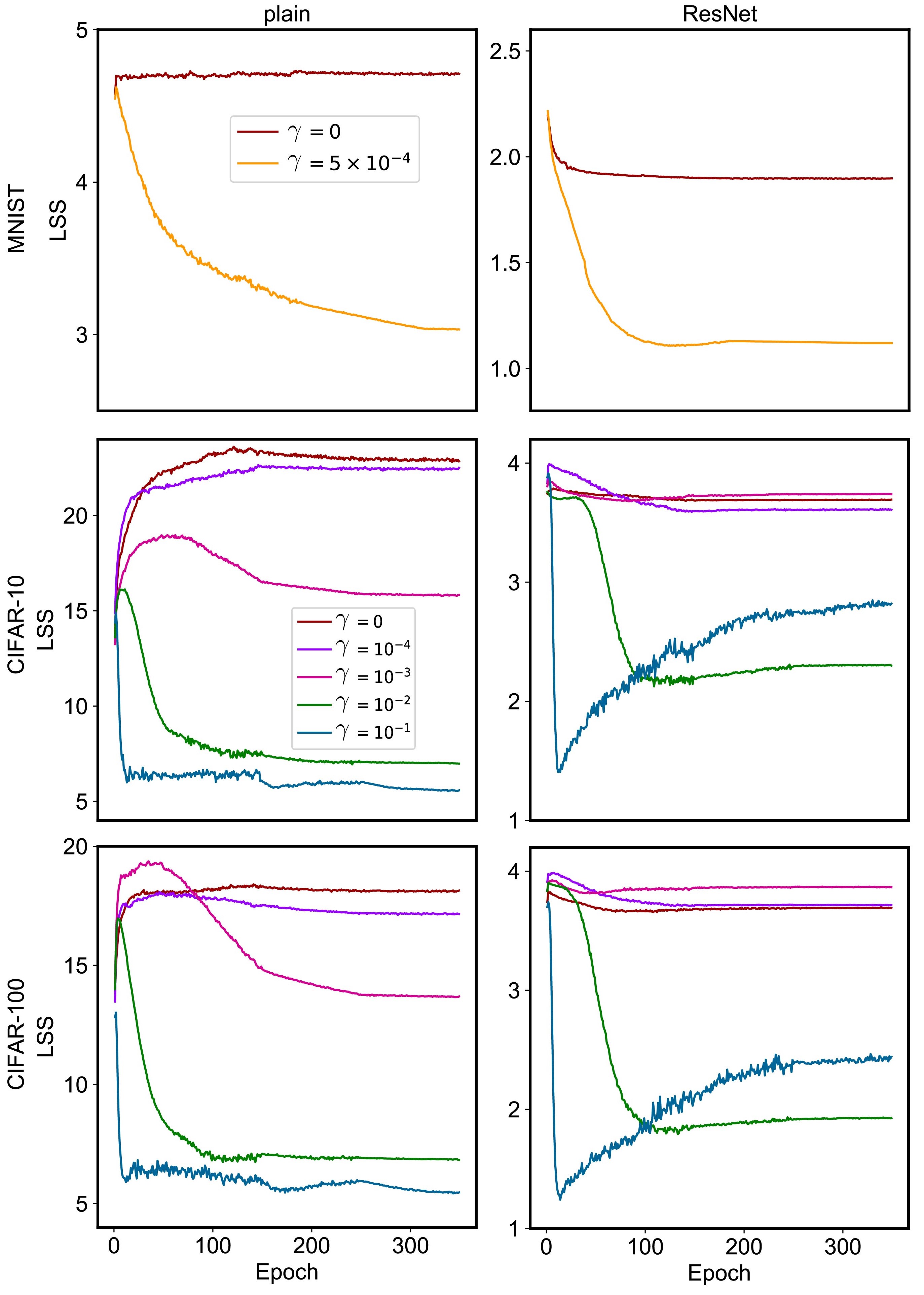
Figure 2: Performance comparison between plain networks and ResNets in terms of LSS with different $\gamma$s in the training process on MNIST, CIFAR-10 and CIFAR-100.

Figure 3: Two-dimensional visualization of data tracks with five segments for both plain networks and ResNets on MNIST. The original data representations of 1000 dimension are projected into two-dimensional space by multiplying them with a $2\times 1000$ random Gaussian matrix.

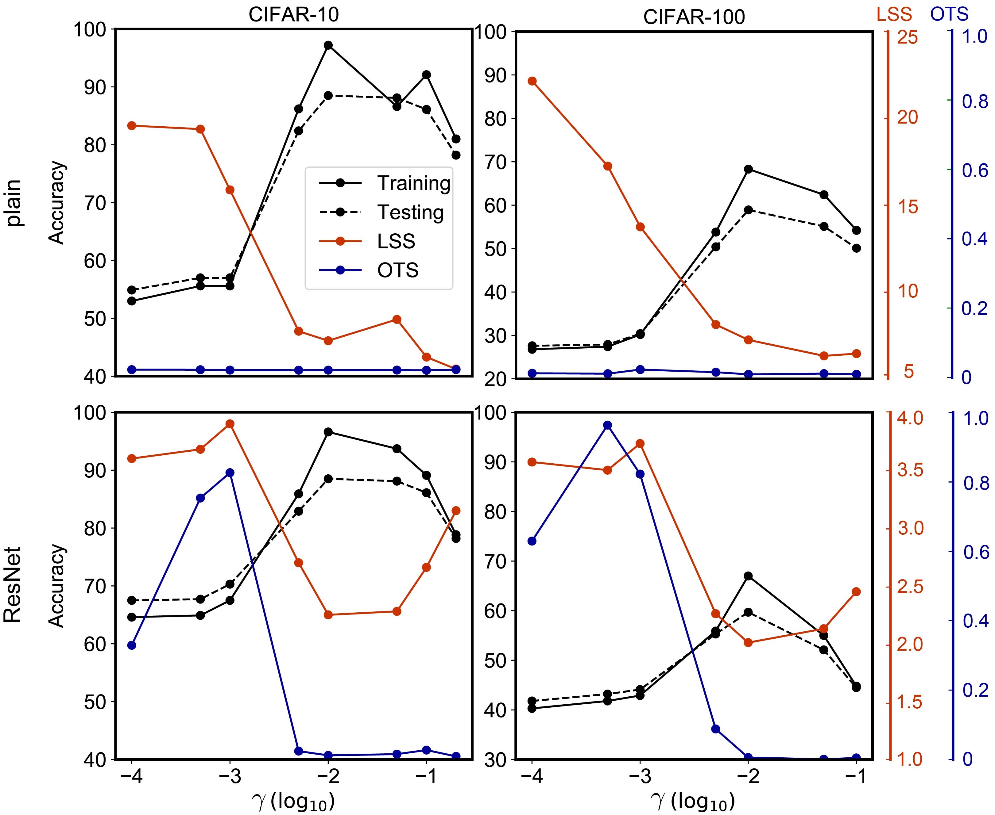
Figure 4: Comparison of change trend of training accuracy, testing accuracy, LSS and OTS in terms of $\gamma$s for plain networks and ResNets with $K=1$ on CIFAR-10 and CIFAR-100 respectively.

5.2 DNN indeed tends to approximate the geodesic curve

Numerical experiments show that the weight decay in both plain network and ResNet plays a role to force the tracks to approximate straight lines in their training process (Fig. 2). We can clearly see that LSS approaches to 1 when $\gamma$ is moderately large. For MNIST, both plain network and ResNet could achieve very small LSS even with a relatively small $\gamma$ (Fig. 2). While ResNet indeed results in line-shape data tracks ($\operatorname{LSS}=1.12$) and matches well with the optimal transport map ($\operatorname{OTS}=0.96$) with $\gamma=5\times 10^{-4}$, suggesting it could well approximate the geodesic curve in the Wasserstein space (Fig. 3). We note that the digital images of MNIST in the same class are relatively similar, which leads to many of the equations $y_{i}=f(x_{i})$ to be solved are degenerate. Thus, the tracks are more easily to be forced to straight lines by the weight decay. For CIFAR-10 and CIFAR-100, both plain network and ResNet need relatively large $\gamma$ to decrease LSS, and finally reached about 6.1 and 2.2 respectively (Fig. 2). This is because these two classification problems are more difficult to solve due to the redundant information among these data, which blocks the linearization of data tracks.

5.3 Better line shape of data tracks leads to higher accuracy

We observe that the training and testing accuracy both increase when the LSS decreases dramatically with $\gamma\in[10^{-3},10^{-2}]$ on both CIFAR-10 and CIFAR-100 respectively (Fig. 4). This illustrates that, when the data tracks are closer to straight lines, both networks have more power to fit the training data, which strongly supports our theoretical derivation about optimization. Meanwhile, the OTS of ResNet almost decreases to 0. If the input distribution and output one are fixed, then the optimal transport map $T$ is fixed which may not fit the data labels well. According to polar factorization theorem (Section 2), when $f$ fits the label better, the component of $\phi$ in the polar factorization is larger. This illustrates why the OTS of ResNet decreases dramatically with the increase of training accuracy. The testing accuracy increases with training accuracy because ResNet is more layerwise robust with larger $\gamma$ according to Section 4.1. When $\gamma$ is larger than 0.1, the weight decay tends to block the fitting process and then both training and testing accuracy decrease.

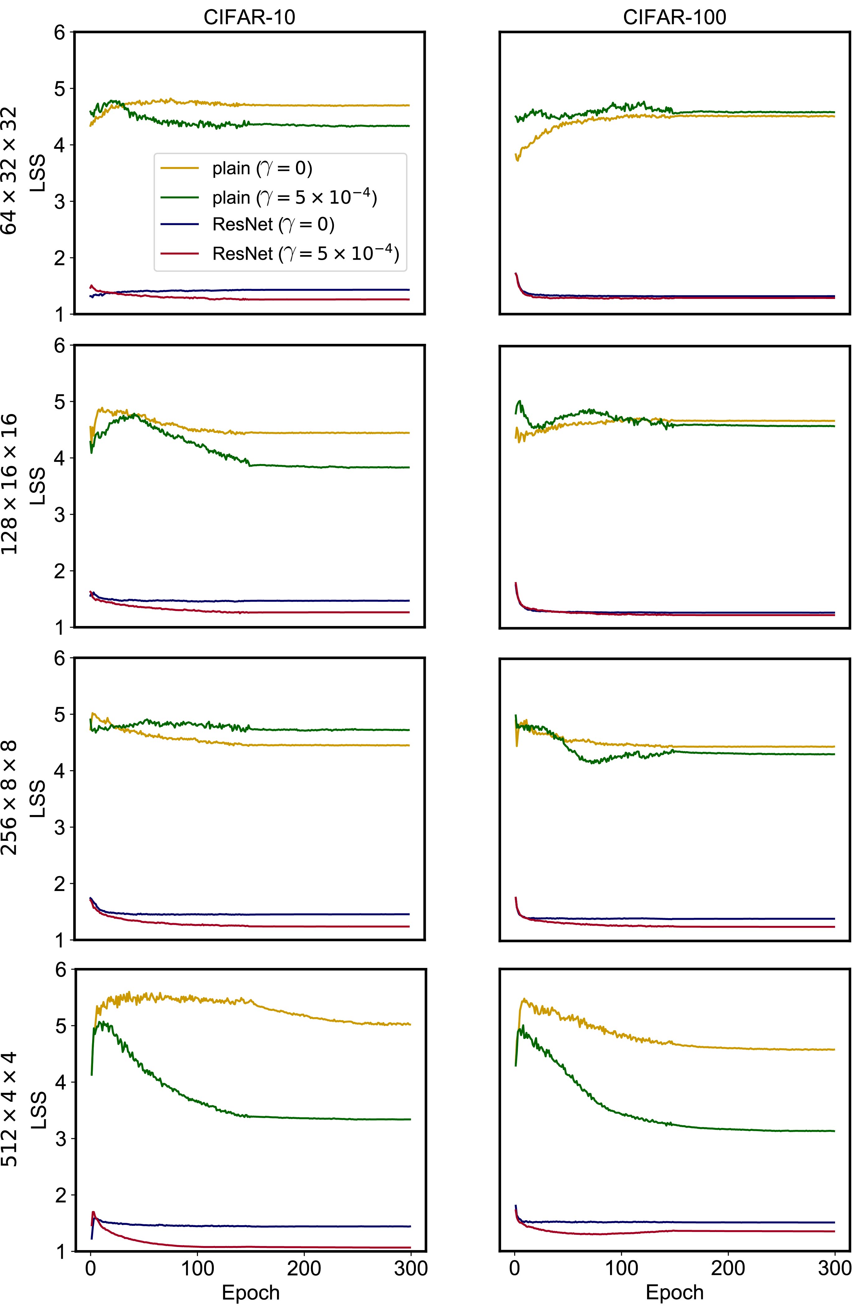
Figure 5: Performance comparison between plain networks and ResNets in terms of LSS for four diverse dimensions (i.e., $K=4$) on CIFAR-10 and CIFAR-100 respectively. The dimensions of four blocks are $64\times 32\times 32$, $128\times 16\times 16$, $256\times 8\times 8$, $512\times 4\times 4$ from top to bottom respectively.

5.4 ResNet approximates the geodesic curve better than plain network

While reducing the dimensions with $K=4$, the information irrelevant to the label can be dropped. Thus, the classification problem becomes relatively easy to solve and the training accuracy of ResNets and plain networks is close to $100\%$ on both CIFAR-10 and CIFAR-100 respectively. Both plain network and ResNet with $K=4$ can get smaller LSS compared to that with $K=1$, and approach about 4 and 1.2 for each dimension respectively (Fig. 5). Though the performance of ResNets and plain networks is similar on training data, ResNets has superiority in generalization with respect to testing accuracy over plain networks. We can clearly see that the OTS and LSS of ResNets are closer to 1 (Fig. 6), which suggests that ResNet approximates the geodesic curve better than plain network. On the contrary, the tracks of plain networks zigzag with high LSS and are arranged with OTS closing to 0. This illustrates why ResNets generalizes better in practice. We also confirm the derivations that ResNet is not dominated by individual units and more robust to both random and adversarial noises (see Appendix). The variance of scores on different dimensions in both ResNets and plain networks is large. This is due to the imbalance of number of parameters on different dimensions. For instance, the $64\times 32\times 32$ tensor is 8 times dimension of $512\times 4\times 4$ tensor, however, while utilizing $3\times 3$ convolution kernels, the number of parameters ($512\times 512\times 3\times 3$) in each layer on the latter is 64 times that of the former ($64\times 64\times 3\times 3$). Therefore, the tracks on the $512\times 4\times 4$ dimension are more flexible to be linearized than that on $64\times 32\times 32$ dimension. We can conjecture that the performance of DNN can be influenced by this kind of imbalance which may increase with $\gamma$. As a consequence of that, on the dimension-varying situation $K=4$, the best testing accuracy of ResNet and plain network are achieved when $\gamma=5\times 10^{-3}$ and $\gamma=1\times 10^{-3}$ respectively, while it is achieved with $\gamma=1\times 10^{-2}$ for $K=1$.

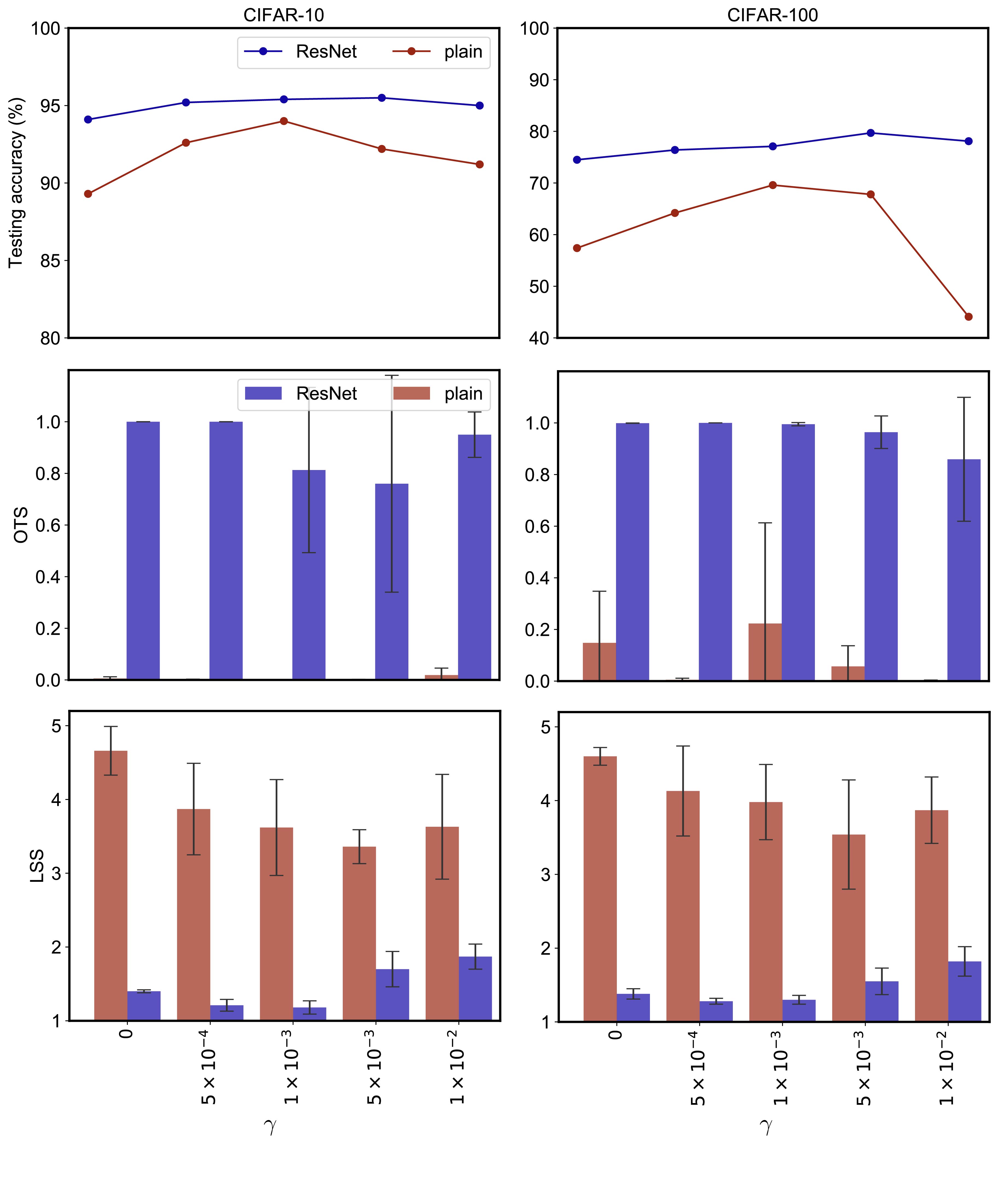
Figure 6: Performance comparison of plain networks and ResNets in terms of testing accuracy, OTS, LSS for four diverse dimensions (i.e., $K=4$) on CIFAR-10 and CIFAR-100 respectively. Four hyper-parameter $\gamma$s are used for evaluation.

6 Conclusion and discussion

Deep learning is a rising technique that has many important applications. However, the mathematical understanding of deep learning is still in its early stage. Moreover, deep learning is easy to attack and theoretical understanding could help us to overcome this weakness and design more powerful and robust models.

We build the connection of DNN and the geodesic curve in the Wasserstein space, which provides insights into the black box internal of DNN. Though ResNet approximates the geodesic curve better than plain network, it may not be a perfect implement in high-dimensional space due to its layerwise heterogeneity. How to design a better DNN in the spirit of the geodesic curve is an open problem which is worth to be explored in future.

The problem of optimal transport stems from Monge [35]. For the problem on a plane, Monge obtained the solution by means of very simple consideration that the routes of two elements must not cross each other. For DNN, if two data tracks intersect or close to intersect, then they can be easily mixed up by adding a noise, which provides us an intuition to interpret DNN. Nowadays, optimal transport has been developed to a mature branch of mathematics and has found its usage in solving tasks of deep learning such as image generation [4] and domain adaption [16]. In this paper, we interpret DNN as an approximation to geodesic curve in the Wasserstein space, which is a new aspect on building the internal connection of deep learning and optimal transport.

On the contrary, DNN could help to solve optimal transport problem. DNN is becoming a powerful tool to solve highly nonlinear or high-dimensional problems in scientific computation, such as solving high dimensional PDEs [27][39] and molecular dynamics [11][8][48]. However, there are still challenges to solve optimal transport problem under high-dimension, big data or continuous distribution. For the computation of optimal transport, several studies attempted to reduce computational complexity or enhance accuracy [17][18][22]. In short, we believe that DNN can serve as a powerful tool to solve these problems and find its usage in the future.

Acknowledgments

This work has been supported by the National Key Research and Development Program of China [2019YFA0709501]; National Natural Science Foundation of China [61621003]; National Ten Thousand Talent Program for Young Top-notch Talents; CAS Frontier Science Research Key Project for Top Young Scientist [QYZDB-SSW-SYS008].

7 Appendix

7.1 ResNet is not dominated by individual units

Some studies [50][10][9] revealed that each individual unit of DNN has different semantics and matches a diverse set of object concepts. As we discussed, the data tracks of plain network zigzag to change their directions frequently, and data representations of ResNet are forward propagated through line-shape tracks approximately. Thus, for ResNet, each layer contributes a part to the final transportation without changing the direction of tracks significantly.

To test the contribution of individual units in the $l$-th layer, we first obtain the most important units corresponding to each class by the average of all the data points in the class. Then for each $x$, we set the important units of $x^{(l)}$ to the same as that of $x^{(l-1)}$ to eliminate the effect of the $l$-th layer. Experiments show that for ResNet the testing accuracy doesn’t change significantly, while the testing accuracy of plain network falls rapidly with the increasing number of eliminated units (Fig. 7). This observation confirms our theoretical derivation that ResNet is not dominated by individual units, since it approximates the geodesic curve in the Wasserstein space.

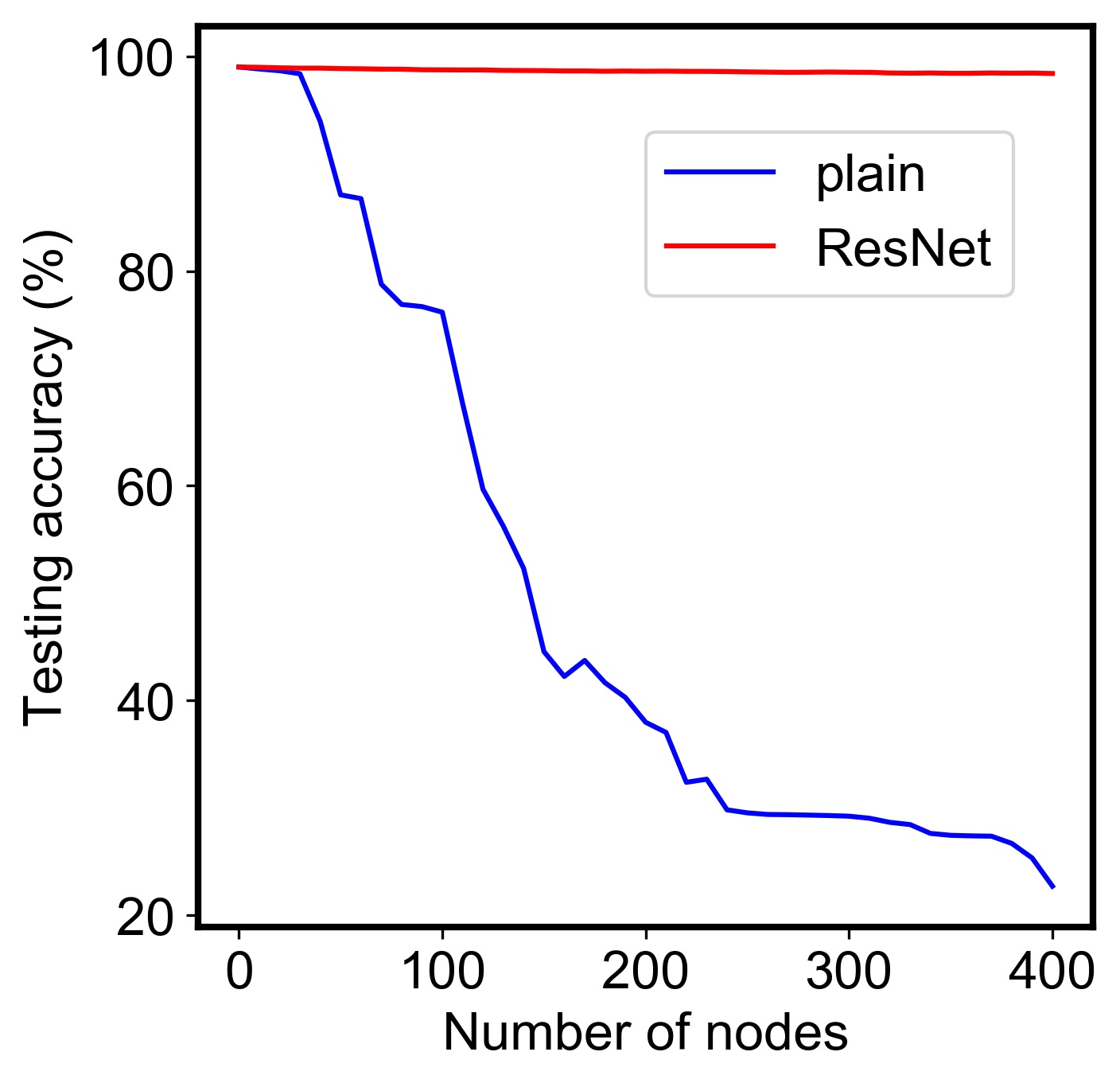
Figure 7: Testing accuracy of the five-block ResNet and corresponding plain network with the eliminated units in 3rd layer on MNIST.

7.2 ResNet is robust to both random and adversarial noises

According to the theoretical analysis in Section 4, ResNet is more robust to noise since it can better approximate the geodesic curve in the Wasserstein space. To test this, we train a ResNet and a plain network with $K=4$ on CIFAR-100. After training, the summation of loss over all the training data of the ResNet and plain network is 2.075 and 1.773 respectively. However, experiments show that ResNet is much robust to both random noise and adversarial noise that the accuracy for classification fall slower than plain network with the increase of noise (Fig. 8).

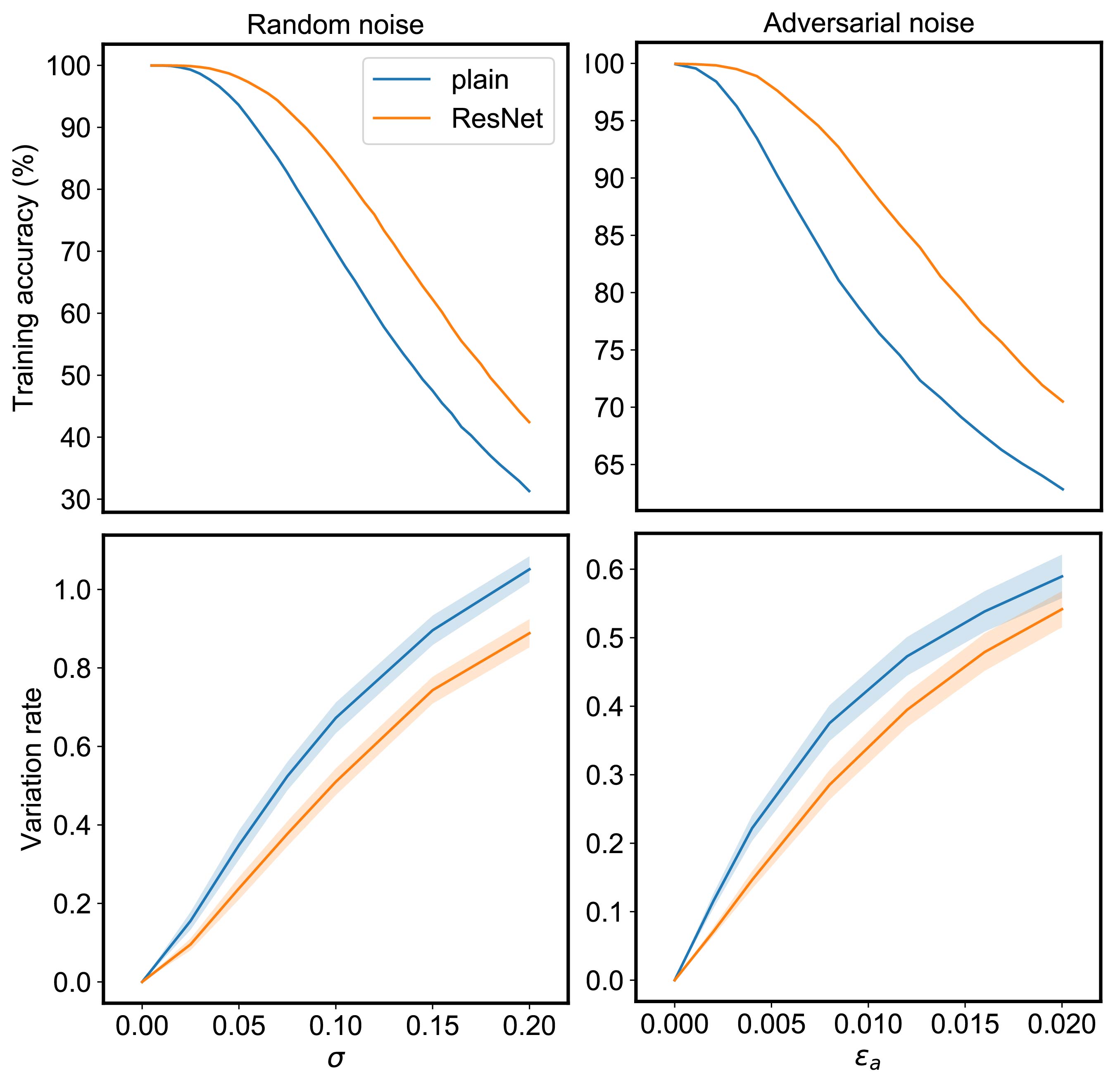
Figure 8: Comparison of plain network and ResNet on the data with random noise (left) and adversarial noise (right).

For each data point $x$ in the dataset $\mathcal{D}$, the data with random noise can be denoted by $x_{r}=x+e_{r}$, where $e_{r}\sim\mathcal{N}(0_{d\times 1},\sigma)$. The data with adversarial noise is constructed by the fast gradient sign method (FGSM) [23], i.e., $x_{a}=x+\epsilon_{a}\operatorname{sign}\left(\frac{\partial\mathcal{L}}{\partial x}\right)$, where $\epsilon_{a}$ is the coefficient of the noise and sign indicates the positive or negative symbol. Then the variation rate in the $l$-th layer by adding random or adversarial noise to the original data $\operatorname{Vr}_{r}(l,\sigma)$ and $\operatorname{Vr}_{a}(l,\sigma)$ can be defined by

$$\operatorname{Vr}_{r}(l,\sigma)=\sum_{x\in\mathcal{D}}\frac{\|x^{(l)}-x^{(l)}_{r}\|_{2}}{\|x^{(l)}\|_{2}|\mathcal{D}|},\quad\operatorname{Vr}_{a}(l,\sigma)=\sum_{x\in\mathcal{D}}\frac{\|x^{(l)}-x^{(l)}_{a}\|_{2}}{\|x^{(l)}\|_{2}|\mathcal{D}|}.$$ (49)

As we can see, the variation rate curve of the ResNet when $l=n$ is lower than that of the plain network (Fig. 8), indicating that ResNet could decrease the probability for the noisy data to be mis-classified.

7.3 Proportion of segment lengths of data tracks of DNNs on CIFAR-100

We show the proportion of segment lengths of data tracks of plain networks and ResNets on CIFAR-100 with $K=4$ on CIFAR-100 respectively (Tables 2-3).

Table 2: Proportion of segment lengths of data tracks in plain networks on CIFAR-100.

$\gamma$	$S_{1}$	$S_{2}$	$S_{3}$	$S_{4}$	$S_{5}$	$S_{6}$	$S_{7}$	$S_{8}$	$S_{9}$	$S_{10}$
0	0.076	0.103	0.093	0.104	0.106	0.102	0.105	0.107	0.117	0.087
$1\times 10^{-4}$	0.079	0.097	0.103	0.097	0.103	0.103	0.107	0.112	0.115	0.083
$5\times 10^{-4}$	0.072	0.102	0.103	0.106	0.101	0.114	0.099	0.119	0.099	0.086
$1\times 10^{-3}$	0.076	0.105	0.099	0.109	0.098	0.092	0.094	0.102	0.112	0.107
$5\times 10^{-3}$	0.035	0.039	0.042	0.041	0.039	0.042	0.039	0.038	0.036	0.643
$1\times 10^{-2}$	0.019	0.012	0.013	0.013	0.013	0.012	0.012	0.011	0.010	0.880
$5\times 10^{-2}$	0.010	0.003	0.003	0.003	0.003	0.002	0.002	0.001	0.001	0.969
$1\times 10^{-1}$	8.97$\times 10^{-3}$	2.95$\times 10^{-3}$	2.85$\times 10^{-3}$	2.55$\times 10^{-3}$	1.78$\times 10^{-3}$	1.40$\times 10^{-3}$	1.05$\times 10^{-3}$	6.92$\times 10^{-4}$	8.77$\times 10^{-4}$	0.977
$5\times 10^{-1}$	0.118	0.130	0.109	0.093	0.088	0.103	0.091	0.087	0.080	0.095

Table 3: Proportion of segment lengths of data tracks in ResNets on CIFAR-100.

$\gamma$	$S_{1}$	$S_{2}$	$S_{3}$	$S_{4}$	$S_{5}$	$S_{6}$	$S_{7}$	$S_{8}$	$S_{9}$	$S_{10}$
0	0.264	0.121	0.088	0.087	0.085	0.074	0.067	0.059	0.082	0.068
$1\times 10^{-4}$	0.218	0.126	0.091	0.083	0.076	0.075	0.082	0.071	0.091	0.084
$5\times 10^{-4}$	0.238	0.111	0.109	0.074	0.066	0.091	0.075	0.088	0.068	0.075
$1\times 10^{-3}$	0.247	0.111	0.092	0.090	0.069	0.084	0.060	0.070	0.091	0.082
$5\times 10^{-3}$	0.067	0.059	0.074	0.068	0.087	0.092	0.084	0.135	0.147	0.183
$1\times 10^{-2}$	0.009	0.007	0.009	0.010	0.029	0.079	0.204	0.184	0.242	0.223
$5\times 10^{-2}$	0.002	0.002	0.002	0.003	0.009	0.171	0.219	0.182	0.239	0.168
$1\times 10^{-1}$	0.001	0.001	0.001	0.002	0.002	0.003	0.012	0.203	0.054	0.721
$5\times 10^{-1}$	0.145	0.097	0.090	0.102	0.097	0.085	0.099	0.093	0.111	0.078

7.4 Visualization of data tracks of DNNs

We show the visualization of data tracks of plain networks and ResNets with $K=1$ and $K=4$ on both CIFAR-10 and on CIFAR-100 respectively (Figures 9-16).

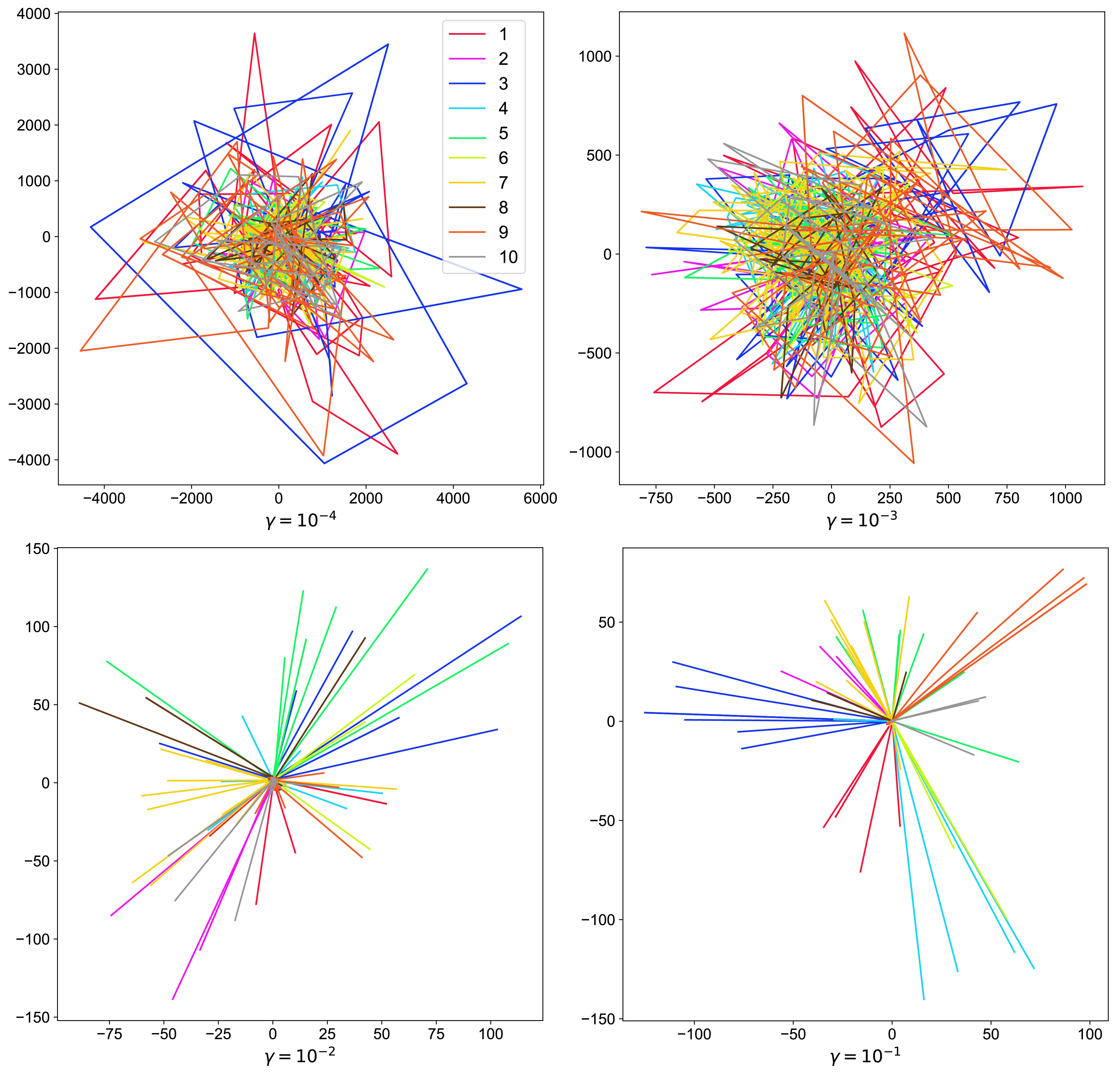
Figure 9: Visualization of data tracks of plain networks when $K=1$ with $\gamma=10^{-4}$, $\gamma=10^{-3}$, $\gamma=10^{-2}$, $\gamma=10^{-1}$ on CIFAR-10.

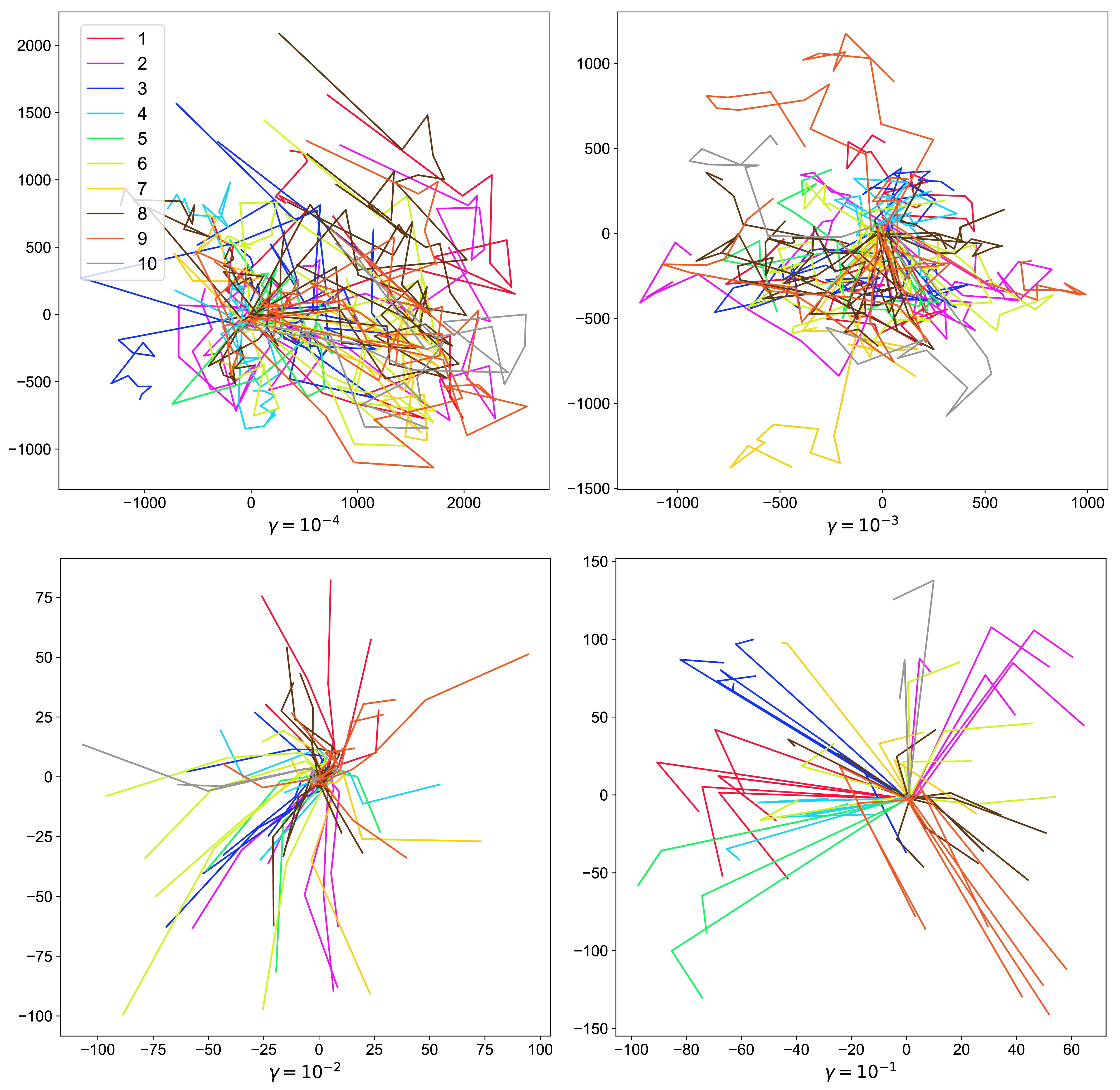
Figure 10: Visualization of data tracks of ResNets when $K=1$ with $\gamma=10^{-4}$, $\gamma=10^{-3}$, $\gamma=10^{-2}$, $\gamma=10^{-1}$ on CIFAR-10.

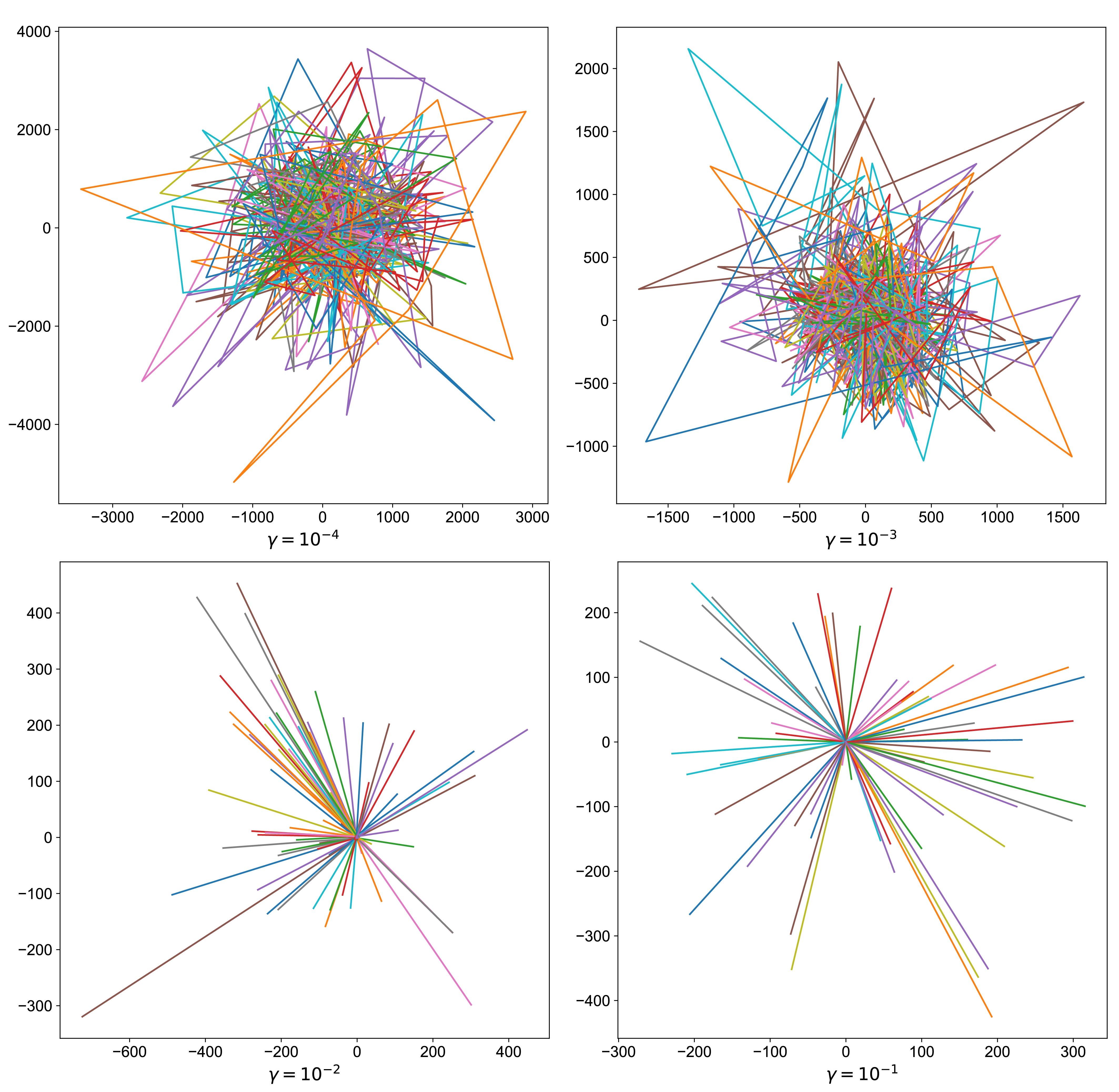
Figure 11: Visualization of data tracks of plain networks when $K=1$ with $\gamma=10^{-4}$, $\gamma=10^{-3}$, $\gamma=10^{-2}$, $\gamma=10^{-1}$ on CIFAR-100.

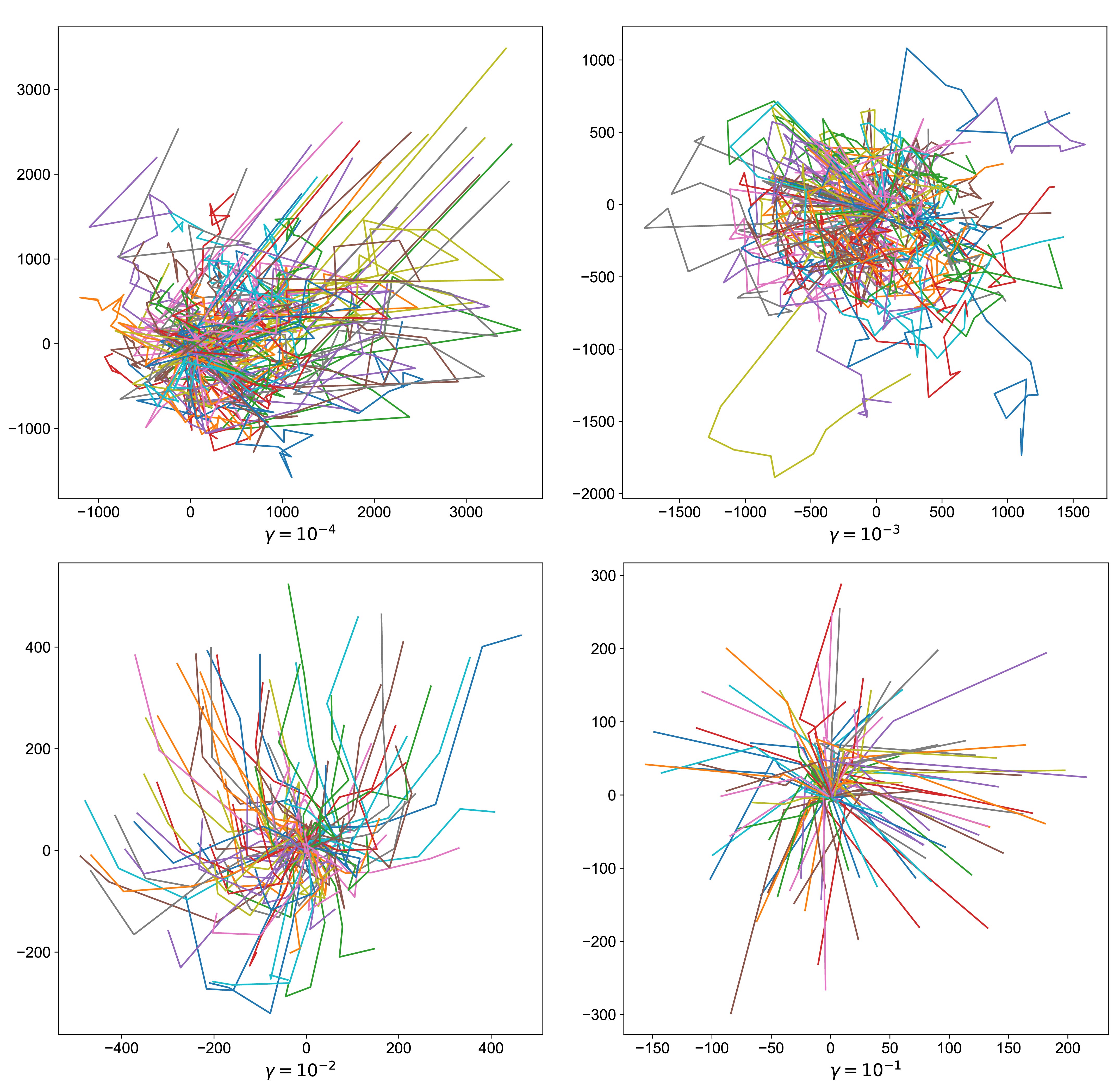
Figure 12: Visualization of data tracks of ResNets when $K=1$ with $\gamma=10^{-4}$, $\gamma=10^{-3}$, $\gamma=10^{-2}$, $\gamma=10^{-1}$ on CIFAR-100.

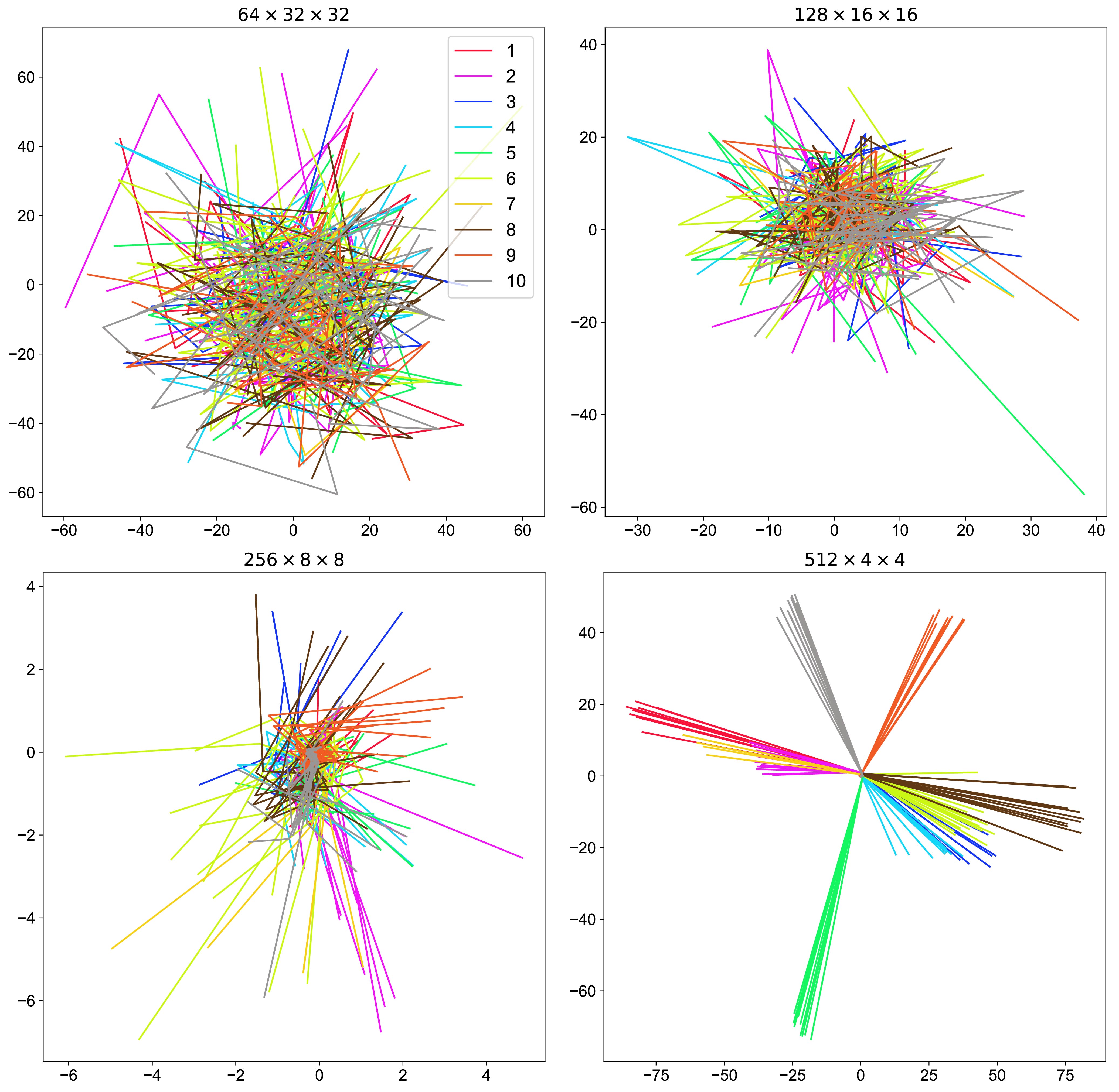
Figure 13: Visualization of data tracks of plain networks when $K=4$ with $\gamma=10^{-3}$ on CIFAR-10.

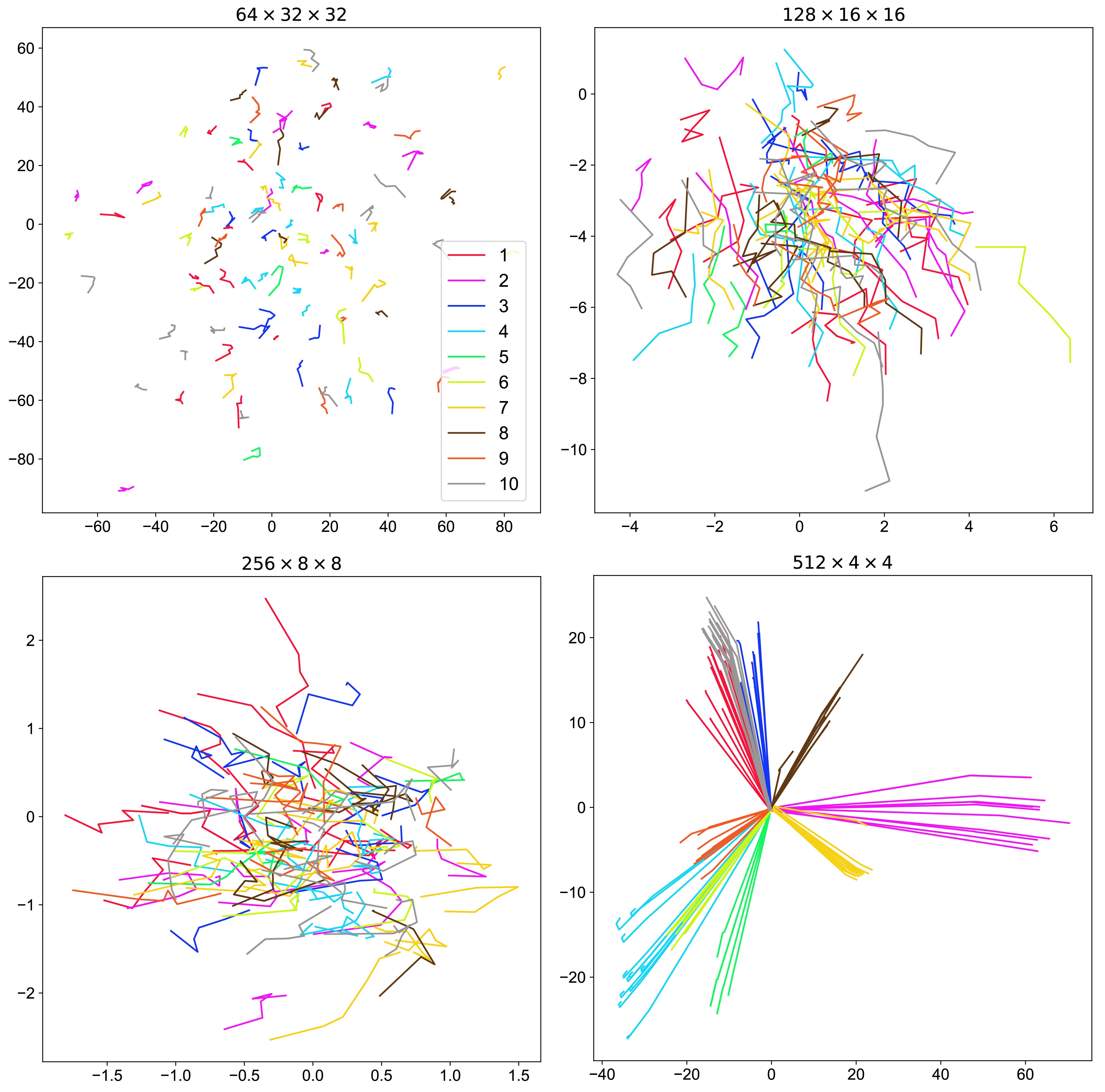
Figure 14: Visualization of data tracks of ResNets when $K=4$ with $\gamma=5\times 10^{-3}$ on CIFAR-10.

Figure 15: Visualization of data tracks of plain networks when $K=4$ with $\gamma=10^{-3}$ on CIFAR-100.

Figure 16: Visualization of data tracks of ResNets when $K=4$ with $\gamma=5\times 10^{-3}$ on CIFAR-100.

7.5 Performance comparison of DNNs

We show the performance comparison of plain networks and ResNets with $K=1$ and $K=4$ in terms of testing accuracy, OTS, LSR and LSS on both CIFAR-10 and CIFAR-100 respectively (Tables 4-7).

Table 4: Performance comparison of plain networks and ResNets with $K=1$ in terms of testing accuracy, OTS, LSR and LSS on the CIFAR-10.

$\gamma$	Training Accuracy ($\%$)		Testing Accuracy ($\%$)		OTS		LSR		LSS
	plain	ResNet	plain	ResNet	plain	ResNet	plain	ResNet	plain	ResNet
0	52.1	63.0	53.5	66.3	$9.0\times 10^{-4}$	0.681	78.5	3.71	20.2	3.79
$1\times 10^{-4}$	53.0	64.6	54.9	67.5	$2.3\times 10^{-3}$	0.329	67.9	3.30	19.1	3.60
$5\times 10^{-4}$	55.6	64.9	57.0	67.7	$2.1\times 10^{-3}$	0.753	51.2	3.57	18.9	3.68
$1\times 10^{-3}$	55.6	67.5	57.0	70.3	$1.0\times 10^{-3}$	0.826	28.8	3.81	15.4	3.90
$5\times 10^{-3}$	86.2	85.9	82.4	82.9	$8.0\times 10^{-4}$	0.0242	2.26	2.07	7.26	2.70
$1\times 10^{-2}$	97.2	96.6	88.9	88.5	$9.0\times 10^{-4}$	0.0119	1.27	1.24	6.71	2.25
$5\times 10^{-2}$	86.6	93.7	81.9	88.1	$1.1\times 10^{-3}$	0.0155	1.07	1.19	7.94	2.28
$1\times 10^{-1}$	92.1	89.1	88.0	86.1	$5.0\times 10^{-4}$	0.0272	1.04	1.22	5.77	2.66
$2\times 10^{-2}$	81.0	78.8	79.0	78.2	$2.4\times 10^{-3}$	0.009	1.04	1.17	5.08	3.15

Table 5: Performance comparison of plain networks and ResNets with $K=1$ in terms of training and testing accuracy, OTS, LSR and LSS on CIFAR-100.

$\gamma$	Training Accuracy ($\%$)		Testing Accuracy ($\%$)		OTS		LSR		LSS
	plain	ResNet	plain	ResNet	plain	ResNet	plain	ResNet	plain	ResNet
0	27.3	40.3	27.3	42.4	$5.3\times 10^{-3}$	0.205	48.6	3.62	20.1	3.47
$1\times 10^{-4}$	26.8	40.3	27.6	41.8	$3.4\times 10^{-3}$	0.629	43.9	3.57	21.9	3.57
$5\times 10^{-4}$	27.4	41.8	27.9	43.2	$2.2\times 10^{-3}$	0.963	30.8	3.48	17.0	3.50
$1\times 10^{-3}$	30.2	42.9	30.4	44.1	$1.41\times 10^{-2}$	0.822	15.4	3.62	13.5	3.73
$5\times 10^{-3}$	53.8	55.9	50.4	55.3	$6.5\times 10^{-3}$	0.088	1.55	2.17	7.87	2.26
$1\times 10^{-2}$	68.3	67.0	58.9	59.7	$3\times 10^{-4}$	$5.70\times 10^{-3}$	1.13	1.52	6.99	2.01
$5\times 10^{-2}$	62.4	55.0	55.1	52.1	$2.4\times 10^{-3}$	$7\times 10^{-4}$	1.03	1.51	6.07	2.13
$1\times 10^{-1}$	54.2	44.8	50.1	44.5	$5\times 10^{-4}$	$4.6\times 10^{-3}$	1.02	1.14	6.20	2.45
$2\times 10^{-2}$	12.6	14.0	11.8	12.0	$2.2\times 10^{-3}$	$2.3\times 10^{-3}$	1.02	1.29	5.85	3.37

Table 6: Performance comparison of plain networks and ResNets with $K=4$ in terms of testing accuracy, OTS, LSR and LSS on CIFAR-10.

$\gamma$	Testing Accuracy ($\%$)		OTS (std)		LSR (std)		LSS (std)
	plain	ResNet	plain	ResNet	plain	ResNet	plain	ResNet
0	89.3	94.1	$5.5\times 10^{-3}$ ($6.7\times 10^{-3}$)	1 (0)	3.40 (0.27)	1.30 (0.022)	4.66 (0.33)	1.40 (0.02)
$5\times 10^{-4}$	92.6	95.2	$1.75\times 10^{-3}$ ($1.3\times 10^{-3}$)	1 (0)	3.33 (0.94)	1.17 (0.071)	3.87 (0.62)	1.21 (0.08)
$1\times 10^{-3}$	94.0	95.4	0 (0)	0.813 (0.32)	2.55 (0.97)	1.16 (0.080)	3.62 (0.65)	1.18 (0.09)
$5\times 10^{-3}$	92.2	95.5	$1.25\times 10^{-3}$ ($1.1\times 10^{-3}$)	0.760 (0.42)	2.13 (0.61)	1.49 (0.34)	3.36 (0.23)	1.70 (0.24)
$1\times 10^{-2}$	91.2	95.0	0.0188 (0.027)	0.950 (0.088)	1.88 (0.55)	1.56 (0.32)	3.63 (0.71)	1.87 (0.17)

Table 7: Performance comparison of plain networks and ResNets with $K=4$ in terms of testing accuracy, OTS, LSR and LSS on CIFAR-100.

$\gamma$	Testing Accuracy ($\%$)		OTS (std)		LSR (std)		LSS (std)
	plain	ResNet	plain	ResNet	plain	ResNet	plain	ResNet
0	57.4	74.5	0.148 (0.20)	0.999 ($6.0\times 10^{-4}$)	3.74 (0.37)	1.35 (0.09)	4.60 (0.12)	1.38 (0.07)
$5\times 10^{-4}$	64.2	76.4	0.005 (0.006)	1 (0)	3.56 (0.33)	1.20 (0.027)	4.13 (0.61)	1.28 (0.04)
$1\times 10^{-3}$	69.6	77.1	0.223 (0.39)	0.995 ($6.4\times 10^{-3}$)	3.08 (0.44)	1.21 (0.055)	3.98 (0.51)	1.30 (0.06)
$5\times 10^{-3}$	67.8	79.7	0.057 (0.08)	0.964 ($6.3\times 10^{-2}$)	2.79 (0.70)	1.43 (0.23)	3.54 (0.74)	1.55 (0.18)
$1\times 10^{-2}$	44.1	78.1	0.003 (0.001)	0.859 (0.24)	2.99 (1.18)	1.66 (0.36)	3.87 (0.45)	1.82 (0.20)

References

- Allen-Zhu et al. [2019a] Zeyuan Allen-Zhu, Yuanzhi Li, and Yingyu Liang. Learning and generalization in overparameterized neural networks, going beyond two layers. In Advances in Neural Information Processing Systems, pages 6158–6169, 2019a.
- Allen-Zhu et al. [2019b] Zeyuan Allen-Zhu, Yuanzhi Li, and Zhao Song. A convergence theory for deep learning via over-parameterization. In International Conference on Machine Learning, pages 242–252. PMLR, 2019b.
- Ambrosio and Gigli [2013] Luigi Ambrosio and Nicola Gigli. A user’s guide to optimal transport. In Modelling and optimisation of flows on networks, pages 1–155. Springer, 2013.
- Arjovsky et al. [2017] Martin Arjovsky, Soumith Chintala, and Léon Bottou. Wasserstein generative adversarial networks. In Proceedings of the 34th International Conference on Machine Learning, volume 70, pages 214–223, 2017.
- Arora et al. [2019a] Sanjeev Arora, Nadav Cohen, Wei Hu, and Yuping Luo. Implicit regularization in deep matrix factorization. In Advances in Neural Information Processing Systems, pages 7413–7424, 2019a.
- Arora et al. [2019b] Sanjeev Arora, Simon S Du, Wei Hu, Zhiyuan Li, and Ruosong Wang. Fine-grained analysis of optimization and generalization for overparameterized two-layer neural networks. In International Conference on Machine Learning, pages 477–502. International Machine Learning Society (IMLS), 2019b.
- Arora et al. [2019c] Sanjeev Arora, Noah Golowich, Nadav Cohen, and Wei Hu. A convergence analysis of gradient descent for deep linear neural networks. In International Conference on Learning Representations, pages 1–12, 2019c.
- Bartók et al. [2010] Albert P Bartók, Mike C Payne, Risi Kondor, and Gábor Csányi. Gaussian approximation potentials: the accuracy of quantum mechanics, without the electrons. Physical Review Letters, 104(13):136403, 2010.
- Bau et al. [2019] Anthony Bau, Yonatan Belinkov, Hassan Sajjad, Nadir Durrani, Fahim Dalvi, and James Glass. Identifying and controlling important neurons in neural machine translation. International Conference on Learning Representations, pages 1–13, 2019.
- Bau et al. [2020] David Bau, Jun-Yan Zhu, Hendrik Strobelt, Agata Lapedriza, Bolei Zhou, and Antonio Torralba. Understanding the role of individual units in a deep neural network. Proceedings of the National Academy of Sciences, 117(48):30071–30078, 2020.
- Behler and Parrinello [2007] Jörg Behler and Michele Parrinello. Generalized neural-network representation of high-dimensional potential-energy surfaces. Physical Review Letters, 98(14):146401, 2007.
- Benamou and Brenier [1999] Jean-David Benamou and Yann Brenier. A numerical method for the optimal time-continuous mass transport problem and related problems. Contemporary Mathematics, 226:1–12, 1999.
- Brenier [1991] Yann Brenier. Polar factorization and monotone rearrangement of vector-valued functions. Communications on Pure and Applied Mathematics, 44(4):375–417, 1991.
- Cao and Gu [2020] Yuan Cao and Quanquan Gu. Generalization error bounds of gradient descent for learning over-parameterized deep relu networks. In Proceedings of the AAAI Conference on Artificial Intelligence, volume 34, pages 3349–3356, 2020.
- Chang et al. [2018] Bo Chang, Lili Meng, Eldad Haber, Frederick Tung, and David Begert. Multi-level residual networks from dynamical systems view. International Conference on Learning Representations, pages 1–14, 2018.
- Courty et al. [2016] Nicolas Courty, Rémi Flamary, Devis Tuia, and Alain Rakotomamonjy. Optimal transport for domain adaptation. IEEE Transactions on Pattern Analysis and Machine Intelligence, 39(9):1853–1865, 2016.
- Cuturi [2013] Marco Cuturi. Sinkhorn distances: Lightspeed computation of optimal transport. In Advances in Neural Information Processing Systems, pages 2292–2300, 2013.
- Deshpande et al. [2018] Ishan Deshpande, Ziyu Zhang, and Alexander G Schwing. Generative modeling using the sliced wasserstein distance. In Proceedings of the IEEE Conference on Computer Vision and Pattern Recognition, pages 3483–3491, 2018.
- Du and Hu [2019] Simon Du and Wei Hu. Width provably matters in optimization for deep linear neural networks. In International Conference on Machine Learning, pages 1655–1664, 2019.
- Du et al. [2019] Simon Du, Jason Lee, Haochuan Li, Liwei Wang, and Xiyu Zhai. Gradient descent finds global minima of deep neural networks. In International Conference on Machine Learning, pages 1675–1685, 2019.
- Du et al. [2018] Simon S Du, Xiyu Zhai, Barnabas Poczos, and Aarti Singh. Gradient descent provably optimizes over-parameterized neural networks. International Conference on Learning Representations, pages 1–13, 2018.
- Gai and Zhang [2020] Kuo Gai and Shihua Zhang. Tessellated wasserstein auto-encoders. arXiv preprint arXiv:2005.09923, 2020.
- Goodfellow et al. [2014] Ian J Goodfellow, Jonathon Shlens, and Christian Szegedy. Explaining and harnessing adversarial examples. International Conference on Learning Representations, pages 1–11, 2014.
- Greff et al. [2017] Klaus Greff, Rupesh K Srivastava, and Jürgen Schmidhuber. Highway and residual networks learn unrolled iterative estimation. International Conference on Learning Representations, pages 1–14, 2017.
- Guo and Zhang [2019] Zhenxing Guo and Shihua Zhang. Sparse deep nonnegative matrix factorization. Big Data Mining and Analytics, 3(1):13–28, 2019.
- Haber and Ruthotto [2017] Eldad Haber and Lars Ruthotto. Stable architectures for deep neural networks. Inverse Problems, 34(1):014004, 2017.
- Han et al. [2018] Jiequn Han, Arnulf Jentzen, and E Weinan. Solving high-dimensional partial differential equations using deep learning. Proceedings of the National Academy of Sciences, 115(34):8505–8510, 2018.
- He et al. [2016a] Kaiming He, Xiangyu Zhang, Shaoqing Ren, and Jian Sun. Deep residual learning for image recognition. In Proceedings of the IEEE Conference on Computer Vision and Pattern Recognition, pages 770–778, 2016a.
- He et al. [2016b] Kaiming He, Xiangyu Zhang, Shaoqing Ren, and Jian Sun. Identity mappings in deep residual networks. In European Conference on Computer Vision, pages 630–645. Springer, 2016b.
- Jacot et al. [2018] Arthur Jacot, Franck Gabriel, and Clément Hongler. Neural tangent kernel: convergence and generalization in neural networks. In Advances in Neural Information Processing Systems, pages 8571–8580, 2018.
- Jastrzebski et al. [2018] Stanisław Jastrzebski, Devansh Arpit, Nicolas Ballas, Vikas Verma, Tong Che, and Yoshua Bengio. Residual connections encourage iterative inference. In International Conference on Learning Representations, pages 1–14, 2018.
- Jonker and Volgenant [1987] Roy Jonker and Anton Volgenant. A shortest augmenting path algorithm for dense and sparse linear assignment problems. Computing, 38(4):325–340, 1987.
- Laurent and Brecht [2018] Thomas Laurent and James Brecht. Deep linear networks with arbitrary loss: All local minima are global. In International Conference on Machine Learning, pages 2902–2907. PMLR, 2018.
- Li and Liang [2018] Yuanzhi Li and Yingyu Liang. Learning overparameterized neural networks via stochastic gradient descent on structured data. In Advances in Neural Information Processing Systems, pages 8157–8166, 2018.
- Monge [1781] Gaspard Monge. Mémoire sur la théorie des déblais et des remblais. Histoire de l’Académie Royale des Sciences de Paris, 1781.
- Papyan et al. [2017] Vardan Papyan, Yaniv Romano, and Michael Elad. Convolutional neural networks analyzed via convolutional sparse coding. The Journal of Machine Learning Research, 18(1):2887–2938, 2017.
- Saxe et al. [2013] Andrew M Saxe, James L McClelland, and Surya Ganguli. Exact solutions to the nonlinear dynamics of learning in deep linear neural networks. arXiv preprint arXiv:1312.6120, 2013.
- Shamir [2019] Ohad Shamir. Exponential convergence time of gradient descent for one-dimensional deep linear neural networks. In Conference on Learning Theory, pages 2691–2713. PMLR, 2019.
- Sirignano and Spiliopoulos [2018] Justin Sirignano and Konstantinos Spiliopoulos. Dgm: A deep learning algorithm for solving partial differential equations. Journal of Computational Physics, 375:1339–1364, 2018.
- Trigeorgis et al. [2016] George Trigeorgis, Konstantinos Bousmalis, Stefanos Zafeiriou, and Björn W Schuller. A deep matrix factorization method for learning attribute representations. IEEE Transactions on Pattern Analysis and Machine Intelligence, 39(3):417–429, 2016.
- Veit et al. [2016] Andreas Veit, Michael J Wilber, and Serge Belongie. Residual networks behave like ensembles of relatively shallow networks. In Advances in Neural Information Processing Systems, pages 550–558, 2016.
- Wang et al. [2019] Bao Wang, Zuoqiang Shi, and Stanley Osher. Resnets ensemble via the feynman-kac formalism to improve natural and robust accuracies. In Advances in Neural Information Processing Systems, pages 1657–1667, 2019.
- Weinan [2017] E Weinan. A proposal on machine learning via dynamical systems. Communications in Mathematics and Statistics, 5(1):1–11, 2017.
- Xie et al. [2017] Saining Xie, Ross Girshick, Piotr Dollár, Zhuowen Tu, and Kaiming He. Aggregated residual transformations for deep neural networks. In Proceedings of the IEEE Conference on Computer Vision and Pattern Recognition, pages 1492–1500, 2017.
- Xu and Mannor [2012] Huan Xu and Shie Mannor. Robustness and generalization. Machine learning, 86(3):391–423, 2012.
- Xue et al. [2017] Hong-Jian Xue, Xinyu Dai, Jianbing Zhang, Shujian Huang, and Jiajun Chen. Deep matrix factorization models for recommender systems. In International Joint Conferences on Artificial Intelligence, volume 17, pages 3203–3209, 2017.
- Zagoruyko and Komodakis [2016] Sergey Zagoruyko and Nikos Komodakis. Wide residual networks. In Proceedings of the British Machine Vision Conference (BMVC), pages 87.1–87.12, 2016.
- Zhang et al. [2018] Linfeng Zhang, Jiequn Han, Han Wang, Roberto Car, and E Weinan. Deep potential molecular dynamics: a scalable model with the accuracy of quantum mechanics. Physical Review Letters, 120(14):143001, 2018.
- Zhang and Zhang [2020] Zhiyang Zhang and Shihua Zhang. Towards understanding residual and dilated dense neural networks via convolutional sparse coding. National Science Review, pages 1–13, 2020.
- Zhou et al. [2018] Bolei Zhou, Yiyou Sun, David Bau, and Antonio Torralba. Revisiting the importance of individual units in cnns via ablation. arXiv preprint arXiv:1806.02891, 2018.
- Zou et al. [2020] Difan Zou, Yuan Cao, Dongruo Zhou, and Quanquan Gu. Gradient descent optimizes over-parameterized deep relu networks. Machine Learning, 109(3):467–492, 2020.