\addtokomafont

title

Toy examples for effective concentration bounds

Benoît R. Kloeckner Université Paris-Est, Laboratoire d’Analyse et de Matématiques Appliquées (UMR 8050), UPEM, UPEC, CNRS, F-94010, Créteil, France
Abstract

In this note we prove a spectral gap for various Markov chains on various functional spaces. While proving that a spectral gap exists is relatively common, explicit estimates seems somewhat rare.

These estimates are then used to apply the concentration inequalities of [Klo17] (most of the present material was part of Section 3 of that article, which has been reduced to its core in the published version).

Let us recall briefly the notation and concentration inequalities from [Klo17].

Let (Xk)k0subscriptsubscript𝑋𝑘𝑘0(X_{k})_{k\geq 0} be a Markov chain taking value in a general state space ΩΩ\Omega with a unique stationary measure μ0subscript𝜇0\mu_{0}, and let φ:Ω:𝜑Ω\varphi:\Omega\to\mathbb{R} be a function (the “observable”). We are interested in the speed of the convergence of the empirical average μ^n(φ):=1nk=1nφ(Xk)assignsubscript^𝜇𝑛𝜑1𝑛superscriptsubscript𝑘1𝑛𝜑subscript𝑋𝑘\hat{\mu}_{n}(\varphi):=\frac{1}{n}\sum_{k=1}^{n}\varphi(X_{k}) to μ0(φ)subscript𝜇0𝜑\mu_{0}(\varphi). We denote by μ𝜇\mu the law of X0subscript𝑋0X_{0}, which can be arbitrary.

Assumption 1.

The observable φ𝜑\varphi belongs to a function space 𝒳𝒳\mathscr{X} satisfying

  1. i.

    its norm delimited-∥∥\lVert\cdot\rVert dominates the uniform norm: delimited-∥∥subscriptdelimited-∥∥\lVert\cdot\rVert\geq\lVert\cdot\rVert_{\infty},

  2. ii.

    𝒳𝒳\mathscr{X} is a Banach algebra, i.e. for all f,g𝒳𝑓𝑔𝒳f,g\in\mathscr{X} we have fgfgdelimited-∥∥𝑓𝑔delimited-∥∥𝑓delimited-∥∥𝑔\lVert fg\rVert\leq\lVert f\rVert\lVert g\rVert,

  3. iii.

    𝒳𝒳\mathscr{X} contains the constant functions and 𝟏=1delimited-∥∥11\lVert\boldsymbol{1}\rVert=1 (where 𝟏1\boldsymbol{1} denotes the constant function with value 111).

To the transition kernel 𝖬𝖬\mathsf{M} is associated an averaging operator acting on 𝒳𝒳\mathscr{X}:

L0f(x)=Ωf(y)dmx(y).subscriptL0𝑓𝑥subscriptΩ𝑓𝑦differential-dsubscript𝑚𝑥𝑦\mathrm{L}_{0}f(x)=\int_{\Omega}f(y)\mathrm{d}m_{x}(y).

Since each mxsubscript𝑚𝑥m_{x} is a probability measure, L0subscriptL0\mathrm{L}_{0} has 111 as eigenvalue, with eigenfunction 𝟏1\boldsymbol{1}.

Assumption 2.

The Markov chain 𝖬𝖬\mathsf{M} satisfies the following:

  1. i.

    L0subscriptL0\mathrm{L}_{0} acts as a bounded operator from 𝒳𝒳\mathscr{X} to itself, and its operator norm L0delimited-∥∥subscriptL0\lVert\mathrm{L}_{0}\rVert is equal to 111.

  2. ii.

    L0subscriptL0\mathrm{L}_{0} is contracting with gap δ0>0subscript𝛿00\delta_{0}>0, i.e. there is a closed hyperplane G0𝒳subscript𝐺0𝒳G_{0}\subset\mathscr{X} such that

    L0f(1δ0)ffG0.formulae-sequencedelimited-∥∥subscriptL0𝑓1subscript𝛿0delimited-∥∥𝑓for-all𝑓subscript𝐺0\lVert\mathrm{L}_{0}f\rVert\leq(1-\delta_{0})\lVert f\rVert\qquad\forall f\in G_{0}.

The second hypothesis is a particular case of a spectral gap: it implies in particular that 111 is a simple isolated eigenvalue.

In [Klo17] the following two results where proved (plus a Berry-Esseen bound that we will not use here).

Theorem A.

Assuming assumptions 1 and 2, for all n1+log100log(1δ0/13)𝑛11001subscript𝛿013n\geq 1+\frac{\log 100}{-\log(1-\delta_{0}/13)} it holds:

μ[|μ^n(φ)μ0(φ)|a]{2.488exp(nδ013.44δ0+8.324a2φ2)if aφδ032.624exp(n0.98δ0212+13δ0(aφ0.254δ0))otherwise.subscript𝜇subscript^𝜇𝑛𝜑subscript𝜇0𝜑𝑎cases2.488𝑛subscript𝛿013.44subscript𝛿08.324superscript𝑎2superscriptdelimited-∥∥𝜑2if 𝑎delimited-∥∥𝜑subscript𝛿032.624𝑛0.98superscriptsubscript𝛿021213subscript𝛿0𝑎delimited-∥∥𝜑0.254subscript𝛿0otherwise.\operatorname{\mathbb{P}}_{\mu}\Big{[}\lvert\hat{\mu}_{n}(\varphi)-\mu_{0}(\varphi)\rvert\geq a\Big{]}\leq\begin{cases}\displaystyle 2.488\exp\Big{(}-n\frac{\delta_{0}}{13.44\delta_{0}+8.324}\frac{a^{2}}{\lVert\varphi\rVert^{2}}\Big{)}&\displaystyle\mbox{if }\frac{a}{\lVert\varphi\rVert}\leq\frac{\delta_{0}}{3}\\[18.0pt] \displaystyle 2.624\exp\Big{(}-n\frac{0.98\delta_{0}^{2}}{12+13\delta_{0}}\Big{(}\frac{a}{\lVert\varphi\rVert}-0.254\delta_{0}\Big{)}\Big{)}&\mbox{otherwise.}\end{cases}

(We will often use the strenghtened hypothesis n60/δ0𝑛60subscript𝛿0n\geq 60/\delta_{0} for simplicity.)

Theorem B.

Assuming assumptions 1 and 2, for all n60δ0𝑛60subscript𝛿0n\geq\frac{60}{\delta_{0}}, all Uσ2(φ)𝑈superscript𝜎2𝜑U\geq\sigma^{2}(\varphi) and all aUφlog(1+δ0212+13δ0)𝑎𝑈delimited-∥∥𝜑1superscriptsubscript𝛿021213subscript𝛿0a\leq\frac{U}{\lVert\varphi\rVert}\log\Big{(}1+\frac{\delta_{0}^{2}}{12+13\delta_{0}}\Big{)} it holds:

μ[|μ^n(φ)μ0(φ)|a]2.637exp(n(a22U10(1+δ01)2φ3a3U3)).subscript𝜇subscript^𝜇𝑛𝜑subscript𝜇0𝜑𝑎2.637𝑛superscript𝑎22𝑈10superscript1superscriptsubscript𝛿012superscriptdelimited-∥∥𝜑3superscript𝑎3superscript𝑈3\operatorname{\mathbb{P}}_{\mu}\big{[}\lvert\hat{\mu}_{n}(\varphi)-\mu_{0}(\varphi)\rvert\geq a\big{]}\leq 2.637\exp\left(-n\cdot\Big{(}\frac{a^{2}}{2U}-10(1+\delta_{0}^{-1})^{2}\frac{\lVert\varphi\rVert^{3}a^{3}}{U^{3}}\Big{)}\right).

Above, we use the notation σ2(φ)=μ0(φ2)(μ0φ)2+2k1μ0(φL0kφ¯)superscript𝜎2𝜑subscript𝜇0superscript𝜑2superscriptsubscript𝜇0𝜑22subscript𝑘1subscript𝜇0𝜑superscriptsubscriptL0𝑘¯𝜑\sigma^{2}(\varphi)=\mu_{0}(\varphi^{2})-(\mu_{0}\varphi)^{2}+2\sum_{k\geq 1}\mu_{0}(\varphi\mathrm{L}_{0}^{k}\bar{\varphi}) where φ¯=φμ0(φ)¯𝜑𝜑subscript𝜇0𝜑\bar{\varphi}=\varphi-\mu_{0}(\varphi). This “dynamical variance” is precisely the variance appearing in the CLT.

While it is well known that the presence of a spectral gap ensures classical limit theorems, these results turn explicit contraction estimates into explicit non-asymptotic results. The main goal of this note is to compute lower bounds on δ0subscript𝛿0\delta_{0} for several pairs of Markov chains and functional spaces. We shall apply the above result for illustration, and compare to previous results when available.

1 Preliminary lemma

In each example below we will use the following lemma which, in the spirit of Doeblin-Fortet and Lasota-Yorke inequalities, enables to turn an exponential contraction in the “regularity part” of a functional norm into a spectral gap.

Lemma 1.1.

Consider a normed space 𝒳𝒳\mathscr{X} of (Borel measurable, bounded) functions ΩΩ\Omega\to\mathbb{R}, with norm =+V()delimited-∥∥subscriptdelimited-∥∥𝑉\lVert\cdot\rVert=\lVert\cdot\rVert_{\infty}+V(\cdot) where V𝑉V is a semi-norm (usually quantifying some regularity of the argument, such as LipLip\operatorname{Lip} or BVBV\operatorname{BV}).

Assume that for some constant C>0𝐶0C>0, for all probability μ𝜇\mu on ΩΩ\Omega and for all f𝒳𝑓𝒳f\in\mathscr{X} such that μ(f)=0𝜇𝑓0\mu(f)=0, fCV(f)subscriptdelimited-∥∥𝑓𝐶𝑉𝑓\lVert f\rVert_{\infty}\leq CV(f).

Let L0(𝒳)subscriptL0𝒳\mathrm{L}_{0}\in\mathscr{B}(\mathscr{X}) and assume that for some θ(0,1)𝜃01\theta\in(0,1) and all f𝒳𝑓𝒳f\in\mathscr{X}:

L0ffandV(L0f)θV(f)\rVert\mathrm{L}_{0}f\rVert_{\infty}\leq\lVert f\rVert_{\infty}\quad\mbox{and}\quad V(\mathrm{L}_{0}f)\leq\theta V(f)

and having eigenvalue 111 with an eigenprobability μ0subscript𝜇0\mu_{0}, i.e. L0μ0=μ0superscriptsubscriptL0subscript𝜇0subscript𝜇0\mathrm{L}_{0}^{*}\mu_{0}=\mu_{0}.

Then L0subscriptL0\mathrm{L}_{0} is contracting with gap at least

δ0=1θ1+Cθ.subscript𝛿01𝜃1𝐶𝜃\delta_{0}=\frac{1-\theta}{1+C\theta}.

The condition fCV(f)subscriptdelimited-∥∥𝑓𝐶𝑉𝑓\lVert f\rVert_{\infty}\leq CV(f) is often valid in practice (assuming ΩΩ\Omega has finite diameter for spaces such as Lip(Ω)LipΩ\operatorname{Lip}(\Omega)): the condition that μ(f)=0𝜇𝑓0\mu(f)=0 implies that f𝑓f vanishes (if functions in 𝒳𝒳\mathscr{X} are continuous) or at least takes both non-positive and non-negative values, and V(f)𝑉𝑓V(f) usually bounds the variations of f𝑓f, implying a bound on its uniform norm.

Proof.

Let fkerμ0𝑓kernelsubscript𝜇0f\in\ker\mu_{0}; then L0ffsubscriptdelimited-∥∥subscriptL0𝑓subscriptdelimited-∥∥𝑓\lVert\mathrm{L}_{0}f\rVert_{\infty}\leq\lVert f\rVert_{\infty} and L0fkerμ0subscriptL0𝑓kernelsubscript𝜇0\mathrm{L}_{0}f\in\ker\mu_{0}, so that L0fCV(L0f)CθV(f)subscriptdelimited-∥∥subscriptL0𝑓𝐶𝑉subscriptL0𝑓𝐶𝜃𝑉𝑓\lVert\mathrm{L}_{0}f\rVert_{\infty}\leq CV(\mathrm{L}_{0}f)\leq C\theta V(f).

Denote by t[0,1]𝑡01t\in[0,1] the number such that f=tfsubscriptdelimited-∥∥𝑓𝑡delimited-∥∥𝑓\lVert f\rVert_{\infty}=t\lVert f\rVert (and therefore V(f)=(1t)f𝑉𝑓1𝑡delimited-∥∥𝑓V(f)=(1-t)\lVert f\rVert). The above two controls on L0(f)subscriptdelimited-∥∥subscriptL0𝑓\lVert\mathrm{L}_{0}(f)\rVert_{\infty} can then be written as L0(f)min(t,Cθ(1t))fsubscriptdelimited-∥∥subscriptL0𝑓𝑡𝐶𝜃1𝑡delimited-∥∥𝑓\lVert\mathrm{L}_{0}(f)\rVert_{\infty}\leq\min\big{(}t,C\theta(1-t)\big{)}\lVert f\rVert and using V(L0f)θV(f)𝑉subscriptL0𝑓𝜃𝑉𝑓V(\mathrm{L}_{0}f)\leq\theta V(f) again we get

L0(f)delimited-∥∥subscriptL0𝑓\displaystyle\lVert\mathrm{L}_{0}(f)\rVert min(t+θ(1t),(C+1)θ(1t))fabsent𝑡𝜃1𝑡𝐶1𝜃1𝑡delimited-∥∥𝑓\displaystyle\leq\min\big{(}t+\theta(1-t),(C+1)\theta(1-t)\big{)}\lVert f\rVert
(L0)|kerμ0\displaystyle\lVert(\mathrm{L}_{0})_{|\ker\mu_{0}}\rVert maxt[0,1]min(t+θ(1t),(C+1)θ(1t)).absentsubscript𝑡01𝑡𝜃1𝑡𝐶1𝜃1𝑡\displaystyle\leq\max_{t\in[0,1]}\min\big{(}t+\theta(1-t),(C+1)\theta(1-t)\big{)}.

The maximum is reached when t+θ(1t)=(C+1)θ(1t)𝑡𝜃1𝑡𝐶1𝜃1𝑡t+\theta(1-t)=(C+1)\theta(1-t), i.e. when t=Cθ/(1+Cθ)𝑡𝐶𝜃1𝐶𝜃t=C\theta/(1+C\theta), at which point the value in the minimum is (C+1)θ/(Cθ+1)(0,1)𝐶1𝜃𝐶𝜃101(C+1)\theta/(C\theta+1)\in(0,1). We get contraction with gap 1(C+1)θ/(Cθ+1)1𝐶1𝜃𝐶𝜃11-(C+1)\theta/(C\theta+1), as claimed. ∎

2 Chains with Doeblin’s minorization

We start with a warm-up in the simplest example of a Banach Algebra of functions, the space of measurable bounded functions L(Ω)superscript𝐿ΩL^{\infty}(\Omega).111We do not have a single reference measure here, which is why we consider genuinely bounded functions rather than essentially bounded functions. To fit our framework, we will need to endow L(Ω)superscript𝐿ΩL^{\infty}(\Omega) with the norm S=f+S(f)subscriptdelimited-∥∥𝑆subscriptdelimited-∥∥𝑓𝑆𝑓\lVert\cdot\rVert_{S}=\lVert f\rVert_{\infty}+S(f) where

S(f):=supx,yΩ|f(x)f(y)|=supfinffassign𝑆𝑓subscriptsupremum𝑥𝑦Ω𝑓𝑥𝑓𝑦supremum𝑓infimum𝑓S(f):=\sup_{x,y\in\Omega}\lvert f(x)-f(y)\rvert=\sup f-\inf f

measures how “spread out” f𝑓f is, which we need to manage separately from the magnitude of f𝑓f. Of course, this norm is equivalent to the uniform norm, and it is easily checked what we still get a Banach Algebra.

Observe that convergence of measures in duality to L(Ω)superscript𝐿ΩL^{\infty}(\Omega) is convergence in total variation, and the most usual normalization is

dTV(μ,ν):=supS(f)=1|μ(f)ν(f)|.assignsubscript𝑑TV𝜇𝜈subscriptsupremum𝑆𝑓1𝜇𝑓𝜈𝑓d_{\mathrm{TV}}(\mu,\nu):=\sup_{S(f)=1}\big{\lvert}\mu(f)-\nu(f)\big{\rvert}.

For a transition kernel 𝖬𝖬\mathsf{M}, having an averaging operator L0subscriptL0\mathrm{L}_{0} with a spectral gap is a very strong condition, called uniform ergodicity.

Glynn and Ormoneit [GO02] and Kontoyiannis, Lastras-Montaño and Meyn [KLMM05] gave explicit concentration results for such chains, using the characterization of uniform ergodicity by the Doeblin minorization condition: there exist an integer 11\ell\geq 1, a positive number β𝛽\beta and a probability measure ω𝜔\omega on ΩΩ\Omega such that for all xΩ𝑥Ωx\in\Omega and all Borel set BΩ𝐵ΩB\subset\Omega:

mx(B)βω(B)superscriptsubscript𝑚𝑥𝐵𝛽𝜔𝐵m_{x}^{\ell}(B)\geq\beta\omega(B) (1)

where mxsuperscriptsubscript𝑚𝑥m_{x}^{\ell} is the law of Xsubscript𝑋X_{\ell} conditionally to X0=xsubscript𝑋0𝑥X_{0}=x.

We shall look at the case =11\ell=1, which fits better in our context. For arbitrary value of \ell, one can in practice apply the result to each extracted chain (Xk0+k)k0subscriptsubscript𝑋subscript𝑘0𝑘𝑘0(X_{k_{0}+k\ell})_{k\geq 0}.

Proposition 2.1.

If 𝖬𝖬\mathsf{M} satisfies Doeblin’s minorization condition (1) with =11\ell=1, then its averaging operator L0subscriptL0\mathrm{L}_{0} is contracting on L(Ω)superscript𝐿ΩL^{\infty}(\Omega) with gap β/(2β)𝛽2𝛽\beta/(2-\beta).

Proof.

This is simply the classical maximal coupling method in a functional guise. For each xΩ𝑥Ωx\in\Omega decompose mxsubscript𝑚𝑥m_{x} into βω𝛽𝜔\beta\omega and rx:=mxβωassignsubscript𝑟𝑥subscript𝑚𝑥𝛽𝜔r_{x}:=m_{x}-\beta\omega (which is a positive measure of mass 1β1𝛽1-\beta). Recall that we denote by μ0subscript𝜇0\mu_{0} the stationary measure of 𝖬𝖬\mathsf{M}. For all fL(Ω)𝑓superscript𝐿Ωf\in L^{\infty}(\Omega) we have:

L0f(x)subscriptL0𝑓𝑥\displaystyle\mathrm{L}_{0}f(x) =βω(f)+rx(f)absent𝛽𝜔𝑓subscript𝑟𝑥𝑓\displaystyle=\beta\omega(f)+r_{x}(f)
L0f(x)L0f(y)subscriptL0𝑓𝑥subscriptL0𝑓𝑦\displaystyle\mathrm{L}_{0}f(x)-\mathrm{L}_{0}f(y) =(rx(f)ry(f))dμ0(y)absentsubscript𝑟𝑥𝑓subscript𝑟𝑦𝑓differential-dsubscript𝜇0𝑦\displaystyle=\int(r_{x}(f)-r_{y}(f))\mathrm{d}\mu_{0}(y)
|L0f(x)L0f(y)|subscriptL0𝑓𝑥subscriptL0𝑓𝑦\displaystyle\big{\lvert}\mathrm{L}_{0}f(x)-\mathrm{L}_{0}f(y)\big{\rvert} (1β)S(f)dμ0(y)absent1𝛽𝑆𝑓differential-dsubscript𝜇0𝑦\displaystyle\leq\int(1-\beta)S(f)\mathrm{d}\mu_{0}(y)
S(L0f)𝑆subscriptL0𝑓\displaystyle S(\mathrm{L}_{0}f) (1β)S(f).absent1𝛽𝑆𝑓\displaystyle\leq(1-\beta)S(f).

We can thus apply Lemma 1.1 with C=1𝐶1C=1 and θ=1β𝜃1𝛽\theta=1-\beta, obtaining a spectral gap of size β/(2β)𝛽2𝛽\beta/(2-\beta). ∎

Corollary 2.2.

If 𝖬𝖬\mathsf{M} satisfies Doeblin’s minorization condition (1) with =11\ell=1 and φ:Ω[1,1]:𝜑Ω11\varphi:\Omega\to[-1,1], for all n120/β𝑛120𝛽n\geq 120/\beta and all aβ/2𝑎𝛽2a\leq\beta/2 it holds

μ[|μ^n(φ)μ0(φ)|a]2.5exp(na2β150+47β).subscript𝜇subscript^𝜇𝑛𝜑subscript𝜇0𝜑𝑎2.5𝑛superscript𝑎2𝛽15047𝛽\operatorname{\mathbb{P}}_{\mu}\Big{[}\lvert\hat{\mu}_{n}(\varphi)-\mu_{0}(\varphi)\rvert\geq a\Big{]}\leq 2.5\exp\big{(}-na^{2}\cdot\frac{\beta}{150+47\beta}\big{)}.
Proof.

We have here φS3subscriptdelimited-∥∥𝜑𝑆3\lVert\varphi\rVert_{S}\leq 3 and, by Lemma 2.1, δ0β/(2β)β/2subscript𝛿0𝛽2𝛽𝛽2\delta_{0}\geq\beta/(2-\beta)\geq\beta/2. It then suffices to apply Theorem A and round constants up. ∎

The exponent is proportional to β𝛽\beta, which is the correct rate and improves on [GO02] and [KLMM05] which get a β2superscript𝛽2\beta^{2}; but Paulin obtains better constants in this case [Pau15] (Corollary 2.10), and we do not study this example further.

3 Discrete hypercube

Let us consider the same toy example as Joulin and Ollivier [JO10], the lazy random walk (aka Gibbs sampler, aka Glauber dynamics) on the discrete hypercube {0,1}Nsuperscript01𝑁\{0,1\}^{N}: the transition kernel 𝖬𝖬\mathsf{M} chooses randomly uniformly a slot i{1,,N}𝑖1𝑁i\in\{1,\dots,N\} and replaces it with the result of a fair coin toss, i.e.

mx=12δx+yx12Nδy.subscript𝑚𝑥12subscript𝛿𝑥subscriptsimilar-to𝑦𝑥12𝑁subscript𝛿𝑦m_{x}=\frac{1}{2}\delta_{x}+\sum_{y\sim x}\frac{1}{2N}\delta_{y}.

We consider two kind of observables: the “polarization”ρ:{0,1}N:𝜌superscript01𝑁\rho:\{0,1\}^{N}\to\mathbb{R} giving the proportion of 111’s in its argument, and the characteristic function 𝟏Ssubscript1𝑆\boldsymbol{1}_{S} of a subset S{0,1}N𝑆superscript01𝑁S\subset\{0,1\}^{N}. In this second example, we will in particular consider the simple case S=[0]:={(0,x2,,xN):xi{0,1}}𝑆delimited-[]0assignconditional-set0subscript𝑥2subscript𝑥𝑁subscript𝑥𝑖01S=[0]:=\{(0,x_{2},\dots,x_{N})\colon x_{i}\in\{0,1\}\}.

3.1 Spectral gap estimates

The discrete hypercube {0,1}Nsuperscript01𝑁\{0,1\}^{N} is endowed with the Hamming metric: if x=(x1,,xN)𝑥subscript𝑥1subscript𝑥𝑁x=(x_{1},\dots,x_{N}) and y=(y1,,yN)𝑦subscript𝑦1subscript𝑦𝑁y=(y_{1},\dots,y_{N}), then d(x,y)𝑑𝑥𝑦d(x,y) is the number of indexes i𝑖i such that xiyisubscript𝑥𝑖subscript𝑦𝑖x_{i}\neq y_{i}. Two elements at distance 111 are said to be adjacent, denoted by xysimilar-to𝑥𝑦x\sim y.

We denote by E𝐸E the set of tuples ϵ=(ϵi)1iNitalic-ϵsubscriptsubscriptitalic-ϵ𝑖1𝑖𝑁\epsilon=(\epsilon_{i})_{1\leq i\leq N} such that exactly one of the ϵisubscriptitalic-ϵ𝑖\epsilon_{i} is 111. Identifying {0,1}01\{0,1\} with /22\mathbb{Z}/2\mathbb{Z}, an edge thus writes (x,x+ϵ)𝑥𝑥italic-ϵ(x,x+\epsilon) for some x{0,1}N𝑥superscript01𝑁x\in\{0,1\}^{N} and some ϵEitalic-ϵ𝐸\epsilon\in E.

We shall consider several function spaces to showcase the flexibility of the spectral method; since the space {0,1}Nsuperscript01𝑁\{0,1\}^{N} is finite, we always consider the space of all functions {0,1}Nsuperscript01𝑁\{0,1\}^{N}\to\mathbb{R}, and it is the considered norm which will matter. Let us define:

  • fL=f+Lip(f)subscriptdelimited-∥∥𝑓𝐿subscriptdelimited-∥∥𝑓Lip𝑓\lVert f\rVert_{L}=\lVert f\rVert_{\infty}+\operatorname{Lip}(f): this is the standard Lipschitz norm;

  • fdL=f+NLip(f)subscriptdelimited-∥∥𝑓𝑑𝐿subscriptdelimited-∥∥𝑓𝑁Lip𝑓\lVert f\rVert_{dL}=\lVert f\rVert_{\infty}+N\operatorname{Lip}(f): this is the Lipschitz norm with a weigth to the regularity part equal to the diameter;

  • fW=f+W(f)subscriptdelimited-∥∥𝑓𝑊subscriptdelimited-∥∥𝑓𝑊𝑓\lVert f\rVert_{W}=\lVert f\rVert_{\infty}+W(f) where

    W(f)=supx{0,1}NϵE|f(x+ϵ)f(x)|;𝑊𝑓subscriptsupremum𝑥superscript01𝑁subscriptitalic-ϵ𝐸𝑓𝑥italic-ϵ𝑓𝑥W(f)=\sup_{x\in\{0,1\}^{N}}\sum_{\epsilon\in E}\lvert f(x+\epsilon)-f(x)\rvert;

    this norm stays small for functions having large variations only in few directions (small “local total variation”).

We shall use later the following non-trivial comparison with Ssubscriptdelimited-∥∥𝑆\lVert\cdot\rVert_{S}.

Lemma 3.1 (Fedor Petrov [Pet17]).

For all f:{0,1}N:𝑓superscript01𝑁f:\{0,1\}^{N}\to\mathbb{R} we have

maxfminfW(f).𝑓𝑓𝑊𝑓\max f-\min f\leq W(f).
Proof.

Without lost of generality, we can assume W(f)1𝑊𝑓1W(f)\leq 1 and f(0,0,,0)=0𝑓0000f(0,0,\dots,0)=0, and reduce to proving f(1,1,,1)1𝑓1111f(1,1,\dots,1)\leq 1.

Define the cost of a path x0,x2,,xksuperscript𝑥0superscript𝑥2superscript𝑥𝑘x^{0},x^{2},\dots,x^{k} as the number i=0k1|f(xi+1)f(xi)|superscriptsubscript𝑖0𝑘1𝑓superscript𝑥𝑖1𝑓superscript𝑥𝑖\sum_{i=0}^{k-1}\lvert f(x^{i+1})-f(x^{i})\rvert, and let ΣΣ\Sigma be the sum of the costs of all paths of length N𝑁N from (0,0,,0)000(0,0,\dots,0) to (1,1,,1)111(1,1,\dots,1). We shall prove that ΣN!Σ𝑁\Sigma\leq N!, and since there are N!𝑁N! such paths one of them will have cost at most 111, proving the lemma.

We call “level” of x{0,1}N𝑥superscript01𝑁x\in\{0,1\}^{N} the number of 111s among the coordinates of x𝑥x, and denote it by |x|𝑥\lvert x\rvert. For each i{0,1,,N1}𝑖01𝑁1i\in\{0,1,\dots,N-1\}, define pi=i!(Ni)!N+1subscript𝑝𝑖𝑖𝑁𝑖𝑁1p_{i}=\frac{i!(N-i)!}{N+1}. Then all pisubscript𝑝𝑖p_{i} are positive and pi+pi+1=i!(Ni1)!subscript𝑝𝑖subscript𝑝𝑖1𝑖𝑁𝑖1p_{i}+p_{i+1}=i!(N-i-1)! is precisely the number of paths that use any given edge from level i𝑖i to level i+1𝑖1i+1.

The contribution to ΣΣ\Sigma of an edge (x,x+ϵ)𝑥𝑥italic-ϵ(x,x+\epsilon) from level i𝑖i to level i+1𝑖1i+1 is thus i!(Ni1)!|f(x+ϵ)f(x)|𝑖𝑁𝑖1𝑓𝑥italic-ϵ𝑓𝑥i!(N-i-1)!\lvert f(x+\epsilon)-f(x)\rvert, which we split into two parts, one pi|f(x+ϵ)f(x)|subscript𝑝𝑖𝑓𝑥italic-ϵ𝑓𝑥p_{i}\lvert f(x+\epsilon)-f(x)\rvert attributed to x𝑥x and the other pi+1|f(x+ϵ)f(x)|subscript𝑝𝑖1𝑓𝑥italic-ϵ𝑓𝑥p_{i+1}\lvert f(x+\epsilon)-f(x)\rvert to x+ϵ𝑥italic-ϵx+\epsilon. It follows

Σx{0,1}Np|x|W(f)i=0Npi(Ni)=i=0N1(pi+pi+1)(N1i)=N(N1)!=N!Σsubscript𝑥superscript01𝑁subscript𝑝𝑥𝑊𝑓superscriptsubscript𝑖0𝑁subscript𝑝𝑖binomial𝑁𝑖superscriptsubscript𝑖0𝑁1subscript𝑝𝑖subscript𝑝𝑖1binomial𝑁1𝑖𝑁𝑁1𝑁\Sigma\leq\sum_{x\in\{0,1\}^{N}}p_{\lvert x\rvert}W(f)\leq\sum_{i=0}^{N}p_{i}\binom{N}{i}=\sum_{i=0}^{N-1}(p_{i}+p_{i+1})\binom{N-1}{i}=N(N-1)!=N!

as desired. ∎

We get the following gap estimates.

Theorem 3.2.

Each of the norm Lsubscriptdelimited-∥∥𝐿\lVert\cdot\rVert_{L}, dLsubscriptdelimited-∥∥𝑑𝐿\lVert\cdot\rVert_{dL} and Wsubscriptdelimited-∥∥𝑊\lVert\cdot\rVert_{W} turns the space of all functions {0,1}Nsuperscript01𝑁\{0,1\}^{N}\to\mathbb{R} into a Banach algebra where 𝟏1\boldsymbol{1} has norm 111.

Moreover the averaging operator L0subscriptL0\mathrm{L}_{0} of the transition kernel 𝖬𝖬\mathsf{M} has operator norm 111, and is contracting with gap respectively 1/N21superscript𝑁21/N^{2}, 1/(2N1)12𝑁11/(2N-1) and 1/(4N1)14𝑁11/(4N-1) in the norms Lsubscriptdelimited-∥∥𝐿\lVert\cdot\rVert_{L}, dLsubscriptdelimited-∥∥𝑑𝐿\lVert\cdot\rVert_{dL} and Wsubscriptdelimited-∥∥𝑊\lVert\cdot\rVert_{W}.

Proof.

Each norm considered here has the form =+V()delimited-∥∥subscriptdelimited-∥∥𝑉\lVert\cdot\rVert=\lVert\cdot\rVert_{\infty}+V(\cdot) for some semi-norm V𝑉V such that V(fg)fV(g)+V(f)f𝑉𝑓𝑔subscriptdelimited-∥∥𝑓𝑉𝑔𝑉𝑓subscriptdelimited-∥∥𝑓V(fg)\leq\lVert f\rVert_{\infty}V(g)+V(f)\lVert f\rVert_{\infty}; it follows that the considered spaces are Banach algebras. All the other properties but the contraction are trivial.

To prove the contraction, we simply apply Lemma 1.1. First, it is well-known that for all φ:{0,1}N:𝜑superscript01𝑁\varphi:\{0,1\}^{N}\to\mathbb{R},

Lip(L0φ)(11/N)Lip(φ)LipsubscriptL0𝜑11𝑁Lip𝜑\operatorname{Lip}(\mathrm{L}_{0}\varphi)\leq(1-1/N)\operatorname{Lip}(\varphi)

(in the parlance of [Oll09], 𝖬𝖬\mathsf{M} is positively curved with κ=1/N𝜅1𝑁\kappa=1/N).

In the case of Lsubscriptdelimited-∥∥𝐿\lVert\cdot\rVert_{L}, we get θ=11/N𝜃11𝑁\theta=1-1/N and C=N𝐶𝑁C=N (since a function of vanishing average must take positive and negative values, and diam{0,1}N=N\operatorname{\mathrm{diam}}\{0,1\}^{N}=N), hence a contraction with gap 1/N21superscript𝑁21/N^{2}. In the case of dLsubscriptdelimited-∥∥𝑑𝐿\lVert\cdot\rVert_{dL}, the normalizing factor gives C=1𝐶1C=1 (and we still have θ=11/N𝜃11𝑁\theta=1-1/N), hence a spectral gap of size 1/(2N1)12𝑁11/(2N-1).

To deal with Wsubscriptdelimited-∥∥𝑊\lVert\cdot\rVert_{W}, we first show that in Lemma 1.1 we can take θ=11/(2N)𝜃112𝑁\theta=1-1/(2N).

W(L0φ)𝑊subscriptL0𝜑\displaystyle W(\mathrm{L}_{0}\varphi) =supxϵE|12φ(x+ϵ)+12NηEφ(x+η+ϵ)12φ(x)12NηEφ(x+η)|absentsubscriptsupremum𝑥subscriptitalic-ϵ𝐸12𝜑𝑥italic-ϵ12𝑁subscript𝜂𝐸𝜑𝑥𝜂italic-ϵ12𝜑𝑥12𝑁subscript𝜂𝐸𝜑𝑥𝜂\displaystyle=\sup_{x}\sum_{\epsilon\in E}\bigg{\lvert}\frac{1}{2}\varphi(x+\epsilon)+\frac{1}{2N}\sum_{\eta\in E}\varphi(x+\eta+\epsilon)-\frac{1}{2}\varphi(x)-\frac{1}{2N}\sum_{\eta\in E}\varphi(x+\eta)\bigg{\rvert}
=supxϵE|(1212N)φ(x+ϵ)+12Nηϵφ(x+η+ϵ)\displaystyle=\sup_{x}\sum_{\epsilon\in E}\bigg{\lvert}\Big{(}\frac{1}{2}-\frac{1}{2N}\Big{)}\varphi(x+\epsilon)+\frac{1}{2N}\sum_{\eta\neq\epsilon}\varphi(x+\eta+\epsilon)
(1212N)φ(x)12Nηϵφ(x+η)|\displaystyle\qquad\qquad\qquad\qquad-\Big{(}\frac{1}{2}-\frac{1}{2N}\Big{)}\varphi(x)-\frac{1}{2N}\sum_{\eta\neq\epsilon}\varphi(x+\eta)\bigg{\rvert}
supxN12NϵE|φ(x+ϵ)φ(x)|+12NϵEηϵ|φ(x+ϵ+η)φ(x+η)|absentsubscriptsupremum𝑥𝑁12𝑁subscriptitalic-ϵ𝐸𝜑𝑥italic-ϵ𝜑𝑥12𝑁subscriptitalic-ϵ𝐸subscript𝜂italic-ϵ𝜑𝑥italic-ϵ𝜂𝜑𝑥𝜂\displaystyle\leq\sup_{x}\frac{N-1}{2N}\sum_{\epsilon\in E}\lvert\varphi(x+\epsilon)-\varphi(x)\rvert+\frac{1}{2N}\sum_{\epsilon\in E}\sum_{\eta\neq\epsilon}\lvert\varphi(x+\epsilon+\eta)-\varphi(x+\eta)\rvert
N12NW(φ)+12NsupxyxϵE|φ(y+ϵ)φ(y)|.absent𝑁12𝑁𝑊𝜑12𝑁subscriptsupremum𝑥subscriptsimilar-to𝑦𝑥subscriptitalic-ϵ𝐸𝜑𝑦italic-ϵ𝜑𝑦\displaystyle\leq\frac{N-1}{2N}W(\varphi)+\frac{1}{2N}\sup_{x}\sum_{y\sim x}\sum_{\epsilon\in E}\lvert\varphi(y+\epsilon)-\varphi(y)\rvert.

Hence we obtain W(L0φ)(112N)W(φ)𝑊subscriptL0𝜑112𝑁𝑊𝜑W(\mathrm{L}_{0}\varphi)\leq\big{(}1-\frac{1}{2N}\big{)}W(\varphi).

Then Lemma 3.1 shows that we can take C=1𝐶1C=1, providing a spectral gap of size 1/(4N1)14𝑁11/(4N-1). ∎

3.2 Concentration inequalities

Let us combine 3.2 with A and B to obtain explicit concentration estimates. We will not compute the explicit constants, and concentrate on the dependency with the parameters a𝑎a and N𝑁N.

Consider first the “polarization” observable ρ:{0,1}N:𝜌superscript01𝑁\rho:\{0,1\}^{N}\to\mathbb{R}, where ρ(x)𝜌𝑥\rho(x) is the proportion of 111’s in the word x𝑥x. We have

ρL=1+1N,ρdL=2,ρW=2.formulae-sequencesubscriptdelimited-∥∥𝜌𝐿11𝑁formulae-sequencesubscriptdelimited-∥∥𝜌𝑑𝐿2subscriptdelimited-∥∥𝜌𝑊2\lVert\rho\rVert_{L}=1+\frac{1}{N},\qquad\lVert\rho\rVert_{dL}=2,\qquad\lVert\rho\rVert_{W}=2.

To use Theorem A with optimal efficiency, assuming a𝑎a will be small enough, we need to maximize δ0/ρ2subscript𝛿0superscriptdelimited-∥∥𝜌2\delta_{0}/\lVert\rho\rVert^{2}. Here, we shall thus use the norm dLsubscriptdelimited-∥∥𝑑𝐿\lVert\cdot\rVert_{dL}. For aNless-than-or-similar-to𝑎𝑁a\lesssim N, Theorem A shows that we need at most O(N/a2)𝑂𝑁superscript𝑎2O(N/a^{2}) iterations to have a good convergence to the actual mean; meanwhile Joulin and Ollivier only need O(1/a2)𝑂1superscript𝑎2O(1/a^{2}), but for concentration around the expectancy of the empiric process, not around the expectancy with respect to the stationary measure. Without burn-in, one also needs to bound the bias, which approaches zero in time O(N/a)𝑂𝑁𝑎O(N/a) according to the bound of Joulin and Ollivier, for a total run time of O(N/a+1/a2)𝑂𝑁𝑎1superscript𝑎2O(N/a+1/a^{2}). With burn-in, they need a run time of O(N+1/a2)𝑂𝑁1superscript𝑎2O(N+1/a^{2}).

For 1/Na1less-than-or-similar-to1𝑁𝑎less-than-or-similar-to11/N\lesssim a\lesssim 1, we enter our exponential regime while staying inside Joulin-Ollivier’s Gaussian window; Theorem A shows we need no more than O(N2/a)𝑂superscript𝑁2𝑎O(N^{2}/a) iterations, while [JO10] still gives a bound of O(N+1/a2)𝑂𝑁1superscript𝑎2O(N+1/a^{2}).

In this example, Joulin and Ollivier get a sharper result; this seems to be explained in one part by the fact that we do not get to decouple the bias from the convergence of expectancies, and in another part by our need to have a Banach algebra, hence to include the uniform norm in our norm.

Consider now the potential 𝟏Ssubscript1𝑆\boldsymbol{1}_{S}, the indicator function for a (non-trivial) set S𝑆S. This function is only 111-Lipschitz, so that we have 𝟏SL=2subscriptdelimited-∥∥subscript1𝑆𝐿2\lVert\boldsymbol{1}_{S}\rVert_{L}=2 and 𝟏SdL=1+Nsubscriptdelimited-∥∥subscript1𝑆𝑑𝐿1𝑁\lVert\boldsymbol{1}_{S}\rVert_{dL}=1+N. If we insist on using a Lipschitz norm, the unormalized one is thus better and with δ0=1/N2subscript𝛿01superscript𝑁2\delta_{0}=1/N^{2} Theorem A shows that we need (in the Gaussian regime) O(N2/a2)𝑂superscript𝑁2superscript𝑎2O(N^{2}/a^{2}) iterations to ensure the error is probably less than a𝑎a, which is the same order of magnitude than given by [JO10] with a worse constant, 34similar-toabsent34\sim 34 instead of 888. But here we have two ways to improve on this bound.

The first one is to use Theorem B. When S=[0]:={0x2x3xN{0,1}N}𝑆delimited-[]0assign0subscript𝑥2subscript𝑥3subscript𝑥𝑁superscript01𝑁S=[0]:=\{0x_{2}x_{3}\cdots x_{N}\in\{0,1\}^{N}\}, the dynamical variance can be computed explicitly (distinguish the cases when the first digit has been changed an odd or even number of times, and observe that at each step the probability of changing the first digit is 1/2N12𝑁1/2N):

μ0(𝟏[0]2)(μ0𝟏[0])2=1/4andk1μ0(𝟏[0]L0k𝟏¯[0])=14k1(N1N)k=N14.formulae-sequencesubscript𝜇0superscriptsubscript1delimited-[]02superscriptsubscript𝜇0subscript1delimited-[]0214andsubscript𝑘1subscript𝜇0subscript1delimited-[]0superscriptsubscriptL0𝑘subscript¯1delimited-[]014subscript𝑘1superscript𝑁1𝑁𝑘𝑁14\mu_{0}(\boldsymbol{1}_{[0]}^{2})-(\mu_{0}\boldsymbol{1}_{[0]})^{2}=1/4\quad\mbox{and}\quad\sum_{k\geq 1}\mu_{0}(\boldsymbol{1}_{[0]}\mathrm{L}_{0}^{k}\bar{\boldsymbol{1}}_{[0]})=\frac{1}{4}\sum_{k\geq 1}\Big{(}\frac{N-1}{N}\Big{)}^{k}=\frac{N-1}{4}.

This gives σ2(𝟏S)N/2similar-to-or-equalssuperscript𝜎2subscript1𝑆𝑁2\sigma^{2}(\boldsymbol{1}_{S})\simeq N/2. Switching back to the norm dLsubscriptdelimited-∥∥𝑑𝐿\lVert\cdot\rVert_{dL}, when a1/N2less-than-or-similar-to𝑎1superscript𝑁2a\lesssim 1/N^{2} and n60N2𝑛60superscript𝑁2n\geq 60N^{2}, in Theorem B the positive term in the exponential is negligible compared to the main term which is na2/N𝑛superscript𝑎2𝑁-na^{2}/N. In particular O(N/a2)𝑂𝑁superscript𝑎2O(N/a^{2}) iterations suffice to get a small probability for a deviation at least a𝑎a: compared to Joulin and Ollivier, we gain one power of N𝑁N in this regime (and the optimal constant 111 in the leading term of the rate) but only for very small values of a𝑎a.222If we want to consider a𝑎a of the order of 1/N1𝑁1/N, we can then take UN2similar-to-or-equals𝑈superscript𝑁2U\simeq N^{2} to enlarge the window, at the cost of a weaker leading term. We get a bound similar to the one of Joulin-Ollivier, possibly with a smaller constant (depending on the value of a𝑎a). This choice of S𝑆S might seem very specific, but for less regular S𝑆S the gain should be greater for sufficiently smaller a𝑎a. For example, if S𝑆S contains half the vertices and every vertex x{0,1}N𝑥superscript01𝑁x\in\{0,1\}^{N} has exactly 2Np2𝑁𝑝2Np neighbors with the same 𝟏Ssubscript1𝑆\boldsymbol{1}_{S} value, the above computation of variance gives σ2(𝟏S)=14+12p4psuperscript𝜎2subscript1𝑆1412𝑝4𝑝\sigma^{2}(\boldsymbol{1}_{S})=\frac{1}{4}+\frac{1-2p}{4p}. We shall call a family of sets SN{0,1}Nsubscript𝑆𝑁superscript01𝑁S_{N}\in\{0,1\}^{N} “scrambled” when the indicator functions 𝟏SNsubscript1subscript𝑆𝑁\boldsymbol{1}_{S_{N}} have bounded variance (independently of N𝑁N) with respect to the lazy random walk; by abuse, we shall speak of a scrambled set for a member of such a family. For scrambled sets taking n=O(1/a2)𝑛𝑂1superscript𝑎2n=O(1/a^{2}) is sufficient: there is no dependency on the dimension. A further study of scrambled sets seems an interesting direction of work.

The second way to improve our first estimate is to use the norm Wsubscriptdelimited-∥∥𝑊\lVert\cdot\rVert_{W} in Theorem A. Then 𝟏[0]W=2subscriptdelimited-∥∥subscript1delimited-[]0𝑊2\lVert\boldsymbol{1}_{[0]}\rVert_{W}=2 and δ01/Nsimilar-to-or-equalssubscript𝛿01𝑁\delta_{0}\simeq 1/N. For a1/Nless-than-or-similar-to𝑎1𝑁a\lesssim 1/N, Theorem A ensures that we need only O(N/a2)𝑂𝑁superscript𝑎2O(N/a^{2}) iterations to have a good convergence to the actual mean, which is again the optimal order of magnitude (since it corresponds to the CLT) but obtained on a much larger window than with Theorem B. This extends to all observables with W(φ)1less-than-or-similar-to𝑊𝜑1W(\varphi)\lesssim 1; observe that this domain of applicability is quite complementary to the domain of applicability of the previous paragraph.

4 Bernoulli convolutions and observables of bounded variation

We now consider the “Bernoulli convolution” of parameter λ(0,1)𝜆01\lambda\in(0,1), defined as the law βλsubscript𝛽𝜆\beta_{\lambda} of the random variable

k1ϵkλksubscript𝑘1subscriptitalic-ϵ𝑘superscript𝜆𝑘\sum_{k\geq 1}\epsilon_{k}\lambda^{k}

where the ϵksubscriptitalic-ϵ𝑘\epsilon_{k} are independent variables taking the value 111 with probability 1/2121/2 and the value 11-1 with probability 1/2121/2 (see [Klo17] for a brief account, and [PSS00] for more information on these measures, which are the object of intense scrutiny for decades).
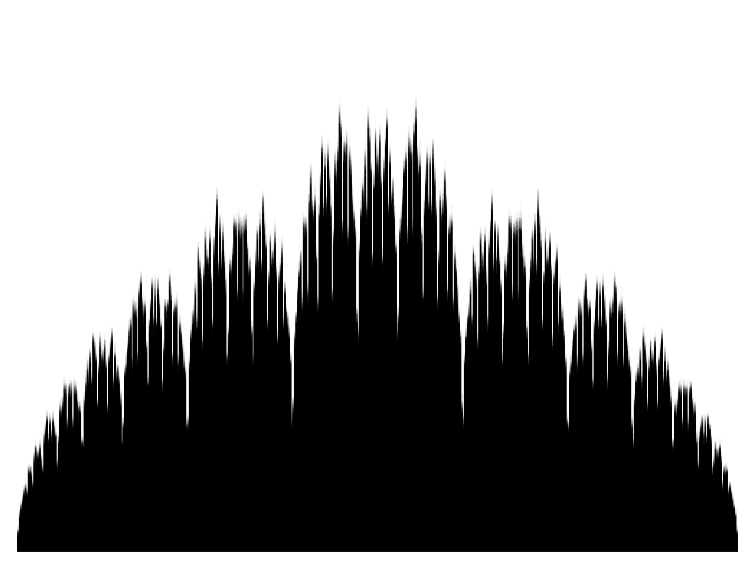
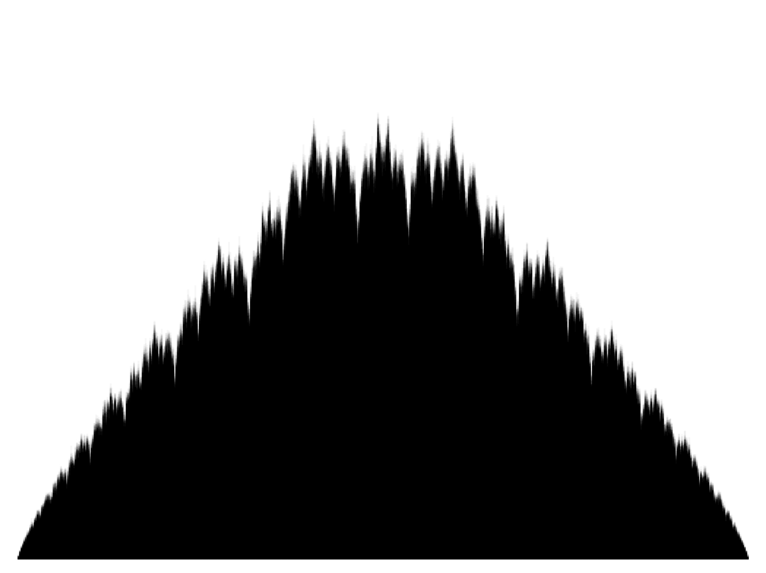
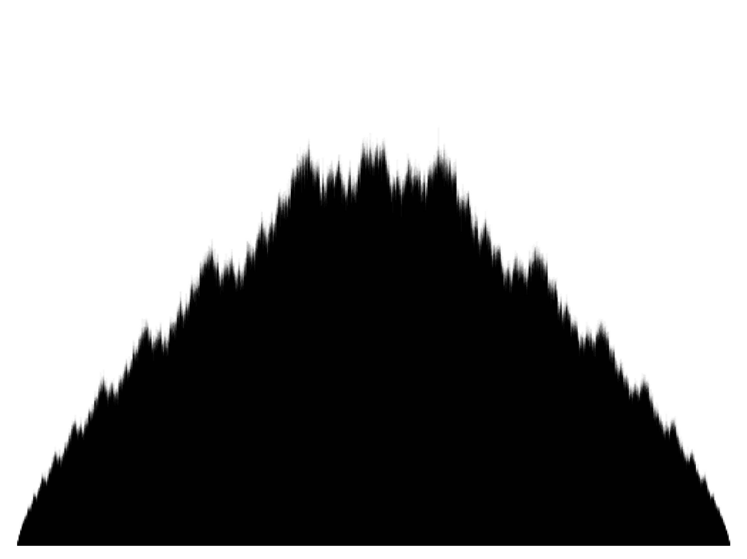
Refer to caption
(a) λ=5120.618𝜆512similar-to-or-equals0.618\lambda=\frac{\sqrt{5}-1}{2}\simeq 0.618
Refer to caption
(b) λ=e40.680𝜆𝑒4similar-to-or-equals0.680\lambda=\frac{e}{4}\simeq 0.680
Refer to caption
(c) λ=230.667𝜆23similar-to-or-equals0.667\lambda=\frac{2}{3}\simeq 0.667
Figure 1: Histogram of the empirical distribution of the Markov chain associated to (T0,T1)subscript𝑇0subscript𝑇1(T_{0},T_{1}), with X0=0subscript𝑋00X_{0}=0, binned in 500500500 subintervals (averaged image over 303030 independent runs of 106superscript10610^{6} points each). Parameter λ𝜆\lambda is the inverse of a Pisot number on the left, a very well approximable irrational at the center, rational on the right.

One can realize naturally βλsubscript𝛽𝜆\beta_{\lambda} as the stationary law of the Markov transition kernel 𝖬=(mx)x𝖬subscriptsubscript𝑚𝑥𝑥\mathsf{M}=(m_{x})_{x\in\mathbb{R}} defined by

mx=12δT0(x)+12δT1(x)subscript𝑚𝑥12subscript𝛿subscript𝑇0𝑥12subscript𝛿subscript𝑇1𝑥m_{x}=\frac{1}{2}\delta_{T_{0}(x)}+\frac{1}{2}\delta_{T_{1}(x)}

where T0(x)=λxλsubscript𝑇0𝑥𝜆𝑥𝜆T_{0}(x)=\lambda x-\lambda and T1(x)=λx+λsubscript𝑇1𝑥𝜆𝑥𝜆T_{1}(x)=\lambda x+\lambda (this is a particular case of an Iterated Function System).

In order to evaluate βλ(φ)subscript𝛽𝜆𝜑\beta_{\lambda}(\varphi) by a MCMC method, one cannot use the methods developed for ergodic Markov chains since, conditionally to X0=xsubscript𝑋0𝑥X_{0}=x, the law mxksuperscriptsubscript𝑚𝑥𝑘m_{x}^{k} of Xksubscript𝑋𝑘X_{k} is atomic and thus singular with respect to βλsubscript𝛽𝜆\beta_{\lambda}: dTV(mxk,βλ)=1subscript𝑑TVsuperscriptsubscript𝑚𝑥𝑘subscript𝛽𝜆1d_{\mathrm{TV}}(m_{x}^{k},\beta_{\lambda})=1 for all k𝑘k. The convergence only holds for observables satisfying some regularity assumption, and it is natural to ask what regularity is needed.

For a Lipschitz observable φ𝜑\varphi one only need to observe that 𝖬𝖬\mathsf{M} has positive curvature in the sense of Ollivier (this is easy using the coupling 12δ(T0(x),T0(y))+12δ(T1(x),T1(y))12subscript𝛿subscript𝑇0𝑥subscript𝑇0𝑦12subscript𝛿subscript𝑇1𝑥subscript𝑇1𝑦\frac{1}{2}\delta_{(T_{0}(x),T_{0}(y))}+\frac{1}{2}\delta_{(T_{1}(x),T_{1}(y))} of mxsubscript𝑚𝑥m_{x} and mysubscript𝑚𝑦m_{y}) and apply [JO10]. But what if φ𝜑\varphi is not Lipschitz (or has large Lipschitz constant)? We shall consider observables of bounded variation, a regularity which has the great advantage over Lipschitz to include the characteristic functions of intervals.

Definition 4.1.

Given an interval I𝐼I\subset\mathbb{R}, we consider the Banach space BV(I)BV𝐼\operatorname{BV}(I) of bounded variation functions I𝐼I\to\mathbb{R}, defined by the norm BV=+var(,I)subscriptdelimited-∥∥BVsubscriptdelimited-∥∥var𝐼\lVert\cdot\rVert_{\operatorname{BV}}=\lVert\cdot\rVert_{\infty}+\operatorname{var}(\cdot,I) where

var(f,I):=supx0<x1<<xpIj=1p|f(xj)f(xj1)|assignvar𝑓𝐼subscriptsupremumsubscript𝑥0subscript𝑥1subscript𝑥𝑝𝐼superscriptsubscript𝑗1𝑝𝑓subscript𝑥𝑗𝑓subscript𝑥𝑗1\operatorname{var}(f,I):=\sup_{x_{0}<x_{1}<\dots<x_{p}\in I}\sum_{j=1}^{p}\lvert f(x_{j})-f(x_{j-1})\rvert

(the uniform norm is usually replaced by the L1superscript𝐿1L^{1} norm, but when I𝐼I is bounded our choice is equivalent up to a constant, it does not single out the Lebesgue measure, and most importantly it ensures that BV(I)BV𝐼\operatorname{BV}(I) is a Banach algebra).

Important features of total variation are:

  • its extensiveness: var(f,I)var(f,J)+var(f,K)var𝑓𝐼var𝑓𝐽var𝑓𝐾\operatorname{var}(f,I)\geq\operatorname{var}(f,J)+\operatorname{var}(f,K) whenever J,K𝐽𝐾J,K are disjoint subintervals of I𝐼I,

  • its invariance under monotonic maps: var(fT,I)=var(f,T(I))var𝑓𝑇𝐼var𝑓𝑇𝐼\operatorname{var}(f\circ T,I)=\operatorname{var}(f,T(I)) whenever T𝑇T is monotonic.

It turns out that the averaging operator L0subscriptL0\mathrm{L}_{0} of the transition kernel 𝖬𝖬\mathsf{M} has a spectral gap for all λ𝜆\lambda, but is not a contraction when λ>1/2𝜆12\lambda>1/2 (i.e. we have an inequality L0n(f)C(1δ0)nfdelimited-∥∥superscriptsubscriptL0𝑛𝑓𝐶superscript1subscript𝛿0𝑛delimited-∥∥𝑓\lVert\mathrm{L}_{0}^{n}(f)\rVert\leq C(1-\delta_{0})^{n}\lVert f\rVert on a closed hyperplane, but with C>1𝐶1C>1). In yet other words, an iterate of L0subscriptL0\mathrm{L}_{0} is a contraction, and to apply directly Theorems A and B we need to consider an extracted Markov chain (Xk)k0subscriptsubscript𝑋𝑘𝑘0(X_{\ell k})_{k\geq 0} for some \ell.

Let Iλsubscript𝐼𝜆I_{\lambda} be the attractor of the IFS (T0,T1)subscript𝑇0subscript𝑇1(T_{0},T_{1}), i.e. the interval whose endpoints are the fixed points of T0subscript𝑇0T_{0} and T1subscript𝑇1T_{1}:

Iλ=[λ1λ,λ1λ].subscript𝐼𝜆𝜆1𝜆𝜆1𝜆I_{\lambda}=\big{[}\frac{-\lambda}{1-\lambda},\frac{\lambda}{1-\lambda}\big{]}.

Given a word ω=ω1ω2ωk𝜔subscript𝜔1subscript𝜔2subscript𝜔𝑘\omega=\omega_{1}\omega_{2}\dots\omega_{k} in the letters 00 and 111, we define

Tω=Tω1Tω2Tωk:IλIλ.:subscript𝑇𝜔subscript𝑇subscript𝜔1subscript𝑇subscript𝜔2subscript𝑇subscript𝜔𝑘subscript𝐼𝜆subscript𝐼𝜆T_{\omega}=T_{\omega_{1}}\circ T_{\omega_{2}}\circ\dots\circ T_{\omega_{k}}:I_{\lambda}\to I_{\lambda}.
Theorem 4.2.

If λ<12superscript𝜆12\lambda^{\ell}<\frac{1}{2}, then L0superscriptsubscriptL0\mathrm{L}_{0}^{\ell} has a spectral gap on BV(Iλ)BVsubscript𝐼𝜆\operatorname{BV}(I_{\lambda}) of size 1/(2+11)1superscript2111/(2^{\ell+1}-1) and constant 111.

Proof.

Let Iλ,Iλ+superscriptsubscript𝐼𝜆superscriptsubscript𝐼𝜆I_{\lambda}^{-},I_{\lambda}^{+} be the left and right halves of Iλsubscript𝐼𝜆I_{\lambda}, i.e. Iλ=[λ1λ,0)superscriptsubscript𝐼𝜆𝜆1𝜆0I_{\lambda}^{-}=\big{[}\frac{-\lambda}{1-\lambda},0\big{)} and Iλ+=(0,λ1λ]superscriptsubscript𝐼𝜆0𝜆1𝜆I_{\lambda}^{+}=\big{(}0,\frac{\lambda}{1-\lambda}\big{]}.

Let fBV(Iλ)𝑓BVsubscript𝐼𝜆f\in\operatorname{BV}(I_{\lambda}) and observe that the condition λ<12superscript𝜆12\lambda^{\ell}<\frac{1}{2} ensures that T000(Iλ)subscript𝑇000subscript𝐼𝜆T_{00\dots 0}(I_{\lambda}) and T111(Iλ)subscript𝑇111subscript𝐼𝜆T_{11\dots 1}(I_{\lambda}) are disjoint (they have length <12|Iλ|absent12subscript𝐼𝜆<\frac{1}{2}\lvert I_{\lambda}\rvert and each contains an endpoint of Iλsubscript𝐼𝜆I_{\lambda}). Then:

var(L0f,Iλ)varsuperscriptsubscriptL0𝑓subscript𝐼𝜆\displaystyle\operatorname{var}(\mathrm{L}_{0}^{\ell}f,I_{\lambda}) 12ω{0,1}var(fTω,Iλ)12ω{0,1}var(f,Tω(Iλ))absent1superscript2subscript𝜔superscript01var𝑓subscript𝑇𝜔subscript𝐼𝜆1superscript2subscript𝜔superscript01var𝑓subscript𝑇𝜔subscript𝐼𝜆\displaystyle\leq\frac{1}{2^{\ell}}\sum_{\omega\in\{0,1\}^{\ell}}\operatorname{var}(f\circ T_{\omega},I_{\lambda})\leq\frac{1}{2^{\ell}}\sum_{\omega\in\{0,1\}^{\ell}}\operatorname{var}(f,T_{\omega}(I_{\lambda}))
12(var(f,T000(Iλ))+var(f,T111(Iλ)+ω000111var(f,Iλ))\displaystyle\leq\frac{1}{2^{\ell}}\Big{(}\operatorname{var}(f,T_{00\dots 0}(I_{\lambda}))+\operatorname{var}(f,T_{11\dots 1}(I_{\lambda})+\sum_{\begin{subarray}{c}\omega\neq 00\dots 0\\ \phantom{\omega}\neq 11\dots 1\end{subarray}}\operatorname{var}(f,I_{\lambda})\Big{)}
12(var(f,Iλ)+(22)var(f,Iλ))absent1superscript2var𝑓subscript𝐼𝜆superscript22var𝑓subscript𝐼𝜆\displaystyle\leq\frac{1}{2^{\ell}}\big{(}\operatorname{var}(f,I_{\lambda})+(2^{\ell}-2)\operatorname{var}(f,I_{\lambda})\big{)}
var(L0f,Iλ)varsuperscriptsubscriptL0𝑓subscript𝐼𝜆\displaystyle\operatorname{var}(\mathrm{L}_{0}^{\ell}f,I_{\lambda}) (12)var(f,Iλ).absent1superscript2var𝑓subscript𝐼𝜆\displaystyle\leq(1-2^{-\ell})\operatorname{var}(f,I_{\lambda}).

Applying Lemma 1.1 with C=1𝐶1C=1 and θ=12𝜃1superscript2\theta=1-2^{-\ell} yields the claim. ∎

This enables us to apply our result to estimate βλ(φ)subscript𝛽𝜆𝜑\beta_{\lambda}(\varphi) for any φ𝜑\varphi of bounded variation. For example, Theorem A yields the following.

Corollary 4.3.

Let λ(12,1)𝜆121\lambda\in(\frac{1}{2},1) and let \ell be an integer such that λ<12superscript𝜆12\lambda^{\ell}<\frac{1}{2}. Consider a Markov chain (Xk)k0subscriptsubscript𝑋𝑘𝑘0(X_{k})_{k\geq 0} with transition probability 2superscript22^{-\ell} from xIλ𝑥subscript𝐼𝜆x\in I_{\lambda} to Tω(x)subscript𝑇𝜔𝑥T_{\omega}(x), for each ω{0,1}𝜔superscript01\omega\in\{0,1\}^{\ell}. For any starting distribution X0μsimilar-tosubscript𝑋0𝜇X_{0}\sim\mu, any φBV(Iλ)𝜑BVsubscript𝐼𝜆\varphi\in\operatorname{BV}(I_{\lambda}), any positive a<φBV/3(2+11)𝑎subscriptdelimited-∥∥𝜑BV3superscript211a<\lVert\varphi\rVert_{\operatorname{BV}}/3(2^{\ell+1}-1) and any n1202𝑛120superscript2n\geq 120\cdot 2^{\ell} we have

μ[|μ^n(φ)μ0(φ)|a]2.488exp(na2φBV2(16.652+5.12)).subscript𝜇subscript^𝜇𝑛𝜑subscript𝜇0𝜑𝑎2.488𝑛superscript𝑎2superscriptsubscriptdelimited-∥∥𝜑BV216.65superscript25.12\operatorname{\mathbb{P}}_{\mu}\Big{[}\lvert\hat{\mu}_{n}(\varphi)-\mu_{0}(\varphi)\rvert\geq a\Big{]}\leq 2.488\exp\Big{(}-\frac{na^{2}}{\lVert\varphi\rVert_{\operatorname{BV}}^{2}(16.65\cdot 2^{\ell}+5.12)}\Big{)}.

To the best of our knowledge, this example could not be handled effectively by previously known results. For example [GD12] needs the observable to be at least C2superscript𝐶2C^{2} to have explicit estimates, and they do not give a concentration inequality.

References

  • [GD12] David M Gómez and Pablo Dartnell, Simple monte carlo integration with respect to Bernoulli convolutions, Applications of Mathematics 57 (2012), no. 6, 617–626.
  • [GO02] Peter W Glynn and Dirk Ormoneit, Hoeffding’s inequality for uniformly ergodic Markov chains, Statistics & probability letters 56 (2002), no. 2, 143–146.
  • [JO10] Aldéric Joulin and Yann Ollivier, Curvature, concentration and error estimates for Markov chain Monte Carlo, Ann. Probab. 38 (2010), no. 6, 2418–2442. MR 2683634
  • [KLMM05] Ioannis Kontoyiannis, Luis A Lastras-Montano, and Sean P Meyn, Relative entropy and exponential deviation bounds for general Markov chains, International Symposium on Information Theory, 2005, IEEE, 2005, pp. 1563–1567.
  • [Klo17] Benoît R. Kloeckner, Effective limit theorems for Markov chains with a spectral gap, arXiv:1703.09623, 2017.
  • [Oll09] Yann Ollivier, Ricci curvature of Markov chains on metric spaces, J. Funct. Anal. 256 (2009), no. 3, 810–864. MR 2484937
  • [Pau15] Daniel Paulin, Concentration inequalities for Markov chains by Marton couplings and spectral methods, Electronic Journal of Probability 20 (2015).
  • [Pet17] Fedor Petrov, Answer to “diameter of a weighted Hamming cube”, MathOverflow, 2017, https://mathoverflow.net/a/286346/4961.
  • [PSS00] Yuval Peres, Wilhelm Schlag, and Boris Solomyak, Sixty years of Bernoulli convolutions, Progress in probability (2000), 39–68.