Facing to Latency of Hyperledger Fabric for
Blockchain-enabled IoT: Modeling and Analysis

Abstract

Hyperledger Fabric (HLF), one of the most popular private blockchains, has recently received attention for blockchain-enabled Internet of Things (IoT). However, for IoT applications to handle time-sensitive data, the processing latency in HLF has emerged as a new challenge. In this article, therefore, we establish a practical HLF latency model for HLF-enabled IoT. We first discuss the structure and transaction flow of HLF-enabled IoT. After implementing real HLF, we capture the latencies that each transaction experiences and show that the total latency of HLF can be modeled as a Gamma distribution, which is validated by conducting a goodness-of-fit test (i.e., the Kolmogorov-Smirnov (KS) test). We also provide the parameter values of the modeled latency distribution for various HLF environments. Furthermore, we explore the impacts of three important HLF parameters including transaction generation rate, block size, and block-generation timeout on the HLF latency. As a result, this article provides design insights on minimizing the latency for HLF-enabled IoT.

I Introduction

Since blockchain technology was developed as a novel solution to ensure data integrity in distributed systems, various blockchain-enabled Internet of Things (IoT) applications have recently emerged. In the blockchain-enabled IoT applications, delivered IoT data is appended to the assigned remote blockchain storage. Blockchains can be classified into two types: public blockchain and private blockchain. The private blockchain has recently received much attention in terms of fast transaction processing and privacy preservation [1]. Particularly, Hyperledger Fabric (HLF), which is hosted by Linux Foundation and contributed by IBM since 2015, is gaining popularity [2] as one of the promising private blockchains. As discovered in literature [3, 4, 5], HLF-enabled IoT applications include industrial IoT (IIoT), healthcare, wireless monitoring, and unmanned aerial vehicles. For example, decentralized IoT data marketplace is proposed using HLF in [3]. For smart healthcare, HLF is exploited for IoT to share monitored patient vital signs [4] and to ensure security and privacy for medical data in the Healthcare 4.0 industry using UAVs [5]. Thus, it is expected that HLF will be more widely used to securely manage a high volume of IoT data.

However, in blockchain platforms including HLF, high latency is still recognized as a major issue [2]. Specifically, certain IoT applications, which are handling time-critical data, may have strict latency requirements for making correct and useful decision [6], and require fast transaction commitment. For example, vital signs of patients need to be promptly processed and transferred to smart hospital blockchain networks for effective medical care [4]. Therefore, for those applications, it is important to predict and understand the HLF latency, prior to their practical implementations. Nonetheless, in most works on HLF-enabled applications, the HLF latency is generally not considered or simply ignored, and the latency characteristics including its distribution have not been fully explored.

Recently, there have been some works that analyze the HLF latency such as the ones for HLF v0.6 [7] and the ones for HLF v1.0 or higher [8, 9, 10, 11]. Specifically, a stochastic reward net (SRN) model is used to define the latency of HLF v0.6 in [7]. For HLF v1.0 or higher, by considering Kafka/ZooKeeper, which is a new consensus algorithm released in HLF v1.0, the latency is defined and measured based on several theoretical models including SRN [8], generalized stochastic petri nets [9], a hierarchical model based on transaction execution and validation [10], and a queueing-based model [11].

However, in all above HLF latency studies, only the mean latency is presented without showing the latency distribution, and in most works, the theoretical models are not verified in real HLF. When the latency is measured from real implementation of HLF, it is quite random, so the distribution of the latency is importantly required for the design of reliable HLF-enabled IoT. Furthermore, HLF has a sophisticated structure, where many network parameters affect the latency simultaneously, so their impacts on the latency should be carefully investigated to lower the HLF latency.

In this article, therefore, we establish a latency model of HLF especially for HLF-enabled IoT, where time-sensitive data is generally managed. After characterizing the latency distribution, we also analyze the impacts of three important HLF parameters (i.e., block size, block-generation timeout, and transaction generation rate) on the HLF latency. We then discuss how the HLF latency can be reduced by setting those parameters properly. The contributions of this article can be summarized as follows:

• We newly provide the probability distribution of the HLF latency by performing the probability distribution fitting on transaction latency samples, which are captured in real HLF. We also provide the parameter values of corresponding probability distributions for various HLF parameter setups. To the best of our knowledge, this is the first work that provides the distribution of the HLF latency.

• We develop the latency model of HLF with a new structure, which is adopted in the latest HLF releases. Hence, our work is more compatible with current HLF-enabled IoT, compared to the previous HLF latency model for HLF v0.6 [7].

• We explore the impacts of three main HLF parameters (i.e., block size, block-generation timeout, and transaction generation rate) on the HLF latency. Especially, we figure out the existence of the best values of those HLF parameters that minimize the HLF latency. This provides some design insights on HLF parameters to lower the HLF latency for more reliable HLF-enabled IoT.

II HLF-enabled IoT

HLF is a private blockchain platform for a modular architecture, which is one of the sub-projects in the Hyperledger Project. In the other blockchain platforms, a deterministic programming language is compulsory to prohibit their ledgers from diverging, such as Solidity in Ethereum. In contrast, the novel structure of HLF v1.0 or higher not only enables general-purpose programming languages, but also prevents ledger bifurcation at the same time. In this section, we first describe a basic structure of HLF-enabled IoT. We then demonstrate the transaction flow consisting of three phases, and provide the definitions of some important parameters in HLF. Note that more detailed explanations of HLF are provided in [12].

II-A HLF-enabled IoT Structure

Figure 1 shows the basic structure of HLF-enabled IoT, where the data, delivered from IoT devices, are stored and managed by HLF. Note that HLF can support multiple IoT applications, but it can provide an independent ledger for each application for data confidentiality. Thus, each IoT application can maintain its ledger without unauthorized access. As shown in Fig. 1, the data from an IoT device is transmitted through a base station (BS) or an access point (AP). The data is then appended to the ledger in HLF by following the transaction flow, which will be described in Section II-B.

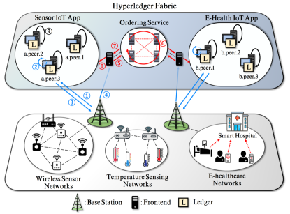
Figure 1: Structure of HLF-enabled IoT.

II-B Transaction Flow

Transactions in HLF are appended to the ledger through three phases: endorsing phase, ordering phase, and validation phase. The processing phases enable HLF networks not only to support general-purpose programming languages, but also to remain tamper-proof. In this subsection, we describe the transaction flow in HLF for data updates.

II-B1 Endorsing Phase

The endorsing phase is to ensure that endorsing peers have the same transaction execution results obtained from each of their copied ledgers. This phase is necessary to prevent blockchain forks. If they are identical, the transaction is delivered to the ordering service. In contrast, the transaction is discarded if they are different.

II-B2 Ordering Phase

The ordering phase is to order all transactions chronologically and generate new blocks in the ordering service. Note that the ordering service is a node cluster, where a pre-defined consensus protocol is conducted. A newly generated block is transmitted to peers for the validation phase through the gossip protocol. Note that we focus on the Kafka/ZooKeeper-based ordering service, which is currently the most widely used [13].

II-B3 Validation Phase

The validation phase is the last phase in which the new block is validated by each peer individually. In this phase, a receiving peer mainly conducts sequential verification processes on each transaction in the block, in the order described in [12]. If any of the verification processes is violated at a transaction, it is marked as invalid and prohibited from updating the ledger.

II-C Important HLF Parameters

In this subsection, we define three important HLF parameters, which mainly affect the HLF latency.

II-C1 Block Size

The block size $S_{\text{b}}$ is one of the configurable parameters of the ordering service. This parameter defines the maximum number of transactions in one block. In other words, the block size determines how many transactions the ordering service can collect the most in one block. The transactions are promptly exported from the ordering service as a new block, when the number of transactions in the waiting queue reaches a pre-defined block size value.

II-C2 Block-generation Timeout

The block-generation timeout $T_{\text{b}}$ is another configurable parameter of the ordering service. This parameter defines the maximum time to wait for other transactions to be exported as a new block since the first transaction arrived at the waiting queue. Once the timer expires, the waiting transactions are included into a new block, regardless of their number in the waiting queue.

II-C3 Transaction Generation Rate

The transaction generation rate $\lambda_{\text{t}}$ refers to the number of transactions arrived in HLF per second. Being different from the two configurable parameters above, this parameter can be determined by many factors. For example, when an IoT device conveys data to HLF as transactions, the communication channel and data generation frequency of the device can affect this parameter.

\psfrag{XXX}[Bc][bc][0.8]{$t$ [sec]}\psfrag{YYY}[Bc][bc][0.8]{Probability/$\Delta_{t}$}\includegraphics[width=433.62pt]{figures/el_t1b10r10.eps}

(a) Endorsing latency:
Exponential dist. PDF
$[\lambda=94.5]$

\psfrag{XXX}[Bc][bc][0.8]{$t$ [sec]}\psfrag{YYY}[Bc][bc][0.8]{Probability/$\Delta_{t}$}\includegraphics[width=433.62pt]{figures/ol_t1b10r10.eps}

(b) Ordering latency:
Gamma dist. PDF
$[\alpha_{\text{o}}=2.652,\beta_{\text{o}}=3.458]$

\psfrag{XXX}[Bc][bc][0.8]{$t$ [sec]}\psfrag{YYY}[Bc][bc][0.8]{Probability/$\Delta_{t}$}\psfrag{Hist}[Bl][Bl][0.7]{Validation latency histogram}\includegraphics[width=433.62pt]{figures/vl_t1b10r10.eps}

(c) Validation latency:
Fréchet dist. PDF
$[\alpha=0.21,s=0.479,m=0.144]$

\psfrag{XXX}[Bc][bc][0.8]{$t$ [sec]}\psfrag{YYY}[Bc][bc][0.8]{Probability/$\Delta_{t}$}\includegraphics[width=433.62pt]{figures/lc_t1b10r10.eps}

(d) Total latency:
Gamma dist. PDF
$[\alpha_{\text{t}}=7.362,\beta_{\text{t}}=5.445]$

Figure 2: Histograms (blue bars) and their best-fit distributions (red lines) of the endorsing latency, ordering latency, validation latency, and ledger-commitment latency, where $S_{\text{b}}=10$, $T_{\text{b}}=1$ [sec], and $\lambda_{\text{t}}=10$ transactions/second.

III HLF Latency Modeling

In this section, we conduct HLF latency modeling based on the probability distribution fitting method. We first define latency types in HLF, and provide the experimental setup of our HLF networks. For the probability distribution fitting method, we first capture transaction latency samples from the HLF networks. We then the best fit distribution for each latency type, and finally provide our HLF latency model. For evaluating goodness-of-fit of our modeling, we also conduct the Kolmogorov-Smirnov (KS) test. The feasibility conditions for our latency modeling are discussed with providing the cases, for which the probability distribution fitting method does not work well.

III-A Latency Types in HLF

Before modeling the HLF latency, we first divide the total elapsed time of the data in the HLF network according to the transaction-processing stages, described in Section II-B, such as the endorsing latency, the ordering latency, the validation latency, and the ledger-commitment latency (i.e., the total latency). Note that we exclude the communication latency spent from an IoT device to reach the HLF network, as it is more depending on the communication standard that IoT devices use, and it has already been explored in many literature.

III-A1 Endorsing Latency

The endorsing latency refers to the time taken to request endorsing peers to endorse a transaction, and to receive their responses. To be specific, it is defined as the sum of the latencies for step 1, 2, 3, and 4 in Fig. 1.

III-A2 Ordering Latency

The ordering latency refers to the time taken to await until the transaction is exported as a new block from the ordering service. It is defined as the sum of the latencies for step 5, 6, 7, and 8 in Fig. 1. Note that the latency for step 6 consists of the consensus time and the waiting time for other transactions to be released as part of a new block. In contrast, the latency for step 8 is the sum of transmission time and the waiting time of the released block for the validation phase. Thus, it may be considered as part of the validation latency. In this article, however, we include this latency into the ordering latency, when we depict the histograms in Figs. 2 and 4. Note that the latency for step 8 may be highly likely to work as a bottleneck if the previous block requires long time to be validated.

III-A3 Validation Latency

The validation latency refers to the time taken to validate and commit the block with ledger update. This latency is defined as the latency for step 9 in Fig. 1. All transactions in the same block are sequentially validated, but committed to the ledger all together as a batch. Therefore, they have the identical validation latency from each other. Note that the validation latency may vary according to peer’s type. In this article, this latency is measured at the endorsing peer.

III-A4 Ledger-commitment Latency (Total Latency)

The ledger-commitment latency refers to the time taken to completely process a transaction from the beginning. Thus, it is the sum of the endorsing, ordering, and validation latencies.

III-B Experiment Setup

For the implementation of our HLF network, we exploit the HLF v1.3 sample network on one physical machine. The machine running the HLF network is with Intel® Xeon W-2155 @ 3.30 GHz processor and 16 GB RAM. In addition, we newly bring up a Kafka/ZooKeeper-based ordering service consisting of four Kafka nodes, three ZooKeeper nodes, and three frontend nodes that are connected to the Kafka node cluster in the network (i.e., the minimum number of required Kafka and ZooKeeper nodes for crash fault tolerance). Note that the frontend node is not only to inject transactions from clients into the Kafka node cluster, but also to receive new blocks, which will be disseminated to peers. The HLF network has one endorsing peer and two committing peers. Note that the number of committing peers may not affect the ledger-commitment latency because they only validate newly delivered blocks and hold copied ledgers.

We perform 10 test runs for one experiment setup, and each test run includes 1,000 transaction proposals transmitted. All proposals attempt to update a key-value set, using appropriate parameters for the changeCarOwner function defined in the Fabcar chaincode. Each of the equipped frontend nodes has an equal probability of being selected to relay a transaction from our client to the Kafka node cluster, and to make a new block propagated. Note that the generated proposals in one test run do not access the same key-value set. Hence, we do not consider the multi-version concurrency control (MVCC) violation during the validation phase in this article.

New transactions are generated at the rate of $\lambda_{\text{t}}$ transactions/second, and their inter-generation times follow an exponential distribution. At each iteration of test runs, we not only vary the transaction generation rate $\lambda_{\text{t}}$, but also measure the endorsing, ordering, validation, and ledger-commitment latency in order to analyze the impact of increasing $\lambda_{\text{t}}$. Note that $S_{\text{b}}$ and $T_{\text{b}}$ refer to the block size and block-generation timeout, respectively.

III-C Latency Modeling

For the latency modeling, we first obtain the histogram for each latency type defined in Section III-A, and then figure out its best-fit probability distribution. The discovered best-fit distributions are as follows.

III-C1 Endorsing Latency

The best-fit distribution of the endorsing latency is the exponential distribution $T_{\text{e}}\sim\text{Exp$(\lambda)$}$, whose probability density function (PDF) is defined as

$$f_{T_{\text{e}}}(t)={\lambda}e^{-\lambda t},$$ (1)

where $\lambda=\frac{1}{\mathbb{E}[T_{\text{e}}]}$ is the rate parameter for $\lambda>0$. Note that the cumulative distribution function (CDF) of the endorsing latency is $F_{T_{\text{e}}}(t)=1-e^{-\lambda t}$.

III-C2 Ordering and Ledger-commitment Latencies

The best-fit distributions of the ordering latency and ledger-commitment latency are the Gamma distribution, $T_{\text{o}}\sim\text{Gamma$(\alpha_{\text{o}},\beta_{\text{o}})$}$ and $T_{\text{t}}\sim\text{Gamma$(\alpha_{\text{t}},\beta_{\text{t}})$}$ respectively, whose PDF is defined as

$$f_{T_{i}}(t)=\frac{{\beta_{i}}^{\alpha_{i}}}{\Gamma(\alpha_{i})}t^{{\alpha_{i}}-1}e^{-{\beta_{i}}t},$$ (2)

where $i$ is an indicator for the ordering latency $(i=\text{o})$ and for the ledger-commitment latency $(i=\text{t})$, $\Gamma(\alpha_{i})=\int_{0}^{\infty}x^{\alpha_{i}-1}\,e^{-x}\,\text{d}x$ is the gamma function, and $\gamma(\alpha_{i},\beta_{i}t)=\int_{0}^{\beta_{i}t}x^{\alpha_{i}-1}\,e^{-x}\,\text{d}x$ is the lower incomplete gamma function for $t\geq 0$. Note that $\alpha_{\text{o}}=\beta_{\text{o}}\mathbb{E}[T_{\text{o}}]$ and $\alpha_{\text{t}}=\beta_{\text{t}}\mathbb{E}[T_{\text{t}}]$, where $\alpha_{\text{o}}$ and $\alpha_{\text{t}}$ are the shape parameters and $\beta_{\text{o}}$ and $\beta_{\text{t}}$ are the inverse scale parameters (i.e., the rate parameters). The CDFs of the ordering and ledger-commitment latencies are $F_{T_{i}}(t)=\frac{1}{\Gamma(\alpha_{i})}{\gamma({\alpha_{i}},{\beta_{i}}t)}$.

TABLE I: Estimated Gamma distribution parameters ($\alpha_{\text{t}},\beta_{\text{t}}$), the KS test results, the average latency of empirical results $\overline{T}_{\text{ep}}$, and the average latency of the best-fit distribution $\overline{T}_{\text{bf}}$ for the ledger-commitment latency.

$S_{\text{b}}$	$T_{\text{b}}$	$\lambda_{\text{t}}$	Estimated $(\alpha_{\text{t}},\beta_{\text{t}})$	KS Statistics	Empirical Avg. $\overline{T}_{\text{ep}}$	Best-fit Avg. $\overline{T}_{\text{bf}}$
20	1	10	(8.9573, 5.5858)	0.0457	1.6066	1.6035
		11	(9.5112, 6.0407)	0.0466	1.5767	1.5745
		12	(9.3159, 6.2078)	0.0503	1.4969	1.5006
		13	(10.0333, 6.2937)	0.049	1.5891	1.5941
25	1	17	(9.7902, 6.0267)	0.0504	1.6141	1.6244
		18	(9.1368, 6.131)	0.0595	1.4908	1.4902
		19	(9.005, 5.9462)	0.0564	1.5098	1.5144
		20	(8.2069, 5.395)	0.051	1.5232	1.5212
10	2	8	(7.181, 4.0151)	0.0388	1.8289	1.7884
		9	(6.8603, 4.6625)	0.0437	1.4658	1.4713
		10	(5.6829, 4.355)	0.0457	1.3517	1.3049
		11	(7.1636, 4.1801)	0.0444	1.7513	1.7137
20	2	15	(7.6898, 4.6474)	0.0358	1.6587	1.6566
		16	(8.4486, 5.1794)	0.0474	1.6406	1.6311
		17	(8.0874, 5.2866)	0.0419	1.5323	1.5297
		18	(8.3269, 4.8638)	0.0404	1.7437	1.712
20	3	15	(7.9739, 4.9723)	0.0382	1.616	1.6036
		16	(7.608, 4.9499)	0.0394	1.5351	1.537
		17	(7.0015, 4.9697)	0.0403	1.3992	1.4088
		18	(5.7078, 4.1482)	0.0513	1.3902	1.3759
30	3	23	(8.0788, 4.6915)	0.0369	1.727	1.722
		24	(7.0546, 4.527)	0.0395	1.5652	1.5583
		25	(6.3698, 4.4257)	0.0468	1.4345	1.4392
		26	(7.3836, 4.8698)	0.0435	1.5125	1.5162
9	2	10	(8.9573, 5.5858)	0.0457	1.6066	1.6035
10			(9.5112, 6.0407)	0.0466	1.5767	1.5745
12			(9.3159, 6.2078)	0.0503	1.4969	1.5006
15			(10.0333, 6.2937)	0.049	1.5891	1.5941
10	1.75	10	(9.7902, 6.0267)	0.0504	1.6141	1.6244
	2.00		(9.1368, 6.131)	0.0595	1.4908	1.4902
	2.25		(9.005, 5.9462)	0.0564	1.5098	1.5144
	2.50		(8.2069, 5.395)	0.051	1.5232	1.5212

III-C3 Validation Latency

The best-fit distribution of the validation latency is the three-parameter Fréchet distribution $T_{\text{v}}\sim\text{Frechet$(\alpha,s,m)$}$, whose PDF is defined as [14]

$$f_{T_{\text{v}}}(t)=\frac{\alpha}{s}\left(\frac{t-m}{s}\right)^{-1-\alpha}e^{-\left(\frac{t-m}{s}\right)^{-\alpha}},$$ (3)

where $\alpha$, $s$, and $m$ are the shape, scale, and location parameters, respectively, for $0<\alpha<\infty$, $0<s<\infty$, and $-\infty<m<\infty$. Note that the CDF of the validation latency is $F_{T_{\text{v}}}(t)=e^{-\left(\frac{t-m}{s}\right)^{-\alpha}}$.

\psfrag{XXX}[Bc][bc][0.8]{$t$ [sec]}\psfrag{YYY}[Bc][bc][0.8]{Cumulative distribution function $F_{T_{\text{t}}}(t)$}\psfrag{DDDDDDDDDDDDDDDDDDDl}[Bl][Bl][0.7]{Empirical results, $\lambda_{\text{t}}=8$}\psfrag{data2}[Bl][Bl][0.7]{Best-fit distribution, $\lambda_{\text{t}}=8$}\psfrag{data3}[Bl][Bl][0.7]{Empirical results, $\lambda_{\text{t}}=9$}\psfrag{data4}[Bl][Bl][0.7]{Best-fit distribution, $\lambda_{\text{t}}=9$}\psfrag{data5}[Bl][Bl][0.7]{Empirical results, $\lambda_{\text{t}}=10$}\psfrag{data6}[Bl][Bl][0.7]{Best-fit distribution, $\lambda_{\text{t}}=10$}\psfrag{data7}[Bl][Bl][0.7]{Empirical results, $\lambda_{\text{t}}=11$}\psfrag{data8}[Bl][Bl][0.7]{Best-fit distribution, $\lambda_{\text{t}}=11$}\includegraphics[width=216.81pt]{figures/t2b10cdf.eps}

Figure 3: Empirical CDFs and the best-fit Gamma distribution CDFs of the ledger-commitment latency $T_{\text{t}}$ for different values of the transaction generation rates $\lambda_{\text{t}}$, where $S_{\text{b}}=10$ and $T_{\text{b}}=2$ [sec].

Once the best-fit distributions are determined, we estimate the distribution parameters, such as $\lambda$ for the endorsing, $(\alpha,s,m)$ for the validation, and $(\alpha_{\text{o}},\beta_{\text{o}})$ and $(\alpha_{\text{t}},\beta_{\text{t}})$ for the ordering and ledger-commitment latencies, using the curve fitting tool such as the nonlinear regression method in Matlab. The histogram and discovered best-fit distribution with estimated parameter for each latency type are provided in Fig. 2. Note that $\Delta_{t}$ is the width of a bin. From Fig. 2, we can see that the discovered best-fit distributions match well with the histograms, especially with that of the ledger-commitment latency.

For the ledge-commitment latency $T_{\text{t}}$, the estimated Gamma distribution parameter pairs of the ledger-commitment latency for various HLF environments are also provided in Table I. The CDFs of some empirically measured values and their best-fit Gamma distributions are then demonstrated in Fig. 3. Note that the value of $\Delta_{t}$ does not change the shapes of histograms, so we can still use the estimated Gamma distribution parameters in Table I, even for different values of $\Delta_{t}$. In Table I, $\overline{T}_{\text{t}}$ refers to the average ledger-commitment latency for a given HLF environment. The one, obtained empirically, is denoted as $\overline{T}_{\text{ep}}$, and the one from the best-fit distribution is denoted as $\overline{T}_{\text{bf}}$.

From Fig. 3, we can see that the CDFs of the best-fit Gamma distribution matches well with the empirically obtained ones. From Table I, we can see that $\overline{T}_{\text{t}}$ decreases as $\lambda_{\text{t}}$ increases since it makes new blocks generated faster in the ordering service. However, $\overline{T}_{\text{t}}$ increases when $\lambda_{\text{t}}$ becomes higher. This is because there is a large load at the validation phase as the block-generation rate becomes higher. Hence, some blocks start to wait for the validation process, which increases $\overline{T}_{\text{t}}$.

III-D Latency Modeling Validation

In order to validate and improve the reliability of our latency model, we include KS test results in Table I. The KS test is a statistical test to evaluate goodness-of-fit based on the maximum difference between the empirical CDF of the data set and the hypothetical CDF (i.e., the CDF of the given distribution) [15].

The estimated parameters and KS statistics are averaged over ten test runs at 0.01 significance level. The critical value is computed as 0.0513. In other words, the latency model can be considered as reliable if the KS statistics value of a data set is less than 0.0513. As an example, Fig. 3 show the ledger-commitment latency, when $S_{\text{b}}=10$ and $T_{\text{b}}=2$ [sec] for $\lambda_{\text{t}}=8,9,10$ and $11$. In Table I, all cases in those figures have smaller KS statistics values (i.e., 0.0388, 0.0437, 0.0457, and 0.0444, respectively) than the critical value. Thus, the test is passed for all cases. However, in Table I, when $S_{\text{b}}=25$ and $T_{\text{b}}=1$ for $\lambda_{\text{t}}=18$ and $19$, their KS statistics values are slightly larger than the critical value, but even in those cases, we can see that they still have the similar mean latency $\overline{T}_{\text{bf}}$ to each of their $\overline{T}_{\text{ep}}$.

III-E Feasibility Conditions for Latency Modeling

During the modeling process, it is found that there exist some cases in which histograms of $\overline{T}_{\text{t}}$ do not fit well into a known probability distribution. In other words, the probability distribution fitting method is not always applicable. We have discovered two environments that make the probability distribution fitting method infeasible as follows.

III-E1 Timeout-dominant Block Generation Environment

When the transaction generation rate $\lambda_{\text{t}}$ is small, while the block-generation timeout value $T_{\text{b}}$ is relatively large, few of transactions (or even one transaction) may stay in the waiting room for the ordering service in the ordering phase most of their time, and become a block once the timeout expires. In this case, a large portion of transactions can have the ordering latency equal to $T_{\text{b}}$. As an example of such case, the histograms of the ordering latency and the ledger-commitment latency are shown in Figs. 4(a) and 4(b), respectively, where $S_{\text{b}}=10$, $T_{\text{b}}=1$ [sec], and $\lambda_{\text{t}}=3$. As shown in Fig. 4(a), there is a peak when the ordering latency is 1.2 seconds, and in this case, the percentage of blocks, which are exported from the ordering service by the block-generation timeout expiration, is 99.8%. Due to this, as shown in Fig. 4(b), the ledger-commitment latency has the distribution, which is difficult to fit using any known probability distributions.

III-E2 Block Size-dominant Block Generation Environment

When the block size $S_{\text{b}}$ is small, while the transaction generation rate $\lambda_{\text{t}}$ is large, most blocks are filled with transactions up to $S_{\text{b}}$ quickly, so blocks are generated fast with the full size from the ordering service. In this case, even though the ordering latency is small, there can be a large load at the validation phase due to the fast block generation, which makes blocks wait for validation. Hence, there can be many transactions with long waiting time to enter the validation phase. As an example of such case, the histogram of the ledger-commitment latency is provided in Fig. 4(c), where $S_{\text{b}}=15$, $T_{\text{b}}=0.75$ [sec], and $\lambda_{\text{t}}=10$. As shown in this figure, there are long-tail outliers more frequently in the distribution (e.g., the cases with the ledger-commitment latency longer than 4 seconds), which makes it difficult to fit to a known probability distribution.

Note that the two environments, discussed above, are the cases where $S_{\text{b}}$ or $T_{\text{b}}$ is too small or large, so a large portion of transactions experience long latency in the ordering or validation phase. For delay-sensitive HLF-enabled IoT, such HLF parameter setups will be generally avoided.

\psfrag{XXX}[Bc][bc][0.8]{$t$ [sec]}\psfrag{YYY}[Bc][bc][0.8]{Probability/$\Delta_{t}$}\includegraphics[width=433.62pt]{figures/ol_t1b10r3.eps}

(a) Ordering latency

\psfrag{XXX}[Bc][bc][0.8]{$t$ [sec]}\psfrag{YYY}[Bc][bc][0.8]{Probability/$\Delta_{t}$}\includegraphics[width=433.62pt]{figures/lc_t1b10r3.eps}

(b) Ledger-commitment latency

\psfrag{XXX}[Bc][bc][0.8]{$t$ [sec]}\psfrag{YYY}[Bc][bc][0.8]{Probability/$\Delta_{t}$}\includegraphics[width=433.62pt]{figures/lc_t075b15r10.eps}

(c) Ledger-commitment latency

Figure 4: Histograms of the ordering latency and the ledger-commitment latency $T_{\text{t}}$ for infeasible latency modeling cases.

IV Facing to Blockchain Latency: Influential Parameter Analysis on Latency

For HLF-enabled IoT handling time-sensitive jobs and requiring faster transaction commitment, it is important to design HLF in the way to minimize the ledger-commitment latency. We can see in Table I, $S_{\text{b}}$, $T_{\text{b}}$, and $\lambda_{\text{t}}$ affect the ledger-commitment latency. In this section, therefore, we explore their impacts on the ledger-commitment latency. Moreover, we discuss how to optimally determine the three parameters to minimize the ledger-commitment latency.

IV-A Transaction Generation Rate Control

Table I demonstrates the impact of the transaction generation rate $\lambda_{\text{t}}$ for different $S_{\text{b}}$ and $T_{\text{b}}$ on the average ledger-commitment latency $\overline{T}_{\text{t}}$ for both empirical and best-fit distribution results. From Table I, we can observe two conflicting effects of the transaction generation rate on the ledger-commitment latency. Higher $\lambda_{\text{t}}$ makes transactions exported from the ordering service faster, leading to an increase in the block-generation rate at the ordering service. Due to this, the lowest $\overline{T}_{\text{t}}$ can be achieved by increasing $\lambda_{\text{t}}$. For instance, when $S_{\text{b}}$ is $20$ and $T_{\text{b}}$ is $1$ [sec] in Table I, $\overline{T}_{\text{ep}}$ decreases from 1.6066 to 1.4969 as $\lambda_{\text{t}}$ increases from 10 to 12 transactions/second.

However, $\overline{T}_{\text{t}}$ does not continuously decrease, and starts to increase after some point of $\lambda_{\text{t}}$. As seen in Table I, when $S_{\text{b}}$ is $20$ and $T_{\text{b}}$ is $1$ [sec], $\overline{T}_{\text{ep}}$ increases from 1.4969 to 1.5891 as $\lambda_{\text{t}}$ increases from $12$ to $13$ transactions/second. This is because the block validation rate does not increase despite faster block-generation. New blocks need to wait for the validation. From these observations, we can see that the optimal $\lambda_{\text{t}}$, which minimizes $\overline{T}_{\text{t}}$, exists for a given HLF setup.

IV-B Block Size Optimization

Figure 5 illustrates the impact of the block size $S_{\text{b}}$ on $\overline{T}_{\text{t}}$ for empirical results and the best-fit distributions (red lines). Note that the probability distribution fitting results with KS statistics values are provided in Table I (see the values for $S_{\text{b}}=9,10,12,$ and $15$ and $T_{\text{b}}=2$ [sec]). From Fig. 5, we can see that the average ledger-commitment latency of the best-fit distributions are well-matched with those of the empirical results.

From Fig. 5, we can also see that when the block size $S_{\text{b}}$ is small (e.g., $S_{\text{b}}<8$), the average ledger-commitment latency $\overline{T}_{\text{t}}$ is extremely high. This is because the peers receiving blocks cannot promptly start to validate them since blocks are generated too fast due to the small block size. Therefore, new blocks gradually stack up in each peer’s queue for the validation, which leads to long validation delay. As $S_{\text{b}}$ increases, $\overline{T}_{\text{t}}$ decreases because the block-generation rate decreases and the waiting time at the validation phase becomes lower as well. However, when $S_{\text{b}}$ increases beyond certain values (e.g., $S_{\text{b}}>10$), $\overline{T}_{\text{t}}$ increases again. In this case, the validation latency is no longer long, but transactions need to wait longer for others to be included into a block in the ordering phase due to the large size of $S_{\text{b}}$. As $S_{\text{b}}$ keeps increasing, $\overline{T}_{\text{t}}$ could eventually saturate as most of the new blocks are generated by the timeout expiration before they are generated by fully collected $S_{\text{b}}$ transactions.

IV-C Block-generation Timeout Optimization

Figure 5 demonstrates the impact of the block-generation timeout $T_{\text{b}}$ on $\overline{T}_{\text{t}}$ for empirical results and the best-fit distributions (blue lines). Note that the probability distribution fitting results with KS statistics values are provided in Table I (see the values for $S_{\text{b}}=10$ and $T_{\text{b}}=1.75,2.00,2.25,$ and $2.50$ [sec]). From Fig 5, we can see that the average ledger-commitment latency of the best-fit distributions are well-matched with those of the empirical results.

From Fig. 5, we can also see that when the block-generation timeout $T_{\text{b}}$ is short (e.g., $T_{\text{b}}<1.5$ [sec]), the average ledger-commitment latency $\overline{T}_{\text{t}}$ is extremely high for the same reason as explained in Section IV-B due to the short block-generation timeout. As $T_{\text{b}}$ increases, $\overline{T}_{\text{t}}$ decreases and the waiting time at the validation phase also becomes lower. However, when $T_{\text{b}}$ increases beyond certain values (e.g., $T_{\text{b}}<2$ [sec]), $\overline{T}_{\text{t}}$ increases again. In this case, the validation latency is no longer long, but transactions need to wait longer for others to be included into a block in the ordering phase due to the long $T_{\text{b}}$. As $T_{\text{b}}$ keeps increasing, $\overline{T}_{\text{t}}$ could eventually saturate as most of the new blocks are generated because $S_{\text{b}}$ transactions are collected before the timeout expires.

\psfrag{XXX1}[Bc][bc][0.8]{\color[rgb]{1,0,0} Block size $S_{\text{b}}$ [number]}\psfrag{XXX2}[Bc][bc][0.8]{\color[rgb]{0,0,1} Block-generation timeout $T_{\text{b}}$ [sec]}\psfrag{YYY}[Bc][bc][0.8]{Average ledger-commitment latency $\overline{T}_{\text{t}}$ [sec]}\psfrag{a}[Bl][Bl][0.7]{Empirical results ($S_{\text{b}}$ varies, $T_{\text{b}}$ = 2)}\psfrag{b}[Bl][Bl][0.7]{Best-fit distribution ($S_{\text{b}}$ varies, $T_{\text{b}}$ = 2)}\psfrag{c}[Bl][Bl][0.7]{Empirical results ($S_{\text{b}}$ = 10, $T_{\text{b}}$ varies)}\psfrag{d}[Bl][Bl][0.7]{Best-fit distribution ($S_{\text{b}}$ = 10, $T_{\text{b}}$ varies)}\includegraphics[width=216.81pt]{figures/parameterImpacts.eps}

Figure 5: Effects of the block size $S_{\text{b}}$ and block-generation timeout $T_{\text{b}}$ on the average ledger-commitment latency $\overline{T}_{\text{t}}$ for $\lambda_{\text{t}}=10$, where $S_{\text{b}}$ varies and $T_{\text{b}}=2$, and where $S_{\text{b}}=10$ and $T_{\text{b}}$ varies, respectively.

Besides, we found that $\overline{T}_{\text{t}}$ can be more sensitively changed according to $\lambda_{\text{t}}$ for longer $T_{\text{b}}$. Specifically, in Table I, for $S_{\text{b}}=20$, when $T_{\text{b}}$ is $2$ [sec], $\overline{T}_{\text{ep}}$ is 1.6587 and 1.7437, respectively, for $\lambda_{\text{t}}=15$ and $18$. However, when $T_{\text{b}}$ becomes $3$ [sec], $\overline{T}_{\text{ep}}$ is 1.616 and 1.3902, respectively, for $\lambda_{\text{t}}=15$ and $18$. The difference of $\overline{T}_{\text{ep}}$ is larger for $T_{\text{b}}=3$ [sec] (i.e., 0.2258) than that for $T_{\text{b}}=2$ [sec] (i.e., 0.085).

V Conclusions

This article provides the latency model for HLF-enabled IoT, where time-sensitive data is generally managed. From the histograms of the ledger-commitment latency obtained from our real implementation of HLF, we figure out that the ledger-commitment latency can be modeled as the Gamma distribution in various HLF setups. We also conduct the KS test and verify that our modeling is reliable. Moreover, we explore the impacts of three important HLF parameters (i.e., transaction generation rate, block size, and block-generation timeout) on the ledger-commitment latency. Specifically, when they are set to be small, the ledger-commitment latency is fairly high due to the fast block generation that causes long validation latency. Hence, the ledger-commitment latency decreases as those values increase, but eventually it increases again since the latency in the ordering phase increases. From those observations, it is shown that a proper setup of HLF parameters are important to lower the ledger-commitment latency. This article can serve as a useful framework not only to predict the mean and distribution of the ledger-commitment latency, but also to optimally design HLF-enabled IoT with low latency.

References

- [1] M. Jo et al., “Private blockchain in industrial IoT,” IEEE Netw., vol. 34, no. 5, pp. 76–77, Sep. 2020.
- [2] H.-N. Dai, Z. Zheng, and Y. Zhang, “Blockchain for Internet of Things: A survey,” IEEE Internet Things J., vol. 6, no. 5, pp. 8076–8094, Oct. 2019.
- [3] A. Dixit, A. Singh, Y. Rahulamathavan, and M. Rajarajan, “FAST DATA: A fair, secure and trusted decentralized IIoT data marketplace enabled by blockchain,” IEEE Internet Things J., Early Access, DOI: 10.1109/JIOT.2021.3120640.
- [4] F. Jamil, S. Ahmad, N. Iqbal, and D.-H. Kim, “Towards a remote monitoring of patient vital signs based on IoT-based blockchain integrity management platforms in smart hospitals,” Sensors, vol. 20, no. 8, p. 2195, Apr. 2020.
- [5] S. Aggarwal, N. Kumar, M. Alhussein, and G. Muhammad, “Blockchain-based UAV path planning for Healthcare 4.0: Current challenges and the way ahead,” IEEE Netw., vol. 35, no. 1, pp. 20–29, Jan./Feb. 2021.
- [6] M. Weiner, M. Jorgovanovic, A. Sahai, and B. Nikolié, “Design of a low-latency, high-reliability wireless communication system for control applications,” in Proc. IEEE Int. Conf. Commun. (ICC), Sydney, NSW, Australia, Jun. 2014, pp. 1–7.
- [7] H. Sukhwani, J. M. Martínez, X. Chang, K. S. Trivedi, and A. Rindos, “Performance modeling of PBFT consensus process for permissioned blockchain network (Hyperledger Fabric),” in Proc. IEEE Symp. Reliab. Distrib. Syst. (SRDS), Hong Kong, China, Sep. 2017, pp. 1–3.
- [8] H. Sukhwani, N. Wang, K. S. Trivedi, and A. Rindos, “Performance modeling of Hyperledger Fabric (permissioned blockchain network),” in Proc. IEEE Int. Symp. Netw. Comput. Appl. (NCA), Cambridge, MA, USA, Nov. 2018, pp. 1–10.
- [9] P. Yuan, K. Zheng, X. Xiong, K. Zhang, and L. Lei, “Performance modeling and analysis of a Hyperledger-based system using GSPN,” Comput. Commun., vol. 153, no. 1, pp. 117–124, Mar. 2020.
- [10] L. Jiang, X. Chang, Y. Liu, J. Mišić, and V. B. Mišić, “Performance analysis of Hyperledger Fabric platform: A hierarchical model approach,” Peer Peer Netw. Appl., vol. 13, no. 3, pp. 1014–1025, May 2020.
- [11] X. Xu et al., “Latency performance modeling and analysis for Hyperledger Fabric blockchain network,” Inf. Process. Manag., vol. 58, no. 1, p. 102436, Jan. 2021.
- [12] E. Androulaki et al., “Hyperledger Fabric: A distributed operating system for permissioned blockchains,” in Proc. Eur. Conf. Comput. Syst. (EuroSys), Porto, Portugal, Jan. 2018, pp. 1–15.
- [13] S. Lee, M. Kim, J. Lee, R.-H. Hsu, and T. Q. S. Quek, “Is blockchain suitable for data freshness? An age-of-information perspective,” IEEE Netw., vol. 35, no. 2, pp. 96–103, Mar./Apr. 2021.
- [14] Y. Wu, S. Younas, K. Abbas, A. Ali, and S. A. Khan, “Monitoring reliability for three-parameter Frechet distribution using control charts,” IEEE Access, vol. 8, pp. 71 245–71 253, Apr. 2020.
- [15] W. H. Press and S. A. Teukolsky, “Kolmogorov-Smirnov test for two-dimensional data: How to tell whether a set of data points are consistent with a particular probability distribution, or with another data set,” Comput. Phys., vol. 2, no. 4, pp. 74–77, Jul. 1988.