Optimal Spectrum Partitioning and Licensing in Tiered Access under Stochastic Market Models

Abstract

We consider the problem of partitioning a spectrum band into $M$ channels of equal bandwidth, and then further assigning these M channels into $P$ licensed channels and $M-P$ unlicensed channels. Licensed channels can be accessed both for licensed and opportunistic use following a tiered structure which has a higher priority for licensed use. Unlicensed channels can be accessed only for opportunistic use. We address the following question in this paper. Given a market setup, what values of $M$ and $P$ maximize the net spectrum utilization of the spectrum band? While this problem is of fundamental nature, it is highly relevant practically, e.g., in the context of partitioning the recently proposed Citizens Broadband Radio Service band. If $M$ is too high or too low, it may decrease spectrum utilization due to limited channel capacity or due to wastage of channel capacity, respectively. If $P$ is too high (low), it will not incentivize the wireless operators who are primarily interested in unlicensed channels (licensed channels) to join the market. These tradeoffs are captured in our optimization problem which manifests itself as a two-stage Stackelberg game. We design an algorithm to solve the Stackelberg game and hence find the optimal $M$ and $P$. The algorithm design also involves an efficient Monte Carlo integrator to evaluate the expected value of the involved random variables like spectrum utilization and operators’ revenue. We also benchmark our algorithms using numerical simulations.

I Introduction

To support the ever growing wireless data traffic, the Federal Communication Commission (FCC) released the underutilized Citizens Broadband Radio Service (CBRS) band for shared use in 2015 [1]. CBRS band is a $150\>MHz$ federal spectrum band from $3.55\>GHz$ to $3.7\>GHz$. The $150\>MHz$ band is divided into $15$ channels of $10\>MHz$ each. The shared use of the CBRS band follows an order of priority. Federal users have the highest priority access to the channels. Out of the $15$ channels, $7$ are Priority Access Licenses (PALs). PAL licenses are sold through auctions and the lease duration of a PAL license may range between $1-10$ years [1, 2, 3]. A PAL license holder can use their channel only if federal users are not using it. The remaining $8$ out of the $15$ channels are reserved only for opportunistic use by General Authorized Access (GAA) users. Opportunistic channel allocation to GAA users can happen at a time scale of minutes to weeks. GAA users can use these $8$ channels if federal users are not using the channels. GAA users can also use the $7$ PAL channels provided that neither federal users nor PAL license holders are using it.

As mentioned in the previous paragraph, the CBRS band is divided into $M=15$ channels out of which there are $P=7$ PAL licenses. But does $M=15$ and $P=7$ maximize the utilization of the CBRS band? In this paper, we are interested in the following abstraction of this question whose application is not limited to CBRS band. A net bandwidth is partitioned into $M$ channels of equal bandwidth. These $M$ channels are further divided into $P$ licensed channels (similar to PAL channels) and $M-P$ unlicensed channels (similar to channels reserved for GAA users). In this paper, the process of dividing the net bandwidth into $M$ channels is called spectrum partitioning and the process of allocating these $M$ channels as licensed and unlicensed channels is called spectrum licensing. Licensed channels are used for both licensed use and opportunistic use with the former having higher priority. Unlicensed channels are reserved for opportunistic use only. This spectrum access model is shown in Figure 1. The wireless operators earn revenue by serving customer demands. A wireless operator is incentivized to join the market if the revenue which it can earn is above a desired threshold. For the given setup, what value of $M$ and $P$ maximizes spectrum utilization where spectrum utilization is defined as the net amount of customer demand served by the entire bandwidth?

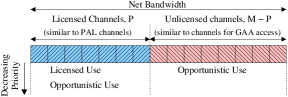
Figure 1: Pictorial representation of the tiered spectrum model under consideration in this paper.

There are various factors that decide the optimal values of $M$ and $P$. Some of these factors are as follows. If the number of channels $M$ increases, the bandwidth, and hence capacity, of each channel decreases. The capacity of each channel should be large enough to accommodate a good portion of the customer demand of a wireless operator but not so large that most of the capacity of the channel is not utilized for majority of the time. This suggests that $M$ should not be too small or too large. If the number of licensed channels $P$ is too high, there is a small number of unlicensed channels. Therefore, those operators who primarily rely on unlicensed channels to serve customer demands will not be able to generate enough revenue and hence will not be incentivized to join the market. Similarly, if the $P$ is too low, wireless operators who primarily rely on licensed channels to serve customer demands will not be incentivized to join the market. $P$ should be set such that enough operators join the market to ensure that the customer demands served over the entire bandwidth is as high as possible. There may be other qualitative factors governing optimal $M$ and $P$. Therefore, in this paper, we design an algorithm to jointly optimize $M$ and $P$ such that spectrum utilization is maximized.

I-A Related Work

Variations of the spectrum partitioning and spectrum licensing problems considered in this paper have been studied separately, but not jointly, in the spectrum sharing and related fields. There are a few works that have addressed problems similar to partitioning of a fixed bandwidth into optimal number of channels. In [4], the authors derive an analytical expression for the optimal number of channels such that the spatial density of transmission is maximized subject to a fixed link transmission rate and packet error rate. Partitioning of bandwidth in the presence of guard bands has been considered in [5] where the authors used Stackelberg game formulation to analyze how a spectrum holder should partition its bandwidth in order to maximize its revenue in spectrum auctions.

The second problem studied in this paper essentially deals with spectrum licensing. This has been widely studied in the literature from various perspectives. Some works concentrated on minimizing the amount of bandwidth allocated to backup channels (unlicensed channels in our case) while providing a certain level of guarantee to secondary users against channel preemption [6]. There has also been research on overlay D2D and cellular devices which studied optimal partitioning of orthogonal in-band spectrum to maximize the average throughout rates of cellular and D2D devices [7]. In [8], the authors investigated whether to allocate an additional spectrum band for licensed or unlicensed use and concluded that the licensed use is more favourable for maximizing the social surplus. A similar result has been shown in [9] which studied the effect of adding an unlicensed spectrum band in a market consisting of wireless operators with licensed channels. The authors showed that if the amount of unlicensed spectrum band is below a certain limit, the the overall social welfare may decrease with the increase in unlicensed spectrum band. The authors in [10, 11] studied the CBRS band for a market setup that consists of Environmental Sensing Capability operators (ESCs) whose sole job is to monitor and report spectrum occupancy to the wireless operators. The authors analyzed how the ratio of the licensed and unlicensed bands affects the market competition between the ESC operators, the wireless operators, and the end users of the CBRS band. There is a line of work which studies spectrum partitioning for topics similar to licensed and unlicensed use using Stackelberg games; macro cells and small cells [12, 13], long-term leasing market and short-term rental market [14], and 4G cellular and Super Wifi services [15].

Such a diverse body of work just on spectrum partitioning and licensing is justified because individual problem setups have their own salient features and hence require their own analysis. Our problem setup considers jointly optimizing spectrum partitioning and spectrum licensing, which has not been considered in the existing literature. This problem is novel because of the combination of the following two reasons. First, our spectrum access model, like CBRS, is a combination of (a) Unlicensed spectrum access model. This is because $M-P$ unlicensed channels are reserved specifically for opportunistic use. (b) Primary-secondary spectrum access model. This is because $P$ licensed channels can be used for opportunistic access following the priority hierarchy. Prior works like [9, 10, 11], which solved the spectrum licensing problem, did not simultaneously consider both of the spectrum access models. Second, we consider a very generalized system model in terms of the number of operators, their types, and their heterogeneity. Such a setup leads to a scenario where the regulator has to decide $M$ and $P$ such that the right set of wireless operators are incentivized to join the market.

I-B Contribution and Paper Organization

We now present an overall outline of the paper and, in the process, discuss its main contributions. In Section II, we present a system model which can mathematically capture the effect of the number of channels, $M$, and number of licensed channels, $P$, on the spectrum utilization. The proposed system model captures spectrum auctions using a simple stochastic model without going into complex game-theoretic formulations. Based on our reading of [1, 2, 3] and other literature on CBRS band, it is not clear if there is a consensus in the literature/policy about whether PAL license holders are also allowed to use channels opportunistically. So it is possible that PAL license holders may or may not be allowed to use channels opportunistically. Our model is general enough to capture both of these cases. Our model also generalizes well to various opportunistic access strategies like overlay or interweave spectrum access [16].

It is possible that a choice of values of $M$ and $P$ that incentivizes one group of wireless operators may not incentivize another group. Therefore, a $M$ and $P$ which incentivizes all the wireless operators may not exist. This argument can be exemplified by refering to [1, 2, 3] which shows a lot of debate between the wireless operators concerning the parameters of the CBRS model. Even if it is possible to satisfy all the operators, it may not be optimal to do so in terms of maximizing the spectrum utilization. We capture this idea by formulating our problem as a two-stage Stackelberg game in Section III-A which forms the second contribution of the paper. The Stackelberg game consists of the regulator (leader) and the wireless operators (followers). In Stage 1, the regulator sets $M$ and $P$ to maximize spectrum utilization. In Stage 2, the wireless operators decide whether or not to join the market based on the $M$ and $P$ set by the regulator in Stage 1.

In Section III-B, we design an algorithm to solve the Stackelberg game and hence the optimal $M$ and $P$ which maximize spectrum utilization. We approach this in steps. Few properties associated with expected revenue of an operator are discussed first. We show that when these properties hold, we can design a polynomial time algorithm to solve Stage 2 of the Stackelberg game. We finally solve Stage 1 of the Stackelberg game using a grid search approach to find the optimal $M$ and $P$ which maximizes spectrum utilization. To the best of our knowledge, joint optimization of partitioning and tiered licensing have not been considered in the existing related literature. Hence, designing an algorithm for joint optimization of $M$ and $P$ is the fourth contribution of the paper.

The solve the Stackelberg game, we have to calculate the expected revenue of an operator and expected spectrum utilization. The complex nature of the problem does not allow simple analytical formulas of these expected values. Even if such analytical formulas are possible, adapting them to changes in system model can be time consuming. Therefore, we develop a Monte Carlo integrator to evaluate these expected values in Section IV. Our choice of using a Monte Carlo integrator over deterministic numerical integration techniques is because our setup involves evaluation of high-dimensional integrals. Unlike deterministic numerical integration techniques, the computation time of Monte carlo integration does not scale with dimension. One of the main bottlenecks of Monte Carlo integration is random sampling. While designing our Monte Carlo integrator, we reduced random sampling as much as possible to make it more time efficient. Designing an efficient Monte Carlo integrator which can easily adapt to few changes in the system model is the third contribution of the paper.

Finally, we use the algorithms designed in Sections III-B and IV to obtain important numerical results in Section V which constitutes the final contribution of the paper. Our numerical results show how optimal values of $M$ and $P$ vary with market parameters.

II System Model

In this section, we discuss individual components of our system model in Sections II-A to II-C. The list of important notations is included in Table I. We introduce three set theoretic notations. Consider two sets $\mathcal{A}$ and $\mathcal{B}$. The operation $\mathcal{A}\bigcup\mathcal{B}$ implies the union $\mathcal{A}$ and $\mathcal{B}$. The operation $\mathcal{A}\backslash\mathcal{B}$ is as set which consists of all those elements in $\mathcal{A}$ which are not in $\mathcal{B}$. A singleton set consisting of element $a$ is denoted by $\left\{a\right\}$.

Table I: A table of important notations.

Notation	Description
$t$ , $\gamma$	$t^{th}$ time slot and epoch $\gamma$ resp.
$M$ , $P$	Number of channels and number of licensed channels resp.
$\phi$	Indicator variable which decides if a Tier-1 operator can also use channels opportunistically. We have, $\phi\in\left\{0,1\right\}$.
$D$	Capacity of the entire bandwidth for licensed access.
$\alpha_{L}$ , $\alpha_{U}$	Interference parameter associated with opportunistic use of licensed and unlicensed channels resp.
$\mathcal{S}_{L}^{C}$ , $\mathcal{S}_{U}^{C}$	Set of candidate licensed and unlicensed operators resp.
$\mathcal{S}_{L}$ , $\mathcal{S}_{U}$	Set of interested licensed and unlicensed operators resp.
$\mathcal{S}$	Set of interested operators; $\mathcal{S}=\mathcal{S}_{L}\bigcup\mathcal{S}_{U}$.
$\mathcal{T}_{1}\left(\gamma\right)$	Set of Tier-1 operators in epoch $\gamma$, i.e. set of interested licensed operators who won licensed channels in epoch $\gamma$.
$\mathcal{T}_{2}\left(\gamma\right)$	Set of Tier-2 operators in epoch $\gamma$; $\mathcal{T}_{2}\left(\gamma\right)=\mathcal{S}\backslash\mathcal{T}_{1}\left(\gamma\right)$.
$x_{k}\left(t\right)$	Customer demand of the $k^{th}$ operator in $t^{th}$ time slot.
$\mu_{k}^{\theta}$ , $\sigma_{k}^{\theta}$	Mean and standard deviation resp. of Gaussian random variable $\theta_{k}\left(t\right)$ where, $x_{k}\left(t\right)=\max\left(0,\theta_{k}\left(t\right)\right)$.
$\widetilde{x}_{k,i}\left(t\right)$	Amount of demand served by the $k^{th}$ operator in $t^{th}$ time slot if it is a Tier-$i$ operator where $i\in\left\{1,2\right\}$.
$\widetilde{x}_{k,a}\left(t\right)$	Amount of demand served by the $k^{th}$ operator in $t^{th}$ time slot when spectrum access type is $a$ where $a\in\left\{lc,op\right\}$.
$X_{k,a}\left(\gamma\right)$	Net demand served by the $k^{th}$ operator in epoch $\gamma$ when spectrum access type is $a$ where $a\in\left\{lc,op\right\}$.
$R_{k,a}\left(\gamma\right)$	Revenue of $k^{th}$ operator in epoch $\gamma$ using spectrum access of type $a$ where $a\in\left\{lc,op\right\}$.
$R_{k,i}\left(\gamma\right)$	Revenue of $k^{th}$ operator in epoch $\gamma$ if it is a Tier-$i$ operator.
$V_{k}\left(\gamma\right)$	Bid of the $k^{th}$ operator, where $k\in\mathcal{S}_{L}$, in epoch $\gamma$.
$h_{k}\left(\cdot\right)$	A function associated with $k^{th}$ operator which maps the mean of $X_{k,a}\left(\gamma\right)$ to the mean of $R_{k,a}\left(\gamma\right)$.
$\mu_{k,a}^{X}\,,\,\sigma_{k,a}^{X}$	Mean and standard deviation of $X_{k,a}\left(\gamma\right)$.
$\mu_{k,a}^{R}\,,\,\sigma_{k,a}^{R}$	Mean and standard deviation of $R_{k,a}\left(\gamma\right)$. We have, $\mu_{k,a}^{R}$=$h_{k}\left(\mu_{k,a}^{X}\right)$.
$\rho_{k}$	Correlation coefficent between $X_{k,a}\left(\gamma\right)$ and $R_{k,a}\left(\gamma\right)$.
$\omega_{k}$	Correlation coefficent between $V_{k}\left(\gamma\right)$ and $R_{k,lc}\left(\gamma\right)$.
$\lambda_{k}$	Minimum revenue requirement of the $k^{th}$ operator.
$\xi_{k}$	The tuple $\left(\mu_{k}^{\theta},\,\sigma_{k}^{\theta},\,h_{k}\left(\cdot\right),\,\sigma_{k,a}^{R},\,\rho_{k},\,\rho_{k},\,\lambda_{k}\right)$ associated with the $k^{th}$ operator.
$\left(x\right)^{+}$	$\left(x\right)^{+}=\max\left(0,x\right)$

II-A Channel Model

A net bandwidth of $W\>hz$ is divided into $M$ channels of equal bandwidth $\frac{W}{M}$. Out of the $M$ channels, $P$ channels are licensed channels while the remaining $M-P$ channels are unlicensed channels. In our model, time is divided into slots where $t\in\mathbb{Z}^{+}$ denotes the $t^{th}$ time slot. Licensed channels are allocated for prioritized licensed use and opportunistic use while unlicensed channels are allocated only for opportunistic use. Allocation of licensed channels for licensed use happens through auctions. These auctions occur every $T\geq$1 time slots where $T$ is the lease duration. An entire lease duration is called an “epoch”. Epoch $\gamma$ is from time slot $\left(\gamma-1\right)T+1$ to $\gamma T$. Allocation of licensed channels and unlicensed channels for opportunistic use occur every time slot.

Those operators who are allocated licensed channels for licensed use are called Tier-1 operators while those who are not are called Tier-2 operators. In our model, an operator can be allocated atmost one licensed channel for licensed use in an epoch, i.e. spectrum cap is one. Similar assumptions has been made in prior works like [17]. Spectrum cap of one ensures fairness by allocating the licensed channels to as many operators as possible. A Tier-1 operator can also use opportunistic channels to serve its customer demand in case the bandwidth of the allocated licensed channel is not sufficient. Tier-2 operators uses channels opportunsitically. Tier-1 operators may also use channels opportunistically. Let $\phi\in\left\{0,1\right\}$ be an indicator variable which decides if Tier-1 operators can use channels opportunistically. If $\phi=1$, then Tier-1 operators can use channels opportunistically and otherwise they cannot.

The capacity of a channel/bandwidth is the maximum units of customer demand that can be served using that channel/bandwidth in a time slot. Let $D$ be the capacity of the entire bandwidth of $W\>hz$ when used for licensed access. As the entire bandwidth is partitioned into $M$ channels, each licensed channel has a capacity of $\frac{D}{M}$ when used for licensed use while the unlicensed channels has a capacity of $\frac{\alpha_{U}D}{M}$ where $\alpha_{U}\in\left[0,1\right]$ is the interference parameter associated with unlicensed channels for opportunistic use. Licensed channels can also be used for opportunistic use following the priority hierarchy shown in Figure 1. Let the customer demand of a Tier-1 operator be $d$ units. It will use its licensed channel to serve its customer demand. The remaining capacity of the licensed channel which can be utilized for opportunsitic use is given by the function $\mathcal{C}\left(d,\alpha_{L}\right)$ where $\alpha_{L}\in\left[0,1\right]$ is the interference parameter associated with licensed channels for opportunistic use. The expression for $\mathcal{C}\left(d,\alpha_{L}\right)$ depends on the opportunistic spectrum access (OSA) strategy: overlay or interweave [16]. For overlay spectrum access, $\mathcal{C}\left(d,\alpha_{L}\right)=\alpha_{L}\left(\frac{D}{M}-d\right)^{+}$, where $\left(x\right)^{+}=\max\left(0,x\right)$. For interweave spectrum access, $\mathcal{C}\left(d,\alpha_{L}\right)$ is equal to $0$ if $d>0$ and equal to $\frac{\alpha_{L}D}{M}$ if $d=0$. Parameters $\alpha_{L}$ and $\alpha_{U}$ capture the lower efficiency of opportunistic use as compared to licensed use [1]. In general, we expect $\alpha_{L}\leq\alpha_{U}$. This may happen because the transmission power cap for opportunistic use maybe lower for licensed channels compared to unlicensed channels in order to protect Tier-1 operators from harmful interference.

II-B Operators, their Demand and Revenue Model

The market consists of the candidate licensed operators denoted by $\mathcal{S}_{L}^{C}$ and the candidate unlicensed operators denoted by $\mathcal{S}_{U}^{C}$ where $\mathcal{S}_{L}^{C}$ and $\mathcal{S}_{U}^{C}$ are disjoint sets. A candidate licensed operator is a Tier-1 operator in those epochs in which it is allocated a licensed channel in the auction and a Tier-2 operator in those epochs in which it is not allocated a licensed channel. A candidate unlicensed operator is always a Tier-2 operator. A candidate operator has to invest in infrastructure development if it wants to join the market.

All the candidate operators have to invest in infrastructure development to join the market. In order to generate return on infrastructure cost and the cost of leasing a channel, a candidate operator wants to earn a minimum expected revenue in an epoch. Let $\lambda_{k}$ be the minimum expected revenue (MER) of the $k^{th}$ operator. A subset of candidate licensed and unlicensed operators are interested in joining the market if the value of $M$ and $P$ set by the regulator is such that the expected revenue of the operator in an epoch is greater than its MER. The set of interested licensed operators and interested unlicensed operators are denoted by $\mathcal{S}_{L}$ and $\mathcal{S}_{U}$ respectively. We have $\mathcal{S}_{L}\subseteq\mathcal{S}_{L}^{C}$ and $\mathcal{S}_{U}\subseteq\mathcal{S}_{U}^{C}$. The set of operators, $\left(\mathcal{S}_{L}^{C}-\mathcal{S}_{L}\right)\bigcup\left(\mathcal{S}_{U}^{C}-\mathcal{S}_{U}\right)$, does not join the market. A candidate licensed/unlicensed operator gets to decide whether to join or not join the market only once. An operator gets to participate in auctions for licensed channels or to use channels opportunistically only if it decides join the market.

In our model, every operator has a separate pool of customers each with its own stochastic demands, i.e. we do not model price competition between operators to attract a common pool of customers. Consider the $t^{th}$ time slot of epoch $\gamma$. The customer demand, or simply demand, of the $k^{th}$ operator in the $t^{th}$ time slot is $x_{k}\left(t\right)$. In our model, $x_{k}\left(t\right)=\max\left(0\,,\,\theta_{k}\left(t\right)\right)$ where $\theta_{k}\left(t\right)$ are iid Gaussian random variable with mean $\mu_{k}^{\theta}$ and standard deviation $\sigma_{k}^{\theta}$, i.e. $\theta_{k}\left(t\right)\sim\mathcal{N}\left(\mu_{k}^{\theta},\left(\sigma_{k}^{\theta}\right)^{2}\right)\,,\,\forall t$. The $k^{th}$ operator may be able to serve only a fraction of the customer demand. Let $\widetilde{x}_{k,1}\left(t\right)$ and $\widetilde{x}_{k,2}\left(t\right)$ denote the amount of customer demand served by the $k^{th}$ operator if it is a Tier-1 and a Tier-2 operator respectively in epoch $\gamma$. We have $\widetilde{x}_{k,1}\left(t\right)\leq x_{k}\left(t\right)$ and $\widetilde{x}_{k,2}\left(t\right)\leq x_{k}\left(t\right)$. $\widetilde{x}_{k,1}\left(t\right)$ and $\widetilde{x}_{k,2}\left(t\right)$ can be expressed as follows

$$\widetilde{x}_{k,1}\left(t\right) = \widetilde{x}_{k,lc}\left(t\right)+\widetilde{x}_{k,op}\left(t\right)$$ (1)

$$\widetilde{x}_{k,2}\left(t\right) = \widetilde{x}_{k,op}\left(t\right)$$ (2)

where $\widetilde{x}_{k,lc}\left(t\right)=\min\left(x_{k}\left(t\right),\frac{D}{M}\right)$. The term $\widetilde{x}_{k,lc}\left(t\right)$ in (1) is the amount of customer demand served a Tier-1 operator using the channel allocated to it for licensed use. The term $\widetilde{x}_{k,op}\left(t\right)$ in (1) and (2) is the demand served by an operator by using channels opportunistically. It will be shown in Section II-C that $\widetilde{x}_{k,op}\left(t\right)$ is a iid random variable. Also, if $\phi=0$, then a Tier-1 operator cannot use channels opportunistically and hence $\widetilde{x}_{k,op}\left(t\right)\equiv 0$ in (1). In (1) and (2), $\widetilde{x}_{k,1}\left(t\right)$ and $\widetilde{x}_{k,2}\left(t\right)$ can be expressed as a time invariant function of iid random variables $x_{k}\left(t\right)$ and $\widetilde{x}_{k,op}\left(t\right)$. Therefore, $\widetilde{x}_{k,1}\left(t\right)$ and $\widetilde{x}_{k,2}\left(t\right)$ are iid random variables as well. Let $\widetilde{\mu}_{k,a}^{x}$ and $\widetilde{\sigma}_{k,a}^{x}$ denote the mean and standard deviation of $\widetilde{x}_{k,a}\left(t\right)$ respectively. We have,

$$\widetilde{\mu}_{k,lc}^{x}=\stackrel{{\scriptstyle[}}{{0}}]{\frac{D}{M}}{\int}\vartheta f_{k}^{\theta}\left(\vartheta\right)\,d\vartheta+\frac{D}{M}\stackrel{{\scriptstyle[}}{{\frac{}}{missing}}{D}{M}]{\infty}{\int}f_{k}^{\theta}\left(\vartheta\right)\,d\vartheta$$ (3)

$$\left(\widetilde{\sigma}_{k,lc}^{x}\right)^{2}=\stackrel{{\scriptstyle[}}{{0}}]{\frac{D}{M}}{\int}\vartheta^{2}f_{k}^{\theta}\left(\vartheta\right)\,d\vartheta+\left(\frac{D}{M}\right)^{2}\stackrel{{\scriptstyle[}}{{\frac{}}{missing}}{D}{M}]{\infty}{\int}f_{k}^{\theta}\left(\vartheta\right)\,d\vartheta-\left(\widetilde{\mu}_{k,lc}^{x}\right)^{2}$$ (4)

where $f_{k}^{\theta}\left(\vartheta\right)$ is the probability density function of $\theta_{k}\left(t\right)$. In general, an analytical expression for $\widetilde{\mu}_{k,op}^{x}$ and $\widetilde{\sigma}_{k,op}^{x}$ is not possible because of the complex nature of opportunistic spectrum allocation algorithm. We have designed a Monte Carlo integrator which can compute $\widetilde{\mu}_{k,op}^{x}$ in Section IV.

Throughout the rest of the paper we will use the subscript $k,i$, where $i\in\left\{1,2\right\}$, to denote variables associated with $k^{th}$ operator when its is a Tier-$i$ operator. Also, we will use the subscript $k,a$, where $a\in\left\{lc,op\right\}$, to denote variables associated with $k^{th}$ operator when access type is licensed ($a=lc$) or opportunistic ($a=op$). Let $X_{k,a}\left(\gamma\right)$ denote the net demand served by the $k^{th}$ operator in epoch $\gamma$ when access type is $a$. Mathematically,

$$X_{k,a}\left(\gamma\right)=\stackrel{{\scriptstyle[}}{{t}}=\left(\gamma-1\right)T+1]{\gamma T}{\sum}\widetilde{x}_{k,a}\left(t\right)\;;\>a\in\left\{lc,op\right\}$$ (5)

Since $\widetilde{x}_{k,a}\left(t\right)$ is iid random variable and the lease duration $T$ is quite large in practice, $X_{k,a}\left(\gamma\right)$ can be approximated as a Gaussian random variable using Central Limit Theorem [18, Chapter 8]. The mean, $\mu_{k,a}^{X}$, and standard deviation, $\sigma_{k,a}^{X}$, of $X_{k,a}\left(\gamma\right)$ are given by

$$\mu_{k,a}^{X}=\widetilde{\mu}_{k,a}^{x}T\qquad;\qquad\sigma_{k,a}^{X}=\widetilde{\sigma}_{k,a}^{x}\sqrt{T}$$ (6)

To this end we have, $X_{k,a}\left(\gamma\right)\sim\mathcal{N}\left(\mu_{k,a}^{X},\left(\sigma_{k,a}^{X}\right)^{2}\right)\,,\,\forall\gamma$.

Remark 1: Gaussian nature of $X_{k,a}\left(\gamma\right)$. $X_{k,a}\left(\gamma\right)$ is always a positive quantity because net demand served is always positive. But, we approximated $X_{k,a}\left(\gamma\right)$ as a Gaussian random variable and hence the approximated $X_{k,a}\left(\gamma\right)$ can be negative. However, the probability of $X_{k,a}\left(\gamma\right)$ being negative is

$$P\left[X_{k,a}\left(\gamma\right)<0\right]=\frac{1}{2}\left(1+\text{erf}\left(-\frac{\widetilde{\mu}_{k,a}^{x}\sqrt{T}}{\sqrt{2}\widetilde{\sigma}_{k,a}^{x}}\right)\right)$$

where $\text{erf}\left(\cdot\right)$ is the error function. For all practical setup, $T$ is large enough that $P\left[X_{k,a}\left(\gamma\right)<0\right]$ is very small. The use of Gaussian model for non-negative random variables have been used in prior works like [19].

An operator generates revenue by serving customer demand. Let $R_{k,a}\left(\gamma\right)$ denote the revenue earned by the $k^{th}$ operator in epoch $\gamma$ when access type is $a$. We model $R_{k,a}\left(\gamma\right)$ as a random variable which follows the stochastic model

$$\begin{bmatrix}X_{k,a}\left(\gamma\right)\\ R_{k,a}\left(\gamma\right)\end{bmatrix}\sim\mathcal{N}\left(\begin{bmatrix}\mu_{k,a}^{X}\\ \mu_{k,a}^{R}\end{bmatrix},\begin{bmatrix}\left(\sigma_{k,a}^{X}\right)^{2}&\rho_{k}\sigma_{k,a}^{X}\sigma_{k,a}^{R}\\ \rho_{k}\sigma_{k,a}^{X}\sigma_{k,a}^{R}&\left(\sigma_{k,a}^{R}\right)^{2}\end{bmatrix}\right)$$ (7)

for all $\gamma$ where $\mu_{k,a}^{R}=h_{k}\left(\mu_{k,a}^{X}\right)$. According to (7), the net demand served and the net revenue earned in epoch $\gamma$ are jointly Gaussian. The mean of $R_{k,a}\left(\gamma\right)$ is $\mu_{k,a}^{R}=h_{k}\left(\mu_{k,a}^{X}\right)$ where $h_{k}\left(\mu_{k,a}^{X}\right)$ is a monotonic increasing function of the mean demand served by the $k^{th}$ operator in an epoch, $\mu_{k,a}^{X}$. The standard deviation of $R_{k,a}\left(\gamma\right)$ is $\sigma_{k,a}^{R}$ which can be used to capture the effect of exogeneous stochastic processes like market dynamics on $R_{k,a}\left(\gamma\right)$. The relative change between $R_{k,a}\left(\gamma\right)$ and $X_{k,a}\left(\gamma\right)$ is captured with correlation coefficent $\rho_{k}\in\left[0,1\right)$. It captures how much a deviation of $X_{k,a}\left(\gamma\right)$ around its mean $\mu_{k,a}^{X}$ will effect the deviation of $R_{k,a}\left(\gamma\right)$ around its mean $h_{k}\left(\mu_{k,a}^{X}\right)$. A monotonic increasing function, $h_{k}\left(\cdot\right)$, and a positive correlation coefficient, $\rho_{k}$, are intuitive because from a statistical standpoint it implies that an operator who serves more customer demand generates higher revenue.

Let $R_{k,i}\left(\gamma\right)$ denote the revenue earned by the $k^{th}$ operator if it is a Tier-$i$ operator in epoch $\gamma$. Tier-1 serves customer demand using both licensed and opportunistic access while Tier-2 operator serves its customer demand using opportunistic access only. Hence,

$$R_{k,1}\left(\gamma\right) = R_{k,lc}\left(\gamma\right)+R_{k,op}\left(\gamma\right)$$ (8)

$$R_{k,2}\left(\gamma\right) = R_{k,op}\left(\gamma\right)$$ (9)

Notice that since $R_{k,lc}\left(\gamma\right)$ and $R_{k,op}\left(\gamma\right)$ are Gaussian, $R_{k,1}\left(\gamma\right)$ and $R_{k,2}\left(\gamma\right)$ are Gaussian as well.

II-C Spectrum Allocation Model

Licensed channels are allocated to the set of interested licensed osperators, $\mathcal{S}_{L}$, through spectrum auctions. The auction for epoch $\gamma$ happens at time slot $\left(\gamma-1\right)T+1$. The set of interested licensed operators bids for licensed channels. Let $V_{k}\left(\gamma\right)$ be the bid of the $k^{th}$ operator in epoch $\gamma$. Intuitively, the bid of the $k^{th}$ operator should depend on its valuation of a licensed channel. The value of a licensed channel to the $k^{th}$ operator in epoch $\gamma$ is $R_{k,lc}\left(\gamma\right)$, the revenue it can generate in an epoch using the licensed channel. We capture this dependence between $V_{k}\left(\gamma\right)$ and $R_{k,lc}\left(\gamma\right)$ using a correlation coefficient $\omega_{k}\in\left[0,1\right)$ between them. In our model, $V_{k}\left(\gamma\right)$ and $R_{k,lc}\left(\gamma\right)$ are jointly Gaussian. We have,

$$\begin{bmatrix}V_{k}\left(\gamma\right)\\ R_{k,lc}\left(\gamma\right)\end{bmatrix}\sim\mathcal{N}\left(\begin{bmatrix}\mu_{k,lc}^{R}\\ \mu_{k,lc}^{R}\end{bmatrix},\begin{bmatrix}\left(\sigma_{k,lc}^{R}\right)^{2}&\omega{}_{k}\left(\sigma_{k,lc}^{R}\right)^{2}\\ \omega{}_{k}\left(\sigma_{k,lc}^{R}\right)^{2}&\left(\sigma_{k,lc}^{R}\right)^{2}\end{bmatrix}\right)$$ (10)

for all $\gamma$. In (10), $\mu_{k,lc}^{R}=h_{k}\left(\widetilde{\mu}_{k,lc}^{x}T\right)$ (refer to (6) and (7)). Using a stochastic model like (10) to capture the relation between $V_{k}\left(\gamma\right)$ and $R_{k,lc}\left(\gamma\right)$ leads to a more generic system model because we can abstract away from the exact bid estimation strategies of the operators which may rely on various market externalities.

Given that there are $P$ licensed channels and the spectrum cap is one, the interested licensed operators with the $P$ highest bids $V_{k}\left(\gamma\right)$ are allocated one licensed channel each in epoch $\gamma$. The operators who are allocated a licensed channel have to pay a price that is determined by the regulator. Such a pricing model has been used in prior works [15]. Let $\mathcal{T}_{1}\left(\gamma\right)\subseteq\mathcal{S}_{L}$ denote the set of interested licensed operators who are allocated licensed channels in epoch $\gamma$. Similarly, $\overline{\mathcal{T}}_{1}\left(\gamma\right)=\mathcal{S}_{L}\backslash\mathcal{T}_{1}\left(\gamma\right)$ are the set of interested licensed operators who are not allocated licensed channels in epoch $\gamma$. The operators in $\mathcal{T}_{1}\left(\gamma\right)$ serve their customer demand as Tier-1 operators in epoch $\gamma$. On the other hand, operators in $\overline{\mathcal{T}}_{1}\left(\gamma\right)$ serve their customer demand as Tier-2 operators in epoch $\gamma$. It is to be noted that $\mathcal{T}_{1}\left(\gamma\right)$ and $\overline{\mathcal{T}}_{1}\left(\gamma\right)$ are random sets as they get decided by the bids $V_{k}\left(\gamma\right)$ which are random variables. The set of Tier-2 operators in epoch $\gamma$ is $\mathcal{T}_{2}\left(\gamma\right)=\overline{\mathcal{T}_{1}}\left(\gamma\right)\bigcup\mathcal{S}_{U}$, i.e., interested unlicensed operators and interested licensed operators who are not allocated a licensed channel in epoch $\gamma$. Unlike the sets $\mathcal{S}_{L}$ and $\mathcal{S}_{U}$ which are decided once, sets $\mathcal{T}_{1}\left(\gamma\right)$, $\overline{\mathcal{T}}_{1}\left(\gamma\right)$, and $\mathcal{T}_{2}\left(\gamma\right)$ are decided in the beginning of every epoch. A pictorial representation of all the important sets discussed till now is shown in Figure 2. Figure 2 also shows $\mathcal{T}_{1}\left(\gamma\right)$, $\overline{\mathcal{T}}_{1}\left(\gamma\right)$, and $\mathcal{T}_{2}\left(\gamma\right)$ varies with epoch $\gamma$.

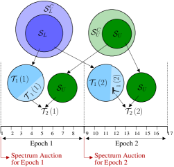
Figure 2: Pictorial representation of the set of candiate licensed operators $\mathcal{S}_{L}^{C}$, candiate unlicensed operators $\mathcal{S}_{U}^{C}$, interested licensed operators $\mathcal{S}_{L}$, interested unlicensed operators $\mathcal{S}_{U}$, the set of interested licensed operators who are allocated (not allocated) licensed channels in an epoch $\mathcal{T}_{1}\left(\gamma\right)$ ($\overline{\mathcal{T}}_{1}\left(\gamma\right)$) and the set of Tier-2 operators in an epoch $\mathcal{T}_{2}\left(\gamma\right)$. Note that $\mathcal{T}_{1}\left(\gamma\right)$, $\overline{\mathcal{T}}_{1}\left(\gamma\right)$ and $\mathcal{T}_{2}\left(\gamma\right)$ are not same for epochs $1$ and $2$.

Opportunistic spectrum allocation happens in every time slot to all the Tier-2 operators. Tier-1 operators may or may not participate in opportunistic spectrum access depending on whether $\phi$ is one or zero. In order to capture both these cases under a single mathematical abstraction, we modify the demand of Tier-1 and Tier-2 operators. Let $\overline{x}_{k}\left(t\right)$ be the modified demand of the $k^{th}$ operator which needs to be served using OSA. For time slot $t$ of epoch $\gamma$,

$$\overline{x}_{k}\left(t\right)=\begin{cases}\phi\cdot\left(x_{k}\left(t\right)-\frac{D}{M}\right)^{+}&;\,k\in\mathcal{T}_{1}\left(\gamma\right)\\ x_{k}\left(t\right)&;\,k\in\mathcal{T}_{2}\left(\gamma\right)\end{cases}$$ (11)

According to (11), for a Tier-2 operator, its entire demand $x_{k}\left(t\right)$ needs to be served using OSA. For Tier-1 operators, the excess demand which could not be satisfied with licensed use is $\left(x_{k}\left(t\right)-\frac{D}{M}\right)^{+}$. If $\phi=1$, this excess demand has to served using OSA. If $\phi=0$, then $\overline{x}_{k}\left(t\right)=0$ for Tier-1 operators implying that they don’t participate in OSA.

Opportunistic channel capacity in time slot $t$ of epoch $\gamma$ is

$${\textstyle D_{O}\left(t\right)=\alpha_{U}\left(M-\widetilde{P}\right)\frac{D}{M}+\underset{k\in\mathcal{T}_{1}\left(\gamma\right)}{\sum}\mathcal{C}\left(x_{k}\left(t\right),\alpha_{L}\right)}$$ (12)

where $\widetilde{P}=\min\left(\left|\mathcal{S}_{L}\right|,P\right)$. In (12), the first term is the net channel capacity of unlicensed channels and the second term is the net remaining channel capacity of the licensed channels. The variable $\widetilde{P}$ is used to capture edge cases where the number of licensed channels is more than number of interested licensed operators. In such cases, the remaining $P-\left|\mathcal{S}_{L}\right|$ channels which are not allocated to licensed operators are used as unlicensed channels. The expression for $\mathcal{C}\left(x_{k}\left(t\right),\alpha_{L}\right)$ depends on the OSA strategy (overlay or interweave) and has been discussed in Section II-A. As our model is inspired by the CBRS band, we have to ensure that opportunistic spectrum allocation is fair [20]. One approach to ensure fair allocation and to avoid wastage of channel capacity is to use a max-min fair algorithm, like the famous Waterfilling algorithm. A detailed exposition of max-min fairness can be found in [21, 22]. In this section, we present the Waterfilling algorithm, explain its working with an example and qualitatively justify how it ensures fairness and avoids wastage of channel capacity. Waterfilling algorithm will be used for opportunistic channel allocation throughout this paper.

Algorithm 1 is the psuedocode of Waterfilling algorithm. Let $\mathcal{S}$ denote the set of interested operators, i.e. $\mathcal{S}=\mathcal{S}_{L}\bigcup\mathcal{S}_{C}$. The union of Tier-1 and Tier-2 operators, $\mathcal{T}_{1}\left(\gamma\right)\bigcup\mathcal{T}_{2}\left(\gamma\right)$, is equal to $\mathcal{S}$. The inputs to Algorithm 1 are the opportunistic channel capacity, $D_{O}\left(t\right)$, and the modified demands of all the interested operators, $\left\{\overline{x}_{k}\left(t\right)\right\}_{k\in\mathcal{S}}$. The output of Algorithm 1 is the opportunistic channel capacity allocated to all the interested operators, $\left\{\widetilde{x}_{k,op}\left(t\right)\right\}_{k\in\mathcal{S}}$. $\widetilde{x}_{k,op}\left(t\right)$ is also equal to the demand served by the operators using OSA. We use the following example to explain Algorithm 1: the set of interested operators is $\mathcal{S}=\left\{1,2,3,5,7\right\}$, their corresponding modified demand is $\left\{5,9,3,7,2\right\}$, and the opportunistic channel capacity $D_{O}\left(t\right)=17$. The example is shown in Figure 3.

1

2

Input: $D_{O}\left(t\right)$, $\left\{\overline{x}_{k}\left(t\right)\right\}_{k\in\mathcal{S}}$

3

Output: $\left\{\widetilde{x}_{k,op}\left(t\right)\right\}_{k\in\mathcal{S}}$

4

5Sort the list $\left\{\overline{x}_{k}\left(t\right)\right\}_{k\in\mathcal{S}}$ in ascending order of $\overline{x}_{k}\left(t\right)$. Let $\kappa\left(j\right)$ denote the operator index corresponding to the $j^{th}$ position of the sorted list.

6Set unused opportunistic channel capacity $C=D_{O}\left(t\right)$ and the remaining number of interested operators to allocate channel capacity $N_{S}=\left|\mathcal{S}\right|$.

7for $j\leftarrow 1$ to $\left|\mathcal{S}\right|$ do

8      Set $\widetilde{x}_{\kappa\left(j\right),op}\left(t\right)=\min\left(\overline{x}_{\kappa\left(j\right)}\left(t\right)\,,\,\frac{C}{N_{S}}\right)$.

9     Set $C=C-\widetilde{x}_{\kappa\left(j\right),op}\left(t\right)$ and $N_{S}=N_{S}-1$.

Algorithm 1 Waterfilling Algorithm for Opportunistic Channel Allocation

Waterfilling algorithm allocates channel capacity to the set of interested operators in ascending order of their modified demand (lines 1 and 3). The sorted list of modified demand is $\left\{2,3,5,7,9\right\}$ and the operator index $\kappa\left(j\right)$ corresponding to position $j=1,2,3,4,5$ of the sorted list is $7$, $3$, $1$, $5$, $2$ respectively. In line 2, unused opportunistic channel capacity $C=17$ and the remaining number of interested operators who needs to be allocated channel capacity $N_{S}=5$. Inside the for loop, the algorithm reserves equal portion of unused opportunistic channel capacity $C$ for the remaining $N_{S}$ interested operators. This is done in line 4 where a maximum channel capacity of $\frac{C}{N_{S}}$ is reserved for the $\kappa\left(j\right)^{th}$ operator. This step ensures fairness of Waterfilling algorithm. The channel capacity allocated to the $\kappa\left(j\right)^{th}$ operator is the minimum of its modified demand (the required channel capacity) and the maximum reserved channel capacity of $\frac{C}{N_{S}}$. Accordingly, $C$ and $N_{S}$ are updated in line 5. In our example, for $j=1$, $\widetilde{x}_{7,op}\left(t\right)=\min\left(2,\frac{17}{5}\right)=2$ and hence the updated $C=17-2=15$ and $N_{S}=4$. For $j=2$, $\widetilde{x}_{3,op}\left(t\right)=\min\left(3,\frac{15}{4}\right)=3$ and hence the updated $C=15-3=12$ and $N_{S}=3$. For $j=3$, $\widetilde{x}_{1,op}\left(t\right)=\min\left(5,\frac{12}{3}\right)=4$ and hence the updated $C=12-4=8$ and $N_{S}=2$. The loop continues and finally $\widetilde{x}_{5,op}\left(t\right)=\widetilde{x}_{2,op}\left(t\right)=4$. Waterfilling algorithm prevents wastage of channel capacity by allocating no more than required channel capacity in line 4. This ensures that the unused opportunistic channel capacity $C$ is as high as possible for the operators with higher customer demand.

We end this section by proving that the output $\widetilde{x}_{k,op}\left(t\right)$ of Algorithm 1 are iid random variables. By refering to (12) and (11), we can conclude that $D_{O}\left(t\right)$ and $\overline{x}_{k}\left(t\right)$, which forms the input to Algorithm 1, are the ouptuts of time invariant functions of iid random variables $x_{k}\left(t\right)$ and $V_{k}\left(\gamma\right)$ ($V_{k}\left(\gamma\right)$ decides the random set $\mathcal{T}_{1}\left(\gamma\right)$ in (12)). This implies that $D_{O}\left(t\right)$ and $\overline{x}_{k}\left(t\right)$ are iid random variables as well. Also note that except the inputs $D_{O}\left(t\right)$ and $\overline{x}_{k}\left(t\right)$, Algorithm 1 is not dependent on time $t$. Therefore, Algorithm 1 can be expressed as a time-invariant function of iid random variables $D_{O}\left(t\right)$ and $\overline{x}_{k}\left(t\right)$. This directly implies that the output $\widetilde{x}_{k,op}\left(t\right)$ of Algorithm 1 are iid random variables.

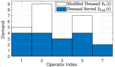
Figure 3: Pictorial representation of the example for Waterfilling algorithm.

Remark 2: Generality of the OSA model. We want to highlight that our OSA model is very general for three reasons. First, any opportunistic channel allocation algorithm can be used as long as $\widetilde{x}_{k,op}\left(t\right)$ are iid random variables. Second, the parameter $\phi$ helps us capture cases where Tier-1 operators can/cannot participate in OSA. Third, our model can capture both overlay and interweave OSA strategy.

III Optimization Problem

We start this section by formulating the optimization problem for joint spectrum partition as a two- stage Stackelberg Game in Section III-A. In the process of formulating the Stackelberg Game, we introduce two functions. First, is the revenue function of an operator which captures the expected revenue of an operator in an epoch. Second, is the objective function which is proportional to spectrum utilization of all the interested operators in the market. We then develop efficient algorithms to solve the two stages of the Stackelberg Game in Section III-B and hence find the optimal $M$ and $P$ which maximizes spectrum utilization. In sections III-A and III-B, we assume complete information games. This assumption leads to notational simplicity. Also, this assumption does not affect the technical contribution of the paper as the overall approach can be easily extended to incomplete information games. This is discussed in Section III-C.

III-A Stackelberg Game Formulation

In this section, we formulate the optimal spectrum partitioning problem as a two-stage Stackelberg game between the regulator and the wireless operators. The $k^{th}$ operator can be completely characterised by seven parameters which can be represented as a tuple $\xi_{k}=\left(\mu_{k}^{\theta},\,\sigma_{k}^{\theta},\,h_{k}\left(\cdot\right),\,\sigma_{k,a}^{R},\,\rho_{k},\,\omega_{k},\,\lambda_{k}\right)$. In sections III-A and III-B, we assume complete information games, i.e. an operator and the regulator knows $\xi_{k}$ of all the operators. The player in stage-1 of the Stackelberg game is the regulator whose decision variables are $M$ and $P$. The payoff of the regulator is the expected spectrum utilization over a period of $\Gamma\geq 1$ epochs which is given by

$${\textstyle{\displaystyle Q=}E\left[\stackrel{{\scriptstyle[}}{{\gamma}}=1]{\Gamma}{\sum}\;\stackrel{{\scriptstyle[}}{{t}}=\left(\gamma-1\right)T+1]{\gamma T}{\sum}\left(Q_{lc}\left(\gamma,t\right)+Q_{op}\left(\gamma,t\right)\right)\right]}\;\text{{where,}}$$ (13)

$$Q_{lc}\left(\gamma,t\right)=\underset{k\in\mathcal{T}_{1}\left(\gamma\right)}{{\textstyle\sum}}\widetilde{x}_{k,lc}\left(t\right)$$ (14)

$$Q_{op}\left(\gamma,t\right)=\underset{k\in\mathcal{S}}{{\textstyle\sum}}\widetilde{x}_{k,op}\left(t\right)$$ (15)

In (13), the inner summation is to calculate spectrum utilization over all time slots in an epoch while the outer summation is to calculate spectrum utilization over all the epochs. $Q_{lc}\left(\gamma,t\right)$ and $Q_{op}\left(\gamma,t\right)$ are the net spectrum utilization in time slot $t$ of epoch $\gamma$ by using licensed and opportunistic spectrum access respectively. The regulator wants to maximize $Q$. Using linearity of expectation, we can rewrite (13) as

$$Q=\stackrel{{\scriptstyle[}}{{\gamma}}=1]{\Gamma}{\sum}\;\stackrel{{\scriptstyle[}}{{t}}=\left(\gamma-1\right)T+1]{\gamma T}{\sum}E\left[Q_{lc}\left(\gamma,t\right)+Q_{op}\left(\gamma,t\right)\right]$$ (16)

We now prove that $E\left[Q_{lc}\left(\gamma,t\right)+Q_{op}\left(\gamma,t\right)\right]$ is not a function of $\gamma$ and $t$. Based on (14) and (15), $\widetilde{x}_{k,lc}\left(t\right)$, $\widetilde{x}_{k,op}\left(t\right)$, and $\mathcal{T}_{1}\left(\gamma\right)$ are the only random variables in the expressions of $Q_{lc}\left(\gamma,t\right)$ and $Q_{op}\left(\gamma,t\right)$. As discussed in previous sections, $\widetilde{x}_{k,lc}\left(t\right)$ and $\widetilde{x}_{k,op}\left(t\right)$ are iid random variables. $\mathcal{T}_{1}\left(\gamma\right)$ is a function of bids $V_{k}\left(\gamma\right)$ of the operators. Since, $V_{k}\left(\gamma\right)$ is an iid random variable, so is $\mathcal{T}_{1}\left(\gamma\right)$. This discussion implies that $Q_{lc}\left(\gamma,t\right)+Q_{op}\left(\gamma,t\right)$ itself is an iid random variable and hence its expectation is independent of $\gamma$ and $t$. Infact, it is a function of $M$, $P$, $\mathcal{S}_{L}$ and $\mathcal{S}_{U}$. Let,

$$U\left(M,P,\mathcal{S}_{L},\mathcal{S}_{U}\right)=E\left[Q_{lc}\left(\gamma,t\right)+Q_{op}\left(\gamma,t\right)\right]$$ (17)

Substituting (17) in (16) we get,

$$Q=\Gamma TU\left(M,P,\mathcal{S}_{L},\mathcal{S}_{U}\right)$$ (18)

Equation 18 shows that maximizing $Q$ is same as maximizing $U\left(M,P,\mathcal{S}_{L},\mathcal{S}_{U}\right)$. Therefore, we will use $U\left(M,P,\mathcal{S}_{L},\mathcal{S}_{U}\right)$ as the payoff function of the regulator in the rest of the paper. $U\left(M,P,\mathcal{S}_{L},\mathcal{S}_{U}\right)$ is also called the objective function as it is a direct measure of spectrum utilization which we are trying to maximize in this paper.

The players in stage-2 of the Stackelberg game are the candidate licensed operators, $\mathcal{S}_{L}^{C}$, and candidate unlicensed operators, $\mathcal{S}_{U}^{C}$. The decision variables of the Stage-2 game are the set of interested licensed operators, $\mathcal{S}_{L}$, and the set of interested unlicensed operators, $\mathcal{S}_{U}$. The $k^{th}$ operator is interested in joining the market only if the expected revenue in an epoch is greater than $\lambda_{k}$. The expected revenue in an epoch of an interested licensed or unlicensed operator is given by the revenue function. The formula for revenue function if different for interested licensed operators and interested unlicensed operators. The revenue function of an interested licensed operator, i.e. $k\in\mathcal{S}_{L}$, is

$$\mathcal{R}_{k}\left(M,P,\mathcal{S}_{L},\mathcal{S}_{U}\right)\quad\quad\quad\quad\quad\quad\quad\quad\quad\quad\quad\quad\quad\quad$$

$$=E\left[R_{k,1}\left(\gamma\right)\,|\,\mathcal{E}_{k}^{\gamma}\right]P\left[\mathcal{E}_{k}^{\gamma}\right]+E\left[R_{k,2}\left(\gamma\right)\,|\,\overline{\mathcal{E}_{k}^{\gamma}}\right]P\left[\overline{\mathcal{E}_{k}^{\gamma}}\right]$$ (19)

$$=E\left[R_{k,lc}\left(\gamma\right)\,|\,\mathcal{E}_{k}^{\gamma}\right]P\left[\mathcal{E}_{k}^{\gamma}\right]\quad\quad\quad\quad\quad\quad\quad\quad\quad\quad\quad\quad\quad$$

$$+E\left[R_{k,op}\left(\gamma\right)\,|\,\mathcal{E}_{k}^{\gamma}\right]P\left[\mathcal{E}_{k}^{\gamma}\right]+E\left[R_{k,op}\left(\gamma\right)\,|\,\overline{\mathcal{E}_{k}^{\gamma}}\right]P\left[\overline{\mathcal{E}_{k}^{\gamma}}\right]$$ (20)

$$=E\left[R_{k,lc}\left(\gamma\right)\,|\,\mathcal{E}_{k}^{\gamma}\right]P\left[\mathcal{E}_{k}^{\gamma}\right]+h_{k}\left(\mu_{k,op}^{X}\right)\quad\quad\quad\quad\quad\quad$$ (21)

where $P\left[Z\right]$ denotes the probability of event $Z$, $\mathcal{E}_{k}^{\gamma}$ ($\overline{\mathcal{E}_{k}^{\gamma}}$) is the event that $k\in\mathcal{T}_{1}\left(\gamma\right)$ ($k\in\mathcal{T}_{2}\left(\gamma\right)$). In (19), $E\left[R_{k,i}\left(\gamma\right)\,|\,\mathcal{E}_{k}^{\gamma}\right]$ is the expected revenue of the $k^{th}$ operator if it is a Tier-$i$ operator in epoch $\gamma$. Finally, (19) is obtained using the law of total expectation. Equation 20 is obtained by substituting $R_{k,1}\left(\gamma\right)=R_{k,lc}\left(\gamma\right)+R_{k,op}\left(\gamma\right)$ (refer to (8)). Equation 21 is obtained by noticing that the sum of the second and the third term of (20) is equal to $E\left[R_{k,op}\left(\gamma\right)\right]$ which in turn in equal to $h_{k}\left(\mu_{k,op}^{X}\right)$ according to (7). Similar to the objective function, the revenue function of an interested licensed operator is also not a function of epoch $\gamma$. This is because the statistical properties of the involved random variables $R_{k,1}\left(\gamma\right)$ and $R_{k,2}\left(\gamma\right)$ are independent of $\gamma$.

If the $k^{th}$ operator is an interested unlicensed operator, i.e. $k\in\mathcal{S}_{U}$, it is always a Tier-2 operator. Hence, its expected revenue in an epoch is

$$\mathcal{R}_{k}\left(M,P,\mathcal{S}_{L},\mathcal{S}_{U}\right)=E\left[R_{k,2}\left(\gamma\right)\right]=h_{k}\left(\mu_{k,op}^{X}\right)$$ (22)

where $E\left[R_{k,2}\left(\gamma\right)\right]=h_{k}\left(\mu_{k,op}^{X}\right)$ because $R_{k,2}\left(\gamma\right)=R_{k,op}\left(\gamma\right)$ (refer to (9)) and $E\left[R_{k,op}\left(\gamma\right)\right]=h_{k}\left(\mu_{k,op}^{X}\right)$.

Payoff function of an operator who is interested in joining the market either as a licensed or an unlicensed operator is

$$\pi_{k}\left(M,P,\mathcal{S}_{L},\mathcal{S}_{U}\right)=\mathcal{R}_{k}\left(M,P,\mathcal{S}_{L},\mathcal{S}_{U}\right)-\lambda_{k}$$ (23)

where $\mathcal{R}_{k}\left(M,P,\mathcal{S}_{L},\mathcal{S}_{U}\right)$ is given by (19) if $k\in\mathcal{S}_{L}$ and by (22) if $k\in\mathcal{S}_{U}$. If an operator does not join the market, its payoff is zero. An operator decides to enter the market only if its payoff $\pi_{k}\left(M,P,\mathcal{S}_{L},\mathcal{S}_{U}\right)$ is strictly greater than zero.

With (23) as the payoff function, Stage-2 game may have multiple Nash Equilibriums which complicates the analysis. This can be simplified if we assume that the operators are pessimistic in nature. By doing so, we can get an unique solution of the Stage-2 game. Pessimistic models to address the issue of multiple Nash Equilibriums have been considered in prior works like [23, 24, 25]. One simple approach to model pessimistic decision making strategy is to use the concept of dominant strategy, i.e. an operator decides to join the market if and only if joining the market is its optimal strategy irrespective of whether other operators decides to join the market. However, in this paper, we model a pessimistic operators’ decision making strategy using iterated elimination of strictly dominated strategies (IESDS) [26]. Compared to dominant strategy, IESDS is a less pessimistic decision making strategy because more operators will join the market.

IESDS can be explained as follows. IESDS consists of iterations. Consider the first iteration which is the original Stage-2 game. We iterate through all the candidate licensed and unlicensed operators to check if either joining the market or not joining the market is a dominant strategy for any of the operators. The operators whose dominant strategy is to join (not join) the market will join (not join) the market irrespective of other operators’ decisions. This reduces the size of the Stage-2 game as it effectively consist of those operators who could not decide whether to join (not join) the market in the first iteration. Such operators are called confused operators in this paper. These confused operators who did not have a dominant strategy in the original Stage-2 game may have a dominant strategy in the reduced Stage-2 game. Therefore, in the second iteration, we find the dominant strategy of the confused operators in the reduced Stage-2 game. Such iterations continue until convergence, which happens when the reduced Stage-2 game does not have any dominant strategy. It is possible that there are ’confused operators’ even after convergence. Those operators will not join the market because in our model, the operators are pessimistic in nature.

III-B Solution of the Stackelberg Game

In this subsection, we use the process of backward induction [27] to solve the Stackelberg Game formulated in Section III-A. To apply backward induction, we first solve Stage-2 of the game followed by Stage-1. The following properties of the revenue function (as given by (19) and (22)) are crucial in designing an efficient algorithm to solve Stage-2 of the Stackelberg Game.

Property 1.

$\mathcal{R}_{k}\left(M,P,\mathcal{S}_{L},\mathcal{S}_{U}\right)$ is monotonic decreasing in $\mathcal{S}_{L}$, i.e. $\mathcal{R}_{k}\left(M,P,\mathcal{S}_{L},\mathcal{S}_{U}\right)\geq\mathcal{R}_{k}\left(M,P,\mathcal{S}_{L}\bigcup\left\{a\right\},\mathcal{S}_{U}\right)$ where $a\notin\mathcal{S}_{L}$ and $a\in\mathcal{S}_{L}^{C}$.

Property 2.

$\mathcal{R}_{k}\left(M,P,\mathcal{S}_{L},\mathcal{S}_{U}\right)$ is monotonic decreasing in $\mathcal{S}_{U}$, i.e. $\mathcal{R}_{k}\left(M,P,\mathcal{S}_{L},\mathcal{S}_{U}\right)\geq\mathcal{R}_{k}\left(M,P,\mathcal{S}_{L},\mathcal{S}_{U}\bigcup\left\{a\right\}\right)$ where $a\notin\mathcal{S}_{U}$ and $a\in\mathcal{S}_{U}^{C}$.

We have verified these properties numerically using the Monte Carlo integrator which will described in Section IV. These properties can be justified as follows. Property 1 states that as the set of interested licensed operators, $\mathcal{S}_{L}$, increases, the revenue function of both the licensed and the unlicensed operators decreases. The revenue function of a licensed operator decreases with increase in $\mathcal{S}_{L}$ because the operator has to compete with more operators in the spectrum auctions to get a channel. This reduces the operator’s probability of winning spectrum auctions which in turn decreases its revenue function as it can effectively serve fewer customer demand. The revenue function of an unlicensed operator also decreases with increase in $\mathcal{S}_{L}$. This happens because with increase in $\mathcal{S}_{L}$, there is an increase in the number of operators interested in opportunistic channel access. This reduces the share of opportunistic channels for an unlicensed operator. Therefore, its revenue decreases as it can serve fewer customer demand. Property 2 states that as the set of interested unlicensed operators, $\mathcal{S}_{U}$, increases, the revenue function of both the licensed and the unlicensed operators decreases. This happens because with increase in $\mathcal{S}_{U}$, the share of opportunistic channel decreases for a licensed or an unlicensed operator. This in turn decreases its revenue function.

1

2

Input: $M$, $P$, $T$, $D$, $\alpha_{L}$, $\alpha_{U}$, $\mathcal{S}_{L}^{C}$, $\mathcal{S}_{U}^{C}$ and $\xi_{k};\forall k\in\mathcal{S}_{L}^{C}\bigcup\mathcal{S}_{U}^{C}$

3

Output: $\mathcal{S}_{L}\left(M,P\right)$ and $\mathcal{S}_{U}\left(M,P\right)$

4

5Set $\widehat{\mathcal{X}}_{0}=\emptyset$, $\widetilde{\mathcal{X}}_{0}=\mathcal{S}_{L}^{C}$, $\widehat{\mathcal{Y}}_{0}=\emptyset$ and $\widetilde{\mathcal{Y}}_{0}=\mathcal{S}_{U}^{C}$.

6

7Set $converged=False$ and $l=0$.

8

9while $not\left(converged\right)$ do

10    Set $converged=True$ and $l=l+1$.

11   

12   Set $\widehat{\mathcal{X}}_{l}=\widehat{\mathcal{X}}_{l-1}$, $\widetilde{\mathcal{X}}_{l}=\widetilde{\mathcal{X}}_{l-1}$, $\widehat{\mathcal{Y}}_{l}=\widehat{\mathcal{Y}}_{l-1}$ and $\widetilde{\mathcal{Y}}_{l}=\widetilde{\mathcal{Y}}_{l-1}$.

13   

14   for $k$ in $\widetilde{\mathcal{X}}_{l-1}$ do

15       if $\mathcal{R}_{k}\left(M,P,\widehat{\mathcal{X}}_{l-1}\bigcup\widetilde{\mathcal{X}}_{l-1},\widehat{\mathcal{Y}}_{l-1}\bigcup\widetilde{\mathcal{Y}}_{l-1}\right)>\lambda_{k}$ then

16          Set $\widehat{\mathcal{X}}_{l}=\widehat{\mathcal{X}}_{l}\bigcup\left\{k\right\}$ and $\widetilde{\mathcal{X}}_{l}=\widetilde{\mathcal{X}}_{l}\backslash\left\{k\right\}$.

17         

18         Set $converged=False$.

19         

20      

21      else if $\mathcal{R}_{k}\left(M,P,\widehat{\mathcal{X}}_{l-1}\bigcup\left\{k\right\},\widehat{\mathcal{Y}}_{l-1}\right)\leq\lambda_{k}$ then

22          Set $\widetilde{\mathcal{X}}_{l}=\widetilde{\mathcal{X}}_{l}\backslash\left\{k\right\}$.

23         

24         Set $converged=False$.

25         

26      

27   for $k$ in $\widetilde{\mathcal{Y}}_{l-1}$ do

28       if $\mathcal{R}_{k}\left(M,P,\widehat{\mathcal{X}}_{l-1}\bigcup\widetilde{\mathcal{X}}_{l-1},\widehat{\mathcal{Y}}_{l-1}\bigcup\widetilde{\mathcal{Y}}_{l-1}\right)>\lambda_{k}$ then

29          Set $\widehat{\mathcal{Y}}_{l}=\widehat{\mathcal{Y}}_{l}\bigcup\left\{k\right\}$ and $\widetilde{\mathcal{Y}}_{l}=\widetilde{\mathcal{Y}}_{l}\backslash\left\{k\right\}$.

30         

31         Set $converged=False$.

32         

33      

34      else if $\mathcal{R}_{k}\left(M,P,\widehat{\mathcal{X}}_{l-1},\widehat{\mathcal{Y}}_{l-1}\bigcup\left\{k\right\}\right)\leq\lambda_{k}$ then

35          Set $\widetilde{\mathcal{Y}}_{l}=\widetilde{\mathcal{Y}}_{l}\backslash\left\{k\right\}$.

36         

37         Set $converged=False$.

38         

39      

40Set $\mathcal{S}_{L}\left(M,P\right)=\widehat{\mathcal{X}}_{l}$ and $\mathcal{S}_{U}\left(M,P\right)=\widehat{\mathcal{Y}}_{l}$

41

Algorithm 2 Algorithm to solve Stage 2 of the Stackelberg Game for Joint Spectrum Partitioning

The psuedocode to solve Stage-2 of the Stackelberg game is given in Algorithm 2. The inputs of Algorithm 2 are clearly described in Table I. Let $\mathcal{S}_{L}\left(M,P\right)$ and $\mathcal{S}_{U}\left(M,P\right)$ denote the set of interested licensed and unlicensed operators if the entire bandwidth is divided into $M$ channels out of which $P$ are licensed channels. $\mathcal{S}_{L}\left(M,P\right)$ and $\mathcal{S}_{U}\left(M,P\right)$ are the outputs of Algorithm 2. As mentioned in Section III-A, $\mathcal{S}_{L}\left(M,P\right)$ and $\mathcal{S}_{U}\left(M,P\right)$ are decided by the operators based on IESDS. Algorithm 2 uses Properties 1 and 2 to compute $\mathcal{S}_{L}\left(M,P\right)$ and $\mathcal{S}_{U}\left(M,P\right)$ in polynomial time when an operator’s decision making strategy to join/not join the market is based on IESDS.

Let $\widehat{\mathcal{X}}_{l}$ and $\widetilde{\mathcal{X}}_{l}$, where $\widehat{\mathcal{X}}_{l}\,,\,\widetilde{\mathcal{X}}_{l}\in\mathcal{S}_{L}^{C}$, denote the set of licensed operators who are sure to join the market and the set of confused licensed operators respectively till the $l^{th}$ iteration. Note that $\widehat{\mathcal{X}}_{l}$ and $\widetilde{\mathcal{X}}_{l}$ are disjoint sets and the set $\mathcal{S}_{L}^{C}\backslash\left(\widehat{\mathcal{X}}_{l}\bigcup\widetilde{\mathcal{X}}_{l}\right)$ consists of those licensed operators who are sure not to join the market till the $l^{th}$ iteration. Similarly, $\widehat{\mathcal{Y}}_{l}$ and $\widetilde{\mathcal{Y}}_{l}$, where $\widehat{\mathcal{Y}}_{l}\,,\,\widetilde{\mathcal{Y}}_{l}\in\mathcal{S}_{U}^{C}$, denote the set of unlicensed operators who decided to join the market and the set of confused unlicensed operators till the $l^{th}$ iteration respectively.

We will now explain the working of Algorithm 2. Algorithm 2 starts with iteration $0$. Initially, none of the operators are sure whether to join the market or not; all of them are confused. Hence, in iteration $0$, we initialize $\widehat{\mathcal{X}}_{0}=\emptyset$ , $\widetilde{\mathcal{X}}_{0}=\mathcal{S}_{L}^{C}$, $\widehat{\mathcal{Y}}_{l}=\emptyset$ and $\widetilde{\mathcal{Y}}_{0}=\mathcal{S}_{U}^{C}$ (line 1). The while loop in lines 3-19 finds $\widehat{\mathcal{X}}_{l}$, $\widetilde{\mathcal{X}}_{l}$, $\widehat{\mathcal{Y}}_{l}$ and $\widetilde{\mathcal{Y}}_{l}$ for the $l^{th}$ iteration given $\widehat{\mathcal{X}}_{l-1}$, $\widetilde{\mathcal{X}}_{l-1}$, $\widehat{\mathcal{Y}}_{l-1}$ and $\widetilde{\mathcal{Y}}_{l-1}$ of the $\left(l-1\right)^{th}$ iteration. Since the operators in sets $\widehat{\mathcal{X}}_{l-1}$ and $\widehat{\mathcal{Y}}_{l-1}$ will surely join the market, we initialize $\widehat{\mathcal{X}}_{l}$ and $\widehat{\mathcal{Y}}_{l}$ to $\widehat{\mathcal{X}}_{l-1}$ and $\widehat{\mathcal{Y}}_{l-1}$ respectively in the beginning of the $l^{th}$ iteration (line 2). The set of confused licensed and unlicensed operators , $\widetilde{\mathcal{X}}_{l}$ and $\widetilde{\mathcal{Y}}_{l}$, are initialized to $\widetilde{\mathcal{X}}_{l-1}$ and $\widetilde{\mathcal{Y}}_{l-1}$ respectively in the beginning of the $l^{th}$ iteration (line 2). In the for loop in lines 6 - 12, we check if any licensed operator in set $\widetilde{\mathcal{X}}_{l-1}$ is sure to either join or not join the market. Similarly, in the for loop in lines 13 - 19, we check if any unlicensed operator in set $\widetilde{\mathcal{Y}}_{l-1}$ is sure to either join or not join the market.

We will now explain the working of the for loop in lines 6-12. The largest possible set of interested licensed operators in the $\widetilde{l}^{th}$ iteration, for $\widetilde{l}\geq l$ is $\widehat{\mathcal{X}}_{l-1}\bigcup\widetilde{\mathcal{X}}_{l-1}$. This is because the operators in set $\mathcal{S}_{L}^{C}\backslash\left(\widehat{\mathcal{X}}_{l-1}\bigcup\widetilde{\mathcal{X}}_{l-1}\right)$ are sure not to join the market till the $\left(l-1\right)^{th}$ iteration. Similarly, the largest possible set of interested unlicensed operators in the $\widetilde{l}^{th}$ iteration, for $\widetilde{l}\geq l$ is $\widehat{\mathcal{Y}}_{l-1}\bigcup\widetilde{\mathcal{Y}}_{l-1}$. Therefore, according to Properties 1 and 2, the minimum revenue of the $k^{th}$ operator, where $k\in\widetilde{\mathcal{X}}_{l-1}$, in the $\widetilde{l}^{th}$ iteration, for $\widetilde{l}\geq l$ is $\mathcal{R}_{k}\left(M,P,\widehat{\mathcal{X}}_{l-1}\bigcup\widetilde{\mathcal{X}}_{l-1},\widehat{\mathcal{Y}}_{l-1}\bigcup\widetilde{\mathcal{Y}}_{l-1}\right)$. So if

$$\mathcal{R}_{k}\left(M,P,\widehat{\mathcal{X}}_{l-1}\bigcup\widetilde{\mathcal{X}}_{l-1},\widehat{\mathcal{Y}}_{l-1}\bigcup\widetilde{\mathcal{Y}}_{l-1}\right)>\lambda_{k}$$

then joining the market becomes the dominant strategy of the $k^{th}$ operator in the $l^{th}$ iteration. Therefore, in line 8, we remove the $k^{th}$ operator from the set of confused licensed operators and add it to the set of licensed operators who are sure to join the market. If the $k^{th}$ operator, where $k\in\widetilde{\mathcal{X}}_{l-1}$, joins the market, then the smallest possible set of interested licensed and unlicensed operators in the $\widetilde{l}^{th}$ iteration, for $\widetilde{l}\geq l$ are $\widehat{\mathcal{X}}_{l-1}\bigcup\left\{k\right\}$ and $\widehat{\mathcal{Y}}_{l-1}$ respectively. Therefore, according to Properties 1 and 2, the maximum revenue of the $k^{th}$ operator, where $k\in\widetilde{\mathcal{X}}_{l-1}$, in the $\widetilde{l}^{th}$ iteration, for $\widetilde{l}\geq l$ is $\mathcal{R}_{k}\left(M,P,\widehat{\mathcal{X}}_{l-1}\bigcup\left\{k\right\},\widehat{\mathcal{Y}}_{l-1}\right)$. So if

$$\mathcal{R}_{k}\left(M,P,\widehat{\mathcal{X}}_{l-1}\bigcup\left\{k\right\},\widehat{\mathcal{Y}}_{l-1}\right)\leq\lambda_{k}$$

then not joining the market becomes the dominant strategy of the $k^{th}$ operator in the $l^{th}$ iteration. Therefore, in line 11, we remove the $k^{th}$ operator from the set of confused licensed operators but we do not add it to the set of licensed operators who are sure to join the market. The for loop in lines 13-19 work in a similar way to decide if any unlicensed operator in set $\widetilde{\mathcal{Y}}_{l-1}$ is sure to either join or not join the market.

The variable $converged$ which is declared in line 2 and updated in lines 9, 12, 16, 19 decides when the while loop terminates. This can be explained as follows. Say that few of the confused operators in the $l^{th}$ iteration decides to not join the market, i.e. if statements in lines 10 or 17 are $true$. In this case, $converged$ is set to $false$ and hence the while loop continues. Since few of the operators decides not to join the market in the $l^{th}$ iteration, then due to Properties 1 and 2, the revenue function of the remaining confused operators in the $\left(l+1\right)^{th}$ iteration is more compared to their corresponding values in the $l^{th}$ iteration. Therefore, it is possible that for some of these confused operators, joining the market becomes the dominant strategy in the $\left(l+1\right)^{th}$ iteration. The opposite happens when few of the confused operators in the $l^{th}$ iteration decides to join the market. This discussion captures the fundamental idea behind IESDS.

Say that after the end of the $l_{o}^{th}$ iteration, $\widehat{\mathcal{X}}_{l_{o}}=\widehat{\mathcal{X}}_{l_{o}-1}$, $\widetilde{\mathcal{X}}_{l_{o}}=\widetilde{\mathcal{X}}_{l_{o}-1}$, $\widehat{\mathcal{Y}}_{l_{o}}=\widehat{\mathcal{Y}}_{l_{o}-1}$ and $\widetilde{\mathcal{Y}}_{l_{o}}=\widetilde{\mathcal{Y}}_{l_{o}-1}$. This happens when if statements in lines 7, 10, 14, 17 are all $false$. When this happens, $converged$ is $true$ after the end of the $l_{o}^{th}$ iteration and hence the while loop terminates. This is because if $\widehat{\mathcal{X}}_{l_{o}}=\widehat{\mathcal{X}}_{l_{o}-1}$, $\widetilde{\mathcal{X}}_{l_{o}}=\widetilde{\mathcal{X}}_{l_{o}-1}$, $\widehat{\mathcal{Y}}_{l_{o}}=\widehat{\mathcal{Y}}_{l_{o}-1}$ and $\widetilde{\mathcal{Y}}_{l_{o}}=\widetilde{\mathcal{Y}}_{l_{o}-1}$, then the value of the revenue function in lines 7, 10, 14, 17 in the $\left(l_{o}+1\right)^{th}$ iteration is same as that in $l_{o}^{th}$ iteration. Therefore, the if statements in lines 7, 10, 14 and 17 will be $false$ in the $\left(l_{o}+1\right)^{th}$ iteration just like the $l_{o}^{th}$ iteration. This argument suggests that $\widehat{\mathcal{X}}_{l}=\widehat{\mathcal{X}}_{l_{o}}$, $\widetilde{\mathcal{X}}_{l}=\widetilde{\mathcal{X}}_{l_{o}}$, $\widehat{\mathcal{Y}}_{l}=\widehat{\mathcal{Y}}_{l_{o}}$ and $\widetilde{\mathcal{Y}}_{l}=\widetilde{\mathcal{Y}}_{l_{o}}$ for all $l\geq l_{o}$ and hence convergence in $\widehat{\mathcal{X}}_{l}$ , $\widetilde{\mathcal{X}}_{l}$, $\widehat{\mathcal{Y}}_{l}$ and $\widetilde{\mathcal{Y}}_{l}$ has been achieved. After convergence is achieved, there are three kinds of operators. First, the operators in sets $\widehat{\mathcal{X}}_{l_{o}}$ and $\widehat{\mathcal{Y}}_{l_{o}}$ who are sure that they should join the market. Second, the operators in sets $\widehat{\mathcal{X}}_{l_{o}}\backslash\widetilde{\mathcal{X}}_{l_{o}}$ and $\widehat{\mathcal{Y}}_{l_{o}}\backslash\widetilde{\mathcal{Y}}_{l_{o}}$ who are sure that they should not join the market. Third, the ’confused’ operators in sets $\widetilde{\mathcal{X}}_{l_{o}}$ and $\widetilde{\mathcal{Y}}_{l_{o}}$. Since our model assumes that the operators are pessimistic, confused operators will not join the market. Hence, the set of interested licensed and unlicensed operators are $\widetilde{\mathcal{X}}_{l_{o}}$ and $\widehat{\mathcal{Y}}_{l_{o}}$ respectively where $l_{o}$ is the last iteration of Algorithm 3 (line 20).

Proposition 1.

Time complexity of Algorithm 2 is $\mathcal{O}\left(N^{2}\right)$ where $N=\left|\mathcal{S}_{L}^{C}\right|+\left|\mathcal{S}_{U}^{C}\right|$.

Proof:

The while loop continues until none of the confused operators of an iteration have a dominant strategy. Such a condition is possible at most $N$ times because there are only $N$ candidate operators. Hence, the while loop is executed at most $N$ times. For a given iteration of the while loop, the inner for loop in lines 6-12 is executed at most $\left|\mathcal{S}_{L}^{C}\right|$ times and that in lines 13-19 is executed at most $\left|\mathcal{S}_{U}^{C}\right|$ times. Therefore, the inner for loops runs at most $\left|\mathcal{S}_{L}^{C}\right|+\left|\mathcal{S}_{U}^{C}\right|=N$ times. This shows that the time complexity of Algorithm 2 is $\mathcal{O}\left(N^{2}\right)$. This completes the proof. ∎

Remark 3: Efficiency of Algorithm 2. Algorithm 2 uses Properties 1 and 2 to decide whether a confused operator will join the market or not by computing its revenue function for the largest/smallest set of interested operators. Without these properties, we have to compute the revenue function for an exponential number of set of interested operators to decide whether a confused operator will join the market or not.

Remark 4: Comparison with dominant strategy. Only the $1^{st}$ iteration of Algorithm 2 is required to find the dominant strategies of the operators. It is for this reason that the set of interested operators, $\mathcal{S}_{L}\left(M,P\right)$ and $\mathcal{S}_{U}\left(M,P\right)$, will always be larger if operators’ decision making strategy is based on IESDS rather than dominant strategy.

Given that $\mathcal{S}_{L}\left(M,P\right)$ and $\mathcal{S}_{U}\left(M,P\right)$ are the solutions of the Stage-2 game, the objective function in (17) can be re-written as

$$\widetilde{U}\left(M,P\right)=U\left(M,P,\mathcal{S}_{L}\left(M,P\right),\mathcal{S}_{U}\left(M,P\right)\right)$$ (24)

In Stage-1, the regulator chooses $M$ and $P$ to maximize $\widetilde{U}\left(M,P\right)$. Let the optimal solution be $M^{*}$ and $P^{*}$, the optimal value of the objective function be $U^{*}$, where $U^{*}$=$\widetilde{U}\left(M^{*},P^{*}\right)$, and the optimal set of interested licensed and unlicensed operators be $\mathcal{S}_{L}^{*}$ and $\mathcal{S}_{U}^{*}$, where $\mathcal{S}_{L}^{*}=\mathcal{S}_{L}\left(M^{*},P^{*}\right)$ and $\mathcal{S}_{U}^{*}=\mathcal{S}_{U}\left(M^{*},P^{*}\right)$. $M^{*}$ and $P^{*}$ are found by performing a grid-search. The grid search is detailed in Algorithm 3. As shown in lines 2 and 3 of Algorithm 3, the grid search is performed from $M=1$ to a certain $M_{max}$ and from $P=0$ to $\min\left(\left|\mathcal{S}_{L}^{C}\right|,M\right)$. Note that since spectrum cap is one, the number of licensed channels should be lesser than the number of candidate licensed operators, $\left|\mathcal{S}_{L}^{C}\right|$. Time complexity of Algorithm 3 is $\mathcal{O}\left(M_{max}\left|\mathcal{S}_{L}^{C}\right|\right)$.

III-C Incomplete Information Stackelberg Game

In this section, we discuss the generalization to the case of incomplete information games where the $j^{th}$ operator has a point estimate $\widehat{\xi}_{k}^{j}$ of the tuple $\xi_{k}$ of the $k^{th}$ operator. Let $\mathcal{S}^{C}=\mathcal{S}_{L}^{C}\bigcup\mathcal{S}_{U}^{C}$. We have $j\in\left\{0\right\}\bigcup\mathcal{S}^{C}$ and $k\in\mathcal{S}^{C}$, where $j=0$ is the index of the regulator. Also, $\widehat{\xi}_{k}^{k}=\xi_{k}$ because the $k^{th}$ operator knows its own tuple $\xi_{k}$. We now discuss the steps involved in finding the optimal value of $M$, $P$, and the objective function in this incomplete information setting.

The regulator decides the optimal values of $M$ and $P$. While in the complete information case, the regulator exactly knows $\xi_{k};\forall k\in\mathcal{S}^{C}$, it now only has an estimate $\widehat{\xi}_{k}^{0};\forall k\in\mathcal{S}^{C}$ in the incomplete information case. Therefore, as far as deciding the optimal value of $M$ and $P$ is concerned, the regulator simply uses $\widehat{\xi}_{k}^{0};\forall k\in\mathcal{S}^{C}$ as inputs to Algorithms 2 and 3. Let $M^{*}$ and $P^{*}$ denote the optimal values of $M$ and $P$.

1

2

Input: $T$, $D$, $\alpha_{L}$, $\alpha_{U}$, $\mathcal{S}_{L}^{C}$, $\mathcal{S}_{U}^{C}$, and $\xi_{k};\forall k\in\mathcal{S}_{L}^{C}\bigcup\mathcal{S}_{U}^{C}$

3

Output: $M^{*}$, $P^{*}$, $\mathcal{S}^{*}_{L}$, $\mathcal{S}^{*}_{U}$, and $U^{*}$

4

5Set $U^{*}=-\infty$.

6

7for $M\leftarrow 1$ to $M_{max}$ do

8      for $P\leftarrow 0$ to $\min\left(\left|\mathcal{S}_{L}^{C}\right|,M\right)$ do

9           Call Algorithm 2 to get the set of interested licensed and unlicensed operators, $\mathcal{S}_{L}\left(M,P\right)$ and $\mathcal{S}_{U}\left(M,P\right)$ respectively, for current $M$ and $P$.

10          Set $\widetilde{U}=U\left(M,P,\mathcal{S}_{L}\left(M,P\right),\mathcal{S}_{U}\left(M,P\right)\right)$.

11          

12          if $\widetilde{U}>U^{*}$ then

13                Set $M^{*}=M$, $P^{*}=M$, $\mathcal{S}^{*}_{L}=\mathcal{S}_{L}\left(M,P\right)$, $\mathcal{S}^{*}_{U}=\mathcal{S}_{U}\left(M,P\right)$, and $U^{*}=\widetilde{U}$.

14               

Algorithm 3 Algorithm to solve Stage 1 of the Stackelberg Game for Joint Spectrum Partitioning

$\mathcal{S}_{L}\left(M^{*},P^{*}\right)$ and $\mathcal{S}_{U}\left(M^{*},P^{*}\right)$ obtained using $\widehat{\xi}_{k}^{0};\forall k\in\mathcal{S}^{C}$ as an input to Algorithm 2 may not be the true set of interested licensed and unlicensed operators corresponding to $M^{*}$ and $P^{*}$. This is because the estimate $\widehat{\xi}_{k}^{j}$ varies between the regulator and the operators. Let $\mathcal{A}_{L}^{j}=\mathcal{S}_{L}\left(M^{*},P^{*},\left\{\widehat{\xi}_{k}^{j}\right\}_{k\in\mathcal{S}^{C}}\right)$ and $\mathcal{A}_{U}^{j}=\mathcal{S}_{U}\left(M^{*},P^{*},\left\{\widehat{\xi}_{k}^{j}\right\}_{k\in\mathcal{S}^{C}}\right)$ denote the outputs of Algorithm 2 with $M^{*}$, $P^{*}$, and $\widehat{\xi}_{k}^{j};\forall k\in\mathcal{S}^{C}$ as its inputs. $\mathcal{A}_{L}^{j}$ and $\mathcal{A}_{U}^{j}$ are the set of interested licensed and unlicensed operators corresponding to $M^{*}$ and $P^{*}$ according to the $j^{th}$ operator. The $j^{th}$ operator is interested in joining the market if and only if $j\in\mathcal{A}_{L}^{j}$ or $j\in\mathcal{A}_{U}^{j}$. Let $\mathcal{S}_{L}^{true}\left(M^{*},P^{*}\right)$ and $\mathcal{S}_{U}^{true}\left(M^{*},P^{*}\right)$ denote the true set of interested licensed operators and unlicensed operators respectively. We have,

$$\mathcal{S}_{L}^{true}\left(M^{*},P^{*}\right) = \left\{j\in\mathcal{S}_{L}^{C}\,:\,j\in\mathcal{A}_{L}^{j}\right\}$$

$$\mathcal{S}_{U}^{true}\left(M^{*},P^{*}\right) = \left\{j\in\mathcal{S}_{U}^{C}\,:\,j\in\mathcal{A}_{U}^{j}\right\}$$

To compute $\mathcal{S}_{L}^{true}\left(M^{*},P^{*}\right)$ and $\mathcal{S}_{U}^{true}\left(M^{*},P^{*}\right)$, Algorithm 2 has to be called $\left|\mathcal{S}_{L}^{C}\right|+\left|\mathcal{S}_{U}^{C}\right|$ times, one corresponding to each of the $\left|\mathcal{S}_{L}^{C}\right|+\left|\mathcal{S}_{U}^{C}\right|$ operators. Finally, the true value of the objective corresponding to $M^{*}$ and $P^{*}$ is

$$U^{true}=U\left(M^{*},P^{*},\mathcal{S}_{L}^{true}\left(M^{*},P^{*}\right),\mathcal{S}_{U}^{true}\left(M^{*},P^{*}\right)\right)$$

Please note that $U^{true}$ is implicitly a function of the tuples $\left\{\xi_{k}\right\}_{k\in\mathcal{S}^{C}}$ as well. While calculating $U^{true}$, $\left\{\xi_{k}\right\}_{k\in\mathcal{S}^{C}}$ should be used and not any of its point estimates.

IV Monte Carlo Integrator Design

Algorithms 2 and 3 rely on the computation of the objective function, $U\left(M,P,\mathcal{S}_{L},\mathcal{S}_{U}\right)$, and the revenue function, $\mathcal{R}_{k}\left(M,P,\mathcal{S}_{L},\mathcal{S}_{U}\right)$. In this section, we design an efficient Monte Carlo integrator to compute these two functions. These functions are the mean of certain random variables. Monte Carlo integrator estimates mean of a random variable by calculating the sample mean of the random variable. Consider a random variable $Z\sim F_{Z}$, where $F_{Z}$ is the probability distribution of $Z$. Let the mean and the standard deviation of $Z$ be $\mu_{Z}$ and $\sigma_{Z}$ respectively. The following recursive formula can be used to compute the sample mean of $Z$,

$$\widehat{z}^{r}=\frac{\left(r-1\right)\widehat{z}^{r-1}+z_{r}}{r}$$ (25)

where $r$ is the number of samples, $z^{r}$ is the $r^{th}$ sample of $Z$ and $\widehat{z}^{r}$ is the sample mean of $Z$ calculated over the first $r$ samples. $\widehat{z}^{r}$ is an estimate of $\mu_{Z}$. Note that $\widehat{z}^{r}$ itself is a random variable with mean $\mu_{Z}$ and standard deviation $\frac{\sigma_{Z}}{\sqrt{r}}$. According to Chebyshev’s inequality, the probability that $\widehat{z}^{r}$ is within a $\Delta$ bound of $\mu_{Z}$ is lower bounded as follows

$$P\left[\left|\widehat{z}^{r}-\mu_{Z}\right|\leq\Delta\right]\geq 1-\frac{\sigma_{Z}^{2}}{r\Delta^{2}}$$ (26)

We want to design a Monte Carlo integrator whose maximum acceptable percentage error in $\widehat{z}^{r}$ is $\beta_{1}$ with a minimum probability of $\beta_{2}$. $\beta_{1}$ and $\beta_{2}$ captures the “goodness” of estimate $\widehat{z}^{r}$; a lower $\beta_{1}$ and a higher $\beta_{2}$ implies a better estimate. To achieve this we substitute $\Delta=\frac{\beta_{1}}{100}\mu_{Z}$ in (26) which makes the RHS of (26) equal to $1-\frac{100^{2}\sigma_{Z}^{2}}{r\beta_{1}^{2}\mu_{Z}^{2}}$. So we have to recursively calculate $\widehat{z}^{r}$ until

$$100^{2}\sigma_{Z}^{2}\leq r\beta_{1}^{2}\mu_{Z}^{2}\left(1-\beta_{2}\right)$$ (27)

Inequality 27 can be used as one of the stopping criteria for the Monte Carlo integrator. However, we don’t know $\mu_{Z}$ and $\sigma_{Z}^{2}$ of (27); infact we want to calculate $\mu_{Z}$. One possible heuristic would be to use the sample mean and the sample variance in place of $\mu_{Z}$ and $\sigma_{Z}^{2}$ respectively. Sample mean can be calculated using (25). Sample variance $\delta z^{r}$ can be computed using the following recursive formula [28],

$$\delta z^{r}=\frac{\left(r-1\right)}{r}\delta z^{r-1}+\left(r-1\right)\left(\widehat{z}^{r}-\widehat{z}^{r-1}\right)^{2}$$ (28)

To summarize, $\mu_{Z}$ is estimated by recursively calculating the sample mean using (25) until the following stopping criteria is reached,

$$100^{2}\delta z^{r}\leq r\beta_{1}^{2}\left(\widehat{z}^{r}\right)^{2}\left(1-\beta_{2}\right)$$ (29)

Now, we discuss all the sample means which we have to calculate in order to estimate the objective and the revenue functions. By refering to (14), (15) and (17), we can say that the objective function is the expected value of the net demand served by all the interested operators in one time slot using either licensed or opportunistic access. Let $\widehat{U}^{r}$ denote the sample mean over $r$ samples of the net demand served by all the interested operators in one time slot. Equation 21 shows that the revenue function of the $k^{th}$ licensed operator consists of two terms. The first term in (21) is the expected value of the $k^{th}$ licensed operator’s revenue in an epoch generated using licensed access. Let $\widehat{R}_{k,lc}^{r}$ denote the sample mean over $r$ samples of the $k^{th}$ licensed operator’s revenue in an epoch generated using licensed access. The second term in (21) is the expected value of the $k^{th}$ licensed operator’s revenue in an epoch generated using opportunistic access. This value is equal to $h_{k}\left(\mu_{k,op}^{X}\right)$ according to (7). But $\mu_{k,op}^{X}=\widetilde{\mu}_{k,op}^{x}T$ (refer to (6)) and hence $h_{k}\left(\mu_{k,op}^{X}\right)=h_{k}\left(\widetilde{\mu}_{k,op}^{x}T\right)$. $\widetilde{\mu}_{k,op}^{x}$ is the expected value of the demand served by the $k^{th}$ operator in a time slot using opportunistic spectrum access. Let $\widehat{U}_{k,op}^{r}$ be the estimate of $\widetilde{\mu}_{k,op}^{x}$ over $r$ samples. Finally, $\widehat{R}_{k,lc}^{r}+h_{k}\left(\widehat{U}_{k,op}^{r}T\right)$ is the estimate of the $k^{th}$ licensed operator’s revenue function over $r$ samples. According to (22), the estimate of the $k^{th}$ unlicensed operator’s revenue function over $r$ samples is $h_{k}\left(\widehat{U}_{k,op}^{r}T\right)$. To this end, we have to calculate the sample means $\widehat{U}^{r}$, $\widehat{U}_{k,op}^{r}$ and $\widehat{R}_{k,lc}^{r}$ to estimate the objective and the revenue function.

1

2

Input: $M$, $P$, $T$, $D$, $\phi$, $\alpha_{L}$, $\alpha_{U}$, $\mathcal{S}_{L}$, $\mathcal{S}_{U}$, and $\xi_{k};\forall k\in\mathcal{S}_{L}\bigcup\mathcal{S}_{U}$

3

Output: $U\left(M,P,\mathcal{S}_{L},\mathcal{S}_{U}\right)$ and $\mathcal{R}_{k}\left(M,P,\mathcal{S}_{L},\mathcal{S}_{U}\right);\forall k\in\mathcal{S}_{L}\bigcup\mathcal{S}_{U}$

4

5Set $\widehat{U}^{0}=0$ ,     $\widehat{U}^{0}_{k,op}=0\,;\,\forall k\in\mathcal{S}$ ,   and     $\widehat{R}^{0}_{k,lc}=0\,;\,\forall k\in\mathcal{S}_{L}$.

6

7Set $stop=False$ and $r=0$.

8

9while $not\left(stop\right)$ do

10    Set $r=r+1$.

11   

12   For all $k$ in $\mathcal{S}_{L}$, sample $\theta_{k}^{r}$, $R_{k,lc}^{r}$ and $V_{k}^{r}$ from probability distribution (31). Set $x_{k}^{r}=\max\left(0\,,\,\theta_{k}^{r}\right)$.

13   For all $k$ in $\mathcal{S}_{U}$, sample $\theta_{k}^{r}$ from the probability distribution $\mathcal{N}\left(\mu_{k}^{\theta},\left(\sigma_{k}^{\theta}\right)^{2}\right)$. Set $x_{k}^{r}=\max\left(0\,,\,\theta_{k}^{r}\right)$.

14   Sort the list $\left\{V_{k}^{r}\right\}_{k\in\mathcal{S}_{L}}$ in descending order of $V_{k}^{r}$. Let $\mathcal{T}_{1}^{r}$ be the subset of operators in $\mathcal{S}_{L}$ with the $P$ highest values of $V_{k}^{r}$. $\mathcal{T}_{1}^{r}$ are the Tier-1 operators. $\mathcal{T}_{2}^{r}=\mathcal{S}\backslash\mathcal{T}_{1}^{r}$ are the Tier-2 operators.

15   

16   Demand served by Tier-1 operators using licensed spectrum access are $\widetilde{x}_{k,lc}^{r}$=$\min\left(x_{k}^{r},\frac{D}{M}\right)\,$; $\forall$k$\in\mathcal{T}_{1}^{r}$.

17   

18   Calculate modified demand, $\overline{x}_{k}^{r}$, and opportunistic channel capacity, $D_{O}^{r}$, using (11) and (12) respectively.

19   

20   Call Algorithm 1 to get $\left\{\widetilde{x}_{k,op}^{r}\right\}_{k\in\mathcal{S}}$, the demand served by operators using opportunistic spectrum access. The input to Algorithm 1 are $D_{O}^{r}$ and $\left\{\overline{x}_{k}^{r}\right\}_{k\in\mathcal{S}}$.

21   

22   Set $\widehat{U}^{r}=\frac{\left(r-1\right)\widehat{U}^{r-1}+\left(\underset{k\in\mathcal{T}_{1}^{r}}{\sum}\widetilde{x}_{k,lc}^{r}+\underset{k\in\mathcal{S}}{\sum}\widetilde{x}_{k,op}^{r}\right)}{r}$.

23   

24   Set $\widehat{R}_{k,lc}^{r}=\frac{\left(r-1\right)\widehat{R}_{k,lc}^{r-1}+R_{k,lc}^{r}}{r}$ for all $k$ in $\mathcal{T}_{1}^{r}$.

25   

26   Set $\widehat{R}_{k,lc}^{r}=\frac{\left(r-1\right)\widehat{R}_{k,lc}^{r-1}+0}{r}$ for all $k$ in $\mathcal{S}_{L}\backslash\mathcal{T}_{1}^{r}$.

27   

28   Set $\widehat{U}_{k,op}^{r}=\frac{\left(r-1\right)\widehat{U}_{k,op}^{r-1}+\widetilde{x}_{k,op}^{r}}{r}$ for all $k$ in $\mathcal{S}$.

29   

30   if $r=1$ then

31       Set $\widehat{U}^{1}=0$ ,     $\widehat{U}^{1}_{k,op}=0\,;\,\forall k\in\mathcal{S}$ ,   and     $\widehat{R}^{1}_{k,lc}=0\,;\,\forall k\in\mathcal{S}_{L}$.

32      

33    else

34       Set $\delta U^{r}=\frac{\left(r-2\right)\delta U^{r-1}}{\left(r-1\right)}+{\scriptstyle r\left(\widehat{U}^{r}-\widehat{U}^{r-1}\right)^{2}}$             $\delta U_{k,op}^{r}=\frac{\left(r-2\right)\delta U_{k,op}^{r-1}}{\left(r-1\right)}+{\scriptstyle r\left(\widehat{U}_{k,op}^{r}-\widehat{U}_{k,op}^{r-1}\right)^{2}}\,;\,\forall k\in\mathcal{S}$ $\delta R_{k,lc}^{r}=\frac{\left(r-2\right)\delta R_{k,lc}^{r-1}}{\left(r-1\right)}+{\scriptstyle r\left(\widehat{R}_{k,lc}^{r}-\widehat{R}_{k,lc}^{r-1}\right)^{2}}\,;\,\forall k\in\mathcal{S}_{L}$

35      

36   

37   Set $stop=Stop\left(r,\delta U^{r},\delta U_{k,op}^{r},\delta R_{k,lc}^{r},\widehat{U}^{r},\widehat{U}_{k,op}^{r},\widehat{R}_{k,lc}^{r}\right)$.

38Set $U\left(M,P,\mathcal{S}_{L},\mathcal{S}_{U}\right)=\widehat{U}^{r}$             $\mathcal{R}_{k}\left(M,P,\mathcal{S}_{L},\mathcal{S}_{U}\right)=\widehat{R}_{k,lc}^{r}+h_{k}\left(\widehat{U}_{k,op}^{r}T\right);\forall k\in\mathcal{S}_{L}$ $\mathcal{R}_{k}\left(M,P,\mathcal{S}_{L},\mathcal{S}_{U}\right)=h_{k}\left(\widehat{U}_{k,op}^{r}T\right)\,;\,\forall k\in\mathcal{S}_{U}$.

Algorithm 4 Monte Carlo Integrator

We now present a proposition, which helps in generating random samples efficiently for the Monte Carlo integrator.

Proposition 2.

Define,

$$\varphi_{k}=\stackrel{{\scriptstyle[}}{{0}}]{\frac{D}{M}}{\int}\vartheta^{2}f_{k}^{\theta}\left(\vartheta\right)\,d\vartheta+\frac{D}{M}\stackrel{{\scriptstyle[}}{{\frac{}}{missing}}{D}{M}]{\infty}{\int}\vartheta f_{k}^{\theta}\left(\vartheta\right)\,d\vartheta-\mu_{k}^{\theta}\widetilde{\mu}_{k,lc}^{x}$$ (30)

where $f_{k}^{\theta}\left(\vartheta\right)$ is the probability density function of $\theta_{k}\left(t\right)$. Then, $\theta_{k}\left(t\right)$, $R_{k,lc}\left(\gamma\right)$ and $V_{k}\left(\gamma\right)$ are jointly Gaussian random variables with joint probability distribution,

$$\begin{bmatrix}\theta_{k}\left(t\right)\\ R_{k,lc}\left(\gamma\right)\\ V_{k}\left(\gamma\right)\end{bmatrix}\sim\mathcal{N}\left(\psi_{k},\Sigma_{k}\right)$$ (31)

for all $\gamma$ and for all $t\in\left[\left(\gamma-1\right)T+1,\gamma T\right]$ where,

$$\psi_{k}=\begin{bmatrix}\mu_{k}^{\theta}&\mu_{k,lc}^{R}&\mu_{k,lc}^{R}\end{bmatrix}^{T}\quad\quad\quad\quad\quad\quad\quad\quad\quad\quad$$ (32)

$$\Sigma_{k}=\begin{bmatrix}\left(\sigma_{k}^{\theta}\right)^{2}&\rho_{k}\frac{\sigma_{k,lc}^{R}}{\sigma_{k,lc}^{X}}\varphi_{k}&\omega_{k}\rho_{k}\frac{\sigma_{k,lc}^{R}}{\sigma_{k,lc}^{X}}\varphi_{k}\\ \rho_{k}\frac{\sigma_{k,lc}^{R}}{\sigma_{k,lc}^{X}}\varphi_{k}&\left(\sigma_{k,lc}^{R}\right)^{2}&\omega{}_{k}\left(\sigma_{k,lc}^{R}\right)^{2}\\ \omega_{k}\rho_{k}\frac{\sigma_{k,lc}^{R}}{\sigma_{k,lc}^{X}}\varphi_{k}&\omega{}_{k}\left(\sigma_{k,lc}^{R}\right)^{2}&\left(\sigma_{k,lc}^{R}\right)^{2}\end{bmatrix}$$ (33)

Proof:

Please refer to Appendix A for the proof. ∎

Recall that in (30), $\widetilde{\mu}_{k,lc}^{x}$ is given by (3). In (32), $\mu_{k,lc}^{R}=h_{k}\left(\widetilde{\mu}_{k,lc}^{x}T\right)$ (refer to (6) and (7)). In (33), $\sigma_{k,lc}^{X}=\widetilde{\sigma}_{k,lc}^{x}\sqrt{T}$ where $\widetilde{\sigma}_{k,lc}^{x}$ is given by (4).

The pseudocode for the Monte Carlo integrator is given in Algorithm 4. The sample means $\widehat{U}^{r}$, $\widehat{U}_{k,op}^{r}$ and $\widehat{R}_{k,lc}^{r}$ are initialized to zero for $r=0$ (line 1). Inside the while loop, $\widehat{U}^{r}$, $\widehat{U}_{k,op}^{r}$ and $\widehat{R}_{k,lc}^{r}$ are computed recursively until a stopping criteria. We discuss the stopping criteria later in this section. In line 5, the $r^{th}$ sample of $\theta_{k}\left(t\right)$, $R_{k,lc}\left(\gamma\right)$ and $V_{k}\left(\gamma\right)$ are generated for all the licensed operator according to the probability distribution given by (31). We have dropped the $\gamma$ and $t$ inside the paranthesis for notational simplicity. Similarly, in line 6, $\theta_{k}\left(t\right)$ is generated for all the unlicensed operator. $\theta_{k}\left(t\right)$ follows the probability distribution $\mathcal{N}\left(\mu_{k}^{\theta},\left(\sigma_{k}^{\theta}\right)^{2}\right)$ (refer to Section II-B). The $r^{th}$ sample of $\theta_{k}\left(t\right)$, $R_{k,lc}\left(\gamma\right)$ and $V_{k}\left(\gamma\right)$ are denoted by $\theta_{k}^{r}$, $R_{k,lc}^{r}$ and $V_{k}^{r}$ respectively. The customer demand of the $k^{th}$ operator for the $r^{th}$ sample is $x_{k}^{r}=\max\left(0,\theta_{k}^{r}\right)$. Tier-1 and Tier-2 operators for the $r^{th}$ sample are decided in line 7. Licensed operators with the $P$ highest bids, $V_{k}^{r}$, are the Tier-1 operators for the $r^{th}$ sample. $\mathcal{T}_{1}^{r}$ denotes the set of Tier-1 operators for the $r^{th}$ sample. The remaining operators, $\mathcal{S}\backslash\mathcal{T}_{1}^{r}$, are the Tier-2 operators for the $r^{th}$ sample. $\mathcal{T}_{2}^{r}$ denotes the set of Tier-2 operators for the $r^{th}$ sample. In lines 8-10, demand served by the operators using licensed and opportunistic spectrum access are calculated. Demand served by operators using licensed and opportunistic spectrum access for the $r^{th}$ sample are denoted using $\widetilde{x}_{k,lc}^{r}$ and $\widetilde{x}_{k,op}^{r}$ respectively.

The sample means $\widehat{U}^{r}$, $\widehat{U}_{k,op}^{r}$ and $\widehat{R}_{k,lc}^{r}$ are calculated in lines 11-14 using recursive formulas analogous to (25). The formula to update $\widehat{U}^{r}$ is shown in line 11. The term $\underset{k\in\mathcal{T}_{1}^{r}}{\sum}\widetilde{x}_{k,lc}^{r}+\underset{k\in\mathcal{S}}{\sum}\widetilde{x}_{k,op}^{r}$ is the net demand served by all the operators in a time slot for the $r^{th}$ sample. The formula to update $\widehat{R}_{k,lc}^{r}$ is shown in lines 12 and 13. If the $k^{th}$ licensed operator is a Tier-1 operator for the $r^{th}$ sample, then it earns a revenue of $R_{k,lc}^{r}$ in an epoch using licensed spectrum access (line 12). But if the $k^{th}$ licensed operator is a Tier-2 operator for the $r^{th}$ sample, then it earns a revenue of $0$ using licensed spectrum access (line 13). $\widehat{U}_{k,op}^{r}$ is updated in line 14. The operators serves $\widetilde{x}_{k,op}^{r}$ customer demand using opportunistic spectrum access (line 14). The sample variance corresponding to sample means $\widehat{U}^{r}$, $\widehat{U}_{k,op}^{r}$ and $\widehat{R}_{k,lc}^{r}$ are calculated in lines 15-18. These variances are initialized to zero for the $1^{st}$ sample (line 16) and updated using recursive formulas similar to (28) for $r>1$ (line 18). In line 19, the $Stop\left(\cdot\right)$ function decides whether to stop the Monte Carlo integrator. The stopping criteria is based on (29). The $Stop\left(\cdot\right)$ function returns $True$ if and only if all the following conditions are met,

$$100^{2}\delta U^{r}\leq r\beta_{1}^{2}\left(\widehat{U}^{r}\right)^{2}\left(1-\beta_{2}\right)\qquad\qquad\qquad\quad$$ (34)

$$100^{2}\delta U_{k,op}^{r}\leq r\beta_{1}^{2}\left(\widehat{U}_{k,op}^{r}\right)^{2}\left(1-\beta_{2}\right)\,;\,\forall k\in\mathcal{S}$$ (35)

$$100^{2}\delta R_{k,lc}^{r}\leq r\beta_{1}^{2}\left(\widehat{R}_{k,lc}^{r}\right)^{2}\left(1-\beta_{2}\right)\,;\,\forall k\in\mathcal{S}_{L}\qquad\quad$$ (36)

$$r\geq r_{min}\qquad\qquad\qquad\qquad\qquad\qquad$$ (37)

The last condition $r\geq r_{min}$ ensures that the Monte Carlo integrator samples the mean over atleast $r_{min}$ samples. We have used $r_{min}=10000$, $\beta_{1}=1$ and $\beta_{2}=0.99$ unless states otherwise. Finally, the estimated values of the objective function and the revenue function are set in line 20 according to what we have discussed before in this section (refer to the paragraph before Proposition 2).

V Numerical Results

In this section, we conduct numerical simulations to benchmark the algorithms developed in the previous sections. We also explore how the optimal solution $M^{*}$ and $P^{*}$ varies with interference parameters. Throughout this section, each time slot has a duration of one week and lease duration of licensed channels is one year. Hence, $T=52$. In all our simulations we have: (i) $h_{k}\left(\mu_{k,a}^{X}\right)=a_{k}\mu_{k,a}^{X}$ where $a_{k}>0$. (ii) $\sigma_{k,a}^{R}=\eta_{k}h_{k}\left(\mu_{k,a}^{X}\right)$ where $\eta_{k}>0$ is the coefficient of variation of $R_{k,a}\left(\gamma\right)$. (iii) $\lambda_{k}=\Lambda_{k}\cdot\left(a_{k}\mu_{k}^{\theta}T\right)$ where $\Lambda_{k}\in\left[0,1\right]$ and the term $a_{k}\mu_{k}^{\theta}T$ is the mean revenue of the $k^{th}$ operator in an epoch if it can serve all its customer demand in every time slot. (iv) The maximum capacity of the entire bandwidth $D$ is a fraction $\upsilon$ of the sum of $\mu_{k}^{\theta}$ of all the candidate operators, i.e. $D=\upsilon\underset{k\in\mathcal{S}^{C}}{\sum}\mu_{k}^{\theta}$ where $\mathcal{S}^{C}=\mathcal{S}_{L}^{C}\bigcup\mathcal{S}_{U}^{C}$. Given our choice of $h_{k}\left(\mu_{k,a}^{X}\right)$, $\sigma_{k,a}^{R}$, and $\lambda_{k}$, the tuple $\xi_{k}$ is equivalent to $\left(\mu_{k}^{\theta},\,\sigma_{k}^{\theta},\,a_{k},\,\eta_{k},\,\rho_{k},\,\omega_{k},\,\Lambda_{k}\right)$ in this section.

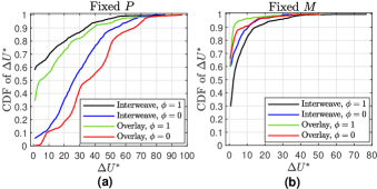
Figure 4: Cumulative distribution function of the percentage increase in objective function, $\Delta U^{*}$, for four different types of opportunistic spectrum access when the sub-optimal algorithm is: (a) optimizing $M$ while holding $P$ fixed. (b) optimizing $P$ while holding $M$ fixed.

V-A Benefit of joint optimization of $M$ and $P$

In our first numerical simulation, we analyze the increase in spectrum utilization that one can obtain using joint optimization of $M$ and $P$ when compared to optimizing $M$ while holding $P$ fixed and vice-versa. Our numerical setup is as follows. There are four candidate licensed operators and no candidate unlicensed operator. There are $10$ parameters which completely defines a market setting: $\mu_{k}^{\theta}$, $\sigma_{k}^{\theta}$, $a_{k}$, $\eta_{k}$, $\rho_{k}$, $\omega_{k}$, $\Lambda_{k}$, $\upsilon$, $\alpha_{L}$, and $\alpha_{U}$. We generate $1000$ such market settings by randomly selecting these $10$ parameters from uniform distributions each of which is associated with a certain range. The range of the parameters $\mu_{k}^{\theta}$, $\sigma_{k}^{\theta}$, $a_{k}$, $\eta_{k}$, $\rho_{k}$, $\omega_{k}$, and $\Lambda_{k}$ for all the operators are $\left[0.75,1.0\right]$, $\left[0.25,0.75\right]$, $\left[0.9,1.1\right]$, $\left[0.25,0.75\right]$, $\left[0.5,0.9\right]$, $\left[0.85,0.95\right]$, and $\left[0.25,1.0\right]$ respectively. The range of $\upsilon$, $\alpha_{L}$, and $\alpha_{U}$ are $\left[0.5,1.0\right]$, $\left[0.75,1.0\right]$, and $\left[0.75,1.0\right]$ respectively. While generating $\alpha_{L}$ and $\alpha_{U}$, we ensure that $\alpha_{L}\leq\alpha_{U}$.

The optimal value of the objective function corresponding to Algorithm 3 is $U^{*}$. We compare Algorithm 3 with a sub-optimal algorithm. Let the optimal value of the objective function corresponding to a sub-optimal algorithm be $\widehat{U}^{*}$. The percentage increase in the objective function is $\Delta U^{*}=\frac{U^{*}-\widehat{U}^{*}}{D}\cdot 100$. The reason for having $D$ in the denominator is as follows. The objective function given by (17) is the mean demand served by all the operators in one time slot which cannot be greater than $D$, the maximum capacity of the entire bandwidth. Hence, $U^{*},\widehat{U}^{*}\leq D$ which implies that $U^{*}-\widehat{U}^{*}\leq D$. We compute $\Delta U^{*}$ for sub-optimal algorithms and plot the cumulative distribution function (CDF) of $\Delta U^{*}$ in Figure 4. Recall that $\phi$ can be $0$ or $1$, and the OSA strategy can be either interweave or overlay. So there are four possible combination of OSA. For a given sub-optimal algorithm, we compute CDFs for all the four combinations.

We consider two sub-optimal algorithms. For the first algorithm, $P$ is fixed and $M$ is optimized. An intuitive choice of $P$ is the number of candidate licensed operators. In that way, every candidate licensed operators wins a licensed channel in every epoch. For the second algorithm, $M$ is fixed and $P$ is optimized. We set $M=\left\lfloor\frac{D}{\vartheta}\right\rfloor$ where $\left\lfloor\cdot\right\rfloor$ is the floor function and $\vartheta=\frac{1}{\left|\mathcal{S}^{C}\right|}\underset{k\in\mathcal{S}^{C}}{\sum}\mu_{k}^{\theta}$ is the sample mean of the mean of an operator’s customer demand. This choice of $M$ is to ensure that the bandwidth $\vartheta$ of a licensed channel is neither too high that most of it is wasted and neither too low that a licensed operator has to reject most of its cushtomer demand.

In Figure 4, a lower value of CDF for a given $\Delta U^{*}$ implies that the difference in spectrum utilization between joint optimization and the sub-optimal algorithm is higher. By comparing Figures 4.a and 4.b we can say that joint optimization leads to more improvement in spectrum utilization when $P$ is fixed rather than when $M$ is fixed. Based on Figure 4.a, we can say that when $P$ is fixed, joint optimization leads to more improvement in spectrum utilization for: (i) overlay strategy than interweave strategy when $\phi$ is fixed. (ii) $\phi=0$ than $\phi=1$. Based on Figure 4.b, we can say that when $M$ is fixed, joint optimization leads to more improvement in spectrum utilization for interweave strategy than overlay strategy when $\phi$ is fixed. We don’t observe any such systematic trend for $\phi$ when $M$ is fixed.

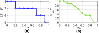
Figure 5: (a) Plots showing the effect of interference parameter $\alpha$ for a market containing only candidate licensed operators on the optimal number of channel, $M^{*}$, and the optimal number of licensed channels, $P^{*}$. (b) Plots showing the effect of interference parameter of licensed channel $\alpha_{L}$ for a market containing both candidate licensed operators and unlicensed operators on the ratio of the bandwidth allocated for unlicensed channels, $\frac{M^{*}-P^{*}}{M^{*}}$.

V-B Effect of interference parameters

Our second numerical simulation is to study the effect of interference parameter on optimal solution. We consider two simulation setups. The first simulation setup is as follows. For this setup, $\alpha_{L}=\alpha_{U}=\alpha$. There are $8$ candidate licensed operators and no candidate unlicensed operators. We consider a homogeneous market setting. The minimum revenue requirement $\lambda_{k}$ is set to zero for all the operators which ensures that all the operators join the market. The remaining parameters of the market are: $\mu_{k}^{\theta}=1$, $\sigma_{k}^{\theta}=0.5$, $a_{k}=1$, $\eta_{k}=0.5$, $\rho_{k}=0.8$, and $\omega_{k}=0.9$ for all $k$’s. Also, $\upsilon=0.8$. We study how $M^{*}$ and $P^{*}$ varies with $\alpha$. The simulation result is shown in Figure 5.a. Since there are no candidate unlicensed operators, it is intuitive that there are no unlicensed channels, i.e. $M^{*}=P^{*}$. Figure 5.a shows that $M^{*}$ decreases with increase in $\alpha$. This can be explained as follows. If $M$ is low, the bandwidth, and hence the capacity of each licensed channel is high. Therefore, a licensed operator can serve more customer demand using the allocated licensed channel thereby increasing spectrum utilization. But if $M$ is too low, only few of the $8$ licensed operators are allocated the licensed channels in an epoch. The remaining operators who uses channels opportunistically as Tier-2 operators. The efficiency of opportunistic access is decided by $\alpha$. If $\alpha$ is low, it is better to have fewer Tier-2 operators in an epoch because opportunistic spectrum access is inefficient. This can be ensured with a higher $M$ so that there are more Tier-1 operators in every epoch.

In our second simulation setup, we include candidate unlicensed operators. The simulation setup is similar to the first setup but differs in the following ways. First, out of the $8$ operators, four are candidate licensed operators and four are candidate unlicensed operators. Second, the interference parameters $\alpha_{L}$ and $\alpha_{U}$ are not same. We set $\alpha_{U}=0.9$ and vary $\alpha_{L}$ from $0$ to $0.9$. We study how the ratio of the bandwidth allocated for unlicensed channels characterized by the ratio $\frac{M^{*}-P^{*}}{M^{*}}$ changes with $\alpha_{L}$. This is shown in Figure 5.b. Unlike the previous simulation setup, the current simulation setup has candidate unlicensed operators. Therefore, we expect that there will be unlicensed channels dedicated for the candidate unlicensed operators. But the question is: what portion of the bandwidth should be allocated for unlicensed channels? If $\alpha_{L}$ is high, most of the bandwidth can be reserved for licensed channels because even if the Tier-1 operators are not using the licesnsed channels, the Tier-2 operators can use the remaining capacity of the licensed channels efficiently. But as $\alpha_{L}$ decreases, the opportunistic access of licensed channels becomes inefficient. Therefore, it is better to reserve higher portion of the bandwidth for unlicensed channels.

V-C Market competition vs Spectrum Utilization

For most markets, an increase in competition improves the social welfare. In our setup, we use the number of interested operators, $\left|\mathcal{S}_{L}\right|+\left|\mathcal{S}_{U}\right|$, as the measure of market competition and spectrum utilization as the measure of social welfare. In this numerical simulation, we show that there exists market setups where an increase in $\left|\mathcal{S}_{L}\right|+\left|\mathcal{S}_{U}\right|$ decreases spectrum utilization. The simulation setup and the definition of $\Delta U^{*}$ is similar to Section V-A but differs in the following ways. First, in this setup we have three candidate licensed operators and three candidate unlicensed operators. Second, the sub-optimal algorithm in this setup finds $M$ and $P$ that maximize $\left|\mathcal{S}_{L}\right|+\left|\mathcal{S}_{U}\right|$ instead of the objective function defined in equation (17). If there are multiple values of $M$ and $P$ that maximize $\left|\mathcal{S}_{L}\right|+\left|\mathcal{S}_{U}\right|$, we choose the ones that maximize the objective function defined in equation (17).

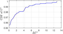
Figure 6: Cumulative distribution function of the percentage increase in objective function, $\Delta U^{*}$, when the sub-optimal algorithm is to choose the value of $M$ and $P$ that maximize the number of interested operators.

The simulation result is shown in Figure 6 where we plot the CDF of $\Delta U^{*}$ for $1000$ market setups. To establish our claim that maximizing $\left|\mathcal{S}_{L}\right|+\left|\mathcal{S}_{U}\right|$ doesn’t necessarily maximize spectrum utilization, we want to find market setups where $\Delta U^{*}$ is strictly greater than $0$. We can see that for $\left(1-0.955\right)\cdot 100\%=4.5\%$ of the market setups, $\Delta U^{*}>0$. This establishes our claim that there are market setups, however few, where maximizing $\left|\mathcal{S}_{L}\right|+\left|\mathcal{S}_{U}\right|$ doesn’t necessarily maximize spectrum utilization. However, for these $4.5\%$ of the market setups, $\Delta U^{*}$ is upper bounded by $13\%$ implying only a marginal improvement in spectrum utilization.

VI Conclusion

In this paper, we designed an optimization algorithm to partition a bandwidth into channels and further decide the number of licensed channels in order to maximize spectrum utilization. The access to this bandwidth is governed by a tiered spectrum access model inspired by the CBRS band. We first propose a system model which accurately captures various aspects of the tiered spectrum access model. Based on this model, we formulate our optimization problem as a two-staged Stackelberg game and then designed algorithms to solve the Stackelberg game. Finally, we get numerical results to benchmark our algorithm and to also study certain optimal trends of spectrum partitioning and licensing as a function of interference parameters.

There can be various directions for future research related to generalization of the Stackelberg Game model. First, is to capture collusion between operators in Stage-2 of the Stackelberg Game. Second, in our current model, every operator is assumed to be equally pessimistic. It would be interesting to associate each operator with a degree of pessimism.

Appendix A Proof of Proposition 2

Throughout this derivation, $t$ represents the $t^{th}$ time slot of $\gamma^{th}$ epoch, i.e. $t\in\left[\left(\gamma-1\right)T+1,\gamma T\right]$. We start by deriving the stochastic model between $\theta_{k}\left(t\right)$ and $X_{k,lc}\left(\gamma\right)$, the net demand served by the $k^{th}$ operator in $\gamma^{th}$ epoch using licensed spectrum access. For Gaussian random variables $\theta_{k}\left(t\right)$ and $X_{k,lc}\left(\gamma\right)$, their joint Gaussian distribution is characterised by their mean and their covariance matrix. The mean and the variance of $\theta_{k}\left(t\right)$ are $\mu_{k}^{\theta}$ and $\left(\sigma_{k}^{\theta}\right)^{2}$ respectively. The mean and the variance of $X_{k,lc}\left(\gamma\right)$ are $\mu_{k,lc}^{X}$ and $\left(\sigma_{k,lc}^{X}\right)^{2}$ respectively. So, to find the joint Gaussian distribution of $\theta_{k}\left(t\right)$ and $X_{k,lc}\left(\gamma\right)$, all we have to derive is the covariance of $\theta_{k}\left(t\right)$ and $X_{k,lc}\left(\gamma\right)$. To do so, we are going to first recall few notations from Section II-B. We have, $x_{k}\left(t\right)=\max\left(0,\theta_{k}\left(t\right)\right)$, $\widetilde{x}_{k,lc}\left(t\right)=\min\left(x_{k}\left(t\right),\frac{D}{M}\right)$ and $X_{k,lc}\left(\gamma\right)=\stackrel{{\scriptstyle[}}{{t}}=\left(\gamma-1\right)T+1]{\gamma T}{\sum}\widetilde{x}_{k,lc}\left(t\right)$. Define,

$$\overline{X}_{k,lc}\left(\gamma,t\right)=\stackrel{{\scriptstyle[}}{{v}}=\left(\gamma-1\right)T+1]{t-1}{\sum}\widetilde{x}_{k,lc}\left(v\right)+\stackrel{{\scriptstyle[}}{{v}}=t+1]{\gamma T}{\sum}\widetilde{x}_{k,lc}\left(v\right)$$ (38)

where, $\widetilde{x}_{k,lc}\left(v\right)=\min\left(\max\left(0,\theta_{k}\left(v\right)\right),\frac{D}{M}\right)$. The mean of $\overline{X}_{k,lc}\left(\gamma,t\right)$ is $E\left[\overline{X}_{k,lc}\left(\gamma,t\right)\right]=\widetilde{\mu}_{k,lc}^{x}\left(T-1\right)$. The covariance of $\theta_{k}\left(t\right)$ and $X_{k,lc}\left(\gamma\right)$ is

$$\varphi_{k} = E\left[\left(\theta_{k}\left(t\right)-\mu_{k}^{\theta}\right)\left(X_{k,lc}\left(\gamma\right)-\mu_{k,lc}^{X}\right)\right]$$ (39)

$$= E\left[\left(\theta_{k}\left(t\right)-\mu_{k}^{\theta}\right)\left(\overline{X}_{k,lc}\left(\gamma,t\right)-\widetilde{\mu}_{k,lc}^{x}\left(T-1\right)\right)\right.$$

$$\left.\quad+\left(\theta_{k}\left(t\right)-\mu_{k}^{\theta}\right)\left(\widetilde{x}_{k,lc}\left(t\right)-\widetilde{\mu}_{k,lc}^{x}\right)\right]$$

$$= E\left[\left(\theta_{k}\left(t\right)-\mu_{k}^{\theta}\right)\left(\overline{X}_{k,lc}\left(\gamma,t\right)-\widetilde{\mu}_{k,lc}^{x}\left(T-1\right)\right)\right]$$

$$+E\left[\left(\theta_{k}\left(t\right)-\mu_{k}^{\theta}\right)\left(\widetilde{x}_{k,lc}\left(t\right)-\widetilde{\mu}_{k,lc}^{x}\right)\right]$$

In (39), $\theta_{k}\left(t\right)$ and $\overline{X}_{k,lc}\left(\gamma,t\right)$ are independent random variables. This is because $\theta_{k}\left(t\right)$ are iid random variables and according to (38), $\overline{X}_{k,lc}\left(\gamma,t\right)$ is not directly dependent on $\theta_{k}\left(t\right)$. Therefore, the first term of (39) is zero. We have,

$$\varphi_{k} = E\left[\left(\theta_{k}\left(t\right)-\mu_{k}^{\theta}\right)\left(\widetilde{x}_{k,lc}\left(t\right)-\widetilde{\mu}_{k,lc}^{x}\right)\right]$$

$$= E\left[\theta_{k}\left(t\right)\widetilde{x}_{k,lc}\left(t\right)\right]-\mu_{k}^{\theta}\widetilde{\mu}_{k,lc}^{x}$$

$$= E\left[\theta_{k}\left(t\right)\min\left(\max\left(0,\theta_{k}\left(t\right)\right),\frac{D}{M}\right)\right]-\mu_{k}^{\theta}\widetilde{\mu}_{k,lc}^{x}$$

$$\qquad=\stackrel{{\scriptstyle[}}{{0}}]{\frac{D}{M}}{\int}\vartheta^{2}f_{k}^{\theta}\left(\vartheta\right)\,d\vartheta+\frac{D}{M}\stackrel{{\scriptstyle[}}{{\frac{}}{missing}}{D}{M}]{\infty}{\int}\vartheta f_{k}^{\theta}\left(\vartheta\right)\,d\vartheta-\mu_{k}^{\theta}\widetilde{\mu}_{k,lc}^{x}$$ (40)

where, $f_{k}^{\theta}\left(\vartheta\right)$ is the probability density function of $\theta_{k}\left(t\right)$. To this end, we have derived the joint Gaussian distribution of $\theta_{k}\left(t\right)$ and $X_{k,lc}\left(\gamma\right)$. We have,

$$\begin{bmatrix}\theta_{k}\left(t\right)\\ X_{k,lc}\left(\gamma\right)\end{bmatrix}\sim\mathcal{N}\left(\begin{bmatrix}\mu_{k}^{\theta}\\ \mu_{k,lc}^{X}\end{bmatrix},\begin{bmatrix}\left(\sigma_{k}^{\theta}\right)^{2}&\varphi_{k}\\ \varphi_{k}&\left(\sigma_{k,lc}^{X}\right)^{2}\end{bmatrix}\right)$$ (41)

The joint Gaussian distribution of $\theta_{k}\left(t\right)$ and $X_{k,lc}\left(\gamma\right)$ is given by (41), that of $R_{k,lc}\left(\gamma\right)$ and $X_{k,lc}\left(\gamma\right)$ is given by (7) and that of $R_{k,lc}\left(\gamma\right)$ and $V_{k}\left(\gamma\right)$ is given by (10). We want to derive the joint Gaussian distribution of $\theta_{k}\left(t\right)$, $R_{k,lc}\left(\gamma\right)$ and $V_{k}\left(\gamma\right)$. Just like $\theta_{k}\left(t\right)$ and $X_{k,lc}\left(\gamma\right)$, all we need to know to derive the joint Gaussian distribution of $\theta_{k}\left(t\right)$, $R_{k,lc}\left(\gamma\right)$ and $V_{k}\left(\gamma\right)$ are their mean and covariance matrix. We have already discussed the mean and variance of $\theta_{k}\left(t\right)$ in the beginning of this section. The mean and variance of both $R_{k,lc}\left(\gamma\right)$ and $V_{k}\left(\gamma\right)$ are $\mu_{k,lc}^{R}$ and $\left(\sigma_{k,lc}^{R}\right)^{2}$ respectively (refer to (10)). According to (10), the covariance of $R_{k,lc}\left(\gamma\right)$ and $V_{k}\left(\gamma\right)$ is $\omega{}_{k}\left(\sigma_{k,lc}^{R}\right)^{2}$. All we have to derive is the covariance of two set of random variables. First, $\theta_{k}\left(t\right)$ and $R_{k,lc}\left(\gamma\right)$ and second, $\theta_{k}\left(t\right)$ and $V_{k}\left(\gamma\right)$. The following proposition is important for this derivation.

Proposition 3.

Consider jointly Gaussian variables $A$ and $B$,

$$\begin{bmatrix}A\\ B\end{bmatrix}\sim\mathcal{N}\left(\begin{bmatrix}\mu_{A}\\ \mu_{B}\end{bmatrix},\begin{bmatrix}\sigma_{A}^{2}&\sigma_{AB}\\ \sigma_{AB}&\sigma_{B}^{2}\end{bmatrix}\right)$$ (42)

where $\mu_{A}$ and $\sigma_{A}$ are the mean and standard deviation of $A$ respectively, $\mu_{B}$ and $\sigma_{B}$ are the mean and standard deviation of $B$ respectively and $\rho_{AB}$ is the correlation coefficient of $A$ and $B$. Let $\mathcal{L}\left(A\,|\,B=b\right)$ denote the conditional distribution of $A$ given $B=b$. Then, $\mathcal{L}\left(A\,|\,B=b\right)$ is a Gaussian distribution with mean $\mu_{A}+\frac{\sigma_{AB}}{\sigma_{B}^{2}}\left(b-\mu_{B}\right)$ and standard deviation $\sqrt{\sigma_{A}^{2}-\frac{\sigma_{AB}^{2}}{\sigma_{B}^{2}}}$. Mathematically,

$${\textstyle\mathcal{L}\left(A\,|\,B=b\right)=}\mathcal{N}\left(\mu_{A}+\frac{\sigma_{AB}}{\sigma_{B}^{2}}\left(b-\mu_{B}\right),\left(\sigma_{A}^{2}-\frac{\sigma_{AB}^{2}}{\sigma_{B}^{2}}\right)\right)$$ (43)

Proof:

The proof of a generalized version of this proposition can be found in [29, Chapter 3]. ∎

The covariance of $\theta_{k}\left(t\right)$ and $R_{k,lc}\left(\gamma\right)$ is

$$\overline{\varphi}_{k}=E\left[\left(\theta_{k}\left(t\right)-\mu_{k}^{\theta}\right)\left(R_{k,lc}\left(\gamma\right)-\mu_{k,lc}^{R}\right)\right]$$ (44)

Let $f_{k}^{X}\left(\phi\right)$ be the probability density function of $X_{k,lc}\left(\gamma\right)$. Define,

$${\textstyle h\left(\phi\right)=E\left[\left(\theta_{k}\left(t\right)-\mu_{k}^{\theta}\right)\left(R_{k,lc}\left(\gamma\right)-\mu_{k,lc}^{R}\right)\mid X_{k,lc}\left(\gamma\right)=\phi\right]}$$ (45)

where $h\left(\phi\right)$ is the covariance of $\theta_{k}\left(t\right)$ and $R_{k,lc}\left(\gamma\right)$ conditioned on $X_{k,lc}\left(\gamma\right)=\phi$. Using the law of total expectation, (44) can be equivalently written as

$$\overline{\varphi}_{k} = \stackrel{{\scriptstyle[}}{{-}}\infty]{\infty}{\int}h\left(\phi\right)f_{k}^{X}\left(\phi\right)\,d\phi$$ (46)

Based on (41) and (7), if $X_{k,lc}\left(\gamma\right)$ is given, $R_{k,lc}\left(\gamma\right)$ and $\theta_{k}\left(t\right)$ are independent of each other. Therefore, (45) can be equivalently written as

$$h\left(\phi\right) = E\left[\left(\theta_{k}\left(t\right)-\mu_{k}^{\theta}\right)\mid X_{k,lc}\left(\gamma\right)=\phi\right]$$ (47)

$$\cdot E\left[\left(R_{k,lc}\left(\gamma\right)-\mu_{k,lc}^{R}\right)\mid X_{k,lc}\left(\gamma\right)=\phi\right]$$

$$= \left(E\left[\theta_{k}\left(t\right)\mid X_{k,lc}\left(\gamma\right)=\phi\right]-\mu_{k}^{\theta}\right)$$

$$\cdot\left(E\left[R_{k,lc}\left(\gamma\right)\mid X_{k,lc}\left(\gamma\right)=\phi\right]-\mu_{k,lc}^{R}\right)$$

Using (41) and Proposition 3,

$$E\left[\theta_{k}\left(t\right)\mid X_{k,lc}\left(\gamma\right)=\phi\right]=\mu_{k}^{\theta}+\frac{\varphi_{k}}{\left(\sigma_{k,lc}^{X}\right)^{2}}\left(\phi-\mu_{k,lc}^{X}\right)$$ (48)

Using (7) and Proposition 3,

$$E\left[R_{k,lc}\left(\gamma\right)\mid X_{k,lc}\left(\gamma\right)=\phi\right]=\mu_{k,lc}^{R}+\frac{\rho_{k}\sigma_{k,lc}^{X}\sigma_{k,lc}^{R}}{\left(\sigma_{k,lc}^{X}\right)^{2}}\left(\phi-\mu_{k,lc}^{X}\right)$$ (49)

Substituting (47), (48) and (49) in (46) we get,

$$\overline{\varphi}_{k} = \frac{\rho_{k}\sigma_{k,lc}^{R}\varphi_{k}}{\left(\sigma_{k,lc}^{X}\right)^{3}}\stackrel{{\scriptstyle[}}{{-}}\infty]{\infty}{\int}\left(\phi-\mu_{k,lc}^{X}\right)^{2}f_{k}^{X}\left(\phi\right)\,d\phi$$ (50)

The integral in (50) is the variance of $X_{k,lc}\left(\gamma\right)$ which is equal to $\left(\sigma_{k,lc}^{X}\right)^{2}$. Therefore, (50) is equal to

$$\overline{\varphi}_{k}=\frac{\rho_{k}\sigma_{k,lc}^{R}\varphi_{k}}{\left(\sigma_{k,lc}^{X}\right)^{3}}\left(\sigma_{k,lc}^{X}\right)^{2}=\rho_{k}\frac{\sigma_{k,lc}^{R}}{\sigma_{k,lc}^{X}}\varphi_{k}$$ (51)

Now, we have to derive the covariance of $\theta_{k}\left(t\right)$ and $V_{k}\left(\gamma\right)$. This derivation is same as the derivation for the covariance of $\theta_{k}\left(t\right)$ and $R_{k,lc}\left(\gamma\right)$ and has been skipped for brevity. We simply state that the covariance of $\theta_{k}\left(t\right)$ and $V_{k}\left(\gamma\right)$ is $\omega_{k}\rho_{k}\frac{\sigma_{k,lc}^{R}}{\sigma_{k,lc}^{X}}\varphi_{k}$. Finally, based on our derivation, the mean, $\psi_{k}$, and the covariance matrix, $\Sigma_{k}$, of $\theta_{k}\left(t\right)$, $R_{k,lc}\left(\gamma\right)$ and $V_{k}\left(\gamma\right)$ are given by (32) and (33) respectively. Hence, the joint probability distribution of $\theta_{k}\left(t\right)$, $R_{k,lc}\left(\gamma\right)$ and $V_{k}\left(\gamma\right)$ is given by (31). This completes the proof.

References

- [1] Federal Communications Commission, “Amendment of the commission’s rules with regard to commercial operations in the 3550-3650 mhz band,” 2015. [Online]. Available: https://docs.fcc.gov/public/attachments/FCC-15-47A1.pdf
- [2] ——, “Amendment of the commission’s rules with regard to commercial operations in the 3550-3650 mhz band,” 2016. [Online]. Available: https://docs.fcc.gov/public/attachments/FCC-16-55A1.pdf
- [3] ——, “Promoting investment in the 3550-3700 mhz band,” 2017. [Online]. Available: https://docs.fcc.gov/public/attachments/FCC-17-134A1.pdf
- [4] N. Jindal, J. G. Andrews, and S. Weber, “Bandwidth partitioning in decentralized wireless networks,” IEEE Transactions on Wireless Communications, vol. 7, no. 12, pp. 5408–5419, 2008.
- [5] X. Feng, P. Lin, and Q. Zhang, “Flexauc: Serving dynamic demands in a spectrum trading market with flexible auction,” IEEE Transactions on Wireless Communications, vol. 14, no. 2, pp. 821–830, 2014.
- [6] Q. Liang, H.-W. Lee, and E. Modiano, “Robust design of spectrum-sharing networks,” IEEE Transactions on Mobile Computing, vol. 18, no. 8, pp. 1924–1937, 2019.
- [7] X. Lin and J. G. Andrews, “Optimal spectrum partition and mode selection in device-to-device overlaid cellular networks,” in 2013 IEEE global communications conference (GLOBECOM). IEEE, 2013, pp. 1837–1842.
- [8] C. Bazelon, “Licensed or unlicensed: The economic considerations in incremental spectrum allocations,” IEEE Communications Magazine, vol. 47, no. 3, pp. 110–116, 2009.
- [9] T. Nguyen, H. Zhou, R. A. Berry, M. L. Honig, and R. Vohra, “The impact of additional unlicensed spectrum on wireless services competition,” in 2011 IEEE International Symposium on Dynamic Spectrum Access Networks (DySPAN). Citeseer, 2011, pp. 146–155.
- [10] A. Ghosh and R. Berry, “Competition with three-tier spectrum access and spectrum monitoring,” in Proceedings of the Twentieth ACM International Symposium on Mobile Ad Hoc Networking and Computing, 2019, pp. 241–250.
- [11] ——, “Entry and investment in cbrs shared spectrum,” in 2020 18th International Symposium on Modeling and Optimization in Mobile, Ad Hoc, and Wireless Networks (WiOPT). IEEE, 2020, pp. 1–8.
- [12] C. Chen, R. A. Berry, M. L. Honig, and V. G. Subramanian, “Competitive resource allocation in hetnets: The impact of small-cell spectrum constraints and investment costs,” IEEE Transactions on Cognitive Communications and Networking, vol. 3, no. 3, pp. 478–490, 2017.
- [13] K. Zhu, E. Hossain, and D. Niyato, “Pricing, spectrum sharing, and service selection in two-tier small cell networks: A hierarchical dynamic game approach,” IEEE Transactions on Mobile Computing, vol. 13, no. 8, pp. 1843–1856, 2013.
- [14] X. Feng, Q. Zhang, and B. Li, “Head: A hybrid spectrum trading framework for qos-aware secondary users,” in Dynamic Spectrum Access Networks (DYSPAN), 2014 IEEE International Symposium on. IEEE, 2014, pp. 489–497.
- [15] Y. Chen, L. Duan, J. Huang, and Q. Zhang, “Balancing income and user utility in spectrum allocation,” IEEE Transactions on Mobile Computing, vol. 14, no. 12, pp. 2460–2473, 2015.
- [16] M. R. Hassan, G. C. Karmakar, J. Kamruzzaman, and B. Srinivasan, “Exclusive use spectrum access trading models in cognitive radio networks: A survey,” IEEE Communications Surveys & Tutorials, vol. 19, no. 4, pp. 2192–2231, 2017.
- [17] Y. Chen, P. Lin, and Q. Zhang, “Lotus: Location-aware online truthful double auction for dynamic spectrum access,” in 2014 IEEE International Symposium on Dynamic Spectrum Access Networks (DYSPAN). IEEE, 2014, pp. 510–518.
- [18] S. Ross, A First Course in Probability, 8th ed. Pearson, 2009.
- [19] A. Asheralieva, “Prediction based bandwidth allocation for cognitive lte network,” in 2013 IEEE Wireless Communications and Networking Conference (WCNC). IEEE, 2013, pp. 801–806.
- [20] A. Sahoo, “Fair resource allocation in the citizens broadband radio service band,” in 2017 IEEE International Symposium on Dynamic Spectrum Access Networks (DySPAN). IEEE, 2017, pp. 1–2.
- [21] D. P. Bertsekas, R. G. Gallager, and P. Humblet, Data networks. Prentice-Hall International New Jersey, 1992, vol. 2.
- [22] B. Radunovic and J.-Y. Le Boudec, “A unified framework for max-min and min-max fairness with applications,” IEEE/ACM Transactions on networking, vol. 15, no. 5, pp. 1073–1083, 2007.
- [23] Y. Tohidi, M. R. Hesamzadeh, and F. Regairaz, “Sequential coordination of transmission expansion planning with strategic generation investments,” IEEE Transactions on Power Systems, vol. 32, no. 4, pp. 2521–2534, 2016.
- [24] I. Gilboa, Theory of decision under uncertainty. Cambridge university press, 2009, vol. 45.
- [25] E. Hasan and F. D. Galiana, “Electricity markets cleared by merit order - part ii: strategic offers and market power,” IEEE Transactions on Power Systems, vol. 23, no. 2, pp. 372–379, 2008.
- [26] K. Leyton-Brown and Y. Shoham, “Essentials of game theory: A concise multidisciplinary introduction,” Synthesis lectures on artificial intelligence and machine learning, vol. 2, no. 1, pp. 1–88, 2008.
- [27] A. Mas-Colell, M. D. Whinston, J. R. Green et al., Microeconomic theory. Oxford university press New York, 1995, vol. 1.
- [28] B. Welford, “Note on a method for calculating corrected sums of squares and products,” Technometrics, vol. 4, no. 3, pp. 419–420, 1962.
- [29] M. L. Eaton, “Multivariate statistics: a vector space approach.” JOHN WILEY & SONS, INC., 605 THIRD AVE., NEW YORK, NY 10158, USA, 1983, 512, 1983.