Determination of responses of liquid xenon to low energy electron and nuclear recoils using the PandaX-II detector

Abstract

We report a systematic determination of the responses of PandaX-II, a dual phase xenon time projection chamber detector, to low energy recoils. The electron recoil (ER) and nuclear recoil (NR) responses are calibrated, respectively, with injected tritiated methane or ²²⁰Rn source, and with ²⁴¹Am-Be neutron source, within an energy range from $1-25$ keV (ER) and $4-80$ keV (NR), under the two drift fields of 400 and 317 V/cm. An empirical model is used to fit the light yield and charge yield for both types of recoils. The best fit models can well describe the calibration data. The systematic uncertainties of the fitted models are obtained via statistical comparison against the data.

Keywords: dark matter, liquid xenon time projection chamber, calibration, electron recoil, nucleon recoil, NEST2.0

1 Introduction

The nature of dark matter (DM) remains to be one of the most intriguing physics questions today. The direct search for an important class of dark matter candidate, the weakly interacting massive particles (WIMPs), has been accelerated by the development in dual phase xenon time projection chambers (TPCs), such as PandaX-II [1], XENON-1T [2], and LUX [3]. In these detectors, a WIMP may interact with xenon nuclei via elastic scattering, depositing a nuclear recoil (NR) energy from few keV_nr to a few tens of keV_nr. $\gamma$s or $\beta$s from internal impurities and detector materials produce electron recoil (ER) background events, which have a small probability to be identified as the NR signals in these detectors.

In a dual phase xenon TPC bounded by a cathode at the bottom in the liquid and an anode at the top in the gas, each energy deposition will be converted into two channels, the scintillation photons and ionized electrons. The former is the so-called $S1$ signal. Electrons are subsequently drifted towards the liquid surface, and extracted into the gas region with delayed electroluminescence photons ($S2$) produced. Both $S1$s and $S2$s are collected by two arrays of photomultiplier tubes (PMTs) located at the top and bottom of the TPC. For a given event, the combination of $S1$ and $S2$ allows the reconstruction of the recoil energy and vertex, and the proportion of $S1$ and $S2$ serves as a key discriminant for ER and NR. It is essential to determine the detector response via in situ calibration.

For the ER response, several injected sources were used in PandaX-II, including tritiated methane (CH₃T), ²²⁰Rn, and ^83mKr. For NR calibration, an external ²⁴¹Am-Be (AmBe) neutron source was used. In this paper, the detector responses are determined by fitting these data under the NEST2.0 [4] prescription.

This rest of this paper is organized as follows. In Sec. 2, the detector conditions and calibration setups are introduced. In Sec. 3, data processing and event selection cuts are presented. The response model simulation will be introduced in Sec. 4, followed by detailed discussions on the fits of the light yield and charge yield, before the conclusion in Sec. 5.

2 Calibration setup

The PandaX-II experiment, located at the China Jinping underground laboratory (CJPL) [5], was under operation from March 2016 to July 2019, with a total exposure of 132 ton$\cdot$day for dark matter search. The operation was divided into three runs, Runs 9, 10, and 11 [6], during which calibration runs were interleaved. The detector contained 580-kg liquid xenon in its sensitive volume. The liquid xenon was continuously purified through two circulation loops, each connected to a getter purifier. The internal ER sources were injected through one of the loop. Two PTFE tubes, at 1/4 and 3/4 height of the TPC surrounding the inner cryostat, were used as the guide tube for the external AmBe source. The TPC drift field in Run 9 was 400 V/cm and 317 V/cm in Runs 10/11, corresponding to a maximum drift time of 350 $\mu$s and 360 $\mu$s, respectively. The running conditions, key detector parameters, and event selection ranges for the calibration data sets are summarized in Table. 1.

Data set	Run9 AmBe	Run9 Tritium	Runs 10/11 AmBe	Runs 10/11 220Rn
PDE	0.115$\pm$0.002		0.120$\pm$0.005
EEE	0.463$\pm$0.014		0.475$\pm$0.020
SEG	24.4$\pm$0.4		23.5 $\pm$0.8
$E_{\rm{drift}}$ (V/cm)	400		317
$E_{\rm{extract}}$ (kV/cm)	4.56
Duration (day)	6.7	27.9	48.5	11.9
Number of events	2902	9387	11196	8841
Drift time cut($\mu s$)	18-200	18-310	50-200	50-350
range cut	S1:3-150 PE S2:100-20000 PE	$E_{\rm{rec}}$¡25 keV	S1:3-150 PE S2:100-20000 PE	$E_{\rm{rec}}$¡25 keV

Table 1: Summary of ER and NR calibration data sets and corresponding detector configurations. PDE, EEE, and SEG, respectively, are the photon detection efficiency, electron extraction efficiency, and single electron gain. $E_{\rm drift}$ and $E_{\rm extract}$ are the drift field and extraction field. The number of events correspond to the calibration data after all cuts, which are described in Sec. 3.

2.1 Tritiated methane

Tritiated methane calibration was first developed in the LUX experiment [7], which provided excellent internal low energy $\beta$ events. The tritiated methane source used in PandaX-II was procured from American Radio labeled Chemicals, Inc., with a specific activity of 0.1 Curie per mole of methane. The injection diagram is shown in Fig. 1. The tritiated methane bottle was immersed in a liquid-nitrogen cold trap, so that controllable amount of the CH₃T gas could diffuse through a needle valve to the 100 mL mixing volume. The gas in the mixing volume was flushed with xenon gas into the detector.

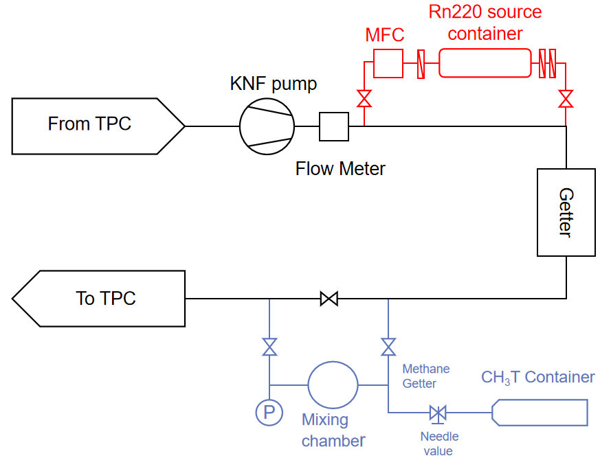
Figure 1: Tritiated methane (blue) and ²²⁰Rn (red) injection system.

The injection of tritium was performed in 2016 right after Run 9, during which about 5.4$\times 10^{-10}$ mol of methane was loaded into the detector. The tritium events were distributed uniformly in the detector. Liquid xenon was constantly circulated at a speed of about 40 SLPM (standard liter of gas per minute) through the purifier. The entire calibration run lasted for 44 days, and the later data set with an average electron lifetime of 706 $\mu$s is used as the ER calibration data.

It was realized that the hot getters were inefficient to remove tritium, whose activity plateaued at 10.2 $\mu$Bq/kg. A distillation campaign was carried out after the calibration, which reduced the tritium activity to 0.049$\pm$0.005 $\mu$Bq/kg in Runs 10/11 [6].

2.2 ²²⁰Rn

²²⁰Rn, a decay progeny of ²³²Th, is a naturally occurring radioactive noble gas isotope. With a half-life of 55 s, it poses much less risk to contaminate the liquid xenon TPC, as first demonstrated in XENON100 [8]. The details of ²²⁰Rn calibration setup and operation in PandaX-II can be found in Ref. [9]. The injection system consisting of a mass flow controller and a ²³²Th source chamber with filters upstream and downstream, is shown in Fig. 1. After ²²⁰Rn was injected into the detector, the $\beta$-decay of the daughter nucleus ²¹²Pb gives uniformly distributed ER events with an energy extending to zero. 11.9 days of ²²⁰Rn data in 2018 are used as the low energy ER calibration for Runs 10/11.

2.3 AmBe

Neutron calibration data with an AmBe ($\alpha$, n) source [10] were taken during Run 9 and Runs 10/11. The source was placed inside the external calibration tubes. Calibration runs were taken at eight symmetric locations in each loop to evenly sample the detector. For different source locations, no significant difference is identified in the detector response, so the data are grouped together in the analysis.

3 Data selection

The processing of the calibration data follows the procedure in Ref. [6]. Compared to previous analyses [1, 11], seven unstable PMTs are inhibited from all data sets for consistency. Improvements are made on the PMT gain calibration, quality cuts, position reconstruction, and corresponding non-uniformity correction.

The raw $S1$ and $S2$ of each event have to be first corrected for position non-uniformity, based on the three-dimensional variation of the raw $S1$ and $S2$ for the uniformly distributed mono-energetic events, e.g. 164 keV (^131mXe) due to activation from the neutron source. The correction to $S1$ is a smooth three-dimensional hyper-surface. The correction to $S2$ is separated into an exponential attenuation vs. drift time (electron lifetime $\tau$), and a smooth two-dimensional surface in the horizontal plane.

The electron equivalent energy of each event is reconstructed as

$$E_{\rm{rec}}=W\times\left(\frac{S1}{\rm{PDE}}+\frac{S2}{\rm{EEE}\times\rm{SEG}}\right)$$ (1)

where $W=13.7$ eV [12] is the average energy to produce either a scintillation photon or free electron in liquid xenon, and PDE, EEE, and SEG, respectively, are the photon detection efficiency (ratio of detected photoelectrons to the total photons), electron extraction efficiency, and single electron gain, obtained from the data (see Ref. [6] and Table. 1).

Events with a single pair of $S1$ and $S2$ are chosen. Fiducial volume (FV) definition is consistent with Ref. [6], except that a lower cut in drift time (200 ${\mu}$s) is applied to the AmBe data to avoid events that multi-scatter and deposit part of the energy in the below-cathode region, leading to suppressed $S2$ [11]. The lower selection cuts $S1>3$ PE and $S2_{\rm raw}>100$ PE are applied to all data sets. For the AmBe data, the upper selection cut is set at $S1<150$ PE ($\sim$80 keV_nr). For ER data, events with $E_{\rm rec}<25$ keV are selected. The vertex distributions of selected events are shown in Fig. 2, with FV cuts indicated. The distributions of $S2$ vs. $S1$ for ER and NR events are shown in Fig. 3, which will be used to determine the detector response model.

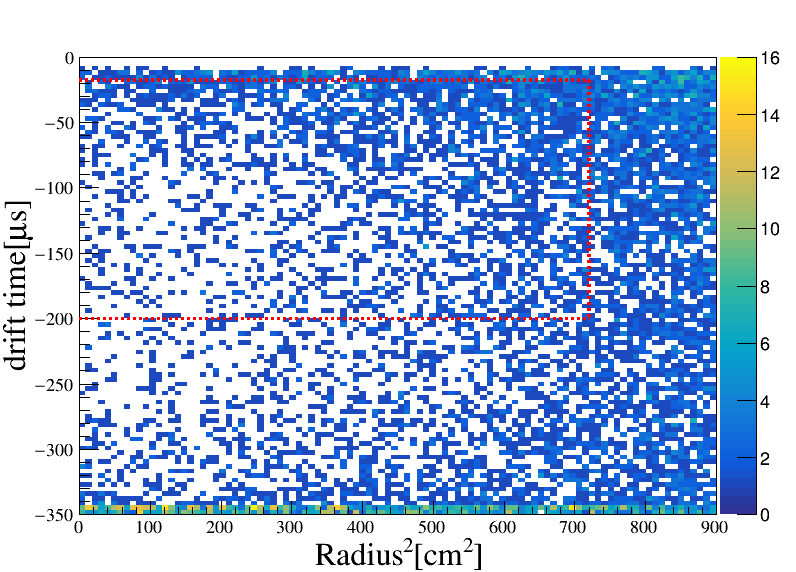
(a) Run 9 AmBe

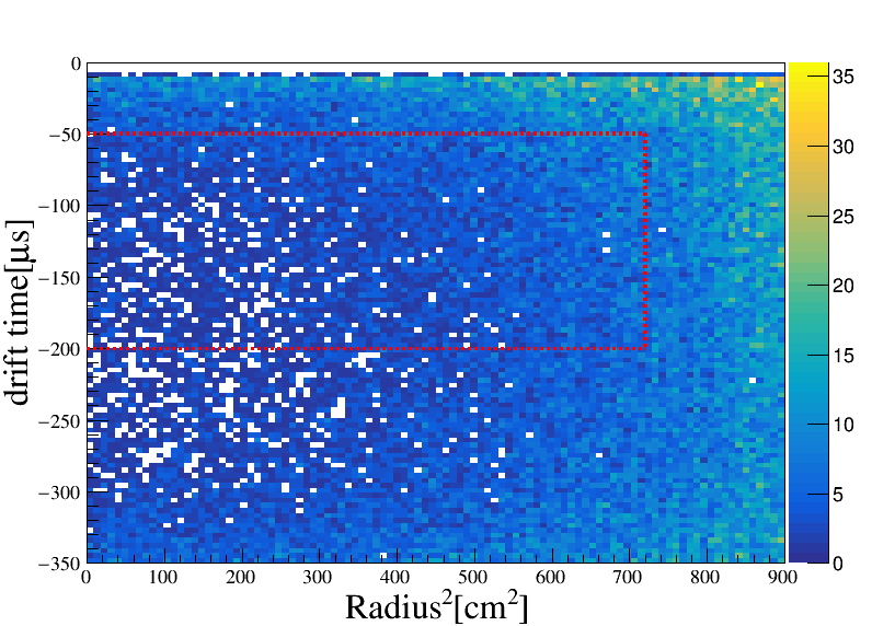
(b) Runs 10/11 AmBe

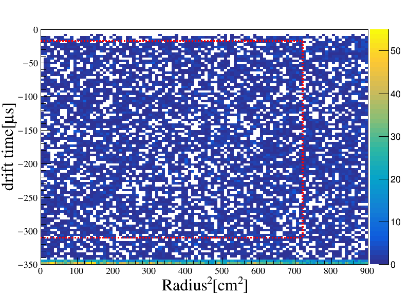
(c) Run 9 tritium

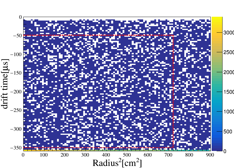
(d) Runs 10/11 Radon

Figure 2: Event vertex distribution in drift time vs. radius-squared for each calibration data set. The FV region is indicated by dashed red line in each figure.

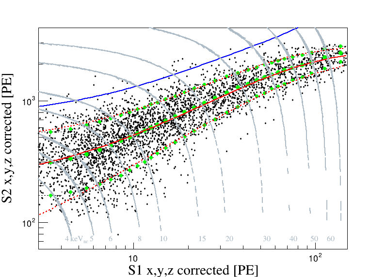
(a) AmBe in Run9

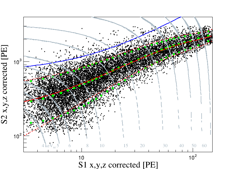
(b) AmBe in Runs 10/11

(c) Tritium in Run 9

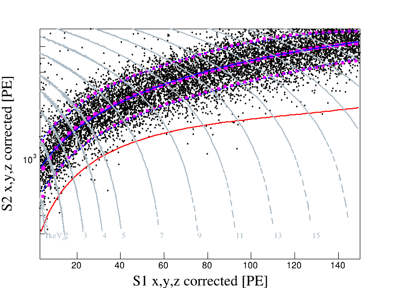
(d) Radon in Runs 10/11

Figure 3: $S2$ vs. $S1$ of the selected calibration events. The red (blue) solid lines are the medians of NR (ER), and the red (blue) dashed lines refer to the 90% quantiles. For comparison, the 90% quantiles from the best fit response models (Sec. 4) are overlaid as the green (purple) dotted lines for NR (ER). The gray dashed curves are the equal-$E_{\rm nr}$ and equal-$E_{\rm rec}$ lines for the NR and ER events, respectively.

4 Determination of PandaX-II response models

Our ER and NR response models follow the prescription of NEST2.0 [4], but use our own customization. The light yield ($L_{y}$) and charge yield ($Q_{y}$), defined as the number of initial quanta (photons or ionized electrons) per unit recoil energy, can be parameterized and fitted to the calibration data. We shall discuss the simulation models in Sec. 4.1 and Sec. 4.2, which will be then fitted to data in Sec. 4.3

4.1 Quanta generation

For a distribution of true recoil energy from the calibration source, each recoil energy $E_{0}$ is converted into two types of quanta, scintillation photons $n_{\rm ph}^{0}$ or ionized electrons $n_{\rm e}^{0}$. For the NRs, the visible energy is quenched into $E_{0}\times L$ due to unmeasurable dissipation of heat in the recoil, where $L$ is the so-called Linhard factor with a value ranging from 0.1 to 0.25 for $E_{0}$ less than 100 keV_nr [13]. For ER events, on the other hand, $E_{0}$ converts almost entirely to photons or electrons, so effectively $L=1$. Now the number of quanta can be expressed as

$$n_{\rm q} \equiv n_{\rm ph}^{0}+n_{\rm e}^{0}=\frac{E_{0}L}{W}$$ (2)

$${n_{\rm ph}^{0}} =L_{y}E_{0}\,,{n_{\rm e}^{0}}=Q_{y}E_{0}$$

In NEST2.0, $L_{y}$ is parameterized as an empirical function of $E_{0}L$, and $L_{y}$ and $Q_{y}$ are connected through Eqn. 2. The intrinsic (correlated) fluctuations in ${n_{\rm e}^{0}}$ and ${n_{\rm ph}^{0}}$ is encoded in our simulation by an energy dependent Gaussian smearing function $f(E_{0}L)$ as

$$n_{\rm e} ={\rm Gaus}({n_{\rm e}^{0}},f(E_{0}L)\times{n_{\rm e}^{0}})$$ (3)

$$n_{\rm ph} =n_{\rm q}-n_{\rm e}\,,$$

in which ${\rm Gaus}(\mu,\sigma)$ is a Gaussian random distribution with $\mu$ and $\sigma$ as the mean and 1$\sigma$ value, and $f$ can be adjusted to the data (see Fig. 4).

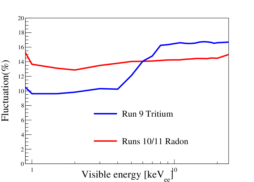
(a) ER

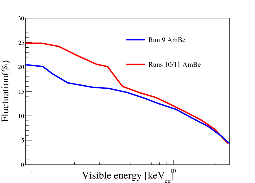
(b) NR

Figure 4: The empirical fluctuation parameter $f$ as a function visible energy for the ER (left) and NR (right) data, both in electron equivalent energy keV_ee

4.2 Model of the detector

The detector model is used to convert $n_{\rm ph}$ and $n_{\rm e}$ to detected $S1$ and $S2$. For the R11410-20 PMTs used in PandaX-II, the double-photoelectron emission probability by the 178 nm scintillation photons $p_{\rm 2pe}$ is measured to be $0.21\pm 0.02$ from the data [6]. Therefore, the number of detected photons ($N_{\rm dph}$) can be simulated as is

$${N_{\rm dph}} ={\rm Binom}(n_{\rm ph},{\rm PDE}/(1+{p_{\rm 2pe}}))$$ (4)

in which ${\rm Binom}(N,p)$ refers to a binomial distribution with $N$ throws and a probability $p$, and $\rm{PDE}/(1+p_{\rm 2pe})$ is the binomial probability to detect a photon. $N_{\rm dph}$ is randomly distributed onto the two arrays of PMTs (55 each) according to the measured top/bottom ratio from the data ($\sim$1:2). Each detected photons are then fluctuated by $p_{\rm 2pe}$, leading to the number of photoelectrons

$${N_{\rm{PE}}} ={N_{\rm dph}}+{\rm Binom}({N_{\rm dph}},p_{\rm 2pe})\,.$$ (5)

$S1$ can be subsequently obtained by applying the single photoelectron (SPE) resolution, modeled as a Gaussian with a $\sigma_{\rm SPE}$ of 33%  [14]

$$S1={{\rm Gaus}(N_{\rm PE}},\sigma_{\rm SPE}\times\sqrt{N_{\rm PE}})\,.$$ (6)

Each $S1$ is required to have at least three hits, with each hit larger than 0.5 PE to simulate the single channel readout threshold and the multiplicity cut in the analysis [6].

Similarly, $S2$ is simulated based on $n_{\rm e}$ by using detector parameters from the data. For each event, the drift time $t_{\rm drift}$ is randomized according to the data distribution, leading to an electron survival probability $s=\exp(-t_{\rm drift}/\tau)$ with the electron lifetime $\tau$ obtained from the data. So at the liquid level, the number of electrons is

$${N_{\rm e}^{{}^{\prime}}}={\rm Binom}(n_{\rm e},s)\,.$$ (7)

Then the number of extracted electron $N_{\rm e}^{{}^{\prime\prime}}$ and $S2$ can be simulated as

$$N_{\rm e}^{{}^{\prime\prime}} ={\rm Binom}(N_{\rm e}^{{}^{\prime}},{\rm EEE})\,,$$ (8)

$$S2 ={\rm Gaus}({N_{\rm e}^{{}^{\prime\prime}}}\times{\rm SEG},\sigma_{\rm SE}\times\sqrt{{N_{\rm e}^{{}^{\prime\prime}}}})\,,$$

in which $\sigma_{\rm SE}\sim 8.3$ PE is the Gaussian width for the single electron signals.

As discussed in Ref. [6], the nonlinearities in $S1$ and $S2$ due to baseline suppression firmware are measured from the data, denoted as $f_{1}(S1)$ and $f_{2}(S2)$. So the detected $S1$ and $S2$ are

$$S1_{d}=S1\times f_{1}\,,S2_{d}=S2\times f_{2}\,.$$ (9)

Finally, the data selection efficiency is parameterized as a Fermi-Dirac function

$$\epsilon(S1_{d})=\frac{1}{1+\exp(\frac{S1_{d}-p_{0}}{p_{1}})}\,,$$ (10)

where $p_{0}$ and $p_{1}$ will be determined by fitting to calibration data. Note that our selection efficiency on $S2$ is expected to be 100$\%$, since the $S2$ selection cut is at 100 PE, significantly higher than the hardware trigger efficiency of 50 PE [15].

4.3 Extraction of parameters in the response model

In this section, the ER and NR response models will be fitted against the calibration data in $S1$ and $S2$ using unbinned likelihood. The systematic uncertainties of the models are quantified by a likelihood ratio approach.

4.3.1 The likelihood function

As an initial approximation, $L_{y}$ can be fitted from the medians of the calibration data distribution as

$$L_{y}^{0}(E_{\rm rec}/L)=\frac{S1}{{\rm PDE}\times E_{\rm rec}/L}\,,$$ (11)

where $E_{\rm rec}$ (Eqn. 1) is the reconstructed energy including all detector effects, and the $\frac{\rm{E_{rec}}}{L}$ is the estimate of $E_{0}$. The true $L_{y}$ can be parameterized as

$$L_{y}(E_{0})=L_{y}^{0}(E_{0})+\sum_{n=0}^{4}c_{n}P_{n}(E_{0})\,,$$ (12)

in which $P_{n}(E_{0})$ is the $n$th order Legendre polynomial functions, and $c_{n}$ can be fitted to data.

For a given model, a two-dimensional probability density function (PDF) in ($S1$,$S2$) is produced with a large statistics simulation described in Secs. 4.1 and 4.2 using the following sets of parameters: a) PDE, EEE and SEG constrained by their Gaussian priors (Table 1), with the anti-correlation between PDE and EEE embedded (see Ref. [16]), b) parameters for $\epsilon(S1_{d})$ in Eqn. 10, with a flat sampling of $p_{0}\in(2,5)$ and $p_{1}\in(0,1)$, respectively, and c) a 4th order Legendre polynomial expansion for $L_{y}$ in Eqn. 12, with $c_{n}$($n=0,1,2,3,4$) uniformly sampled from $-5$ to 5. Other parameters that are independently determined from the data are fixed in the simulation, such as the fluctuation in $n_{\rm e}$, the electron lifetime, $p_{\rm 2pe}$, and the baseline suppression nonlinearities.

To compare the data with the PDF, a standard unbinned log likelihood function is defined in the space of ($S1$,$S2$) as

$$-2\ln\mathcal{L}=\sum_{i=1}^{N}-2\ln(P(S1^{i},S2^{i}))\,\\$$ (13)

in which $P(S1^{i},S2^{i})$ is the probability density for a given calibration data point $i$, and $N$ is the total number of events for each calibration data set.

4.3.2 The best fit and allowable parameter space

An independent parameter scan is carried out to determine the best fit model for each calibration data set. The best fit corresponds to the PDF which gives the minimum $-2\ln\mathcal{L}$. For illustration, the centroids and 90% quantiles of the best fit models from the four data sets are overlaid in Fig. 3, where good agreements with the data are observed.

The parameter space allowable by the calibration data is determined based on the likelihood ratio approach in Ref. [17]. For each set of fixed parameters, 1000 mock data runs are produced with equal but Poisson fluctuated statistics as the calibration data. The test statistic for each mock run is defined as the difference between the log likelihood calculated using this fixed point PDF, and the global minimum value from the parameter scan,

$$\Delta\mathcal{L}=-2{\ln}\mathcal{L}_{\rm fixed}-(-2{\ln}\mathcal{L}_{\rm min})\,.$$ (14)

The distributions of $\Delta\mathcal{L}$ for the mock data generated from the best fit parameters for the four calibration data sets are shown in Fig. 5. The blue dashed regions refer to the 90$\%$ integrals from zero, beyond which the difference between the mock data set and its own PDF becomes less likely. It is verified that the 90% boundary values for $\Delta\mathcal{L}$ at other parameter space points are similar. Therefore, $\Delta\mathcal{L}$ of the real data is tested around the best fit, and the allowable space is defined by the 90$\%$ boundaries in Fig. 5. The corresponding allowable range of distributions in recoil energy, $S1$, and $S2$ are shown in Fig. 6, together with the calibration data, where good agreements are found.

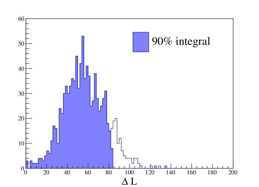
(a) AmBe in Run 9

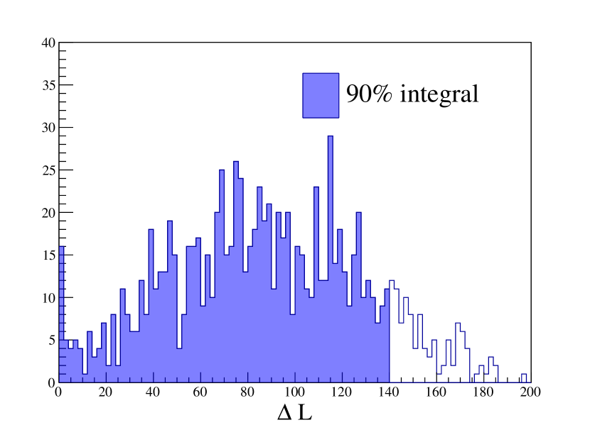
(b) AmBe in Runs 10/11

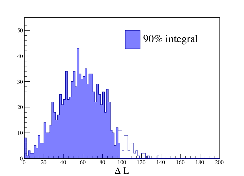
(c) Tritium in Run 9

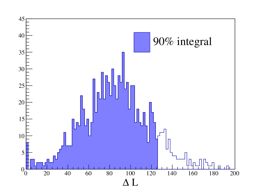
(d) Radon in Runs 10/11

Figure 5: The distribution of $\Delta\mathcal{L}$ for mock calibration data sets generated at the best fit parameter points. The shaded regions indicate the 90% integrals.

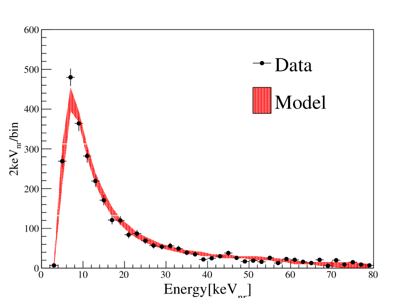
(a) Run 9 AmBe energy

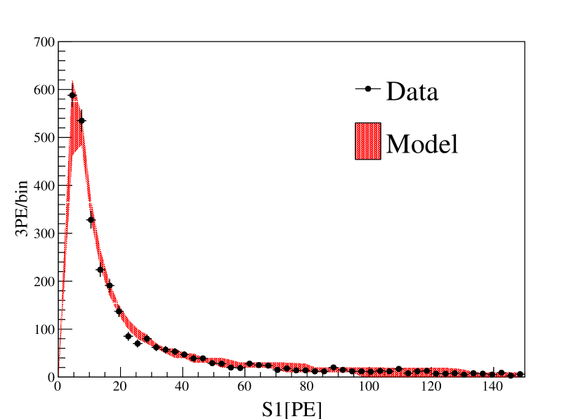
(b) Run 9 AmBe $S1$

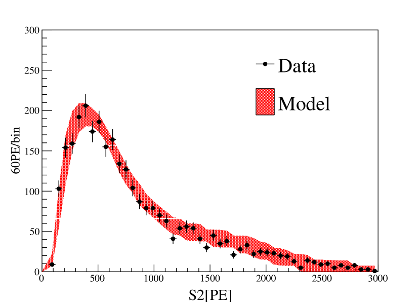
(c) Run 9 AmBe $S2$

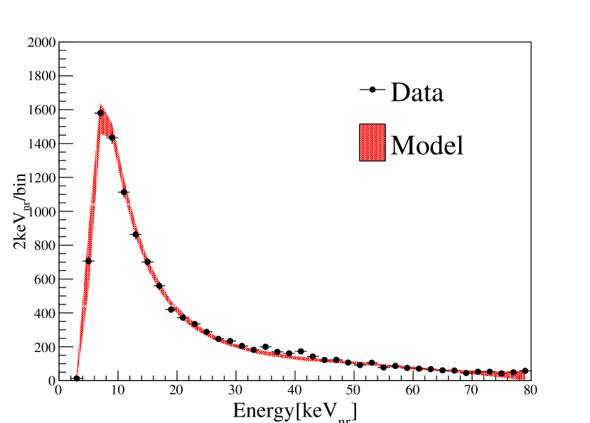
(d) Runs 10/11 AmBe energy

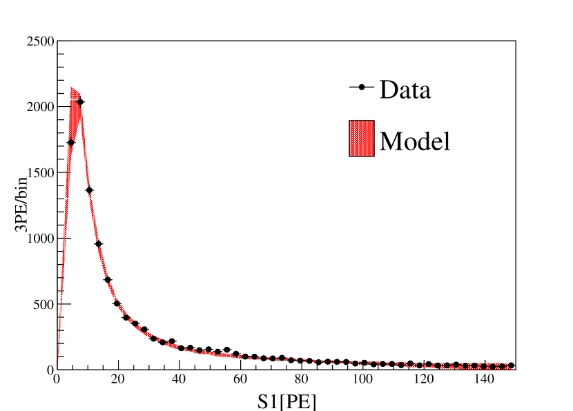
(e) Runs 10/11 AmBe $S1$

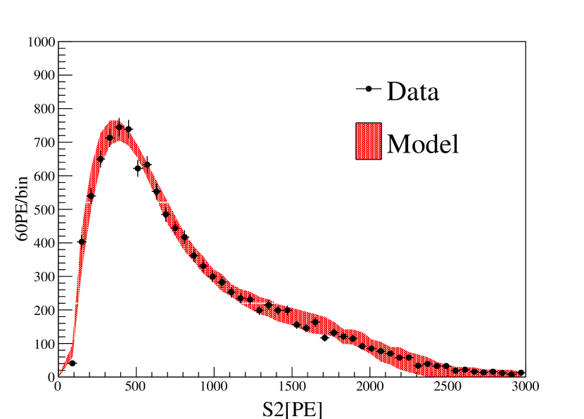
(f) Runs 10/11 AmBe $S2$

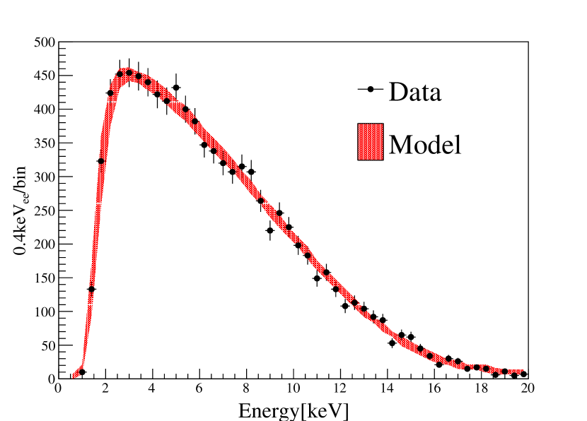
(g) Run 9 CH³T energy

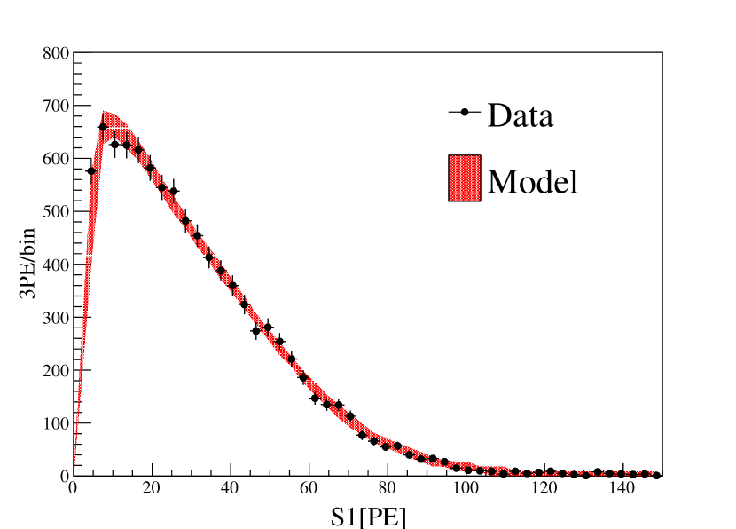
(h) Run 9 CH³T $S1$

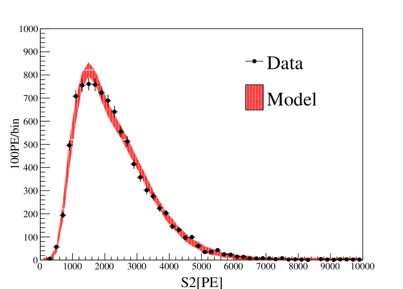
(i) Run 9 CH³T $S2$

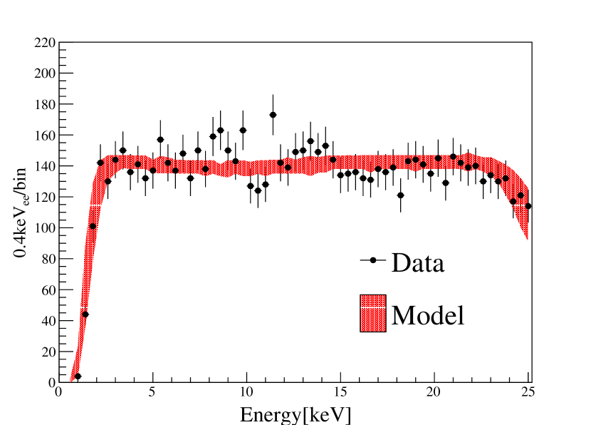
(j) Runs 10/11 ²²⁰Rn energy

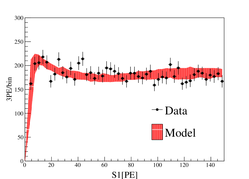
(k) Runs 10/11 ²²⁰Rn $S1$

(l) Runs 10/11 ²²⁰Rn $S2$

Figure 6: The comparison of calibration data (points) and model (shaded bands = 90% allowable) in the recoil energy, $S1$, and $S2$, in Run 9 and Runs 10/11. For the ²²⁰Rn energy distribution (j), the decrease at high energy end is due to the 150 PE $S1$ range cut.

The resulting best fit $Q_{y}$ and $L_{y}$ for the NR and ER events are shown in Fig. 7, overlaid with the world data, as well as the native NEST2.0 predictions [4]. The shaded bands indicate the 90% allowable model space, with uncertainties due to detector parameters and statistics of the calibration data naturally incorporated. Our NR models cover a wide energy range from 4 to 80 keV_nr. At the two drift fields (400 V/cm and 317 V/cm), our best NR models are consistent as expected. For the $Q_{y}$ distribution with recoil energy from 4 to 15 keV_nr, there is significant spread among the world data, in which our $Q_{y}$ appears to be in better agreement with Ref. [18] (Xenon-1T 2019), but lower than the others. The NEST2.0 global fit, presumably mostly driven by data from Ref. [19] (LUX DD), has a higher $Q_{y}$ than ours. The global data agreement improves significantly above 15 keV_nr. $L_{y}$ of our NR models, on the other hand, appear to be in agreement with most of the world data, except some slight tension at above 25 keV_nr with Ref. [20] (Manzur 2010), which bears large uncertainties by itself.

For the ER models, $Q_{y}$ ($L_{y}$) for Run 9 is higher (lower) than that for Runs 10/11. Such a behavior can also be expected since the initial ionized electrons are less likely to be recombined in stronger drift field. Our model at 400 V/cm is in reasonable agreement with Ref. [21] (Xenon100) at similar drift field, but is in some tension with Refs. [22, 23] (neriX 480 V/cm, Lin 424 V/cm). Our $Q_{y}$ ($L_{y}$) at 317 V/cm is generally lower (higher) than the world data, including that from Ref. [19] (LUX) taken at 180 V/cm (and that from Ref. [18] at 81 V/cm, not drawn), as well as the native NEST2.0 predictions. Given the uncertainties in all these measurement, however, more systematic studies and comparisons are warranted.

Regardless of the global comparison, it should be emphasized that for PandaX-II, models determined from in situ calibrations are the most self-consistent models to be used in the dark matter search data. Our best fit models presented here have therefore been adopted in the analysis in Ref. [6].

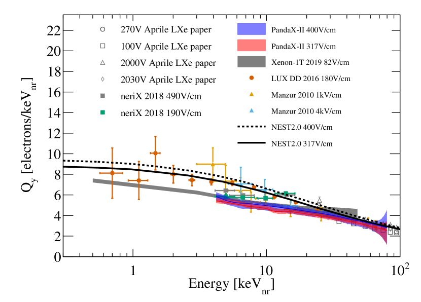
(a) $Q_{y}$ of NR

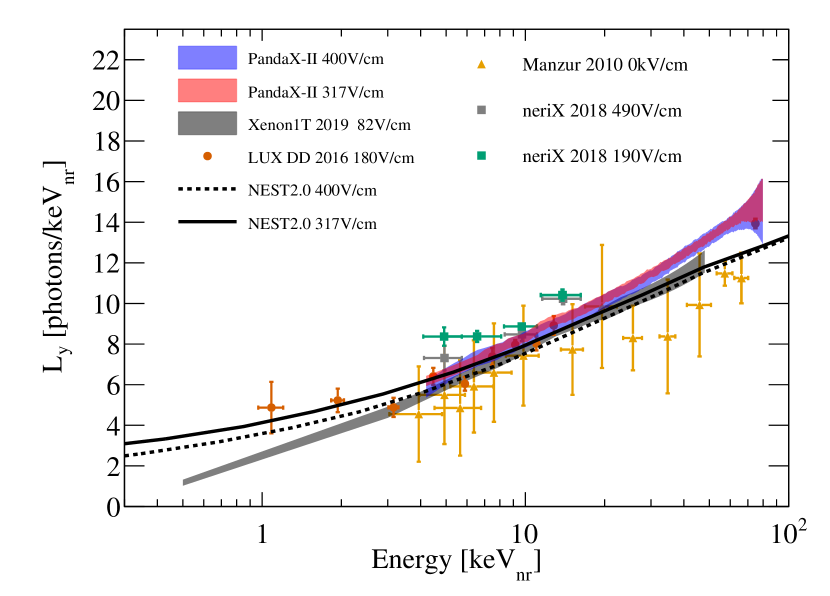
(b) $L_{y}$ of NR

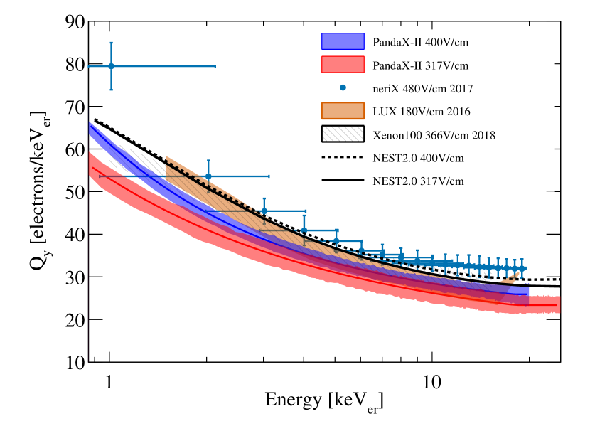
(c) $Q_{y}$ of ER

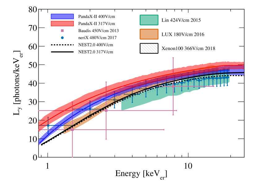
(d) $L_{y}$ of ER

Figure 7: Charge yield $Q_{y}$ (a) and light yield $L_{y}$ (b) of the NR and $Q_{y}$ (c) and $L_{y}$ (d) of the ER obtained from the PandaX-II data: blue=400 V/cm, red=317 V/cm. Overlaid world data include: NR from Refs. [24, 20, 25, 26, 19, 27], and ER from Refs. [28, 23, 7, 22], as indicated in the legend. The native NEST2.0 predictions are drawn in black curves, solid (317 V/cm), and dashed (400 V/cm). The XENON1T responses [18] are not included in the ER figures since the operation field (81 V/cm) is significantly different from the PandaX-II conditions, and for visual clarity.

5 Conclusion

We report the ER and NR responses from the PandaX-II detector based on all calibration data obtained during the operation at two different drift fields (400 V/cm and 317 V/cm). The empirical best fits to the data and model uncertainties are obtained, yielding good agreements between the data and our models. In comparison to those presented in Refs. [29, 16], the models in this work cover the entire PandaX-II data taking period, with a more extend energy range between 4 to 80 keV_nr(NR) and 1 to 25 keV_ee(ER). At the two drift fields, our NR models are in agreement, and our ER models exhibit a relative shift. Both behaviors are consistent with expectation.

Our models are also compared to the world data. Our NR models lie within the large global spread. For the ER response, our model yields a higher (lower) $L_{y}$ ($Q_{y}$) in comparison to most of the world data, indicating some unaccounted systematic uncertainties in our or others’ measurements. These discrepancies encourage continuous calibration effort and further investigations of systematics in the data. Finally, the analysis approach presented here is general and can be applied to similar noble liquid TPC experiments.

6 Acknowledgement

This project is supported in part by a grant from the Ministry of Science and Technology of China (No. 2016YFA0400301), grants from National Science Foundation of China (Nos. 12090060, 11525522, 11775141 and 11755001), and Office of Science and Technology, Shanghai Municipal Government (grant No. 18JC1410200). We thank supports from Double First Class Plan of the Shanghai Jiao Tong University. We also thank the sponsorship from the Chinese Academy of Sciences Center for Excellence in Particle Physics (CCEPP), Hongwen Foundation in Hong Kong, and Tencent Foundation in China. Finally, we thank the CJPL administration and the Yalong River Hydropower Development Company Ltd. for indispensable logistical support and other help.

References

- [1] Andi Tan et al. Dark Matter Search Results from the Commissioning Run of PandaX-II. Phys. Rev., D93(12):122009, 2016.
- [2] E. Aprile et al. The XENON1T Dark Matter Experiment. Eur. Phys. J. C, 77(12):881, 2017.
- [3] D. S. Akerib et al. First results from the lux dark matter experiment at the sanford underground research facility. Phys. Rev. Lett., 112:091303, Mar 2014.
- [4] M. Szydagis et al. https://doi.org/10.5281/zenodo.4283077.
- [5] Yu-Cheng Wu et al. Measurement of Cosmic Ray Flux in China JinPing underground Laboratory. Chin. Phys. C, 37(8):086001, 2013.
- [6] Qiuhong Wang et al. Results of Dark Matter Search using the Full PandaX-II Exposure. 7 2020.
- [7] D. S. Akerib et al. Tritium calibration of the LUX dark matter experiment. Phys. Rev., D93(7):072009, 2016.
- [8] E. Aprile et al. Results from a Calibration of XENON100 Using a Source of Dissolved Radon-220. Phys. Rev. D, 95(7):072008, 2017.
- [9] Wenbo Ma et al. Internal Calibration of the PandaX-II Detector with Radon Gaseous Sources. 6 2020.
- [10] Qiuhong Wang et al. An Improved Evaluation of the Neutron Background in the PandaX-II Experiment. Sci. China Phys. Mech. Astron., 63(3):231011, 2020.
- [11] Xiang Xiao et al. Low-mass dark matter search results from full exposure of the PandaX-I experiment. Phys. Rev., D92(5):052004, 2015.
- [12] M. Szydagis, N. Barry, K. Kazkaz, J. Mock, D. Stolp, M. Sweany, M. Tripathi, S. Uvarov, N. Walsh, and M. Woods. NEST: A Comprehensive Model for Scintillation Yield in Liquid Xenon. JINST, 6:P10002, 2011.
- [13] B. Lenardo, K. Kazkaz, A. Manalaysay, J. Mock, M. Szydagis, and M. Tripathi. A global analysis of light and charge yields in liquid xenon. IEEE Transactions on Nuclear Science, 62(6):3387–3396, 2015.
- [14] Shaoli Li et al. Performance of Photosensors in the PandaX-I Experiment. JINST, 11(02):T02005, 2016.
- [15] Qinyu Wu et al. Update of the trigger system of the PandaX-II experiment. JINST, 12(08):T08004, 2017.
- [16] Xiangyi Cui et al. Dark Matter Results From 54-Ton-Day Exposure of PandaX-II Experiment. Phys. Rev. Lett., 119(18):181302, 2017.
- [17] Glen Cowan, Kyle Cranmer, Eilam Gross, and Ofer Vitells. Asymptotic formulae for likelihood-based tests of new physics. Eur. Phys. J. C, 71:1554, 2011. [Erratum: Eur.Phys.J.C 73, 2501 (2013)].
- [18] E. Aprile et al. XENON1T dark matter data analysis: Signal and background models and statistical inference. Phys. Rev. D, 99(11):112009, 2019.
- [19] D. S. Akerib et al. Low-energy (0.7-74 keV) nuclear recoil calibration of the LUX dark matter experiment using D-D neutron scattering kinematics. 2016.
- [20] A. Manzur, A. Curioni, L. Kastens, D.N. McKinsey, K. Ni, and T. Wongjirad. Scintillation efficiency and ionization yield of liquid xenon for mono-energetic nuclear recoils down to 4 keV. Phys. Rev. C, 81:025808, 2010.
- [21] E. Aprile et al. Signal Yields of keV Electronic Recoils and Their Discrimination from Nuclear Recoils in Liquid Xenon. Phys. Rev. D, 97(9):092007, 2018.
- [22] L.W. Goetzke, E. Aprile, M. Anthony, G. Plante, and M. Weber. Measurement of light and charge yield of low-energy electronic recoils in liquid xenon. Phys. Rev. D, 96(10):103007, 2017.
- [23] Qing Lin, Jialing Fei, Fei Gao, Jie Hu, Yuehuan Wei, Xiang Xiao, Hongwei Wang, and Kaixuan Ni. Scintillation and ionization responses of liquid xenon to low energy electronic and nuclear recoils at drift fields from 236 V/cm to 3.93 kV/cm. Phys. Rev. D, 92(3):032005, 2015.
- [24] E. Aprile, C.E. Dahl, L. DeViveiros, R. Gaitskell, K.L. Giboni, J. Kwong, P. Majewski, Kaixuan Ni, T. Shutt, and M. Yamashita. Simultaneous measurement of ionization and scintillation from nuclear recoils in liquid xenon as target for a dark matter experiment. Phys. Rev. Lett., 97:081302, 2006.
- [25] Peter Sorensen. A coherent understanding of low-energy nuclear recoils in liquid xenon. JCAP, 09:033, 2010.
- [26] E. Aprile et al. Response of the XENON100 Dark Matter Detector to Nuclear Recoils. Phys. Rev. D, 88:012006, 2013.
- [27] E. Aprile, M. Anthony, Q. Lin, Z. Greene, P. De Perio, F. Gao, J. Howlett, G. Plante, Y. Zhang, and T. Zhu. Simultaneous measurement of the light and charge response of liquid xenon to low-energy nuclear recoils at multiple electric fields. Phys. Rev. D, 98(11):112003, 2018.
- [28] Laura Baudis, Hrvoje Dujmovic, Christopher Geis, Andreas James, Alexander Kish, Aaron Manalaysay, Teresa Marrodan Undagoitia, and Marc Schumann. Response of liquid xenon to Compton electrons down to 1.5 keV. Phys. Rev. D, 87(11):115015, 2013.
- [29] Andi Tan et al. Dark Matter Results from First 98.7 Days of Data from the PandaX-II Experiment. Phys. Rev. Lett., 117(12):121303, 2016.