An Enhanced Adversarial Network with Combined Latent Features for Spatio-Temporal Facial Affect Estimation in the Wild

Abstract

Affective Computing has recently attracted the attention of the research community, due to its numerous applications in diverse areas. In this context, the emergence of video-based data allows to enrich the widely used spatial features with the inclusion of temporal information. However, such spatio-temporal modelling often results in very high-dimensional feature spaces and large volumes of data, making training difficult and time consuming. This paper addresses these shortcomings by proposing a novel model that efficiently extracts both spatial and temporal features of the data by means of its enhanced temporal modelling based on latent features. Our proposed model consists of three major networks, coined Generator, Discriminator, and Combiner, which are trained in an adversarial setting combined with curriculum learning to enable our adaptive attention modules. In our experiments, we show the effectiveness of our approach by reporting our competitive results on both the AFEW-VA and SEWA datasets, suggesting that temporal modelling improves the affect estimates both in qualitative and quantitative terms. Furthermore, we find that the inclusion of attention mechanisms leads to the highest accuracy improvements, as its weights seem to correlate well with the appearance of facial movements, both in terms of temporal localisation and intensity. Finally, we observe the sequence length of around 160 ms to be the optimum one for temporal modelling, which is consistent with other relevant findings utilising similar lengths.

1 INTRODUCTION

Affective Computing has recently attracted the attention of the research community, due to its numerous applications in diverse areas which include education [Duo and Song, 2010] or healthcare [Liu et al., 2008], among others. The growing availability of affect-related datasets, such as AFEW-VA [Kossaifi et al., 2017] and the recently introduced SEWA [Kossaifi et al., 2019] database enable the rapid development of deep learning-based techniques, which currently hold the state of the art.

Further, the emergence of video-based data allows to enrich the widely used spatial features with the inclusion of temporal information. To this end, several authors have explored the use of long-short term memory (LSTM) recurrent neural networks (RNNs) [Tellamekala and Valstar, 2019, Ma et al., 2019], endowed also with attention mechanisms  [Luong et al., 2015, Li et al., 2020, Xiaohua et al., 2019]. However, such spatio-temporal modelling often results in very high-dimensional feature spaces and large volumes of data, making training difficult and time consuming. Moreover, it has been shown that the sequence length considered during training can be a decisive factor for successful temporal modelling [Kossaifi et al., 2017, Xia et al., 2020, Farhadi and Fox, 2018, Aspandi et al., 2019b], and yet a detailed study of this aspect is lacking in the field.

This paper addresses both the lack of incorporation and analysis of temporal modelling on affective analysis. We propose a novel model which can be efficiently used to extract both spatial and temporal features of the data by means of its enhanced temporal modelling based on latent features. We do so by incorporating three major networks, coined Generator, Discriminator, and Combiner, which are trained in an adversarial setting to estimate the affect domains of Valence (V) and Arousal (A). Furthermore, we capitalise on these latent features to enable temporal modelling using LSTM RNNs, which we train progressively using curriculum learning enhanced with adaptive attention. Specifically, the contributions of this paper are as follows:

1. We upgrade the standard adversarial setting, consisting of a Generator and a Discriminator, with a third network that combines the features from these networks, which are modified accordingly. This yields features that combine the latent space from the autoencoder-based Generator and a V-A Quadrant estimate produced by the modified Discriminator, resulting in a compact but meaningful representation that helps reduce the training complexity.

2. We propose the use of curriculum learning to enable analysis and optimisation of the temporal modelling length.

3. We incorporate dynamic attention to further enhance our model estimates and show its effectiveness by reporting state of the art accuracy on both the AFEW-VA and SEWA datasets.

2 RELATED WORK

Affective Computing started by exploiting the use of classical machine learning techniques to enable automatic affect estimation. Examples of early approaches include partial least squares regression [Povolny et al., 2016], and support vector machines [Nicolaou et al., 2011]. Subsequently, to further progress the investigations in this field, the development of larger and bigger datasets was addressed. Several datasets have been introduced so far, starting with SEMAINE [McKeown et al., 2010], AFEW-VA [Kossaifi et al., 2017], RECOLA [Ringeval et al., 2013], OMG [Barros et al., 2018], AffectNet [Mollahosseini et al., 2015], and more recently SEWA [Kossaifi et al., 2019], aff-wild [Kollias et al., 2019, Zafeiriou et al., 2017], and  aff-wild2[Kollias and Zafeiriou, 2019, Kollias et al., 2020]. Furthermore, the V-A labels have become the standard emotional dimensions over time, as opposed to hard emotion labels, given their continuous nature [Kossaifi et al., 2017, Kossaifi et al., 2019].

Throughout the last few years, models based on Deep Learning have emerged and currently hold the state of the art in the context of affective analysis, given their ability to learn from large scale data. A recent example along this line is the work from Mitenkova et al. [Mitenkova et al., 2019], who introduce tensor modelling for affect estimations by using spatial features. In their work, they use tucker tensor regression optimised by means of deep gradient methods, thus allowing to preserve the structure of the data and reduce the number of parameters. Other works, such as [Handrich et al., 2020], adopt the multi-task approach to simultaneously address face detection and affective states prediction. Specifically, they use YOLO-based CNN models [Huang et al., 2018] to estimate the facial locations alongside V-A values through their proposed combined losses. As such, their models are able to incorporate the characteristics of facial attributes and estimate their relevance to affect inferences.

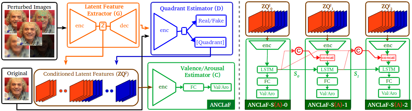
Figure 1: Schematic representation of our Full ANCLaF Networks. Left is our base model, which consists of three networks jointly trained in an adversarial setting: Latent Feature Extractor (G), Quadrant Estimator (D), and Valence Arousal Estimator (C). On the right, we see our network endowed with sequence modelling (ANCLaF-S) and attention mechanism (ANCLaF-SA).

The recent growth of video-based datasets has encouraged the inclusion of temporal modelling, which has shown to improve models’ training [Xie et al., 2016, Cootes et al., 1998]. Relevant examples in Affective Computing include the works of Tellamekala et al. [Tellamekala and Valstar, 2019] and Ma et al. [Ma et al., 2019]. In their work, Tellamekala et al. [Tellamekala and Valstar, 2019] enforce temporal coherency and smoothness aspects on their feature representation by constraining the differences between adjacent frames, while Ma et al. resort to the utilisation of LSTM RNNs with residual connections applied to multi-modal data. Furthermore, the use of attention has also been recently explored by Xiaohua et al. [Xiaohua et al., 2019] and Li et al. [Li et al., 2020]. Xiahoua et al. adopt multi-stage attention, which involves both spatial and temporal attention, on their facial based affect estimations. Meanwhile, using spectrogram data as input, Li et al. propose a deep network that utilises an attention mechanism [Luong et al., 2015] on top of their LSTM networks to predict the affective states.

Unfortunately, to our knowledge, all previous works involving temporal modelling on affective computing miss one important aspect of the analysis: the involved sequence length in their training. While the specified length of temporal modelling has been shown to affect the final results on other related facial analysis tasks [Kossaifi et al., 2017, Xia et al., 2020, Farhadi and Fox, 2018, Aspandi et al., 2019b], the computational cost required to train large spatio-temporal models hampers one to address such analysis. However, these problems could be mitigated by: 1) the use of progressive sequence learning to permit step-wise observations of various sequence lengths; this approach has been shown in the recent work of [Aspandi et al., 2019b] on facial landmark estimations, which uses curriculum learning enabling more robust training analysis and tuning of the temporal length; 2) the use of reduced feature sizes, enabling more efficient training process [Comas et al., 2020]; this has been explored in the affective computing field by the recent works such as [Aspandi et al., 2020], which uses generative modelling to extract a latent space of representative features. These two aspects have inspired us to propose the combined models presented in this work, as explained in the next section.

3 METHODOLOGY

Figure 1 shows the overview of our proposed models, which consist of three networks: a Latent Feature Extractor (acting as Generator, G), a Quadrant Estimator (or Discriminator, D), and a Valence/Arousal Estimator (or Combiner, C). Given input image I which contains the facial area, both G and D will be responsible to learn low dimensional features that the combiner will use to estimate the associated Valence (V) and Arousal (A) state $\theta$. The architecture of both the G and D networks follows the recent work from [Aspandi et al., 2020], and we propose to use LSTM enhanced with attention to create our C network. We proposed two main architecture variants: the ANCLaF network (left part of Figure 1), which uses single images as input and estimates V and A values independently for each frame, and ANCLaF-S and ANCLaF-SA (right part of Figure 1) that uses sequences of latent features extracted from $n$ frames as input, and utilises LSTM RNNs for the inference (-S), optionally combined with internal attention layers (-SA).

3.1 Adversarial Network with Combined Latent Features (ANCLaF)

The pipeline of our base model ANCLaF starts with the G network. It receives either the original input image I, or a distorted version of it, $\tilde{I}$, as detailed in [Aspandi et al., 2019c, Aspandi et al., 2019a]. It simultaneously produces the cleaned reconstruction of the input image $\hat{I}$ and a 2D latent representation that will be used as features ($\mathbb{Z}$):

$$G(I)_{\varPhi^{G}}=dec_{\varPhi^{G}}(enc_{\varPhi^{G}}(I))\,with\,\mathbb{Z}^{I}\approx enc_{\varPhi^{G}}(I),$$ (1)

where $\varPhi$ are the parameters of the respective networks, $enc$ and $dec$ are the encoder and decoder, respectively. Subsequently, the D network receives $\hat{I}$ and tries to estimate whether it was obtained from a true or fake example (namely, original or distorted input image), as well as a rough estimate of the affective state. In contrast with the formulation in [Aspandi et al., 2020], in which D targets directly the intensity of V and A, we propose to base the estimated affect on the circumplex quadrant ($\mathbb{Q}$) [Russell, 1980] which discretises emotions along the valence and arousal dimensions (four quadrants). This, in turn, reduces the training complexity. Thus, letting FC stand for fully connected layer:

$$D(I)_{\varPhi^{D}}=FC_{\varPhi^{D}}(enc_{\varPhi^{D}}(I))\Rightarrow\mathbb{Q}^{I}\ and\ \{0,1\}.$$ (2)

Then, $\mathbb{Q}$ is used to condition the extracted latent features $\mathbb{Z}$ through layer-wise concatenation, which we call $\mathbb{ZQ}$ [Dai et al., 2017, Ye et al., 2018]. Given these conditioned latent features, the C network performs the final stage of affect estimation, producing refined predictions of both V and A [Lv et al., 2017, Triantafyllidou and Tefas, 2016, Aspandi et al., 2019b]. Thus, if $\hat{\theta}$ denote the estimated V and A:

$$\begin{split}ANCLaF(I)&=C_{\varPhi^{C}}([G_{\varPhi^{G}}(I);D_{\varPhi^{D}}(G_{\varPhi^{G}}(I))])\\ &=C_{\varPhi^{C}}([\mathbb{Z}^{I};\mathbb{Q}^{I}])\\ &=FC_{\varPhi^{C}}(enc_{\varPhi^{C}}([\mathbb{Z}^{I};\mathbb{Q}^{I}]))\Rightarrow\hat{\theta}^{I}_{ANCLaF}.\\ \end{split}$$ (3)

3.2 Attention Enhanced Sequence Latent Affect Networks

We propose two sequence-based variants of our models: ANCLaF-S and -SA. Both of them use the combined features extracted by the G and D networks $\mathbb{ZQ}$, which are fed to LSTM networks to allow for temporal modelling [Hochreiter and Schmidhuber, 1997] and complemented with an FC layer to produce the final estimates. These networks are trained using curriculum learning [Bengio et al., 2009, Farhadi and Fox, 2018, Aspandi et al., 2019b], in which the number of frames is progressively increased, allowing more throughout analysis of the training progress. Moreover, the training outcome for a given length facilitates the subsequent training of larger sequences [Farhadi and Fox, 2018]. In this work, we considered a series of 2, 4, 8, 16, and 32 successive frames ($\textsc{N}=\{2,4,8,6,32\}$) for both training and inference stages. Depending on the number of frames to take into account (n), we use ANCLaF-S-n and ANCLaF-SA-n to name the respective variants of both ANCLaF-S and ANCLaF-SA networks. Lastly, the main difference between the two sequence models is that ANCLaF-SA also includes internal attentional modelling using the current and previous internal states from the LSTM layers. Thus, V-A predictions of ANCLaF-S-n are:

$$\forall n\in\textsc{N}\,,\,ANCLaF\textnormal{-}S\textnormal{-}n(I_{n}),h_{n}=\\ FC_{\varPhi^{C}}(LSTM_{\varPhi^{C}}([Z^{I}_{n},Q^{I}_{n}],h_{n-1}))\\ \Rightarrow FC_{\varPhi^{C}}(LSTM_{\varPhi^{C}}(\mathbb{ZQ}^{I}_{n},h_{n-1})),$$ (4)

where LSTM is the Long Short Term Memory network [Hochreiter and Schmidhuber, 1997], and $h_{n}$ are LSTM states (h) after n successive frames. Built upon $ANCLaF\textnormal{-}SA$, we further use attention modelling [Luong et al., 2015] to enable adaptive weights on model inferences by calculating the context vectors ($\mathbb{C}$) that summarise the importance of each previous state $h$. Differently from the original method, however, here, we also propose to include both the LSTM inner state (c) and outgoing states (h) [Kim et al., 2018] to provide the full previous information, and also to adapt these techniques to only consider n previous states following our curriculum learning approach. Hence, given the combined LSTM states at frame $t$, denoted ($S_{t}=[c_{t},h_{t}]$), and $n$ previous states ($\bar{S}$), the alignment score is calculated as:

$$\mbox{\boldmath{$a$}}_{n}(t) =\operatorname{align}(\mbox{\boldmath{$S$}}_{t},\mbox{\boldmath{$\bar{S}$}}_{t})\,,\,with\,S_{x}=[h_{x};c_{x}]$$ (5)

$$=\frac{\exp\left(\mbox{\boldmath{$W_{a}$}}[\mbox{\boldmath{$S$}}_{t}^{\top};\mbox{\boldmath{$\bar{S}$}}_{n}]\right)}{\sum_{N^{\prime}}\exp\left(\mbox{\boldmath{$W_{a}$}}[\mbox{\boldmath{$S$}}_{t}^{\top};\mbox{\boldmath{$\bar{S}$}}_{n^{\prime}}]\right)}.$$

Then, the location-based function computes the alignment scores from the previous states ($\bar{S}$):

$$\mbox{\boldmath{$a$}}_{n}=\operatorname{softmax}(\mbox{\boldmath{$W_{a}$}}\bar{S}).$$ (6)

Given the alignment vector, it is used to compute the context vector $\mathbb{C}_{t}$ as the weighted average over the considered $n$ previous hidden states:

$$\mathbb{C}_{t}=\frac{\sum_{n}a_{n}\odot S_{n}}{n}$$ (7)

Finally, the context vector is concatenated with the current $\mathbb{ZQ}$ to be used as input to the C network pipeline:

$$\forall n\in\textsc{N}\,,\,ANCLaF\textnormal{-}SA\textnormal{-}n(I_{n}),h_{n}=\\ FC_{\varPhi^{C}}(LSTM_{\varPhi^{C}}([\mathbb{C}_{n};\mathbb{ZQ}^{I}_{n}],h_{n-1})).$$ (8)

3.3 Training Losses

We use the modified adversarial training from [Aspandi et al., 2020] to train both the G and D networks, and incorporate the training of the C network by providing the latter with the features extracted from both the G and D nets on the fly. With this setup, we allow C to benefit from the improved quality of the features extracted by G and D as their training progresses. The equations for the modified adversarial training of these three networks are:

$$\begin{split}\mathcal{L}_{adv}=&\thinspace{\mathbb{E}}_{I}\left[\log{{D}(I)}\right]\>\>+\\ &\thinspace{\mathbb{E}}_{I}[\log{(1-{D}(G(\tilde{I})))}+\thinspace{\mathbb{E}}_{afc}[C(I),\theta_{I}].\end{split}$$ (9)

We use similar ${L}_{afc}$ losses as in [Aspandi et al., 2020], which incorporates multiple affect metrics: Rooted Mean Square Error (RMSE) (Eq. 11), Correlation(COR) (Eq. 12), Concordance Correlation Coefficients (CCC) (Eq. 13), and [Kossaifi et al., 2017] with the addition of Intra-class Correlation Coefficient (ICC)[Kossaifi et al., 2019]. Thus, with {$\hat{\theta}$,$\theta$} as the predicted and the ground truth V-A values, the $\mathcal{L}_{afc}$ is defined as follows:

$$\mathbb{E}_{afc}=\sum_{i=1}^{F}\frac{f_{i}}{F}(\mathcal{L}_{RMSE}+\mathcal{L}_{COR}+\mathcal{L}_{CCC}+\mathcal{L}_{ICC})$$ (10)

$$\mathcal{L}_{RMSE}=\sqrt{\frac{1}{n}\sum_{i=1}^{n}(\hat{\theta_{i}}-\theta_{i})^{2}},\\$$ (11)

$$\mathcal{L}_{COR}=\frac{\mathbb{E}[(\hat{\theta}-\hat{\mu_{\theta}})-(\theta-\mu_{\theta})]}{\sigma_{\hat{\theta}}\sigma_{\theta}}\\$$ (12)

$$\mathcal{L}_{CCC}=2x\frac{\mathbb{E}[(\hat{\theta}-\hat{\mu_{\theta}})-(\theta-\mu_{\theta})]}{\sigma_{\hat{\theta}}^{2}+\sigma_{\theta}^{2}+(\mu_{\hat{\theta}}-\mu_{\theta})^{2}}$$ (13)

$$\mathcal{L}_{ICC}=2x\frac{\mathbb{E}[(\hat{\theta}-\hat{\mu_{\theta}})-(\theta-\mu_{\theta})]}{\sigma_{\hat{\theta}}^{2}+\sigma_{\theta}^{2}},$$ (14)

where $f_{i}$ is the total number of instances of discrete V-A classes $i$, and $F$ is a normalisation factor [Aspandi et al., 2019a] for the total V-A classes (discretised by a value of 10). This normalisation factor is crucial in cases of large imbalance in the number of instances per class, like in the AFEW-VA dataset (see Section 4.1).

3.4 Model Training

We use both the AFEW [Kossaifi et al., 2017] and SEWA [Kossaifi et al., 2019] datasets to train all our model variants, by following their original subject-independent protocol (5-fold cross validation). We conducted two training stages for each of our proposed models. Firstly, we trained the G, D, and C networks simultaneously using adversarial loss as indicated in Equation 9. This training stage produced our baseline results without any sequential modelling, and conditional latent features $\mathbb{ZQ}$ to be used for the next stages of ANCLaF-S(A) Training.

In the second stage, The training of both ANCLaF-S and ANCLaF-SA was performed using the combined latent and quadrant features, under the previously defined curriculum learning scheme. We progressively train our ANCLaF-S models from 2, 4, 8, 16 to 32 steps of temporal modelling with multi-stage transfer learning [Christodoulidis et al., 2016]. Subsequently, we add our proposed attention mechanism to the pre-trained ANCLaF-S models, thus obtaining our ANCLaF-SA models. In both cases, we optimise the affect loss defined in Equation 10 with the same experimental settings used to train ANCLaF.

We need to note that our combined training setup translates to more than 100 experiments in total. Hence, the use of latent features (known as a good choice to achieve reduced dimensionality representations) is critical to speed up our training process and make our experiments feasible. We observed a saving up to 1 : 4 of the original times during training each of our models by using the extracted latent features, with respect to using the original image (around 12 hours versus 2 days) on a single NVIDIA Titan X GPU. Full definitions of our models can be found in the respective online source code.

4 EXPERIMENTS AND RESULTS

4.1 Datasets and Experiment Settings

To quantify the impact of our temporal modelling, we opted to use two of the most popular and accessible video datasets available: Acted Facial Expressions in the Wild (AFEW-VA)[Kossaifi et al., 2017] and Automatic Sentiment Analysis in the Wild (SEWA)[Kossaifi et al., 2019]. On the one hand, AFEW-VA has more individual examples (600 versus 538) than SEWA, however, the latter has more frame examples, more contextual information (such as subject, id of the associated culture) and is more balanced in terms of V-A labels [Mitenkova et al., 2019]. Furthermore, both datasets contain in the wild situations, enabling real time model evaluations. Finally, the labels provided are in the form of continuous V-A values, together with additional facial landmark locations that we refined further using other external models [Aspandi et al., 2019b] to obtain more stable detection of the facial area.

In each experiment, we provide the results from all variants of our models to highlight the contribution of each module: first, we evaluate the ANCLaF model, which operates by exclusively using the latent features extracted on each frame ($\mathbb{ZQ}$) without any temporal modelling. Then, we provide results from both ANCLaF-S and ANCLaF-SA, which incorporate temporal modelling (and attention in the case of -SA). We report both RMSE and COR results, on both datasets, adding also ICC and CCC metrics for the AFEW-VA and SEWA datasets, respectively, to facilitate quantitative analysis to other results reported in the literature. Finally, for fair comparisons, we compare our models against external results which followed similar experimental protocols, i. e., using exclusively this dataset in their training stage.

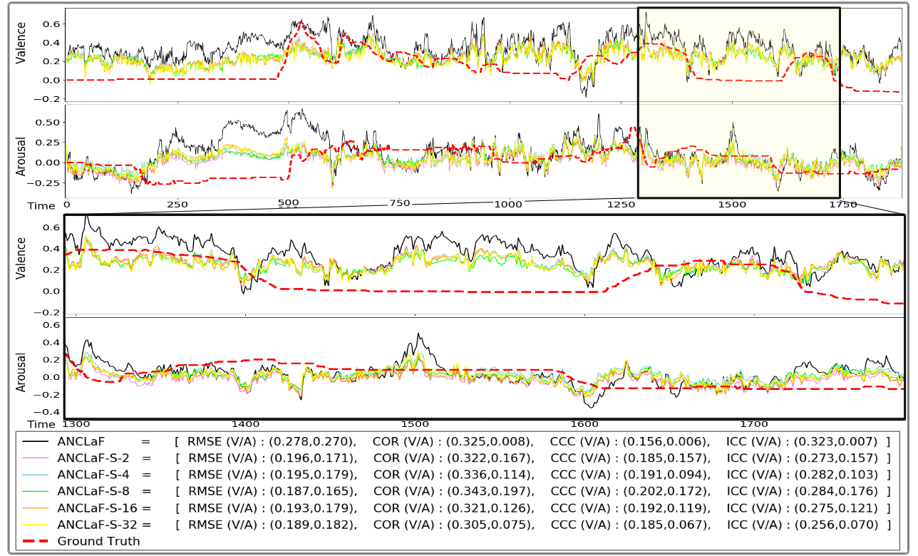
Figure 2: Analysis of prediction results from a single frame (ANCLaF) and from multiple frames with temporal modelling (ANCLaF-S-n). Top: the overview of the overall results; Bottom:, a closer look at the prediction results.

4.2 Comparative Results

Table 1 and table 2 provide the full comparisons of our proposed models against other reported results for both the AFEW-VA and SEWA datasets, respectively. We can identify several findings based on these results: Firstly, that our base ANCLaF model, relying on a single image at a time, can produce quite competitive accuracy compared to other results from the literature. Furthermore, its accuracy is also higher than the results from the original AEG-CD-SZ models in which it is based upon [Aspandi et al., 2020], as shown by its higher accuracy on the SEWA datasets, especially for Valence. This may indicate its better processing capabilities of the visual features, considering that AEG-CD-SZ also incorporates audio features, which in a way also explains its higher accuracy on the prediction of Arousal.

Table 1: Quantitative comparisons on the AFEW-VA dataset.

Model	RMSE$\;\downarrow$			COR$\;\uparrow$			ICC$\;\uparrow$
	VAL	ARO	AVG	VAL	ARO	AVG	VAL	ARO	AVG
Baseline [Kossaifi et al., 2017]	2.680	2.275	2.478	0.407	0.450	0.429	0.290	0.356	0.323
Coherent[Tellamekala and Valstar, 2019]	-	-	-	0.293	0.426	0.360	-	-
Simul [Handrich et al., 2020]	2.600	2.500	2.550	0.390	0.290	0.340	0.320	0.210	0.265
ANCLaF	2.682	2.344	2.513	0.306	0.399	0.353	0.219	0.309	0.264
ANCLaF-S-2	2.675	2.295	2.485	0.314	0.410	0.362	0.236	0.296	0.266
ANCLaF-S-4	2.654	2.279	2.467	0.303	0.420	0.361	0.224	0.307	0.266
ANCLaF-S-8	2.595	2.202	2.398	0.328	0.425	0.377	0.272	0.344	0.308
ANCLaF-S-16	2.617	2.292	2.454	0.302	0.401	0.351	0.224	0.299	0.261
ANCLaF-S-32	2.568	2.328	2.448	0.288	0.405	0.346	0.214	0.304	0.259
ANCLaF-S-AVG	2.622	2.279	2.450	0.307	0.412	0.360	0.234	0.310	0.272
ANCLaF-SA-2	2.540	2.241	2.390	0.373	0.454	0.413	0.291	0.353	0.322
ANCLaF-SA-4	2.586	2.260	2.423	0.386	0.445	0.415	0.302	0.342	0.322
ANCLaF-SA-8	2.481	2.239	2.360	0.371	0.467	0.419	0.294	0.367	0.331
ANCLaF-SA-16	2.601	2.225	2.413	0.377	0.467	0.422	0.294	0.363	0.328
ANCLaF-SA-32	2.581	2.256	2.419	0.361	0.436	0.399	0.270	0.332	0.301
ANCLaF-SA-AVG	2.558	2.244	2.401	0.373	0.454	0.414	0.290	0.352	0.321

Table 2: Quantitative comparisons on the SEWA dataset.

Model	RMSE $\;\downarrow$			COR $\;\uparrow$			CCC $\;\uparrow$
	VAL	ARO	AVG	VAL	ARO	AVG	VAL	ARO	AVG
Baseline [Kossaifi et al., 2019]	-	-	-	0.350	0.350	0.350	0.350	0.290	0.320
Tensor [Mitenkova et al., 2019]	0.334	0.380	0.357	0.503	0.439	0.471	0.469	0.392	0.431
AEG-CD-SZ[Aspandi et al., 2020]	0.323	0.350	0.337	0.442	0.478	0.460	0.405	0.430	0.418
ANCLaF	0.354	0.347	0.351	0.530	0.395	0.462	0.492	0.364	0.428
ANCLaF-S-2	0.349	0.345	0.347	0.533	0.396	0.464	0.503	0.368	0.436
ANCLaF-S-4	0.344	0.336	0.340	0.536	0.403	0.469	0.510	0.382	0.446
ANCLaF-S-8	0.341	0.339	0.340	0.538	0.404	0.471	0.514	0.381	0.448
ANCLaF-S-16	0.354	0.344	0.349	0.527	0.395	0.461	0.490	0.369	0.429
ANCLaF-S-32	0.353	0.346	0.349	0.527	0.396	0.461	0.494	0.368	0.431
ANCLaF-S-AVG	0.348	0.342	0.345	0.532	0.399	0.465	0.502	0.374	0.438
ANCLaF-SA-2	0.343	0.333	0.338	0.545	0.420	0.482	0.509	0.390	0.449
ANCLaF-SA-4	0.336	0.328	0.332	0.550	0.429	0.490	0.526	0.399	0.463
ANCLaF-SA-8	0.336	0.332	0.334	0.558	0.424	0.491	0.529	0.405	0.467
ANCLaF-SA-16	0.334	0.331	0.332	0.556	0.421	0.488	0.528	0.393	0.461
ANCLaF-SA-32	0.336	0.362	0.349	0.550	0.418	0.484	0.513	0.389	0.451
ANCLaF-SA-AVG	0.337	0.337	0.337	0.552	0.422	0.488	0.521	0.395	0.458

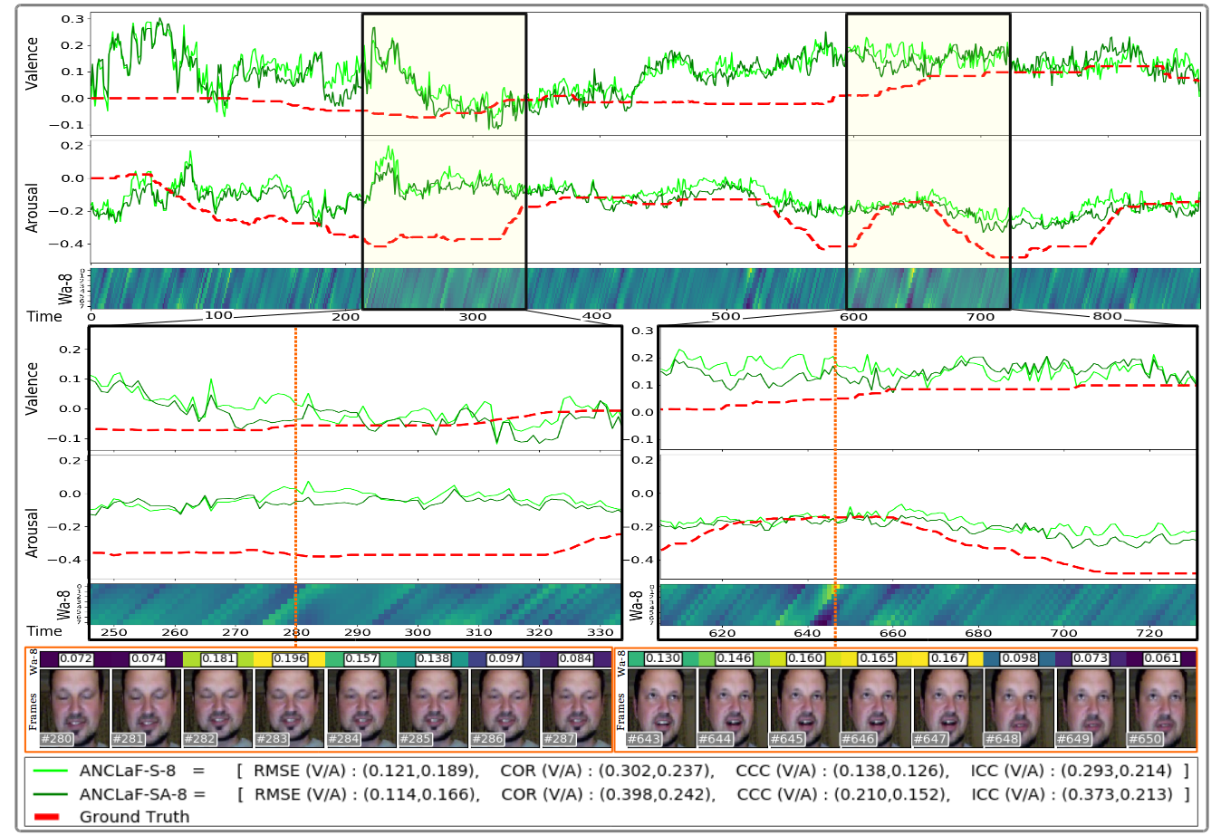
Figure 3: Analysis of the attention impact on the prediction results of our sequence modelling (results from ANCLaF-S-8 and ANCLaF-SA-8, which correspond to the best ANCLaF-S and ANCLaF-SA models, respectively). Top: overview of the overall results; Bottom: two examples of a closer view on the prediction graph. The column Wa-8 shows the attention weights learnt for the eight considered frames.

Secondly, we notice a slight accuracy improvement when our models incorporate sequence modelling (ANCLaF-S), especially in terms of correlations, namely, concordeance corelation coefficient (CCC), and ICC. This finding demonstrates the benefit of the temporal modelling, yielding more stable results than those achieved by ANCLaF (cf.  Section 4.3). However, even though the overall accuracy of ANCLaF-S is better than that of ANCLaF (and quite comparable to other state of the art models), the improvement can be considered modest, especially if we compare it with the improvement achieved when we include attention in our models. Indeed, we can see that our ANCLaF-SA outperforms almost all compared models across the different affect metrics. These findings suggest that the plain utilisation of LSTMs may not be enough to attain a considerable and substantial increase of accuracy [Schmitt et al., 2019], justifying the inclusion of the attention mechanism in our approach.

Thirdly, we further observe a noticeable trend of steady increase in accuracy from the predictions of both ANCLaF-S and ANCLaF-SA as the number of considered frames grows from 2 to 8, and then it plateaus (or even worsens a bit) as $n$ continues to increase. This trend suggests that generally, a medium sequence length (between 4 to 16 frames) is optimal to produce more accurate predictions and that too short and too long sequences degrade temporal modelling. This finding is quite consistent with those from [Aspandi et al., 2019b], indicating the importance of progressive learning, which allows us to analyse and choose the optimal sequence length during training. Lastly, this sequence length selection may also impact the context vector along with its weights learnt in our attentional module, which explains why a similar trend was observed in the results from these models (see Section 4.4 for more details).

4.3 Analysis of the Impact of Sequence Modelling

Figure 2 shows an example of V-A predictions for ANCLaF and ANCLaF-S-n, together with the ground-truth annotations. Specifically, in the top part, we can see the predicted affect states from our models that, in general, are quite related to the ground truth values. However, we notice that the results of our sequence based models are more accurate than their non-sequential counterparts. We can also see that the the predicted values from ANCLaF are quite sparse, thus, quite unstable compared to ANCLAF-S, which explains its lower COR, CCC, and ICC values. Our sequence modelling, on the other hand, is able to create smooth predictions with higher overall accuracy.

On the bottom part of the figure, showing a magnified portion of the same example, we further notice that the results for all ANCLaF-S-n are quite similar, with those from ANCLaF-S-8 showing the highest resemblance to the ground-truth. Thus, inclusion of too short or too long sequences yields sub-optimal results due to the complexity of the facial movements included between frames (see the next section for further details).

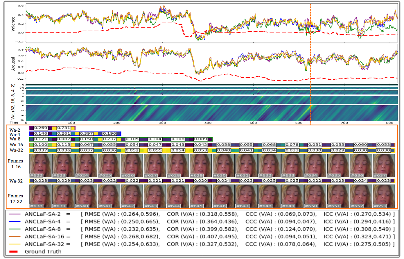
Figure 4: Analysis of the relationship between the selection of sequence length (n) and the learnt weights of our attentional approach. Top: overview of the prediction results of all variants of our models with attention mechanism (ANCLaF-SA-n) alongside their learnt weights. Middle: details for frames 622 to 653 with their associated weights for each model. Bottom: legend containing the quantitative comparisons.

4.4 Analysis of the Role of the Learnt Attentions Weights

To analyse the impact of the attention mechanism on our sequence modelling, we first show in Figure 3 a comparison of our baseline sequence modelling (ANCLaF-S) against ANCLaF-SA with attention activated. In the top part, we can see the predictions from the best performing models with and without attention (ANCLaF-S-8 and ANCLaF-SA-8). Comparing the predictions from both models, we find that the results are quite similar, though in some cases ANCLaF-SA seems to be more accurate and closer to the ground truth. The quantitative accuracy results indicated on the respective legends confirm this observation.

The attention weights learnt by ANCLaF-SA, involving the previous eight frames, are also displayed at the bottom of the prediction plots. We can see that the weights calculated with respect to the associated frames seem to be higher in the presence of changes. Indeed, we observe that the attention weights are usually activated prior to subsequent facial movements. Interestingly, the intensity of the activations also appears to highlight the level of these facial movements, or the changes between frames. For instance, from frames 280-287, we can see that the different level of the weight intensity seems to be small, which also correlates to the subtle changes observed in those frames (e. g., closing of the eyes). In contrast, in frames 643-650, we see high levels of activation on the first few frames that correspond to the more discernible facial movements on the respective frames, such as the changes observed in the mouth area. These correlations illustrate how our models are capable of learning temporal changes.

Figure 4 provides further details on the attention mechanism for different temporal modelling lengths. We can see that all the displayed models show quite smooth results, thanks to the temporal modelling, but not all of them achieve the same accuracy on the predictions. The bottom part of the figure, highlighting the input sequence from frames 622 to 653, can help to provide an intuition about the optimal temporal modelling length, which was found to be about $8$ frames. To this end, let us start by looking at the whole set of 32 frames: we can see that such a sequence of frames comprises multiple facial changes, and considering all of them together makes the training task harder to optimise. On the other hand, if we consider groups of very few frames (e. g., 2 or 4 frames), the system is likely to capture only part of a given facial action, which may impede it to properly interpret it. Therefore, we see that the optimal sequence length is the one that contains enough frames to interpret facial changes without extending too much the temporal context, which may unnecessarily increase training complexity and reduce accuracy.

Finally, it is important to emphasise that the optimal sequence length needs to take into account the frame rate and the specific facial movements that are present in each dataset. In the considered dataset, with an overall frame rates of 50 fps, this length corresponds to 160 ms.

5 CONCLUSIONS

In this work, we have successfully built a sequence-attention based neural network for affect estimations in the wild. We did so by incorporating three major sub-networks: the Generator, which is responsible to extract latent features on each frame; the Discriminator, which is used to supply the first step of affect estimates of emotional quadrant, and the Combiner, which merges latent features and quadrant information to produce the final refined affect estimates of Valence and Arousal on a frame by frame basis. We then added an LSTM layer to allow temporal modelling, which we further enhanced by using step-wise attention modelling. We trained these three major sub-networks in an adversarial setting, and used curriculum learning on the sequential training stages.

We showed the effectiveness of our approach by reporting top state of the art results on two of the most widely used video datasets for affect analysis, namely AFEW-VA and SEWA. Specifically, our baseline models, which operate without any sequence modelling, yield quite competitive results with other models reported in the literature. On the other hand, our more advanced models, which are sequence-based, clearly helped to improve the affect estimates both in qualitative and quantitative terms. Qualitatively, the temporal modelling helped to produce more stable results, with visibly smoother transitions between affect predictions. Quantitatively, our models produced the overall best accuracy results reported so far on both tested datasets.

Within sequence-based models, we observed the highest accuracy improvements when the attention mechanism was included. Detailed analysis of the attention weights highlighted their correlation with the appearance of facial movements, both in terms of (temporal) localisation and intensity. Finally, we found a sequence length of around 160 ms to be the optimum one for temporal modelling, which is consistent with other relevant findings utilising similar lengths.

Future work will need to explore further optimisation of the considered adversarial topologies and attention mechanisms as well as their transferability across databases, cultures, and domains.

REFERENCES

- Aspandi et al., 2020 Aspandi, D., Mallol-Ragolta, A., Schuller, B., and Binefa, X. (2020). Latent-based adversarial neural networks for facial affect estimations. In 2020 15th IEEE FG, pages 348–352, Los Alamitos, CA, USA. IEEE Computer Society.
- Aspandi et al., 2019a Aspandi, D., Martinez, O., and Binefa, X. (2019a). Heatmap-guided balanced deep convolution networks for family classification in the wild. In 2019 14th IEEE FG 2019, pages 1–5.
- Aspandi et al., 2019b Aspandi, D., Martinez, O., Sukno, F., and Binefa, X. (2019b). Fully end-to-end composite recurrent convolution network for deformable facial tracking in the wild. In 2019 14th IEEE FG, pages 1–8.
- Aspandi et al., 2019c Aspandi, D., Martinez, O., Sukno, F., and Binefa, X. (2019c). Robust facial alignment with internal denoising auto-encoder. In 2019 16th Conference on Computer and Robot Vision (CRV), pages 143–150.
- Barros et al., 2018 Barros, P., Churamani, N., Lakomkin, E., Siqueira, H., Sutherland, A., and Wermter, S. (2018). The omg-emotion behavior dataset. In 2018 International Joint Conference on Neural Networks (IJCNN), pages 1–7. IEEE.
- Bengio et al., 2009 Bengio, Y., Louradour, J., Collobert, R., and Weston, J. (2009). Curriculum learning. In Proceedings of the 26th Annual International Conference on Machine Learning, ICML ’09, page 41–48, New York, NY, USA. Association for Computing Machinery.
- Christodoulidis et al., 2016 Christodoulidis, S., Anthimopoulos, M., Ebner, L., Christe, A., and Mougiakakou, S. (2016). Multisource transfer learning with convolutional neural networks for lung pattern analysis. IEEE journal of biomedical and health informatics, 21(1):76–84.
- Comas et al., 2020 Comas, J., Aspandi, D., and Binefa, X. (2020). End-to-end facial and physiological model for affective computing and applications. In 2020 15th IEEE International Conference on Automatic Face and Gesture Recognition (FG 2020) (FG), pages 1–8, Los Alamitos, CA, USA. IEEE Computer Society.
- Cootes et al., 1998 Cootes, T. F., Edwards, G. J., and Taylor, C. J. (1998). Active appearance models. In Burkhardt, H. and Neumann, B., editors, Computer Vision — ECCV’98, pages 484–498, Berlin, Heidelberg. Springer Berlin Heidelberg.
- Dai et al., 2017 Dai, B., Fidler, S., Urtasun, R., and Lin, D. (2017). Towards diverse and natural image descriptions via a conditional gan. In The IEEE International Conference on Computer Vision (ICCV).
- Duo and Song, 2010 Duo, S. and Song, L. (2010). An e-learning system based on affective computing. Physics Procedia, 24.
- Farhadi and Fox, 2018 Farhadi, D. G. A. and Fox, D. (2018). Re 3: Real-time recurrent regression networks for visual tracking of generic objects. IEEE Robot. Autom. Lett., 3(2):788–795.
- Handrich et al., 2020 Handrich, S., Dinges, L., Al-Hamadi, A., Werner, P., and Al Aghbari, Z. (2020). Simultaneous prediction of valence/arousal and emotions on affectnet, aff-wild and afew-va. Procedia Computer Science, 170:634–641.
- Hochreiter and Schmidhuber, 1997 Hochreiter, S. and Schmidhuber, J. (1997). Long short-term memory. Neural Comput., 9(8):1735–1780.
- Huang et al., 2018 Huang, R., Pedoeem, J., and Chen, C. (2018). Yolo-lite: a real-time object detection algorithm optimized for non-gpu computers. In 2018 IEEE International Conference on Big Data (Big Data), pages 2503–2510. IEEE.
- Kim et al., 2018 Kim, C., Li, F., and Rehg, J. M. (2018). Multi-object tracking with neural gating using bilinear lstm. In The European Conference on Computer Vision (ECCV).
- Kollias et al., 2020 Kollias, D., Schulc, A., Hajiyev, E., and Zafeiriou, S. (2020). Analysing affective behavior in the first abaw 2020 competition. arXiv preprint arXiv:2001.11409.
- Kollias et al., 2019 Kollias, D., Tzirakis, P., Nicolaou, M. A., Papaioannou, A., Zhao, G., Schuller, B., Kotsia, I., and Zafeiriou, S. (2019). Deep affect prediction in-the-wild: Aff-wild database and challenge, deep architectures, and beyond. International Journal of Computer Vision, 127(6-7):907–929.
- Kollias and Zafeiriou, 2019 Kollias, D. and Zafeiriou, S. (2019). Expression, affect, action unit recognition: Aff-wild2, multi-task learning and arcface. arXiv preprint arXiv:1910.04855.
- Kossaifi et al., 2017 Kossaifi, J., Tzimiropoulos, G., Todorovic, S., and Pantic, M. (2017). Afew-va database for valence and arousal estimation in-the-wild. Image and Vision Computing, 65:23–36.
- Kossaifi et al., 2019 Kossaifi, J., Walecki, R., Panagakis, Y., Shen, J., Schmitt, M., Ringeval, F., Han, J., Pandit, V., Schuller, B., Star, K., et al. (2019). Sewa db: A rich database for audio-visual emotion and sentiment research in the wild. arXiv preprint arXiv:1901.02839.
- Li et al., 2020 Li, C., Bao, Z., Li, L., and Zhao, Z. (2020). Exploring temporal representations by leveraging attention-based bidirectional lstm-rnns for multi-modal emotion recognition. Information Processing & Management, 57(3):102185.
- Liu et al., 2008 Liu, C., Conn, K., Sarkar, N., and Stone, W. (2008). Online affect detection and robot behavior adaptation for intervention of children with autism. IEEE T Robot, 24:883 – 896.
- Luong et al., 2015 Luong, M.-T., Pham, H., and Manning, C. D. (2015). Effective approaches to attention-based neural machine translation. arXiv preprint arXiv:1508.04025.
- Lv et al., 2017 Lv, J.-J., Shao, X., Xing, J., Cheng, C., and Zhou, X. (2017). A deep regression architecture with two-stage re-initialization for high performance facial landmark detection. 2017 IEEE CVPR, pages 3691–3700.
- Ma et al., 2019 Ma, J., Tang, H., Zheng, W.-L., and Lu, B.-L. (2019). Emotion recognition using multimodal residual lstm network. In Proceedings of the 27th ACM International Conference on Multimedia, pages 176–183.
- McKeown et al., 2010 McKeown, G., Valstar, M. F., Cowie, R., and Pantic, M. (2010). The semaine corpus of emotionally coloured character interactions. In 2010 IEEE Int Con Multi, pages 1079–1084. IEEE.
- Mitenkova et al., 2019 Mitenkova, A., Kossaifi, J., Panagakis, Y., and Pantic, M. (2019). Valence and arousal estimation in-the-wild with tensor methods. In 2019 14th IEEE FG 2019, pages 1–7. IEEE.
- Mollahosseini et al., 2015 Mollahosseini, A., Hasani, B., and Mahoor, M. H. (2015). Affectnet: A database for facial expression. Valence, and Arousal Computing in the Wild Department of Electrical and Computer Engineering, University of Denver, Denver, CO, 80210.
- Nicolaou et al., 2011 Nicolaou, M. A., Gunes, H., and Pantic, M. (2011). Continuous prediction of spontaneous affect from multiple cues and modalities in valence-arousal space. IEEE T Affect Comput, 2(2):92–105.
- Povolny et al., 2016 Povolny, F., Matejka, P., Hradis, M., Popková, A., Otrusina, L., Smrz, P., Wood, I., Robin, C., and Lamel, L. (2016). Multimodal emotion recognition for avec 2016 challenge. In Proceedings of the 6th International Workshop on Audio/Visual Emotion Challenge, AVEC ’16, page 75–82, New York, NY, USA. Association for Computing Machinery.
- Ringeval et al., 2013 Ringeval, F., Sonderegger, A., Sauer, J., and Lalanne, D. (2013). Introducing the recola multimodal corpus of remote collaborative and affective interactions. In 2013 10th IEEE FG, pages 1–8.
- Russell, 1980 Russell, J. A. (1980). A circumplex model of affect. Journal of personality and social psychology, 39(6):1161.
- Schmitt et al., 2019 Schmitt, M., Cummins, N., and Schuller, B. (2019). Continuous emotion recognition in speech–do we need recurrence? Training, 34(93):12.
- Tellamekala and Valstar, 2019 Tellamekala, M. K. and Valstar, M. (2019). Temporally coherent visual representations for dimensional affect recognition. In 2019 8th International Conference on Affective Computing and Intelligent Interaction (ACII), pages 1–7. IEEE.
- Triantafyllidou and Tefas, 2016 Triantafyllidou, D. and Tefas, A. (2016). Face detection based on deep convolutional neural networks exploiting incremental facial part learning. In 2016 23rd International Conference on Pattern Recognition (ICPR), pages 3560–3565.
- Xia et al., 2020 Xia, Y., Braun, S., Reddy, C. K. A., Dubey, H., Cutler, R., and Tashev, I. (2020). Weighted speech distortion losses for neural-network-based real-time speech enhancement. In ICASSP 2020 - 2020 IEEE ICASSP, pages 871–875.
- Xiaohua et al., 2019 Xiaohua, W., Muzi, P., Lijuan, P., Min, H., Chunhua, J., and Fuji, R. (2019). Two-level attention with two-stage multi-task learning for facial emotion recognition. Journal of Visual Communication and Image Representation, 62:217–225.
- Xie et al., 2016 Xie, J., Girshick, R. B., and Farhadi, A. (2016). Deep3d: Fully automatic 2d-to-3d video conversion with deep convolutional neural networks. In ECCV 2016, pages 842–857.
- Ye et al., 2018 Ye, H., Li, G. Y., Juang, B.-H. F., and Sivanesan, K. (2018). Channel agnostic end-to-end learning based communication systems with conditional gan. In 2018 IEEE Globecom Workshops (GC Wkshps), pages 1–5. IEEE.
- Zafeiriou et al., 2017 Zafeiriou, S., Kollias, D., Nicolaou, M. A., Papaioannou, A., Zhao, G., and Kotsia, I. (2017). Aff-wild: Valence and arousal ‘in-the-wild’challenge. In IEEE CVPRW, 2017, pages 1980–1987. IEEE.