On the Mathematics of Swarming:
Emergent Behavior in Alignment Dynamics

Abstract.

We overview recent developments in the study of alignment hydrodynamics, driven by a general class of symmetric communication kernels. A main question of interest is to characterize the emergent behavior of such systems, which we quantify in terms of the spectral gap of a weighted Laplacian associated with the alignment operator. Our spectral analysis of energy fluctuation covers both long-range and short-range kernels and does not require thermal equilibrium (no closure for the pressure). In particular, in the prototypical case of metric-based short-range kernels, the spectral gap admits a lower-bound expressed in terms of the discrete Fourier coefficients of the radial kernel, which enables us to quantify an emerging flocking behavior for non-vacuous solutions. These large-time behavior results apply as long as the solutions remain smooth. It is known that global smooth solutions exist in one and two spatial dimensions, subject to sub-critical initial data. We settle the question for arbitrary dimension, obtaining non-trivial initial threshold conditions which guarantee existence of multiD global smooth solutions.

1. Introduction

The starting point of our discussion is the celebrated Cucker-Smale (CS) model [CS2007a, CS2007b] which describes the dynamics of $N$ particles, viewed as agents, with (position, velocity) pairs $({\mathbf{x}}_{i}(t),{\mathbf{v}}_{i}(t)):\mathbb{R}_{+}\mapsto(\Omega,\mathbb{R}^{d})$,

(1.1) $$\left\{\ \ \begin{split}\dot{{\mathbf{x}}}_{i}(t)&={\mathbf{v}}_{i}(t)\\ \dot{{\mathbf{v}}}_{i}(t)&=\frac{\tau}{N}\sum_{j=1}^{N}\phi_{ij}(t)({\mathbf{v}}_{j}(t)-{\mathbf{v}}_{i}(t)),\end{split}\right.$$

and subject to prescribed initial conditions, $({\mathbf{x}}_{i}(0),{\mathbf{v}}_{i}(0))=({\mathbf{x}}_{i0},{\mathbf{v}}_{i0})\in(\Omega,\mathbb{R}^{d})$. The ambient space of positions $\Omega\subset\mathbb{R}^{d}$ will refer to one of two main scenarios — either $\Omega=\mathbb{R}^{d}$ or $\Omega=\mathbb{T}^{d}$. System (1.1) is a canonical model for alignment dynamics in which pairwise interactions steer towards average heading. Alignment originated in pioneering works [Aok1982, Rey1987, VCBCS1995, CS2007a, CS2007b, CKJRF2002], as a key ingredient in self-organization — a unity from within which leads to the emergence of higher-order, large-scales patterns. It is found in ecology — from flocking of birds and schooling of fish to swarming bacteria and insects; in social dynamics of human interactions — from alignment of pedestrians and emerging consensus of opinions to markets and marketing; and in sensor-based networks — from swarming of mobile robots and control of UAVs to macro-molecules and metallic rods.

The dynamics (1.1) governs pairwise interactions, $\phi_{ij}=\phi({\mathbf{x}}_{i},{\mathbf{x}}_{j})$, dictated by a scalar communication kernel $\phi(\cdot,\cdot)$ with amplitude $\tau>0$. We assume that $\phi(\cdot,\cdot)\in L^{\infty}(\Omega\times\Omega)$ is a non-negative symmetric kernel, properly normalized

(1.2) $$\int_{\Omega}\phi({\mathbf{x}},{\mathbf{x}}^{\prime})\,{\sf{d}}{\mathbf{x}}^{\prime}\equiv 1,\qquad\phi({\mathbf{x}},{\mathbf{x}}^{\prime})=\phi({\mathbf{x}}^{\prime},{\mathbf{x}})\geqslant 0.$$

The role for the kernel $\phi$ is context-dependent: its approximate shape is either derived empirically, deduced from higher order principles, learned from the data or postulated based on phenomenological arguments, e.g., [VCBCS1995, CF2003, CKFL2005, Bal2008, Ka2011, VZ2012, Bia2012, Bia2014, CS2007a, BDT2017, MLK2019, BDT2019, LZTM2019, ST2021] and the references therein. The specific structure of $\phi$, however, is not necessarily known. Instead, we ask how different classes of communication kernels affect the emergent behavior of (1.1). Here are few examples for different communication protocols.
A major part of current literature is devoted to the generic class of metric-based kernels, $\phi({\mathbf{x}},{\mathbf{x}}^{\prime})=\varphi(|{\mathbf{x}}-{\mathbf{x}}^{\prime}|)$. A prototype example which goes back to Cucker-Smale [CS2007a] $\varphi(r)=\langle r\rangle^{-\theta},\ \theta>0$. This is motivated by the phenomenological reasoning that the strength of pairwise interactions is inversely dependent on their relative distance, “birds of feather flock together”. Thus, the emphasize is on the behavior of $\varphi(r)$ for $r\gg 1$. This can be contrasted with an opposite protocol based on tendency to attract diverse groups so that $\varphi(r)$ is increasing over its compact support, e.g., the heterophilous dynamics studied in [MT2014].
An important protocol of metric-based communication which will not be analyzed here includes the class of singular kernels, e.g., the Riesz kernel,

(1.3) $$\varphi(r)=\frac{1}{r^{\beta}},\qquad 0<\beta<d+2,$$

where the communication emphasizes near-by neighbors, $r\ll 1$, over those farther away, e.g., [Pes2015, CCMP2017, ST2017a, ST2018a, DKRT2018, PS2019, MMPZ2019] and the references therein.
Another example is the class of topologically-based kernels, [Bal2008, ST2020b], where $\phi({\mathbf{x}},{\mathbf{x}}^{\prime})=\varphi(\mu({\mathbf{x}},{\mathbf{x}}^{\prime}))$ is dictated by the size of the crowd in an intermediate domain of communication ${\mathcal{C}}({\mathbf{x}},{\mathbf{x}}^{\prime})$ enclosed between ${\mathbf{x}}$ and ${\mathbf{x}}^{\prime}$,

(1.4) $$\mu({\mathbf{x}},{\mathbf{x}}^{\prime}):=\frac{1}{N}\#\{k:\,{\mathbf{x}}_{k}\in{\mathcal{C}}({\mathbf{x}},{\mathbf{x}}^{\prime})\}.$$

In particular, if the domain of communication ${\mathcal{C}}$ is shifted to an $R$-ball centered at ${\mathbf{x}}$, one ends up with the non-symmetric topological kernel [MT2011] $\displaystyle\phi({\mathbf{x}},{\mathbf{x}}^{\prime})={\varphi(|{\mathbf{x}}-{\mathbf{x}}^{\prime}|)}/{\mu(B_{R}({\mathbf{x}}))}$. Other important protocols of communication which will not be analyzed here are based on various random-based protocols found in chemo- and photo-tactic dynamics, the Elo rating system, voter and related opinion-based models, a random-batch method and consensus-based optimization, to name but a few, [DAWF2002, BeN2005, CFL2009, GWBL2012, JJ2015, PTTM2017, CCTT2018, JLL2020].
As a prototype example for ‘higher order principles’ we mention the anticipation-based dynamics [MCEB2015, GTLW2017, ST2021]

$$\dot{{\mathbf{v}}}_{i}(t)=-\frac{1}{N}\sum_{j=1}^{N}\nabla_{i}U(|{\mathbf{x}}_{i}^{\tau}-{\mathbf{x}}_{j}^{\tau}|),$$

in which agents at time $t$ react to the anticipated positions, ${\mathbf{x}}_{j}^{\tau}(t):={\mathbf{x}}_{j}(t)+\tau{\mathbf{v}}_{i}(t)$ at time $t+\tau$. The dynamics is governed by a radial potential $U$. Expanding in the (assumed small) $\tau>0$ we find

(1.5) $$\dot{{\mathbf{v}}}_{i}=\frac{\tau}{N}\sum_{j=1}^{N}\Phi_{ij}({\mathbf{v}}_{j}-{\mathbf{v}}_{i})-\frac{1}{N}\sum_{j=1}^{N}\nabla U(|{\mathbf{x}}_{j}-{\mathbf{x}}_{i}|).$$

The first sum on the right represent the alignment term with amplitude $\tau$, driven by the average Hessian, $\Phi_{ij}=\widetilde{D^{2}U}(|{\mathbf{x}}_{i}-{\mathbf{x}}_{j}|)$, and is a prototype for a a still larger class of symmetric matrix communication kernels; the scalar case $\Phi_{ij}=\phi_{ij}{\mathbb{I}}$ recovers the Cucker-Smale model (1.1). In addition to alignment, there is the second sum on the right of (1.5) which governs pairwise repulsions and attractions, corresponding to $U^{\prime}(|{\mathbf{x}}_{i}-{\mathbf{x}}_{j}|)<0$ and respectively, $U^{\prime}(|{\mathbf{x}}_{i}-{\mathbf{x}}_{j}|)>0$.
A general protocol for rules of engagement, with pairwise interactions driven by alignment, repulsion and attraction which are dominant in three different zones of proximity, was proposed in the pioneering work [Rey1987]. We shall focus here on the emergent behavior of alignment dynamics, and refer to [CFTV2010, CDMBC2007, ST2021] and the references therein, for results related to more general protocols. To date, we still lack a mathematical theory which analyzes the emergent behavior of the general class of 3Zone models for collective dynamics.

1.1. Connectivity

The large time behavior of (1.1) depends on the time-dependent weighted graph with agents at the $N$ vertices ${{\sf V}}(t)=\{i\,|\,{\mathbf{x}}_{i}(t)\}$ and time-dependent edges ${{\sf E}}(t)=\{(i,j)\,|\,i\neq j:\,\phi_{ij}(t)>0\}$. The energy fluctuations associated with (1.1),

$$\delta{\mathscr{E}}(t):=\frac{1}{N^{2}}\sum_{i,j=1}^{N}|{\mathbf{v}}_{i}(t)-{\mathbf{v}}_{j}(t)|^{2},$$

satisfy

(1.6) $$\begin{split}\frac{{\sf{d}}}{{\sf{d}}t}\delta{\mathscr{E}}(t)&=-\frac{2\tau}{N^{2}}\sum_{(i,j)\in{{\sf E}}(t)}\!\!\!\phi_{ij}(t)|{\mathbf{v}}_{i}(t)-{\mathbf{v}}_{j}(t)|^{2}\leqslant-\lambda_{2}(t)\frac{2\tau}{N^{2}}\sum_{i,j=1}^{N}|{\mathbf{v}}_{i}(t)-{\mathbf{v}}_{j}(t)|^{2}.\end{split}$$

The first equality follows directly from (1.1) and the assumed symmetry of the adjacency matrix $\Phi(t)=\{\phi_{ij}(t)\}$. The second inequality is a sharp bound in terms of the spectral gap, $\lambda_{2}(t):=\lambda_{2}(\Delta_{\Phi(t)})$, of the graph Laplacian associated with $\Phi(t)$. Here the graph Laplacian, $(\Delta_{\Phi})_{\alpha\beta}:=(\sum_{\gamma\neq\alpha}\phi_{\alpha\gamma})\delta_{\alpha\beta}-\phi_{\alpha\beta}(1-\delta_{\alpha\beta})$, and its spectral gap coincides with the Fiedler number, [Fie1973, Fie1989],which encodes the connectivity properties of the weighted graph of agents $({{\sf V}}(t),{{\sf E}}(t))$, e.g., [CS2007a]. Indeed, (1.6) tells us that energy fluctuations are depleted as long as the graph remains (algebraically) connected

(1.7) $$\delta{\mathscr{E}}(t)\leqslant exp\left\{-2\tau\!\int^{t}\!\!\lambda_{2}(s){{\sf{d}}}s\right\}\delta{\mathscr{E}}(0).$$

Connectivity — and hence the large time emergence of flocks or swarms, is guaranteed with long-range kernels. In many realistic configurations, however, the communication among ‘social particles’ takes place in local neighborhoods induced by short-range kernels.
Long and short-range communication kernels will be the topic of the next two sections. Long-range kernels maintain connectivity which in turn imply decay of fluctuations around an emergent cluster. The large time dynamics with short-range kernels is considerably more complicated — in particular, algebraically connected initial configurations, $\lambda_{2}(t=0)>0$, may break down into two or more disconnected clusters at a finite time so that $\lambda_{2}(t_{c})=0$. That is, the dynamics with short-range kernels may or may not be stable, which makes it difficult to trace its flocking behavior. Instead, we study here the flocking/swarming behavior with large crowds: large crowd dynamics tends to stabilize the large-time behavior. As already noted by Immanuel Kant in 1784 [Kant1784, p. 11] “what seems complex and chaotic in the single individual may be seen from the standpoint of the human race as a whole to be a steady and progressive though slow evolution of its original endowment”.

1.2. Hydrodynamic description

The large crowd dynamics of (1.1) is encoded in terms of the empirical distribution $f_{N}(t,{\mathbf{x}},{\mathbf{v}})=\frac{1}{N}\sum_{i=1}^{N}\delta_{{\mathbf{x}}_{i}(t)}({\mathbf{x}})\otimes\delta_{{\mathbf{v}}_{i}(t)}({\mathbf{v}})$, which is governed by the kinetic equation in state variables $(t,{\mathbf{x}},{\mathbf{v}})\in\mathbb{R}_{+}\times\Omega\times\mathbb{R}^{d}$, e.g., [HT2008, HL2009, CFTV2010],

(1.8) $$\begin{split}\partial_{t}f_{N}+{\mathbf{v}}\cdot\nabla_{\mathbf{x}}f_{N}=-\tau\nabla_{\mathbf{v}}\cdot Q_{\phi}(f_{N},f_{N}),\qquad(t,{\mathbf{x}},{\mathbf{v}})\in\mathbb{R}_{+}\times\Omega\times\mathbb{R}^{d}.\end{split}$$

It is driven according to the pairwise communication protocol on the right of (1.1)₂

(1.9) $$Q_{\phi}(f,f):=\iint_{\mathbb{R}^{d}\times\Omega}\phi({\mathbf{x}},{\mathbf{x}}^{\prime})({\mathbf{v}}^{\prime}-{\mathbf{v}})f(t,{\mathbf{x}},{\mathbf{v}})f(t,{\mathbf{x}}^{\prime},{\mathbf{v}}^{\prime})\,{\sf{d}}{\mathbf{v}}^{\prime}\,{\sf{d}}{\mathbf{x}}^{\prime}.$$

For $N\gg 1$, the dynamics of $f_{N}(t,{\mathbf{x}},{\mathbf{v}})$ is captured by its first two moments which we assume to exist — the density $\displaystyle\rho(t,{\mathbf{x}}):=\lim_{N\rightarrow\infty}\int_{\mathbb{R}^{d}}f_{N}(t,{\mathbf{x}},{\mathbf{v}})\,\mathrm{d}{\mathbf{v}}$, and the momentum, $\displaystyle\rho{\mathbf{u}}(t,{\mathbf{x}}):=\lim_{N\rightarrow\infty}\int_{\mathbb{R}^{d}}{\mathbf{v}}f_{N}(t,{\mathbf{x}},{\mathbf{v}})\,\mathrm{d}{\mathbf{v}}$. They admit the hydrodynamic description in state variable $(t,{\mathbf{x}})\in(\mathbb{R}_{+}\times\Omega)$,

(1.10a) $$\left\{\ \ \begin{split}\rho_{t}+\nabla_{\mathbf{x}}\cdot(\rho{\mathbf{u}})&=0,\\ (\rho{\mathbf{u}})_{t}+\nabla_{\mathbf{x}}\cdot(\rho{\mathbf{u}}\otimes{\mathbf{u}}+{\mathbb{P}})&=\tau{\mathbf{A}}_{\phi}(\rho,{\mathbf{u}}),\end{split}\right.\qquad(t,{\mathbf{x}})\in\mathbb{R}_{+}\times\Omega.$$

Here, the pressure $${\mathbb{P}}$$ on the left of (1.10a)₂ is a symmetric positive-definite stress tensor

(1.10b) $${\mathbb{P}}(t,{\mathbf{x}}):=\lim_{N\rightarrow\infty}\int_{\mathbb{R}^{d}}({\mathbf{v}}-{\mathbf{u}})({\mathbf{v}}-{\mathbf{u}})^{\top}f_{N}(t,{\mathbf{x}},{\mathbf{v}})\,\mathrm{d}{\mathbf{v}},$$

and $${\mathbf{A}}_{\phi} \phi$$ on the right of (1.10a)₂ is the communication protocol associated with , corresponding to (1.9),

(1.10c) $${\mathbf{A}}_{\phi}(\rho,{\mathbf{u}})(t,{\mathbf{x}}):=\int_{\Omega}\phi({\mathbf{x}},{\mathbf{x}}^{\prime})\big{(}{\mathbf{u}}(t,{\mathbf{x}}^{\prime})-{\mathbf{u}}(t,{\mathbf{x}})\big{)}\rho(t,{\mathbf{x}})\rho(t,{\mathbf{x}}^{\prime})\,{\sf{d}}{\mathbf{x}}^{\prime}.$$

Observe that system (1.10) is not a purely hydrodynamic description at the macroscopic scale: while the density and velocity, $\rho=\rho(t,{\mathbf{x}})$ and ${\mathbf{u}}={\mathbf{u}}(t,{\mathbf{x}})$, are governed by the macroscopic balances (1.10a),(1.10c), the pressure ${\mathbb{P}}$ in (1.10b), ${\mathbb{P}}={\mathbb{P}}(t,{\mathbf{x}})$, still requires a closure of the ${\mathbf{v}}$-dependent second-order moments of $f_{N}$. We recall that in the case of physical particles, one encounters the canonical closure imposed by Maxwellian equilibrium and expressed in terms of the density $\rho$, velocity ${\mathbf{u}}$ and temperature $T$, [Cer1990, Lev1996, Gol1997/98],

$$M_{\{\rho,{\mathbf{u}},T\}}(t,{\mathbf{x}},{\mathbf{v}})=\frac{\rho}{(2\pi T)^{d/2}}\textnormal{exp}\left(-\frac{|{\mathbf{v}}-{\mathbf{u}}|^{2}}{2T}\right).$$

We mention in this context the special cases of mono-kinetic closure, ${\mathbb{P}}\equiv 0$, associated with the vanishing temperature $M_{\{\rho,{\mathbf{u}},T\downarrow 0\}}(t,{\mathbf{x}})=\rho\delta(|{\mathbf{v}}-{\mathbf{u}}|)$, [KV2015, FK2019], an entropic-based closure with measured data in [Bia2012] and the isothermal closure studied in [KMT2015] ${\mathbb{P}}=\rho{\mathbb{I}}_{d\times d}$ (corresponding to constant temperature $T$).
The general case of ‘social particles’, however, is different: there is no universal Maxwellian closure. This issue will be revisited in section 4.1. The question of closure in the context of our discussion on hydrodynamic description for alignment (1.10), is therefore left open. Indeed, we highlight the fact that the decay of energy fluctuations quantified in the next section applies to general mesoscopic pressure stress tensors (1.10b).

1.3. Fluctuations

The total energy of the large-crowd dynamics associated with (1.1) is given by the second moment (which is assumed to exist)

$$\rho E(t,{\mathbf{x}}):=\lim_{N\rightarrow\infty}\int_{\mathbb{R}^{d}}\frac{1}{2}|{\mathbf{v}}|^{2}f_{N}(t,{\mathbf{x}},{\mathbf{v}})\,\mathrm{d}{\mathbf{v}}.$$

It satisfies the energy equation

(1.11) $$(\rho E)_{t}+\nabla_{\mathbf{x}}\cdot(\rho E{\mathbf{u}}+{\mathbb{P}}{\mathbf{u}}+{\mathbf{q}})=-\tau\int\phi({\mathbf{x}},{\mathbf{x}}^{\prime})\big{(}2E(t,{\mathbf{x}})-{\mathbf{u}}\cdot{\mathbf{u}}^{\prime}\big{)}\rho\rho^{\prime}\,{\sf{d}}{\mathbf{x}}^{\prime}.$$

The energy flux on the left of (1.11) is computed as the second moment of (1.8),

$$\lim_{N\rightarrow\infty}\int\frac{|{\mathbf{v}}|^{2}}{2} {\mathbf{v}}f_{N}(t,{\mathbf{x}},{\mathbf{v}})\,\mathrm{d}{\mathbf{v}}={\mathbf{u}}\lim_{N\rightarrow\infty}\int_{\mathbb{R}^{d}}\frac{|{\mathbf{v}}|^{2}}{2}f_{N}\,\mathrm{d}{\mathbf{v}}+\lim_{N\rightarrow\infty}\int_{\mathbb{R}^{d}}\frac{|{\mathbf{v}}|^{2}}{2}({\mathbf{v}}-{\mathbf{u}})f_{N}\,\mathrm{d}{\mathbf{v}}$$

$$=\rho E{\mathbf{u}}+\lim_{N\rightarrow\infty}\int_{\mathbb{R}^{d}}\Big{(}\frac{|{\mathbf{u}}|^{2}}{2}+({\mathbf{v}}-{\mathbf{u}})\cdot{\mathbf{u}}+\frac{|{\mathbf{v}}-{\mathbf{u}}|^{2}}{2}\Big{)}({\mathbf{v}}-{\mathbf{u}})f_{N}\,\mathrm{d}{\mathbf{v}}$$

$$=\rho E{\mathbf{u}}+{\mathbb{P}}{\mathbf{u}}+{\mathbf{q}},$$

expressed in terms of ${\mathbb{P}}$ and the heat flux $\displaystyle{\mathbf{q}}(t,{\mathbf{x}}):=\lim_{N\rightarrow\infty}\frac{1}{2}\int({\mathbf{v}}-{\mathbf{u}})|{\mathbf{v}}-{\mathbf{u}}|^{2}f_{N}(t,{\mathbf{x}},{\mathbf{v}})\,\mathrm{d}{\mathbf{v}}$. The energy production on the right of (1.11) is driven by the enstrophy

$$\iiint\phi({\mathbf{x}},{\mathbf{x}}^{\prime}){\mathbf{v}}\cdot({\mathbf{v}}-{\mathbf{v}}^{\prime})ff^{\prime}\,{\sf{d}}{\mathbf{v}}^{\prime}\,\mathrm{d}{\mathbf{v}}\,{\sf{d}}{\mathbf{x}}^{\prime}=\int\phi({\mathbf{x}},{\mathbf{x}}^{\prime})\big{(}2E({\mathbf{x}})-{\mathbf{u}}\cdot{\mathbf{u}}^{\prime}\big{)}\rho(t,{\mathbf{x}})\rho(t,{\mathbf{x}}^{\prime})\,{\sf{d}}{\mathbf{x}}^{\prime}.$$

The energy can be decomposed as the sum of kinetic and internal energies, $\rho E=\rho e_{K}+\rho e$, corresponding to the first two terms in the decomposition of kinetic velocity $\frac{1}{2}|{\mathbf{v}}|^{2}\equiv\frac{1}{2}|{\mathbf{u}}|^{2}+\frac{1}{2}|{\mathbf{v}}-{\mathbf{u}}|^{2}+({\mathbf{v}}-{\mathbf{u}})\cdot{\mathbf{u}}$,

$$\begin{split}\rho e_{K}(t,{\mathbf{x}})&:=\frac{1}{2}\rho{|{\mathbf{u}}|^{2}(t,{\mathbf{x}})},\\ (\rho e)(t,{\mathbf{x}})&:=\lim_{N\rightarrow\infty}\frac{1}{2}\int|{\mathbf{v}}-{\mathbf{u}}(t,{\mathbf{x}})|^{2}f_{N}(t,{\mathbf{x}},{\mathbf{v}})\,\mathrm{d}{\mathbf{v}}.\end{split}$$

Let $\delta{\mathscr{E}}(t)$ denote the total energy fluctuations at time $t$,

$$\delta{\mathscr{E}}(t):=\frac{1}{2m_{0}}\iint\Big{(}\frac{1}{2}|{\mathbf{u}}(t,{\mathbf{x}})-{\mathbf{u}}(t,{\mathbf{x}}^{\prime})|^{2}+e(t,{\mathbf{x}})+e(t,{\mathbf{x}}^{\prime})\Big{)}\rho\rho^{\prime}\,{\sf{d}}{\mathbf{x}}\,{\sf{d}}{\mathbf{x}}^{\prime}.$$

The first integrand quantifies fluctuations of macroscopic velocities, ${\mathbf{u}}(t,\cdot)$, while the last two terms quantify microscopic fluctuations, $|{\mathbf{v}}-{\mathbf{u}}(t,\cdot)|^{2}$. Its decay rate is given by

(1.12) $$\frac{{\sf{d}}}{{\sf{d}}t}\delta{\mathscr{E}}(t)=-\tau\iint\phi({\mathbf{x}},{\mathbf{x}}^{\prime})\Big{(}\frac{1}{2}|{\mathbf{u}}(t,{\mathbf{x}})-{\mathbf{u}}(t,{\mathbf{x}}^{\prime})|^{2}+e(t,{\mathbf{x}})+e(t,{\mathbf{x}}^{\prime})\Big{)}\rho\rho^{\prime}\,{\sf{d}}{\mathbf{x}}\,{\sf{d}}{\mathbf{x}}^{\prime}.$$

This follows by integration of the energy equation (1.11): on the left we use $\displaystyle 2m_{0}\int\rho E\,{\sf{d}}{\mathbf{x}}=\iint\left[\frac{1}{2}|{\mathbf{u}}|^{2}+\frac{1}{2}|{\mathbf{u}}^{\prime}|^{2}+e+e^{\prime}\right]\rho\rho^{\prime}\,{\sf{d}}{\mathbf{x}}\,{\sf{d}}{\mathbf{x}}^{\prime}$ and the fact that $\displaystyle\frac{{\sf{d}}}{{\sf{d}}t}\int\rho{\mathbf{u}}(t,{\mathbf{x}})\,{\sf{d}}{\mathbf{x}}\equiv 0$; on the right, we use the symmetric part of the enstrophy

$$2E-{\mathbf{u}}\cdot{\mathbf{u}}^{\prime}\equiv\frac{1}{2}|{\mathbf{u}}-{\mathbf{u}}^{\prime}|^{2}+e+e^{\prime}+\frac{1}{2}\big{(}|{\mathbf{u}}|^{2}-|{\mathbf{u}}^{\prime}|^{2}\big{)}+(e-e^{\prime}).$$

Equation (1.12) quantifies the decay of energy fluctuations on the left in terms of the total enstrophy on the right and is a key ingredient in studying the emergent behavior of (1.10).

1.4. Flocking/Swarming

A main feature of the large-crowd hydrodynamics (1.10) is the emerging behavior of flocking — a large-time behavior characterized by the following two features.

(i) Finite diameter — the continuum crowd supported in $${\mathcal{S}}(t)=\operatorname{supp}\{\rho(\cdot,t)\}$$ forms a ‘flock’ with a finite diameter

(1.13a) $$D(t):=\mathop{\sup}_{{\mathbf{x}},{\mathbf{x}}^{\prime}\in{\mathcal{S}}(t)}|{\mathbf{x}}-{\mathbf{x}}^{\prime}|\leqslant D_{+}<\infty,\qquad{\mathcal{S}}(t):=\operatorname{supp}\{\rho(\cdot,t)\};$$

(ii) Alignment — velocity fluctuations inside the flock vanish for $t\gg 1$,

(1.13b) $$\iint|{\mathbf{u}}(t,{\mathbf{x}})-{\mathbf{u}}(t,{\mathbf{x}}^{\prime})|^{2}\rho\rho^{\prime}\,{\sf{d}}{\mathbf{x}}\,{\sf{d}}{\mathbf{x}}^{\prime}\ \stackrel{{\scriptstyle t\rightarrow\infty}}{{\longrightarrow}}0.$$

Remark that one can combines (1.13b) with global time invariant of the momentum $\displaystyle\overline{\rho{\mathbf{u}}}(t):=\int_{\Omega}\rho{\mathbf{u}}(t,{\mathbf{x}})\,{\sf{d}}{\mathbf{x}}$ and mass $\displaystyle m(t):=\int_{\Omega}\rho(t,{\mathbf{x}})\,{\sf{d}}{\mathbf{x}}$, to deduce the emergent behavior towards the average velocity $\displaystyle\overline{{\mathbf{u}}}_{0}$,

(1.14) $$\delta{\mathscr{E}}(t)=\int\left[\frac{1}{2}|{\mathbf{u}}(t,{\mathbf{x}})-\overline{{\mathbf{u}}}_{0}|^{2}+e(t,{\mathbf{x}})\right]\rho(t,{\mathbf{x}})\,{\sf{d}}{\mathbf{x}}\stackrel{{\scriptstyle t\rightarrow\infty}}{{\longrightarrow}}0,\qquad\overline{{\mathbf{u}}}_{0}:=\frac{(\overline{\rho{\mathbf{u}}})_{0}}{m_{0}}.$$

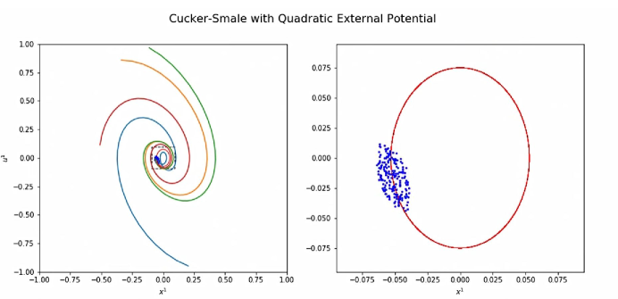
Thus, large time decay of fluctuations takes place while the dynamics is asymptotically aligned along straight particle paths ${\mathbf{x}}_{c}(t)\sim\overline{{\mathbf{u}}}_{0}t$. We mention in passing that the decay of fluctuations in the presence of more general protocol of interactions — repulsion, attraction and external forcing, leads to emergent behavior with different and more ‘interesting’ patterns. For example, when alignment is augmented by pairwise attraction induced by quadratic potential (1.5), it implies flocking of agents which are spatially concentrated along particle path of harmonic oscillators, $({\mathbf{x}}_{c}(t),{\mathbf{u}}_{c}(t)$, depicted in figure 1.1, $\rho{\mathbf{u}}(t,{\mathbf{x}})-m_{0}{\mathbf{u}}_{c}(t)\delta({\mathbf{x}}-{\mathbf{x}}_{c}(t))\stackrel{{\scriptstyle t\rightarrow\infty}}{{\longrightarrow}}0$, [ST2020a, Theorem 2.5]. A rich gallery of emerging swarming patterns is found in [CDMBC2007, CDMBC2007, CDP2009, CFTV2010, BCLR2013].

Figure 1.1. Flocking emerges along harmonic oscillator

Flocking is dictated by the enstrophy on the right of (1.12), which in turn is determined by the two types of fluctuations — the internal energy and kinetic fluctuations. We shall analyze these fluctuations in two separate cases of long-range and short-range communications kernels.

2. Long-range communication kernels

Long range kernels maintain global communication so that each part of the crowd with mass distribution $\rho({\mathbf{x}})\,{\sf{d}}{\mathbf{x}}$ communicates directly with every other part with mass distribution $\rho({\mathbf{x}}^{\prime})\,{\sf{d}}{\mathbf{x}}^{\prime}$. Global communication is quantified in terms of Pareto-type tail

(2.1) $$\phi({\mathbf{x}},{\mathbf{x}}^{\prime})\gtrsim\langle|{\mathbf{x}}-{\mathbf{x}}^{\prime}|\rangle^{-\theta}.$$

According to (1.12), the decay of energy fluctuations requires that the diameter of $\operatorname{supp}\{\rho(\cdot,t)\}$ does not spread too fast.

Corollary 2.1 (Flocking with long-range kernels).

Let $(\rho(t,\cdot),{\mathbf{u}}(t,\cdot),{\mathbb{P}}(t,\cdot))$ be a strong solution of (1.2),(1.10), driven by long-range kernel (2.1). There holds

(2.2) $$\delta{\mathscr{E}}(t)\lesssim exp\,\Big{\{}-\tau\int^{t}\!\!\langle D(s)\rangle^{-\theta}{{\sf{d}}}s\Big{\}}\delta{\mathscr{E}}(0),\qquad D(t):=\operatorname{diam}\operatorname{supp}\{\rho(\cdot,t)\}.$$

The flocking behavior of dynamics driven by long-range kernels is determined by two features: (i) the assumed ‘fat-tail’ behavior (2.1); and (ii) the spread of $\mbox{supp}\{\rho(t,\cdot)\}$. Corollary (2.1) implies that

(2.3) $$\text{if}\ D(t)\lesssim\langle t\rangle^{\beta}\ \text{then flocking follows for}\ \theta\beta<1.$$

‘Fat-tailed’ kernels. A prototype example encountered with uniformly bounded velocity field, in which case $\langle D(t)\rangle\lesssim 2|{\mathbf{u}}|_{\infty}t$ and hence $\beta=1$ implies unconditional flocking for fat-tailed kernels satisfying (2.1) with $\theta\in(0,1)$, which in turn implies fluctuations decay rate of order $\lesssim exp\{-t^{1-\theta}\}$. This is the typical scenario for mono-kinetic closure ${\mathbb{P}}\equiv 0$. In this case, the momentum equation (1.10a)₂ decouples into $d$ scalar transport equations for the components of ${\mathbf{u}}$,

(2.4) $$(\partial_{t}+{\mathbf{u}}\cdot\nabla_{\mathbf{x}})u_{i}=\int\phi({\mathbf{x}},{\mathbf{x}}^{\prime})(u^{\prime}_{i}-u_{i})\rho(t,{\mathbf{x}}^{\prime})\,{\sf{d}}{\mathbf{x}}^{\prime},\qquad{\mathbf{x}}\in\operatorname{supp}\{\rho(\cdot,t)\},$$

each satisfies the maximum principle e.g., [MT2014, Theorem 2.3],[HT2017, $1.1]. In fact, in this pressure-less scenario, (2.4) implies the uniform decay of velocity fluctuations is tied to size of $\operatorname{supp}\{\rho(\cdot,t)\}$

$$\frac{{\sf{d}}}{{\sf{d}}t}V_{i}(t) \leqslant-\tau\langle D(t)\rangle^{-\theta}V_{i}(t),\qquad V_{i}(t)=\max_{{\mathbf{x}},{\mathbf{x}}^{\prime}\in{\mathcal{S}}(t)}|u_{i}(t,{\mathbf{x}})-u_{i}(t,{\mathbf{x}}^{\prime})|$$

$$\frac{{\sf{d}}}{{\sf{d}}t}D(t) \leqslant\max_{i}V_{i}(t).$$

It follows that for the fat-tail alignment (2.1) with $\theta<1$, the following functional [HL2009], $H(t):=\tau\langle D(t)\rangle^{1-\theta}+(1-\theta)\max_{i}V_{i}(t)$, is non-increasing, hence ${\mathcal{S}}(t)$ is, in fact, kept uniformly bounded for all time,

(2.5) $$D(t)\leqslant D_{+},$$

which in turn implies exponential flocking $\lesssim exp\{-\tau D_{+}t\}$. This flocking result for fat-tailed metric-based kernels $\phi({\mathbf{x}},{\mathbf{x}}^{\prime})=\varphi(|{\mathbf{x}}-{\mathbf{x}}^{\prime}|)$, with mono-kinetic closure goes back to Cucker-Smale, e.g., [CS2007a, CS2007b, HT2008, HL2009, CFTV2010, MT2014] and we observe here that it extends to general fat-tailed symmetric kernels.

Another example for flocking occurs with long-range matrix-valued kernels, corresponding to fat-tailed dynamics (2.3) of order $\theta<\nicefrac{{2}}{{3}}$: in this case, the diameter of $\operatorname{supp}\{\rho(\cdot,t)\}$ grows no faster than $D(t)\lesssim\langle t\rangle^{\beta}$ with $\beta<\frac{2}{2-\theta}$, , [ST2021], leading to flocking decay rate of fractional order $\lesssim exp\{-t^{1-\theta\beta}\}$.

Remark 2.2 (Internal energy).

Let $\phi*\rho$ denote the averaged density (recall the normalization (1.2))

(2.6) $$\phi*\rho(t,{\mathbf{x}}):=\int\phi({\mathbf{x}},{\mathbf{x}}^{\prime})\rho(t,{\mathbf{x}}^{\prime})\,{\sf{d}}{\mathbf{x}}^{\prime}\geqslant m_{0}\phi_{-}(t),\qquad\phi_{-}(t)=\min_{{\mathbf{x}},{\mathbf{x}}^{\prime}\in{\mathcal{S}}(t)}\phi({\mathbf{x}},{\mathbf{x}}^{\prime}).$$

We observe that the contribution of the internal energy to the decay of fluctuations in (1.12) admits the lower bound

(2.7) $$\begin{split}\iint\phi({\mathbf{x}},{\mathbf{x}}^{\prime})\big{(}e+e^{\prime}\big{)}\rho\rho^{\prime}\,{\sf{d}}{\mathbf{x}}\,{\sf{d}}{\mathbf{x}}^{\prime}\geqslant\frac{1}{m_{0}}\min_{\mathbf{x}}\phi*\rho(t,{\mathbf{x}})\iint\big{(}e+e^{\prime}\big{)}\rho\rho^{\prime}\,{\sf{d}}{\mathbf{x}}\,{\sf{d}}{\mathbf{x}}^{\prime},\end{split}$$

Hence the decay of the internal energy portion of the fluctuations is independent of the specifics of the closure relationship: any non-negative internal energy is dissipated by fat-tailed kernels, $\phi_{-}(t)\gtrsim\langle D(t)\rangle^{-\theta}$ such that $\displaystyle\int\langle D(s)\rangle^{-\theta}{{\sf{d}}}s=\infty$.

3. Short-range communication kernels

We focus our attention on the more realistic scenario of short-range communication kernels, and in particular, when $\phi({\mathbf{x}},{\mathbf{x}}^{\prime})$ is compactly supported in the vicinity of diagonal $|{\mathbf{x}}-{\mathbf{x}}^{\prime}|<R_{0}$. This means that alignment takes place in local neighborhoods of size $<R_{0}$, which is assumed much smaller than the diameter of the ambient space $\Omega$. We consider the case of $2\pi$-periodic torus $\Omega=\mathbb{T}^{d}$.

3.1. Spectral analysis

We revisit the two ingredients involved in the decay rate of the energy fluctuations stated in (1.12).

(i) Internal energy. We replace the lower bound (2.6) with $\phi*\rho(t,{\mathbf{x}})\geqslant\rho_{-}(t)$ (recall the normalization (1.2)). The decay bound of the internal energy portion in (1.12) for non-vacuous flows then reads

(3.1) $$\iint_{\mathbb{T}^{d}\times\mathbb{T}^{d}}\phi({\mathbf{x}},{\mathbf{x}}^{\prime})\big{(}e+e^{\prime}\big{)}\rho\rho^{\prime}\,{\sf{d}}{\mathbf{x}}\,{\sf{d}}{\mathbf{x}}^{\prime}\geqslant\frac{\rho_{-}(t)}{m_{0}}\iint_{\mathbb{T}^{d}\times\mathbb{T}^{d}}\big{(}e+e^{\prime}\big{)}\rho\rho^{\prime}\,{\sf{d}}{\mathbf{x}}\,{\sf{d}}{\mathbf{x}}^{\prime}.$$

(ii) Kinetic energy. It remains to bound the contribution of the kinetic energy fluctuations to the enstrophy on the right of (1.12)

$$\iint_{\mathbb{T}^{d}\times\mathbb{T}^{d}}\phi({\mathbf{x}},{\mathbf{x}}^{\prime})|{\mathbf{u}}-{\mathbf{u}}^{\prime}|^{2}\rho\rho^{\prime}\,{\sf{d}}{\mathbf{x}}\,{\sf{d}}{\mathbf{x}}^{\prime}.$$

Given the symmetric communication kernel $\phi({\mathbf{x}},{\mathbf{x}}^{\prime})=\phi({\mathbf{x}}^{\prime},{\mathbf{x}})$ we set the weighted Laplacian as the Hilbert-Schmidt operator ${\mathscr{L}}_{\rho}:L^{2}(\mathbb{T}^{d})\rightarrow L^{2}(\mathbb{T}^{d})$,

$$\begin{split}{\mathscr{L}}_{\rho}{\mathbf{w}}({\mathbf{x}}):=\int_{\mathbb{T}^{d}}\phi({\mathbf{x}},{\mathbf{x}}^{\prime})\Big{(}\sqrt{\rho({\mathbf{x}}^{\prime})}{\mathbf{w}}({\mathbf{x}})-\sqrt{\rho({\mathbf{x}})}{\mathbf{w}}({\mathbf{x}}^{\prime})\Big{)}\sqrt{\rho({\mathbf{x}}^{\prime})}\,{\sf{d}}{\mathbf{x}}^{\prime}.\end{split}$$

Let $\lambda_{k}(t)$ be the discrete eigenvalues of ${\mathscr{L}}_{\rho(t)}$ starting with the eigenpair $\lambda_{1}=0$ (corresponding to eigenfunction $\sqrt{\rho(t,{\mathbf{x}})}{\mathbf{c}}$ where ${\mathbf{c}}$ is any constant vector in $\mathbb{R}^{d}$). The desired lower-bound on the kinetic energy fluctuations part of the enstrophy is given by the spectral gap, $\lambda_{2}({\mathscr{L}}_{\rho(t)})$,

(3.2) $$\begin{split}\iint_{\mathbb{T}^{d}\times\mathbb{T}^{d}}\!\!\phi({\mathbf{x}},{\mathbf{x}}^{\prime})&|{\mathbf{u}}-{\mathbf{u}}^{\prime}|^{2}\rho\rho^{\prime}\,{\sf{d}}{\mathbf{x}}\,{\sf{d}}{\mathbf{x}}^{\prime}\geqslant\frac{\lambda_{2}({\mathscr{L}}_{\rho(t)})}{m_{0}}\iint_{\mathbb{T}^{d}\times\mathbb{T}^{d}}\!\!|{\mathbf{u}}-{\mathbf{u}}^{\prime}|^{2}\rho\rho^{\prime}\,{\sf{d}}{\mathbf{x}}\,{\sf{d}}{\mathbf{x}}^{\prime}.\end{split}$$

This corresponds to the bound of energy fluctuations in the discrete case (1.7). The proof is outlined in the end of this section.

Remark 3.1.

The spectral gap bound (3.2) improves the spectral bound derived in [ST2020b, Theorem 1.1] which required the spurious condition $\rho(t,\cdot)\gtrsim\langle t\rangle^{-1/2}$. Instead, (3.2) encodes the behavior of $\rho$ through the weighted Laplacian ${\mathscr{L}}_{\rho(t)}$; its definition is inspired by the discrete weighted Lapalcian introduced in [HT2020, §3].

Inserting (3.1) and (3.2) into (1.12) yields the following.

Theorem 3.2 (Flocking with positive spectral gap).

Let $(\rho(t,\cdot),{\mathbf{u}}(t,\cdot))$ be a strong solution of the hydrodynamic system (1.2),(1.10) with a mesoscopic pressure ${\mathbb{P}}(t,\cdot)$, subject to non-vacuous initial data $(\rho_{0}>0,{\mathbf{u}}_{0},{\mathbb{P}}_{0})$. Then we the following flocking decay estimate holds

(3.3) $$\begin{split}\delta{\mathscr{E}}(t)\leqslant exp\,\Big{\{}-2\tau\int^{t}\min\big{\{}\lambda_{2}({\mathscr{L}}_{\rho(s)}),\rho_{-}(\tau)\big{\}}{{\sf{d}}}s\Big{\}}\delta{\mathscr{E}}(0).\end{split}$$

The energy fluctuations bound (3.3) is in complete analogy with the discrete bound (1.7). In particular, if $\lambda_{2}({\mathscr{L}}_{\rho(t)})$ and $\rho_{-}(t)$ have fat-tailed decay in time, then they ‘communicate’ strong enough alignment to imply the flocking behavior sought in (1.14),

$$\delta{\mathscr{E}}(t)=\int_{\mathbb{T}^{d}}\left[\frac{1}{2}|{\mathbf{u}}(t,{\mathbf{x}})-\overline{{\mathbf{u}}}_{0}|^{2}+e(t,{\mathbf{x}})\right]\rho(t,{\mathbf{x}})\,{\sf{d}}{\mathbf{x}}\rightarrow 0,$$

and it comes with the additional decay of the internal energy.

Proof of the spectral gap bound (3.2).

Given the symmetric communication kernel $\phi({\mathbf{x}},{\mathbf{x}}^{\prime})=\phi({\mathbf{x}}^{\prime},{\mathbf{x}})\in L^{\infty}(\mathbb{T}^{d}\times\mathbb{T}^{d})$ we set the weighted Laplacian operator, ${\mathscr{L}}_{\rho}:=\Lambda_{\rho}-{\mathscr{A}}_{\rho}$ where $\Lambda_{\rho}:L^{2}_{\rho}(\mathbb{T}^{d})\rightarrow L^{2}_{\rho}(\mathbb{T}^{d})$ and ${\mathscr{A}}_{\rho}:L^{2}_{\rho}(\mathbb{T}^{d})\rightarrow L^{2}_{\rho}(\mathbb{T}^{d})$ are a multiplication operator and, respectively, Hilbert-Schmidt operator on $\displaystyle L^{2}_{\rho}(\mathbb{T}^{d}):=\Big{\{}{\mathbf{w}}:\int_{\mathbb{T}^{d}}|{\mathbf{w}}|^{2}\rho\,{\sf{d}}{\mathbf{x}}<\infty\Big{\}}$, which involve the positive weight function $\rho>0$

$$\begin{split}\Lambda_{\rho}{\mathbf{w}}({\mathbf{x}}):=\phi*\rho({\mathbf{x}}){\mathbf{w}}({\mathbf{x}}),\qquad{\mathscr{A}}_{\rho}{\mathbf{w}}({\mathbf{x}}):=\sqrt{\rho({\mathbf{x}})}\int_{\mathbb{T}^{d}}\phi({\mathbf{x}},{\mathbf{x}}^{\prime}){\mathbf{w}}({\mathbf{x}}^{\prime})\sqrt{\rho({\mathbf{x}}^{\prime})}\,{\sf{d}}{\mathbf{x}}^{\prime}.\end{split}$$

The Laplacian ${\mathscr{L}}_{\rho}$ is a symmetric non-negative operator in $L^{2}_{\rho}(\Omega)$:

$$\begin{split}({\mathscr{L}}_{\rho}\sqrt{\rho}{\mathbf{w}},\sqrt{\rho}{\mathbf{w}})&=\iint_{\mathbb{T}^{d}\times\mathbb{T}^{d}}\phi({\mathbf{x}},{\mathbf{x}}^{\prime})\rho({\mathbf{x}}^{\prime})\rho({\mathbf{x}})|{\mathbf{w}}({\mathbf{x}})|^{2}\,{\sf{d}}{\mathbf{x}}\,{\sf{d}}{\mathbf{x}}^{\prime}\\ &\quad-\iint_{\mathbb{T}^{d}\times\mathbb{T}^{d}}\sqrt{\rho({\mathbf{x}})}\phi({\mathbf{x}},{\mathbf{x}}^{\prime})\sqrt{\rho({\mathbf{x}}^{\prime})}\big{\langle}\sqrt{\rho({\mathbf{x}}^{\prime})}{\mathbf{w}}({\mathbf{x}}^{\prime}),\sqrt{\rho({\mathbf{x}})}{\mathbf{w}}({\mathbf{x}})\big{\rangle}\,{\sf{d}}{\mathbf{x}}\,{\sf{d}}{\mathbf{x}}^{\prime}\\ &=\frac{1}{2}\iint_{\mathbb{T}^{d}\times\mathbb{T}^{d}}\phi({\mathbf{x}},{\mathbf{x}}^{\prime})|{\mathbf{w}}({\mathbf{x}})-{\mathbf{w}}({\mathbf{x}}^{\prime})|^{2}\rho({\mathbf{x}})\rho({\mathbf{x}}^{\prime})\,{\sf{d}}{\mathbf{x}}\,{\sf{d}}{\mathbf{x}}^{\prime}.\end{split}$$

Let $(\lambda_{k}\geqslant 0,{\mathbf{w}}_{k}({\mathbf{x}}))$ be the sequence of discrete eigen-pairs of ${\mathscr{L}}_{\rho}$ starting with the eigenpair $(\lambda_{1}=0,{\mathbf{w}}_{1}({\mathbf{x}})=\sqrt{\rho({\mathbf{x}})}{\mathbf{c}})$, where ${\mathbf{c}}$ is any constant vector in $\mathbb{R}^{d}$

$$\begin{split}{\mathscr{L}}_{\rho}{\mathbf{w}}_{1}&=\Lambda_{\rho}(\sqrt{\rho({\mathbf{x}})}{\mathbf{c}})-{\mathscr{A}}_{\rho}(\sqrt{\rho({\mathbf{x}})}{\mathbf{c}})\\ &=\sqrt{\rho({\mathbf{x}})}\int_{\mathbb{T}^{d}}\phi({\mathbf{x}},{\mathbf{x}}^{\prime})\Big{(}\rho({\mathbf{x}}^{\prime})-\sqrt{\rho({\mathbf{x}}^{\prime})}\sqrt{\rho({\mathbf{x}}^{\prime})}\Big{)}\,{\sf{d}}{\mathbf{x}}^{\prime}\times{\mathbf{c}}=0.\end{split}$$

We then have

(3.4) $$\begin{split}\lambda_{2}({\mathscr{L}}_{\rho})&=\inf_{\sqrt{\rho}{\mathbf{w}}\perp\sqrt{\rho}{\mathbf{c}}}\frac{({\mathscr{L}}_{\rho}\sqrt{\rho}{\mathbf{w}},\sqrt{\rho}{\mathbf{w}})}{(\sqrt{\rho}{\mathbf{w}},\sqrt{\rho}{\mathbf{w}})}\\ &=\inf\left\{\frac{\displaystyle\frac{1}{2}\iint\phi({\mathbf{x}},{\mathbf{x}}^{\prime})|{\mathbf{w}}-{\mathbf{w}}^{\prime})|^{2}\rho\rho^{\prime}\,{\sf{d}}{\mathbf{x}}\,{\sf{d}}{\mathbf{x}}^{\prime}}{\displaystyle\frac{1}{2m_{0}}\iint|{\mathbf{w}}-{\mathbf{w}}^{\prime}|^{2}\rho\rho^{\prime}\,{\sf{d}}{\mathbf{x}}\,{\sf{d}}{\mathbf{x}}^{\prime}}\ \ :\ \ \int\rho{\mathbf{w}}=0\right\}.\end{split}$$

The desired lower-bound of the kinetic energy fluctuations (3.2) follows. ∎

3.2. Metric-based communication kernels

The main difficulty with theorem 3.2 is access to the spectral gap $\lambda_{2}({\mathscr{L}}_{\rho(t)})$. To this end, we restrict attention to radial communication kernel, $\phi({\mathbf{x}},{\mathbf{x}}^{\prime})=\varphi(|{\mathbf{x}}-{\mathbf{x}}^{\prime}|)$, over the $2\pi$-periodic torus $\mathbb{T}^{d}$. Short-range communication refers to ’thin tail’ kernels, and in particular — kernels with finite support, (much) smaller than the diameter of the ‘crowd’, $\text{supp}\{\varphi(\cdot)\}<2\pi$, so that there is lack of global direct communication. Instead, decay of energy fluctuations (and hence flocking) persists for non-vacuous configurations quantified below. We denote

$$c_{\rho}(t):=\frac{\rho_{-}(t)}{\rho_{+}(t)},\qquad\rho_{\pm}(t):=\begin{subarray}{c}{\displaystyle\max}_{\mathbf{x}}\\ {\displaystyle\min}_{\mathbf{x}}\end{subarray}\rho(t,{\mathbf{x}}).$$

Theorem 3.3 (Flocking with short-range kernels).

Consider the hydrodynamic system (1.10) over the $2\pi$-periodic torus $\mathbb{T}^{d}$, driven by a non-negative radial communication kernel, $\phi({\mathbf{x}},{\mathbf{x}}^{\prime})=\varphi(|{\mathbf{x}}-{\mathbf{x}}^{\prime}|)$, with unit mass $\displaystyle\int_{{\mathbb{T}}^{d}}\varphi(|{\mathbf{x}}|)\,{\sf{d}}{\mathbf{x}}=1$. Let $(\rho,{\mathbf{u}},{\mathbb{P}})$ be a strong solution subject to non-vacuous initial data $(\rho_{0}>0,{\mathbf{u}}_{0},{\mathbb{P}}_{0})$. There exists a constant

$$\sigma_{\varphi}:=1-\max_{{\bf k}\neq\{\mathbf{0}\}}\int_{{\mathbb{T}}^{d}}\varphi(|{\mathbf{x}}|)\cos\big{(}{\bf k}\cdot{\mathbf{x}}\big{)}\,{\sf{d}}{\mathbf{x}}>0$$

such that

(3.5) $$\lambda_{2}({\mathscr{L}}_{\rho(t)})\geqslant\frac{1}{2}\sigma_{\varphi}c_{\rho}(t)\rho_{-}(t),$$

and the following bound on the decay of energy fluctuations holds

(3.6) $$\delta{\mathscr{E}}(t)\leqslant exp\left\{\displaystyle-\tau\sigma_{\varphi}\!\int^{t}\!\!c_{\rho}(s)\rho_{-}(\tau){{\sf{d}}}s\right\}\delta{\mathscr{E}}(0).$$

Remark 3.4 (Optimality of the spectral gap bound?).

The obvious bound

$$\lambda_{2}(L_{\rho(t)})\geqslant m_{0}\cdot\min\phi({\mathbf{x}},{\mathbf{x}}^{\prime}),$$

implies that when $\phi$ is a long-range communication kernel, namely — when (2.1) holds with $\theta<1$, then it induces an unconditional flocking. The question of flocking for short-range kernels is more subtle: theorem 3.3 shifts the burden of proving flocking in this case to a question of non-vacuous bounded density, $\rho_{-}(t)\gtrsim\langle t\rangle^{-1/2}$. We raise the question whether an improved bound of the spectral gap holds — independent of the aspect ratio $c_{\rho}$, $\lambda_{2}({\mathscr{L}}_{\rho(t)})\gtrsim\rho_{-}(t)$: this would imply flocking for ‘fat-tailed’ density such that $\displaystyle\rho_{-}(t)\gtrsim\langle t\rangle^{-1}$.

Proof of theorem 3.3.

We begin with the following Poincaré inequality, corresponding to the bound of discrete energy fluctuations in (1.6): for all $2\pi$-periodic ${\mathbf{w}}\in L^{2}({\mathbb{T}}^{d})$ there holds

(3.7) $$\iint_{\mathbb{T}^{d}\times\mathbb{T}^{d}}\varphi(|{\mathbf{x}}-{\mathbf{x}}^{\prime}|)|{\mathbf{w}}({\mathbf{x}})-{\mathbf{w}}({\mathbf{x}}^{\prime})|^{2}\,{\sf{d}}{\mathbf{x}}\,{\sf{d}}{\mathbf{x}}^{\prime}\geqslant\frac{\sigma_{\varphi}}{(2\pi)^{d}}\iint_{\mathbb{T}^{d}\times\mathbb{T}^{d}}|{\mathbf{w}}({\mathbf{x}})-{\mathbf{w}}({\mathbf{x}}^{\prime})|^{2}\,{\sf{d}}{\mathbf{x}}\,{\sf{d}}{\mathbf{x}}^{\prime}.$$

Indeed, expressed in terms of the Fourier expansion

$${\mathbf{w}}({\mathbf{x}})=(2\pi)^{-\frac{d}{2}}\sum_{\bf k}\widehat{{\mathbf{w}}}({\bf k})e^{i{\bf k}\cdot{\mathbf{x}}},\qquad\widehat{{\mathbf{w}}}({\bf k})=(2\pi)^{-\frac{d}{2}}\int_{{\mathbb{T}}^{d}}{\mathbf{w}}({\mathbf{x}})e^{-i{\bf k}\cdot{\mathbf{x}}}\,{\sf{d}}{\mathbf{x}},$$

the integral on the right of (3.7) amounts to

(3.8) $$\begin{split}\frac{1}{2}\iint_{\mathbb{T}^{d}\times\mathbb{T}^{d}}|{\mathbf{w}}({\mathbf{x}})-{\mathbf{w}}({\mathbf{x}}^{\prime})|^{2}\,{\sf{d}}{\mathbf{x}}\,{\sf{d}}{\mathbf{x}}^{\prime}&=(2\pi)^{d}\!\int_{{\mathbb{T}}^{d}}|{\mathbf{w}}({\mathbf{x}})|^{2}\,{\sf{d}}{\mathbf{x}}-\Big{|}\int_{{\mathbb{T}}^{d}}{\mathbf{w}}({\mathbf{x}})\,{\sf{d}}{\mathbf{x}}\Big{|}^{2}\\ &=(2\pi)^{d}\sum_{{\bf k}\neq{\mathbf{0}}}|\widehat{{\mathbf{w}}}({\bf k})|^{2}.\end{split}$$

Computing the convolution terms on the left of (3.7), $\widehat{\langle\varphi*{\mathbf{w}}\rangle}({\bf k})=(2\pi)^{\frac{d}{2}}\langle\widehat{\varphi}({\bf k}),\widehat{{\mathbf{w}}}({\bf k})\rangle$, and using the assumed unit mass $\widehat{\varphi}(0)=(2\pi)^{-\frac{d}{2}}$, yields (3.7):

(3.9) $$\begin{split}\frac{1}{2}\iint_{\mathbb{T}^{d}\times\mathbb{T}^{d}}&\varphi(|{\mathbf{x}}-{\mathbf{x}}^{\prime}|)|{\mathbf{w}}-{\mathbf{w}}^{\prime}|^{2}\,{\sf{d}}{\mathbf{x}}\,{\sf{d}}{\mathbf{x}}^{\prime}\\ &=\int_{{\mathbb{T}}^{d}}|{\mathbf{w}}({\mathbf{x}})|^{2}\,{\sf{d}}{\mathbf{x}}-{\mathrm{R}e}\int_{{\mathbb{T}}^{d}}\big{\langle}{\mathbf{w}}({\mathbf{x}}),(\varphi*{\mathbf{w}})({\mathbf{x}})\big{\rangle}\,{\sf{d}}{\mathbf{x}}\\ &=\sum_{{\bf k}\neq{\mathbf{0}}}\left(1-{\mathrm{R}e}\int_{{\mathbb{T}}^{d}}\varphi(|{\mathbf{x}}|)e^{i{\bf k}\cdot{\mathbf{x}}}\,{\sf{d}}{\mathbf{x}}\right)|\widehat{{\mathbf{w}}}({\bf k})|^{2}\\ &\geqslant\left(1-\max_{{\bf k}\neq{\mathbf{0}}}\int_{{\mathbb{T}}^{d}}\varphi({\mathbf{x}})\cos({\bf k}\cdot{\mathbf{x}})\,{\sf{d}}{\mathbf{x}}\right)\sum_{{\bf k}\neq{\mathbf{0}}}|\widehat{{\mathbf{w}}}({\bf k})|^{2}.\end{split}$$

Using (3.7) we compute the lower-bound

$$\begin{split}\iint_{\mathbb{T}^{d}\times\mathbb{T}^{d}}&\varphi(|{\mathbf{x}}-{\mathbf{x}}^{\prime}|)|{\mathbf{u}}-{\mathbf{u}}^{\prime}|^{2}\rho\rho^{\prime}\,{\sf{d}}{\mathbf{x}}\,{\sf{d}}{\mathbf{x}}^{\prime}\\ &\geqslant\rho_{-}^{2}(t)\iint\varphi(|{\mathbf{x}}-{\mathbf{x}}^{\prime}|)|{\mathbf{u}}-{\mathbf{u}}^{\prime}|^{2}\,{\sf{d}}{\mathbf{x}}\,{\sf{d}}{\mathbf{x}}^{\prime}\geqslant\frac{\sigma_{\varphi}}{(2\pi)^{d}}\rho_{-}^{2}(t)\iint|{\mathbf{u}}-{\mathbf{u}}^{\prime}|^{2}\,{\sf{d}}{\mathbf{x}}\,{\sf{d}}{\mathbf{x}}^{\prime}\\ &\geqslant\frac{\sigma_{\varphi}}{(2\pi)^{d}}\frac{\rho_{-}^{2}(t)}{\rho_{+}(t)}(2\pi)^{d}\iint|{\mathbf{u}}-{\mathbf{u}}^{\prime}|^{2}\rho(t,{\mathbf{x}})\,{\sf{d}}{\mathbf{x}}\,{\sf{d}}{\mathbf{x}}^{\prime}\geqslant\sigma_{\varphi}\frac{\rho_{-}^{2}(t)}{\rho_{+}(t)}\frac{1}{m_{0}}\iint|{\mathbf{u}}-\overline{{\mathbf{u}}}_{0}|^{2}\rho\rho^{\prime}\,{\sf{d}}{\mathbf{x}}\,{\sf{d}}{\mathbf{x}}^{\prime}\\ &=\sigma_{\varphi}\frac{\rho_{-}^{2}(t)}{\rho_{+}(t)}\frac{1}{2m_{0}}\iint_{\mathbb{T}^{d}\times\mathbb{T}^{d}}|{\mathbf{u}}-{\mathbf{u}}^{\prime}|^{2}\rho\rho^{\prime}\,{\sf{d}}{\mathbf{x}}\,{\sf{d}}{\mathbf{x}}^{\prime}.\end{split}$$

(Recall $\displaystyle\overline{{\mathbf{u}}}=\frac{\overline{\rho{\mathbf{u}}}}{m_{0}}$ so the fourth inequality follows from $\displaystyle\int|{\mathbf{u}}-{\mathbf{c}}|^{2}\rho\geqslant\int|{\mathbf{u}}-\overline{{\mathbf{u}}}|^{2}\rho$ for all constant vectors ${\mathbf{c}}$). We now deduce (3.5) from the optimaility of $\lambda_{2}({\mathscr{L}}_{\rho})$ in (3.4); observe that the eigenspace associated with $\lambda_{2}({\mathscr{L}}_{\rho(t)})$ remains uniformly bounded away from the eigenspace of constants associated with $\lambda_{1}({\mathscr{L}}_{\rho(t)})=0$. Moreover, $\displaystyle\frac{1}{2}\sigma_{\varphi}c_{\rho}\rho_{-}(t)\leqslant\rho_{-}(t)\leqslant\phi*\rho(t)$ and the (3.6) follows from theorem 3.2. ∎

Let $\overline{m}_{0}$ denote the average mass $\displaystyle\overline{m}_{0}:=\frac{m_{0}}{(2\pi)^{d}}$. Theorem 3.3 implies that as long density fluctuations remains below a specified threshold; there exists a constant $c<1$ such that

(3.10) $$\rho_{+}(t)-\rho_{-}(t)\leqslant(1-c)\overline{m}_{0},\qquad c<1;$$

then $c_{\rho}(t)\geqslant c$ and hence $\displaystyle\rho_{-}(t)\geqslant\overline{m}_{0}c$. We end up with the exponential flocking bound

(3.11) $$\delta{\mathscr{E}}(t)\leqslant e^{-\delta\sigma_{\varphi}t}\delta{\mathscr{E}}(0),\qquad\delta:=\tau\overline{m}_{0}c^{2},\ \ 0<c<1.$$

This echos a similar result for first-order consensus dynamics encoded in terms of $\{{\mathbf{x}}_{i}\}\leadsto\rho$: if the variation of the density remains below a specified $\varphi$-dependent threshold then smooth solutions of approach a consensus, [GPY2017]. In both cases, the threshold, quantified in terms of the Fourier transform of $\varphi$, dictates flocking/consensus for short-range kernels. We close the section with two examples.

3.3. Examples

Example 1. Consider the 1D dynamics over the $2\pi$-torus $\mathbb{T}$ driven by the communication kernel $\phi(x,{x}^{\prime})=\frac{1}{2}\mathds{1}(|x-{x}^{\prime}|)$. The corresponding threshold is given by $\displaystyle\sigma_{\varphi}=1-\sin(1)\sim 0.158$. It follows that if the density has a finite variation so that (3.10) holds, then the 1D CS dynamics (1.10) admits exponentially converging flocking $\lesssim e^{-0.158\delta t}$. In fact, in a recent work of Dietert and Shvydkoy [DS2020, Theorem 1.3] it was shown that in the special 1D case, any discrete CS dynamics (1.1) with non-trivial communication kernel admits flocking rate of order $\lesssim\left(\nicefrac{{\ln(t)}}{{t}}\right)^{1/5}$. Here, by restricting attention to large-crowd dynamics with slowly varying density, we improve the flocking result to exponential rate.

Example 2. Consider the 2D dynamics over the $2\pi$-periodic torus $\mathbb{T}^{2}$ driven by the communication kernel $\phi({\mathbf{x}},{\mathbf{x}}^{\prime})=\frac{1}{\pi}\mathds{1}(|{\mathbf{x}}-{\mathbf{x}}^{\prime}|)$. The Fourier coefficients of the radial $\phi$ are given by, [PST1993], $\displaystyle 2\pi\widehat{\varphi}({\bf k})=\frac{2}{|{\bf k}|}J_{1}(|{\bf k}|)$ and hence

$$\sigma_{\varphi}=1-\frac{J_{1}(1)}{\pi}\sim 0.86.$$

It follows that if the density variation remains with the range (3.10) then the 2D CS dynamics (1.10) admits exponentially converging flocking $\lesssim e^{-0.86\delta t}$.

4. Global smooth solutions: critical thresholds

The hydrodynamics (1.10) is driven by two competing mechanisms: a generic effect in Eulerian dynamics of steepening local fluctuations which may lead to finite-time blow-up when $\displaystyle\lim_{(t,{\mathbf{x}})\uparrow(t_{c},{\mathbf{x}}_{c})}\nabla_{\mathbf{x}}\cdot{\mathbf{u}}(t,{\mathbf{x}})=-\infty$, and alignment which prevents the formation of shock discontinuities,

(4.1) $$\nabla_{\mathbf{x}}\cdot{\mathbf{u}}(t,\cdot)\geqslant-C_{0}>-\infty,$$

as $|{\mathbf{u}}-{\mathbf{u}}^{\prime}|^{2}\rho\rho^{\prime}\,{\sf{d}}{\mathbf{x}}\,{\sf{d}}{\mathbf{x}}^{\prime}\stackrel{{\scriptstyle t\rightarrow\infty}}{{\longrightarrow}}0$. The outcome of this competition determines whether (1.10) admits strong solutions sought in theorems 3.2 and 3.3. The global existence results available in current literature are almost exclusively devoted to mono-kinetic closure ${\mathbb{P}}\equiv 0$,

(4.2) $$\left\{\ \ \begin{split}\rho_{t}+\nabla_{\mathbf{x}}\cdot(\rho{\mathbf{u}})&=0,\\ (\rho{\mathbf{u}})_{t}+\nabla_{\mathbf{x}}\cdot(\rho{\mathbf{u}}\otimes{\mathbf{u}})&=\tau\int_{\mathbb{R}^{d}}\phi({\mathbf{x}},{\mathbf{x}}^{\prime})\big{(}({\mathbf{u}}(t,{\mathbf{x}}^{\prime})-{\mathbf{u}}(t,{\mathbf{x}})\big{)}\rho(t,{\mathbf{x}}^{\prime})\rho(t,{\mathbf{x}})\,{\sf{d}}{\mathbf{x}}^{\prime}.\end{split}\right.$$

This is the default closure relation used in much of the ‘macroscopic’ literature, e.g., [BDT2017, BDT2019] and the references therein.

Although the repulsive forcing of pressure is missing, system (4.2) is still driven by a competition between nonlinear advection and alignment. Indeed, the alignment hydrodynamics with or without pressure, (1.10) or (4.2), may form finite time shock-discontinuities coupled with the emergence of Dirac mass which require their interpretation as weak solutions, e.g., [KMT2013]. A proper notion of weak solutions which enforces uniqueness within an admissible class of solutions is still missing. A theory of dissipative weak solutions was developed in [CFGS2017] in which the authors establish a weak-strong uniqueness principle. Existence of global strong solutions, on the other hand, depend on certain critical thresholds in the space of initial configurations.

4.1. Critical thresholds

To motivate our choice for initial thresholds, we turn to discuss the thermodynamics of the general alignment system (1.10). The entities governed by collective description (1.1) are fundamentally different then physical particles. While physical particles are driven by forces induced by the environment of other particles, the ‘social particles’ we consider here are driven by probing the environment — living organisms, human interactions and sensor-based agents have senses and sensors with which they actively probe the environment. In particular, such social agents receive energy from the outside, thus forming thermo-dynamically open systems. This is particularly apparent in self-organization of biological agents that receive energy from the outside, , thus forming thermo-dynamically open systems, e.g., [Kar2008]. Accordingly, the meso-scopic description for flocking cannot not be expected to provide a self-contained notion of thermodynamic closure sought in (1.10), and as such, there is no universal Maxwellian for thermal equilibrium. As noted in [VZ2012, §1.1], ‘The source of energy making the motion possible … are not relevant’. Nevertheless, lack of thermal equilibrium in the form of certain closure equalities can be substituted with certain inequalities which are compatible with the decay of internal energy fluctuations in (1.12). To this end, we trace the separate contributions of the kinetic and internal energies. Multiply the momentum (1.10a)₂ by ${\mathbf{u}}$, we find

$$\begin{split}\partial_{t}(\rho e_{K})+\nabla_{\mathbf{x}}\cdot\Big{(}\rho{\mathbf{u}}\frac{|{\mathbf{u}}|^{2}}{2}+{\mathbb{P}}{\mathbf{u}}\Big{)}+\sum_{i,j}P_{ij}\frac{\partial u_{i}}{\partial x_{j}}=-\tau\int\phi({\mathbf{x}},{\mathbf{x}}^{\prime})\big{(}|{\mathbf{u}}|^{2}-{\mathbf{u}}\cdot{\mathbf{u}}^{\prime}\big{)}\rho\rho^{\prime}\,{\sf{d}}{\mathbf{x}}^{\prime}.\end{split}$$

Subtract the portion of kinetic energy from the balance of total energy in (1.11) we find the dynamics for the internal energy, expressed in terms of the average density (2.6), $\phi*\rho=\int\phi({\mathbf{x}},{\mathbf{x}}^{\prime})\rho(t,{\mathbf{x}}^{\prime})\,{\sf{d}}{\mathbf{x}}^{\prime}$ and the $d\times d$ velocity gradient matrix $\displaystyle\nabla{\mathbf{u}}:=\Big{\{}\frac{\partial u_{i}}{\partial x_{j}}\Big{\}}$,

$$\begin{split}\partial_{t}(\rho e)+\nabla_{\mathbf{x}}\!\cdot\!({\mathbf{u}}\rho e+{\mathbf{q}})=-\textnormal{trace}\Big{(}{\mathbb{P}}\nabla{\mathbf{u}}\Big{)}-2\tau\rho e\phi*\rho(t,{\mathbf{x}}).\end{split}$$

Since $\displaystyle\textnormal{trace}({\mathbb{P}})=\int|{\mathbf{v}}-{\mathbf{u}}|^{2}f({\mathbf{v}})\,\mathrm{d}{\mathbf{v}}=2\rho e>0$, we can rewrite the equation governing the internal energy

(4.3) $$\begin{split}\partial_{t}(\rho e)+\nabla_{\mathbf{x}}\!\cdot\!({\mathbf{u}}\rho e+{\mathbf{q}})=-2{\mathcal{J}}\rho e\end{split}$$

where ${\mathcal{J}}={\mathcal{J}}(t,{\mathbf{x}})$ is given in terms of the normalized pressure $\displaystyle\overline{{\mathbb{P}}}=\frac{{\mathbb{P}}}{\textnormal{trace}\left({\mathbb{P}}\right)}$

(4.4) $${\mathcal{J}}(t,{\mathbf{x}}):=\textnormal{trace}(\overline{{\mathbb{P}}}\nabla{\mathbf{u}})(t,{\mathbf{x}})+\tau\phi*\rho(t,{\mathbf{x}}),\qquad\overline{{\mathbb{P}}}=\frac{{\mathbb{P}}}{\textnormal{trace}\left({\mathbb{P}}\right)}.$$

We do not enforce any specific form for closure of the internal energy. Instead, we explore the flocking dynamics subject to a rather general set thermodynamic configurations with the minimal assumption, in agreement with (1.12), that the total amount of internal energy is non-increasing. Integration yields

$$\int\rho e(t,{\mathbf{x}})\,{\sf{d}}{\mathbf{x}}\leqslant\textnormal{exp}\left\{-2\int^{t}{\mathcal{J}}_{-}(s)\text{d}s\right\}\int(\rho e)_{0}({\mathbf{x}})\,{\sf{d}}{\mathbf{x}},\qquad{\mathcal{J}}_{-}(t):=\min_{{\mathbf{x}}}\,{\mathcal{J}}(t,{\mathbf{x}}).$$

Thus, a non-increasing total energy is tied to the inequality ${\mathcal{J}}_{-}(t)\geqslant 0$ (and in fact, if there is no heat flux, ${\mathbf{q}}\equiv 0$, then (4.3) would yield a uniform decay of internal energy in thsi case). A simple exercise shows that since $\overline{{\mathbb{P}}}$ is a symmetric positive definite matrix with trace $1$, then $\textnormal{trace}(\overline{{\mathbb{P}}}{\mathbb{M}})\geqslant\lambda_{\textnormal{min}}({\mathbb{M}}_{S})$ for any matrix ${\mathbb{M}}$ with symmetric part ${\mathbb{M}}_{S}:=\frac{1}{2}({\mathbb{M}}+{\mathbb{M}}^{\top})$. In particular we have the following lower-bound in terms of the symmetric gradient $\nabla_{\!\!{}_{S}}{\mathbf{u}}$

(4.5) $$\textnormal{trace}\Big{(}\overline{{\mathbb{P}}}\nabla{\mathbf{u}}\Big{)}\geqslant\lambda_{\textnormal{min}}(\nabla_{\!\!{}_{S}}{\mathbf{u}}),\qquad\nabla_{\!\!{}_{S}}{\mathbf{u}}:=\frac{1}{2}\left(\partial_{j}u_{i}+\partial_{i}u_{j}\right).$$

We therefore postulate the following critical threshold requirement: there exists $\eta_{c}\geqslant 0$ such that

(4.6) $$\eta(\rho,{\mathbf{u}})(t,{\mathbf{x}}):=\lambda_{\textnormal{min}}(\nabla_{\!\!{}_{S}}{\mathbf{u}})(t,{\mathbf{x}})+\tau\phi*\rho(t,{\mathbf{x}})\geqslant\eta_{c},\qquad\eta_{c}\geqslant 0.$$

Observe that the threshold (4.6) is independent of the thermodynamic state of the system and it will guarantee the decay $\displaystyle\int\rho e(t,{\mathbf{x}})\,{\sf{d}}{\mathbf{x}}\lesssim e^{-2\eta_{c}t}$. The key question is whether such threshold persists in time.

At this point it instructive to compare (4.6) with the known results of global regularity in dimension $d=1,2$. A global smooth solution in the 1D case exists if and only if the initial configuration satisfies the threshold $u^{\prime}_{0}(x)+\tau\varphi*\rho_{0}(x)\geqslant 0$, [CCTT2016, TT2014, Les2020] and the extension to uni-directional flows is found in [LS2019]; this corresponds to (4.6)_t=0 with $\eta_{c}=0$. A sufficient threshold for 2D regularity was derived in [HT2017]. It requires a lower bound on the initial divergence and an upper-bound on the spectral gap (recall (2.5))

$$\begin{split}\nabla_{\mathbf{x}}\cdot{\mathbf{u}}_{0}+\tau\varphi*\rho_{0}&>0,\\ (\lambda_{2}-\lambda_{1})(\nabla_{\!\!{}_{S}}{\mathbf{u}}_{0})&\leqslant\delta_{0},\qquad\delta_{0}=:\frac{1}{2}m_{0}\phi(D_{+}),\end{split}$$

which imply that (4.6)_t=0 holds with $\eta_{c}=\frac{1}{2}(\min_{\mathbf{x}}\varphi*\rho_{0}-\delta_{0})$. Existence of strong solutions in $d\geqslant 3$-dimensions for ‘small data’ can be found in [HKK2014, Sh2019]). The next result settles the open question of existence of strong solutions in $d\geqslant 3$ dimensions.

Theorem 4.1 (Existence of global strong solutions for multiD Euler alignment system [Tad2021]).

Consider the Euler alignment system (4.2) subject to non-vacuous initial data, $(\rho_{0},{\mathbf{u}}_{0})\in H^{m}\times H^{m+1}$ with initial velocity of finite variation $\max_{\mathbf{x}}|{\mathbf{u}}^{\prime}_{0}-{\mathbf{u}}_{0}|\leqslant C_{\phi}$. If the initial conditions satisfy the threshold condition

$$\lambda_{\textnormal{min}}(\nabla_{\!\!{}_{S}}{\mathbf{u}}_{0})({\mathbf{x}})+\tau\phi*\rho_{0}({\mathbf{x}})\geqslant\eta_{c},\qquad\eta_{c}=\frac{1}{2}(\rho_{0})_{-}>0,$$

then this threshold persists in time,

$$\lambda_{\textnormal{min}}(\nabla_{\!\!{}_{S}}{\mathbf{u}})(t,{\mathbf{x}})+\tau\phi*\rho(t,{\mathbf{x}})\geqslant\eta_{c},\qquad t>0,$$

and (4.2) admits global smooth solution $(\rho,{\mathbf{u}})\in C([0,T];H^{m}\times H^{m+1})$.

The main feature here is that the initial threshold, $\eta(\rho_{0},{\mathbf{u}}_{0})\geqslant\eta_{c}$, forms an invariant region in $(\rho,{\mathbf{u}})$-configuration space,

$$\eta(\rho_{0},{\mathbf{u}}_{0})({\mathbf{x}})\geqslant\eta_{c}\ \leadsto\ \eta(\rho,{\mathbf{u}})(t,{\mathbf{x}})\geqslant\eta_{c},$$

and therefore

$$\nabla_{\mathbf{x}}\cdot{\mathbf{u}}(t,{\mathbf{x}})=\sum_{\lambda}\lambda(\nabla_{\!\!{}_{S}}{\mathbf{u}})\geqslant d\lambda_{\textnormal{min}}(\nabla_{\!\!{}_{S}}{\mathbf{u}})(t,{\mathbf{x}})\geqslant d\big{(}\eta(\rho,{\mathbf{u}})(t,{\mathbf{x}})-\tau\phi*\rho(t,{\mathbf{x}})\big{)}.$$

It follows that (4.1) holds with $\displaystyle C_{0}=d\big{(}\tau\phi*\rho_{0}-\eta_{c}\big{)}$ which in turn implies the Sobolev regularity of $\big{(}\rho(t,\cdot),{\mathbf{u}}(t,\cdot)\big{)}$ by standard energy estimates.

Singular kernels. We conclude by mentioning existence results for the important class of singular kernels $\varphi_{\beta}(r):=r^{-\beta}$ with $\beta<d+2$: in this case, the communication framework emphasizes short-range interactions over long-range interactions, yet their global support still reflects global communication. The regularity for 1D weakly singular kernels, $\varphi_{\beta}$ with $\beta<1$ was studied in [Pes2015], and for 1D strongly singular kernels with $1\leqslant\beta<3$ in [ST2017a, ST2017b, ST2018a, DKRT2018]. In the latter case, alignment is structured as fractional diffusion which was shown, at least in the one-dimensional case, to enforce unconditional flocking behavior, independent of any initial threshold. A typical result asserts that (4.2) with strongly singular kernel, $\varphi_{1+\alpha}$ with $0<\alpha<2$ on $\mathbb{T}$, any non-vacuous initial data evolves into a unique global solution, $(\rho,u)\in L^{\infty}([0,\infty);H^{s+\alpha}\times H^{s+1}),\ s\geqslant 3$, which converges to a flocking traveling wave,

$$\|u(t,\cdot)-\overline{u}_{0}\|_{H^{s}}+\|\rho(t,\cdot)-\rho_{\infty}(\cdot-t\overline{u}_{0})\|_{H^{s-1}}\lesssim e^{-\eta t},\quad t>0.$$

Existence of strong solutions for multiD problems with strongly singular kernels $\varphi(r)=r^{-(d+\alpha)},\ 1<\alpha<2$ in $d\geqslant 3$-dimensions is open, except for ‘small data’ results for small initial data result [Sh2019] for Hölder spaces, $|{\mathbf{u}}_{0}-{\mathbf{u}}_{\infty}|_{\infty}\lesssim(1+\|\rho_{0}\|_{W^{3,\infty}}+\|{\mathbf{u}}_{0}\|_{W^{3,\infty}})^{-d}$ with $2/3<\alpha<3/2$, and in [DMPW2019] for small Besov data

$$\|{\mathbf{u}}_{0}\|_{B_{d,1}^{2-\alpha}}+\|\rho_{0}-1\|_{B_{d,1}^{1}}\leqslant\epsilon,\qquad\alpha\in(1,2).$$

There are fewer results on the existence of strong solutions with short range interactions, in particular, compactly supported $\varphi$’s and even the strongly singular kernels, $\varphi_{\beta}$ with $d<\beta<d+2$, exhibit thinner tails than those sought for long-range communication (2.2). We mention the 1D dynamics driven by short-range topological-based kernels [ST2020b],

$$\begin{split}\phi({\mathbf{x}},{\mathbf{x}}^{\prime})&=\frac{{\mathds{1}}_{R_{0}}(|{\mathbf{x}}-{\mathbf{x}}^{\prime}|)}{|{\mathbf{x}}-{\mathbf{x}}^{\prime}|^{\beta-\gamma}}\times\frac{1}{\mu^{\gamma}_{\rho}({\mathbf{x}},{\mathbf{x}}^{\prime})},\qquad 0<\gamma<\beta,\end{split}$$

where $\displaystyle\mu_{\rho}({\mathbf{x}},{\mathbf{x}}^{\prime}):=\left(\int_{{\mathcal{C}}({\mathbf{x}},{\mathbf{x}}^{\prime})}\rho(t,{\mathbf{z}})\,\mathrm{d}{\mathbf{z}}\right)^{1/d}$ is the re-scaled mass in a communication region ${\mathcal{C}}({\mathbf{x}},{\mathbf{x}}^{\prime})$ enclosed between ${\mathbf{x}}$ and ${\mathbf{x}}^{\prime}$.

References

• [Alb2019] G. Albi, N. Bellomo, L. Fermo, S.-Y. Ha, J. Kim, L. Pareschi, D. Poyato, and J. Soler, Vehicular traffic, crowds, and swarms: From kinetic theory and multiscale methods to applications and research perspectives, Math. Models Methods Appl. Sci., 29(10) (2019) 1901-2005.
• [Aok1982] I. Aoki, A simulation study on the schooling mechanism in fish, Bulletin of the Japan Society of Scientific Fisheries 48 (1982) 1081-1088.
• [Bal2008] M. Ballerini, N. Cabibbo, R. Candelier, A. Cavagna, E. Cisbani, I. Giardina, V. Lecomte, A. Orlandi, G. Parisi, A. Procaccini, M. Viale, and V. Zdravkovic, Interaction ruling animal collective behavior depends on topological rather than metric distance: evidence from a field study, PNAS 105 (2008) 1232-1237.
• [BCLR2013] D. Balagué, J. A. Carrillo, T. Laurent and G. Raoul, Dimensionality of local minimizers of the interaction energy, Arch. Rational Mech. Anal. 209 (2013) 1055-1088
• [BDT2017] N. Bellomo, P. Degond and E. Tadmor (eds) “Active Particles”, Advances in Theory, Models, and Applications, Vol 1, Modeling and Simulation in Science, Engin. Tech. Birkhäuser (2017)
• [BDT2019] N. Bellomo, P. Degond and E. Tadmor (eds) “Active Particles”, Advances in Theory, Models, and Applications, Vol 2, Modeling and Simulation in Science, Engin. Tech. Birkhäuser (2019)
• [BeN2005] E. Ben-Naim, Opinion dynamics: Rise and fall of political parties, Europhys. Lett., 69 (5) (2005) 671-677.
• [Bia2012] W. Bialek, A. Cavagna, I. Giardina, T. Morad, E. Silvestri, M. Viale, and A. M. Walczake, Statistical mechanics for natural flocks of birds, PNAS, 109(13) (2012) 4786-4791.
• [Bia2014] W. Bialek, A. Cavagna, I. Giardina, T. Morad, O. Pohl, E. Silvestri, M. Viale, and A. M. Walczake, Social interactions dominate speed control in poising natural flocks near criticality, PNAS, 111(20) (2014) 7212-7217.
• [CCTT2016] J.  A. Carrillo, Y.-P. Choi, E. Tadmor, and C. Tan, Critical thresholds in 1D Euler equations with non-local forces, Math. Models Methods Appl. Sci. 26(1) (2016) 185-206.
• [CCMP2017] J. A. Carrillo, Y.-P.Choi, P. B. Mucha, and J. Peszek Sharp conditions to avoid collisions in singular Cucker-Smale interactions Nonlinear Anal. Real World Appl., 37 (2017) 317-328.
• [CCTT2018] J. Carrillo, Y.-P Choi, C. Totzeck and O. Tse, An analytical framework for consensus-based global optimization method, Math. Models and Methods in Applied Sciences, 28(6) (2018) 1037-1066.
• [CDP2009] J. A. Carrillo, M. R. D’Orsogna and V. Panferov, Double milling in self-propelled swarms from kinetic theory, Kinetic and Related Models 2(2) (2009) 363-378.
• [CFGS2017] J. A. Carrillo, E. Feireisl, P. Gwiazda and A. ´Swierczewska-Gwiazda, Weak solutions for Euler systems with non-local interactions, J. London Math. Soc. 95(2) (2017) 705–724.
• [CFTV2010] J. A. Carrillo, M. Fornasier, G. Toscani, and F. Vecil, Particle, kinetic, and hydrodynamic models of swarming. in Naldi, G., Pareschi, L., Toscani, G. (eds.) Mathematical Modeling of Collective Behavior in Socio-Economic and Life Sciences, Series: Modelling and Simulation in Science and Technology, Birkhauser, (2010), 297-336.
• [CFL2009] C. Castellano, S. Fortunato and V. Loreto, Statistical physics of social dynamics, Rev. Mod. Phys. 81 (2009) 591-646.
• [Cer1990] C. Cercignani Mathematical methods in kinetic theory New York: Plenum Press 1990.
• [CDMBC2007] Y.-l. Chuang, M. R. D’Orsogna, D. Marthaler, A. L. Bertozzi and L. S. Chayes State transitions and the continuum limit for a 2D interacting, self-propelled particle system Physica D 232 (2007) 33-47.
• [CF2003] I. Couzin and N. Franks Self-organized lane formation and optimized traffic flow in army ants Proc. R. Soc. Lond. B, 270 (2003) 139-146.
• [CKFL2005] I.D. Couzin, J. Krause, N. R. Franks, and S. A. Levin, Effective leadership and decision making in animal groups on the move Nature 433, (2005) 513-516.
• [CKJRF2002] I. Couzin, J. Krause, R. James, GD Ruxton, NR Franks, Collective memory and spatial sorting in animal groups, J. Theor. Biol. 218(1) (2002), 1-11.
• [CS2007a] F. Cucker and S. Smale. Emergent behavior in flocks, IEEE Trans. Automat. Control, 52(5) (2007) 852-862.
• [CS2007b] F. Cucker and S. Smale. On the mathematics of emergence. Japan. J. Math. 2(1):197-227, 2007.
• [DAWF2002] G. Deffuant, F. Amblard, G. Weisbuch and T. Faure, How can extremism prevail? A study based on the relative agreement interaction model, J. of Artificial Societies and Social Simulation, 5(4) (2002) http://jasss.soc.surrey.ac.uk/5/4/1.html.
• [DMPW2019] R. Danchin, P. B. Mucha, J. Peszek, and B. Wroblewski, Regular solutions to the fractional Euler alignment system in the Besov spaces framework, Math. Models and Methods in Appl. Sciences,, 29(1) (2019) 89-119.
• [DS2020] H. Dietert and R. Shvydkoy, On Cucker-Smale dynamical systems with degenerate communication, Analysis and Applications 2020 https://doi.org/10.1142/S0219530520500050
• [DKRT2018] T. Do, A. Kiselev, L. Ryzhik, C. Tan, Global regularity for the fractional Euler alignment system, ARMA 228(1) (2018) 1-37.
• [Fie1973] M. Fiedler, Algebraic connectivity of graphs, Czech. Math. J. 23(98), (1973) 298-305.
• [Fie1989] M. Fiedler, Laplacian of graphs and algebraic connectivity, Combinatorics and Graph Theory 25 (189) 57-70.
• [FK2019] A. Figalli and M.-J. Kang, A rigorous derivation from the kinetic Cucker–Smale model to the pressureless Euler system with nonlocal alignment, Anal. PDE, 1293) (2019), 843-866.
• [GWBL2012] A. Galante, S. Wisen, D. Bhaya and D. Levy, Modeling local interactions during the motion of cyanobacteria, J. of Theoretical Biology 309 (2012) 147-158.
• [GPY2017] J. Garnier, G. Papanicolaou and T-W Yang, Consensus Convergence with Stochastic Effects, Vietnam Journal of Math. 45 (1-2) (2017) 51-75.
• [GTLW2017] P. Gerlee, K. Tunstrm, T. Lundh and B. Wennberg, Impact of anticipation in dynamical systems. Phys. Rev. E 96, 062413, 2017
• [Gol1997/98] F. Golse Lecture Notes, The Boltzmann equation and its hydrodynamic limits Ecole Thematique, Université de Franche-Comt’e, CNR – CEA, Besancon, 1997; and From kinetic to macroscopic models Lecture Notes, Session L’Etat de la Recherche de la S.M.F, Université d’Orléans, 1998.
• [HKK2014] S.-Y. Ha, M.-J. Kang, and B. Kwon, A hydrodynamic model for the interaction of Cucker-Smale particles and incompressible fluid, Math. Mod. Methods. Appl. Sci. 24:2311–2359, 2014.
• [HL2009] S. Y Ha and J. G Liu, A simple proof of the Cucker-Smale flocking dynamics and mean-field limit, Communications in Mathematical Sciences 7(2):297–325, 2009.
• [HT2008] S.-Y. Ha and E. Tadmor From particle to kinetic and hydrodynamic descriptions of flocking, Kinetic and Related Models, 1, no. 3, (2008), 415-435.
• [HT2017] S. He and E. Tadmor, Global regularity of two-dimensional flocking hydrodynamics, Comptes rendus - Mathématique Ser. I 355 (2017) 795-805.
• [HT2020] S. He and E. Tadmor, A game of alignment: collective behavior of multi-species, Annal. de l’institut Henri Poincare (c) Non Linear Analysis, in press (2020) https://doi.org/10.1016/j.anihpc.2020.10.0030
• [JJ2015] P.-E. Jabin and S. Junca, A continuous model for rating, SIAM J. Appl. Math, 75(2) (2015) 420-442.
• [JLL2020] S. Jin, L. Li and J.-G. Liu, Random Batch Methods (RBM) for interacting particle systems, J. of Comput. Physics 400(1) (2020) 108877
• [KV2015] M.-J. Kang and A. F. Vasseur, Asymptotic analysis of Vlasov-type equations under strong local alignment regime, Math. Models Methods Appl. Sci., 25(11) ( 2015) 2153-2173.
• [Ka2011] Y. Katz, K. Tunstrøm, C.C. Ioannou, C. Huepe and I.D. Couzin, Inferring the structure and dynamics of interactions in schooling fish, Proc. Natl. Acad. Sci. USA 108, (2011) 18720-18725.
• [Kant1784] Immanuel Kant, On History, Bobbs-Merrill, 1963.
• [KMT2013] T.K. Karper, A Mellet, K Trivisa, Existence of weak solutions to kinetic flocking models, SIAM J. Math. Anal., 45 (2013) 215-243.
• [KMT2015] T.K. Karper, A Mellet, K Trivisa, Hydrodynamic limit of the kinetic Cucker–Smale flocking model, Mathematical Models and Methods in Applied Sciences 25 (1) (2015) 131-163.
• [Kar2008] E. Karsenti, Self-organization in cell biology: a brief history Nature Reviews Molecular Cell Biology (9), 2008, 255-262.
• [LS2019] D. Lear and R. Shvydkoy, Existence and stability of unidirectional flocks in hydrodynamic Euler alignment systems, https://arxiv.org/abs/1911.10661, 2019, Analysis & PDEs, in press.
• [Les2020] Trevor M. Leslie, On the Lagrangian Trajectories for the One-Dimensional Euler Alignment Model without Vacuum Velocity, Comptes Rendus Mathématique 358(4) (2020) 421-433.
• [Lev1996] C. D. Levermore, Moment closure hierarchies for kinetic theories, Journal of statistical Physics 83.5-6 (1996): 1021-1065.
• [LZTM2019] F. Lu, M. Zhong, S. Tang and M. Maggioni, Nonparametric inference of interaction laws in systems of agents from trajectory data, Proc. Nat. Acad. Sci., 116 (29) (2019) 14424-14433.
• [MLK2019] Z. Mao, Z. Li and G. Karniadakis, Nonlocal Flocking Dynamics: Learning the Fractional Order of PDEs from Particle Simulations, Comm. Applied Math. and Computation 1, (2019) 597-619.
• [MMPZ2019] P. Minakowski, P. B. Mucha, J. Peszek, and E. Zatorska, Singular Cucker-Smale Dynamics, in “Active Particles”, Advances in Theory, Models, and Applications, Vol 2 (N. Bellomo, P. Degond and E. Tadmor, eds.), Birkhäuser (2019).
• [MCEB2015] A. Morin, J.-B. Caussin, C. Eloy, and D Bartolo Collective motion with anticipation: Flocking, spinning, and swarming Phys. Rev. E 91, 012134, 2015.
• [MT2011] S. Motsch and E. Tadmor, A new model for self-organized dynamics and its flocking behavior, J. Stat. Physics 144(5) (2011) 923-947.
• [MT2014] S. Motsch and E. Tadmor, Heterophilious dynamics enhances consensus, SIAM Review 56(4) (2014) 577-621.
• [Pes2015] J. Peszek, Discrete Cucker-Smale flocking model with a weakly singular weight, SIAM J. Math. Anal., 47(5) (2015) 3671-3686.
• [PTTM2017] R. Pinnau, C. Totzeck, O. Tse and S. Martin, A consensus-based model for global optimization and its mean-field limit, Math. Models and Methods in Applied Sciences 27(01) (2017),183-204.
• [PST1993] M. A. Pinsky, N.K. Stanton and P.E. Trapa, Fourier series of radial functions in several variables, J. Functional Anal. 116(1) (1993) 111-132.
• [PS2019] D. Poyato and J. Soler, Euler-type equations and commutators in singular and hyperbolic limits of kinetic Cucker-Smale models, M3AS 27(6) (2017) 1089-1152.
• [Rey1987] C. Reynolds, Flocks, herds and schools: A distributed behavioral model, ACM SIGGRAPH 21 (1987) 25-34.
• [ST2020a] R. Shu and E. Tadmor, Flocking hydrodynamics with external potentials, Archive Rational Mech. and Anal. 238 (2020) 347-381.
• [ST2021] R. Shu and E. Tadmor, Anticipation breeds alignment, Archive Rational Mech. and Anal. (2021), https://doi.org/10.1007/s00205-021-01609-8.
• [Sh2019] R. Shvydkoy. Global existence and stability of nearly aligned flocks, J. Dynamics and Differential Eqs. (31) (2019) 2165-2175.
• [ST2017a] R. Shvydkoy and E. Tadmor, Eulerian dynamics with a commutator forcing, Transactions of Mathematics and its Applications 1(1) (2017) 1-26.
• [ST2017b] R. Shvydkoy and E. Tadmor, Eulerian dynamics with a commutator forcing II: flocking, Discrete and Continuous Dynamical Systems-A 37(11) (2017) 5503-5520.
• [ST2018a] R. Shvydkoy and E. Tadmor, Eulerian dynamics with a commutator forcing III. Fractional diffusion of order $0<\alpha<1$, Physica D, 376-377 (2018) 131-137.
• [ST2020b] R. Shvydkoy and E. Tadmor, Topologically-based fractional diffusion and emergent dynamics with short-range interactions, SIAM J. Math. Anal. 52(6) (2020) 5792-5839.
• [Tad2021] E. Tadmor Global smooth solutions and emergent behavior of multi-dimensional Euler alignment system, In preparation.
• [TT2014] E. Tadmor and C. Tan. Critical thresholds in flocking hydrodynamics with non-local alignment, Philos. Trans. R. Soc. Lond. Ser. A Math. Phys. Eng. Sci., 372(2028):20130401, 22, 2014.
• [VCBCS1995] T. Vicsek, Czirók, E. Ben-Jacob, I. Cohen, and O. Schochet, Novel type of phase transition in a system of self-driven particles, Phys. Rev. Lett. 75 (1995) 1226-1229.
• [VZ2012] T. Vicsek and A. Zefeiris, Collective motion, Physics Reprints, 517 (2012) 71-140.