Cosmetic crossing conjecture for genus one knots with non-trivial Alexander polynomial

Abstract.

We prove the cosmetic crossing conjecture for genus one knots with non-trivial Alexander polynomial. We also prove the conjecture for genus one knots with trivial Alexander polynomial, under some additional assumptions.

1. Introduction

A cosmetic crossing is a non-nugatory crossing such that the crossing change at the crossing preserves the knot. A cosmetic crossing conjecture [Kir, Problem 1.58] asserts there are no such crossings.

Conjecture 1 (Cosmetic crossing conjecture).

An oriented knot $K$ in $S^{3}$ does not have cosmetic crossings.

Here a crossing $c$ of a knot diagram $D$ is nugatory if there is a circle $C$ on the projection plane that transverse to the diagram $D$ only at $c$. Obviously the crossing change at a nugatory crossing always preserves the knot, so the cosmetic crossing conjecture can be rephrased that when a crossing change at a crossing $c$ preserves the knot, then $c$ is nugatory.

In [BFKP] Balm-Friedl-Kalfagianni-Powell proved the following constraints for genus one knots to admit a cosmetic crossing.

Theorem 1.1.

[BFKP, Theorem 1.1, Theorem 5.1] Let $K$ be a genus one knot that admits a cosmetic crossing. Then $K$ has the following properties.

• $K$ is algebraically slice.

• For the double branched covering $\Sigma_{2}(K)$ of $K$, $H_{1}(\Sigma_{2}(K);\mathbb{Z})$ is finite cyclic.

• If $K$ has a unique genus one Seifert surface, $\Delta_{K}(t)=1$.

In this paper, by using the 2-loop part of the Kontsevich invariant, we prove the cosmetic crossing conjecture for genus one knot with non-trivial Alexander polynomial.

Theorem 1.2.

Let $K$ be a genus one knot. If $\Delta_{K}(t)\neq 1$, then $K$ satisfies the cosmetic crossing conjecture.

For genus one knot $K$ with $\Delta_{K}(t)=1$ we get an additional constraint for $K$ to admit a cosmetic crossing. Let $\lambda$ be the Casson invariant of integral homology spheres and let $w_{3}(K)=\frac{1}{36}V^{\prime\prime\prime}_{K}(1)+\frac{1}{12}V^{\prime\prime}_{K}(1)$ be the primitive integer-valued degree $3$ finite type invariant of $K$. Here $V_{K}(t)$ is the Jones polynomial of $K$.

Theorem 1.3.

Let $K$ be a genus one knot with $\Delta_{K}(t)=1$. If $\lambda(\Sigma_{2}(K))-2w_{3}(K)\not\equiv 0\pmod{16}$, then $K$ satisfies the cosmetic crossing conjecture.

The cosmetic crossing conjecture has been confirmed for several cases; 2-bridge knots [Tor], fibered knots [Kal], knots whose double branched coverings are L-spaces with square-free 1st homology [LiMo], and some satellite knots [BaKa]. Except the last satellite cases and the unknot, all the knots mentioned so far, including knots treated in Theorem 1.1, has non-trivial Alexander polynomial.

Theorem 1.3 gives examples of non-satellite knots with trivial Alexander polynomial satisfying the cosmetic crossing conjecture. Let $K=P(p,q,r)$ be the pretzel knot for odd $p,q,r$. Obviously, as long as $K$ is non-trivial, $g(K)=1$. The Alexander polynomial of $K$ is

$$\Delta_{K}(t)=\frac{pq+qr+rp+1}{4}t+\frac{-2pq-2qr-2rp+1}{2}+\frac{pq+qr+rp+1}{4}t^{-1}.$$

Hence, for example, the pretzel knot $P(4k+1,4k+3,-(2k+1))$ has the trivial Alexander polynomial.

Corollary 1.4.

If $k\equiv 1,2\pmod{4}$, the pretzel knot $P(4k+1,4k+3,-(2k+1))$ satisfies the cosmetic crossing conjecture.

2. Cosmetic crossing of genus one knot and Seifert surface

We review an argument of [BFKP, Section 2, Section 3] that relates a cosmetic crossing change and Seifert matrix.

A crossing disk $D$ of an oriented knot $K$ is an embedded disk having exactly one positive and one negative crossing with $K$. A crossing change can be seen as $\varepsilon=\pm 1$ Dehn surgery on $\partial D$ for an appropriate crossing disk $D$, and the crossing is nugatory if and only if $\partial D$ bounds an embedded disk in $S^{3}\setminus K$.

Assume that $K$ admits a cosmetic crossing with the crossing disk $D$. Then as is discussed in [BFKP, Section 2], there is a minimum genus Seifert surface $S$ of $K$ such that $\alpha:=D\cap S$ is a properly embedded, essential arc in $S$.

If $g(S)=1$, such an arc $\alpha$ is non-separating. We take simple closed curves $a_{x},a_{y}$ of $S$ so that

• $a_{x}$ intersects $\alpha$ exactly once.

• $a_{x}$ and $a_{y}$ form a symplectic basis of $H_{1}(S;\mathbb{Z})$.

Then we view $K=\partial S$ as a neighborhood of $a_{x}\cup a_{y}$ and express $K$ by a framed 2-tangle $T$ as depicted in Figure 1.

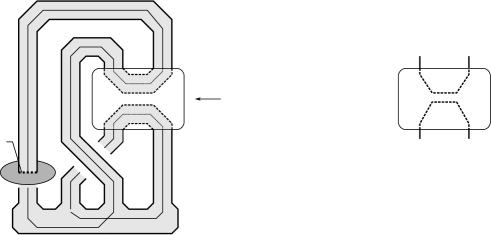
Figure 1. A spine tangle $T$ adapted to the cosmetic crossing

We call the framed tangle $T$ a spine tangle of $K$ adapted to the cosmetic crossing of a genus one knot $K$. Let $M=\begin{pmatrix}n&\ell\\ \ell&m\end{pmatrix}$ be the linking matrix of $T$, where $n$ (resp. $m$) is the framing of the strand $x$ (resp. $y$) and $\ell$ is the linking number of two strands of $T$.

Let $K^{\prime}$ be a knot obtained from $K$ by crossing change along the crossing disk $D$. Then $S$ gives rise to a Seifert surface $S^{\prime}$ of $K^{\prime}$ ([BFKP, Proposition 2.1]). $K^{\prime}$ has a spine tangle presentation $T^{\prime}$, so that $T^{\prime}$ and $T$ are the same as unframed tangles, and that the linking matrix of $T^{\prime}$ is $M^{\prime}=\begin{pmatrix}n\pm 1&\ell\\ \ell&m\end{pmatrix}$

With respect to the basis $\{a_{x},a_{y}\}$, the Seifert matrix $V$ of $K$ and the Seifert matrix $V^{\prime}$ of $K^{\prime}$ are given by

$$V=\begin{pmatrix}n&\ell\\ \ell\pm 1&m\end{pmatrix},\quad V^{\prime}=\begin{pmatrix}n\pm 1&\ell\\ \ell\pm 1&m\end{pmatrix}$$

respectively. Since $K$ and $K^{\prime}$ are the same knot,

$$\Delta_{K}(t)\doteq\det(V-tV^{T})\doteq\det(V^{\prime}-tV^{\prime}{}^{T})\doteq\Delta_{K^{\prime}}(t).$$

By direct computation, this implies that

(2.1) $$m=0.$$

In particular, $K$ is algebraically slice.

3. 2-loop polynomial of genus one knot

Here we quickly review the 2-loop polynomial. For details, see [Oht]. Let $\mathcal{B}$ be the space of open Jacobi diagram. For a knot $K$ in $S^{3}$, let $Z^{\sigma}(K)\in\mathcal{B}$ be the Kontsevich invariant of $K$, viewed so that it takes value in $\mathcal{B}$ by composing the inverse of the Poincaré-Birkoff-Witt isomorphism $\sigma:\mathcal{A}(S^{1})\rightarrow\mathcal{B}$.

A Jacobi diagram whose edge is labeled by a power series $f(\hbar)=c_{0}+c_{1}\hbar+c_{2}\hbar^{2}+c_{3}\hbar^{3}+\cdots$ represents the Jacobi diagram

$$\raisebox{-11.38109pt}{ \begin{picture}(20.0,30.0)\put(2.0,0.0){\line(0,1){30.0}} \put(5.0,22.0){\scriptsize$f(\hbar)$} \end{picture} }=c_{0}\raisebox{-11.38109pt}{ \begin{picture}(10.0,30.0)\put(2.0,0.0){\line(0,1){30.0}} \end{picture} }+c_{1}\raisebox{-11.38109pt}{ \begin{picture}(10.0,30.0)\put(2.0,0.0){\line(0,1){30.0}} \put(2.0,15.0){\line(1,0){10.0}} \end{picture} }+c_{2}\raisebox{-11.38109pt}{ \begin{picture}(10.0,30.0)\put(2.0,0.0){\line(0,1){30.0}} \put(2.0,12.0){\line(1,0){10.0}} \put(2.0,18.0){\line(1,0){10.0}} \end{picture} }+c_{3}\raisebox{-11.38109pt}{ \begin{picture}(10.0,30.0)\put(2.0,0.0){\line(0,1){30.0}} \put(2.0,9.0){\line(1,0){10.0}} \put(2.0,15.0){\line(1,0){10.0}} \put(2.0,21.0){\line(1,0){10.0}} \end{picture} }+\cdots$$

It is known that (the logarithm of) the Kontsevich invariant $Z^{\sigma}(K)$ is written in the following form [GaKr, Kri].

$$\log_{\sqcup}Z^{\sigma}(K) =\raisebox{-19.91692pt}{ \begin{picture}(140.0,60.0)\put(70.0,22.0){\oval(140.0,20.0)} \put(5.0,40.0){\footnotesize$\frac{1}{2}\log\left(\frac{\sinh(\hbar/2)}{\hbar/2}\right)-\frac{1}{2}\log(\Delta_{K}(e^{\hbar}))$} \end{picture} }+\sum_{i:\textrm{finite}}\raisebox{-22.76219pt}{ \begin{picture}(80.0,60.0)\put(40.0,25.0){\oval(80.0,50.0)} \put(0.0,25.0){\line(1,0){80.0}} \put(10.0,54.0){\footnotesize$p_{i,1}(e^{\hbar})/\Delta_{K}(e^{\hbar})$} \put(10.0,29.0){\footnotesize$p_{i,2}(e^{\hbar})/\Delta_{K}(e^{\hbar})$} \put(10.0,6.0){\footnotesize$p_{i,3}(e^{\hbar})/\Delta_{K}(e^{\hbar})$} \end{picture} }$$

$$\qquad+((\ell>2)\mbox{-loop parts}).$$

Here

• $\Delta_{K}(t)$ is the Alexander polynomial of $K$, normalized so that $\Delta_{K}(1)=1$ and $\Delta_{K}(t)=\Delta_{K}(t^{-1})$ hold.

• $\log_{\sqcup}$ is the logarithm with respect to the disjoint union product $\sqcup$ of $\mathcal{B}$, given by

  $$\log_{\sqcup}(1+D)=D-\frac{1}{2}D\sqcup D+\frac{1}{3}D\sqcup D\sqcup D+\cdots.$$

• $p_{i,j}(e^{\hbar})$ is a polynomial of $e^{\hbar}$.

Let

$$\Theta(t_{1},t_{2},t_{3};K)=\sum_{\varepsilon\in\{\pm 1\}}\sum_{\sigma\in S_{3}}p_{i,1}(t^{\varepsilon}_{\sigma(1)})p_{i,2}(t^{\varepsilon}_{\sigma(2)})p_{i,3}(t^{\varepsilon}_{\sigma(3)}).$$

Here $S_{3}$ is the symmetric group of degree $3$. The 2-loop polynomial $\Theta_{K}(t_{1},t_{2})\in\mathbb{Q}[t_{1}^{\pm 1},t_{2}^{\pm 1}]$ of a knot $K$ is defined by

$$\Theta_{K}(t_{1},t_{2})=\Theta(t_{1},t_{2},t_{3};K)|_{t_{3}=t_{1}^{-1}t_{2}^{-1}}.$$

The reduced 2-loop polynomial is a reduction of the $2$-loop polynomial defined by

$$\widehat{\Theta}_{K}(t)=\frac{\Theta_{K}(t,1)}{(t^{\frac{1}{2}}-t^{-\frac{1}{2}})^{2}}\in\mathbb{Q}[t^{\pm 1}].$$

In general, although Ohtsuki developed fundamental techniques and machineries that enable us to compute $\Theta_{K}(t_{1},t_{2})$, the computation of the 2-loop polynomial is much more complicated than the computation of the 1-loop part (i.e., the Alexander polynomial). Fortunately, when the knot has genus one, Ohtsuki proved a direct formula of $\Theta_{K}(t_{1},t_{2})$ [Oht, Theorem 3.1]. Consequently he gave the following formula of the reduced 2-loop polynomial of genus one knots.

Theorem 3.1.

[Oht, Corollary 3.5] Let $K$ be a genus one knot expressed by using a framed 2-tangle $T$ as in Figure 1, and let $M=\begin{pmatrix}n&\ell\\ \ell&m\end{pmatrix}$ be the linking matrix of $T$. Then

$$\widehat{\Theta}_{K}(t) =\Bigl{(}(n+m)(d-\frac{nm}{2})-\ell(\ell+\frac{1}{2})(\ell+1)+12v_{3}\Bigr{)}\Bigl{(}-2-\frac{2d+1}{3}(t+t^{-1}-2)\Bigr{)}$$

$$\quad-4\left(mv_{2}^{xx}+nv_{2}^{yy}-(\ell+\frac{1}{2})v_{2}^{xy}+3v_{3}\right)\Delta_{K}(t)$$

Here

• $d=nm-\ell^{2}-\ell$. In particular, $\Delta_{K}(t)=dt+(1-2d)+dt^{-1}$.

• $v_{2}^{xx},v_{2}^{yy},v_{2}^{xy}$ (resp. $v_{3}$) are some integer-valued finite type invariant of $T$ whose degree is $2$ (resp. $3$), which do not depend on the framing.

4. Constraint for cosmetic crossings

We prove the Theorem 1.2 and Theorem 1.3 at the same time.

Theorem 4.1.

Let $K$ be a genus one knot. If $K$ admits a cosmetic crossing, then $\Delta_{K}(t)=1$ and $\lambda(\Sigma_{2}(K))-2w_{3}(K)\equiv 0\pmod{16}$.

Proof.

Assume that $K$ is a genus one knot admitting a cosmetic crossing. We express $K$ using a spine tangle $T$ adapted to the cosmetic crossing. Then as we have seen (2.1), the linking matrix of $T$ is $M=\begin{pmatrix}n&\ell\\ \ell&0\end{pmatrix}$. Moreover, for the knot $K^{\prime}$ obtained by the crossing change, $K^{\prime}$ has a spine tangle $T^{\prime}$ which is identical with $T$ as an unframed tangle with linking matrix is $M^{\prime}=\begin{pmatrix}n\pm 1&\ell\\ \ell&0\end{pmatrix}$.

Since the finite type invariants $v_{2}^{xx},v_{2}^{yy},v_{2}^{xy}$ and $v_{3}$ do not depend on the framing, by Theorem 3.1,

$$0 =\widehat{\Theta}_{K}(t)-\widehat{\Theta}_{K^{\prime}}(t)$$

$$=d(-2-\frac{2d+1}{3}(t+t^{-1}-2))-4v_{2}^{yy}(dt+(1-2d)+dt^{-1})$$

$$=d\left(-\frac{2d+1}{3}-4v_{2}^{yy}\right)t+\frac{d(4d-4)}{3}+4v_{2}^{yy}(2d-1)+d\left(-\frac{2d+1}{3}-4v_{2}^{yy}\right)t^{-1}.$$

Therefore

(4.1) $$d\left(-\frac{2d+1}{3}-4v_{2}^{yy}\right)=\frac{d(4d-4)}{3}+4v_{2}^{yy}(2d-1)=0.$$

If $d\neq 0$, by (4.1) $d=\frac{1}{4}$. Since $d\in\mathbb{Z}$, this is a contradiction so we conclude $d=0$ and $\Delta_{K}(t)=1$.

Then by (4.1), $d=0$ implies $v_{2}^{yy}=0$. Moreover, since $d=nm-\ell^{2}-\ell=-\ell(\ell+1)$, we get $\ell=0,-1$. Thus by Theorem 3.1, the reduced 2-loop polynomial is

$$\widehat{\Theta}_{K}(t)=12v_{3}\left(-2-\frac{1}{3}(t+t^{-1}-2)\right)-4\left(-\left(\ell+\frac{1}{2}\right)v_{2}^{xy}-3v_{3}\right)$$

hence

$$\widehat{\Theta}_{K}(1)=-12v_{3}+4\left(\ell+\frac{1}{2}\right)v_{2}^{xy},\ \widehat{\Theta}_{K}(-1)=4v_{3}+4\left(\ell+\frac{1}{2}\right)v_{2}^{xy}.$$

On the other hand, by [Oht, Proposition 1.1]

$$\widehat{\Theta}_{K}(1)=2w_{3}(K),\quad\widehat{\Theta}_{K}(-1)=-\frac{1}{12}V^{\prime}_{K}(-1)V_{K}(-1).$$

Since $\Delta_{K}(-1)=V_{K}(-1)=1$, by Mullins’ formula of the Casson-Walker invariant $\lambda_{w}$ of the double branched coverings [Mul],

$$\lambda_{w}(\Sigma_{2}(K))=-\frac{V^{\prime}_{K}(-1)}{6V_{K}(-1)}+\frac{\sigma(K)}{4}$$

we get

$$\widehat{\Theta}_{K}(-1)=\frac{1}{2}\lambda_{w}(\Sigma_{2}(K)).$$

For an integral homology sphere, the Casson invariant $\lambda$ is twice of the Casson-Walker invariant $\lambda_{w}$ hence we conclude

$$\lambda(\Sigma_{2}(K))-2w_{3}(K) =\widehat{\Theta}_{K}(-1)-\widehat{\Theta}_{K}(1)=16v_{3}.$$

∎

Proof of Corollary 1.4.

The reduced $2$-loop polynomial of genus pretzel knots $P(p,q,r)$ was given in [Oht, Example 3.6]. In particular, for $K=P(4k+1,4k+3,-(2k+1))$, $\widehat{\Theta}_{K}(1)$ and $\widehat{\Theta}_{K}(-1)$ are given by

$$\widehat{\Theta}_{K}(1)=-\frac{1}{8}(4k+2)(4k+4)(-2k),\widehat{\Theta}_{K}(-1)=-\frac{1}{24}(4k+2)(4k+4)(-2k)$$

hence

$$\lambda(\Sigma_{2}(K))-2w_{3}(K) =\widehat{\Theta}_{K}(-1)-\widehat{\Theta}_{K}(1)=\frac{1}{12}(4k+2)(4k+4)(-2k)$$

$$=-16\frac{(2k+1)(k+1)k}{12}.$$

When $k\equiv 1,2\pmod{4}$, $\frac{(2k+1)(k+1)k}{12}\not\in\mathbb{Z}$ hence $K$ does not admit cosmetic crossing by Theorem 1.3. ∎

References

- [BFKP] C. Balm, S. Friedl, E. Kalfagianni, and M. Powell, Cosmetic crossings and Seifert matrices, Comm. Anal. Geom. 20 (2012), 235–253.
- [BaKa] C. Balm and E. Kalfagianni, Knots without cosmetic crossings, Topology Appl. 207 (2016), 33–42.
- [GaKr] S. Garoufalidis and A. Kricker, A rational noncommutative invariant of boundary links, Geom. Topol. 8 (2004), 115–204.
- [Kal] E. Kalfagianni, Cosmetic crossing changes of fibered knots, J. reine angew. Math. 669 (2012), 151–164.
- [Kir] R. Kirby (ed). Problems in low-dimensional topology, Edited by Rob Kirby. AMS/IP Stud. Adv. Math., 2.2, Geometric topology (Athens, GA, 1993), 3–473, Amer. Math. Soc., Providence, RI, 1997.
- [Kri] A. Kricker, The lines of the Kontsevich integral and Rozansky’s rationality conjecture, arXiv:math/0005284.
- [LiMo] T. Lidman and A. Moore, Cosmetic surgery in L-spaces and nugatory crossings, Trans. Amer, Math. Soc. 369 (2017), 3639–3654.
- [Mul] D. Mullins, The generalized Casson invariant for 2-fold branched covers of and the Jones polynomial, Topology 32 (1993), 419–438.
- [Oht] T. Ohtsuki, On the 2-loop polynomial of knots, Geom. Topol. 11 (2007), 1357–1475.
- [Tor] I. Torisu, On nugatory crossings for knots, Topology Appl. 92 (1999), 119–129.