Rouse model with fluctuating internal friction

Abstract

A coarse-grained bead-spring-dashpot chain model with the dashpots representing the presence of internal friction, is solved exactly numerically, for the case of chains with more than two beads. Using a decoupling procedure to remove the explicit coupling of a bead’s velocity with that of its nearest neighbors, the governing set of stochastic differential equations are solved with Brownian dynamics simulations to obtain material functions in oscillatory and steady simple shear flow. Simulation results for the real and imaginary components of the complex viscosity have been compared with the results of previously derived semi-analytical approximations, and the difference in the predictions are seen to diminish with an increase in the number of beads in the chain. The inclusion of internal friction results in a non-monotonous variation of the viscosity with shear rate, with the occurrence of continuous shear-thickening following an initial shear-thinning regime. The onset of shear-thickening in the first normal stress coefficient is pushed to lower shear rates with an increase in the internal friction parameter.

I Introduction

The presence of an additional mode of dissipation in polymer molecules arising from intramolecular interactions, denoted as internal friction or internal viscosity (IV) Kuhn and Kuhn (1945); Booij and van Wiechen (1970); de Gennes (1979); Manke and Williams (1985, 1988); Dasbach, Manke, and Williams (1992); Gerhardt and Manke (1994), has been invoked to reconcile the high values of dissipated work observed in force spectroscopic measurements on single molecules Murayama, Wada, and Sano (2007); Alexander-Katz, Wada, and Netz (2009); Schulz, Miettinen, and Netz (2015); Kailasham, Chakrabarti, and Prakash (2020), the steepness of the probability distribution of polymer extensions in coil-stretch transitions observed in turbulent flow Vincenzi (2021), and the dampened reconfiguration kinetics of biopolymers Arbe et al. (2001); Poirier and Marko (2002); Khatri et al. (2007); Qiu and Hagen (2004); Soranno et al. (2012); Samanta and Chakrabarti (2013); Samanta, Ghosh, and Chakrabarti (2014); Samanta and Chakrabarti (2016); Sashi, Ramakrishna, and Bhuyan (2016); Soranno et al. (2017); Das and Makarov (2018); Mondal, Adhikari, and Sharma (2020); Subramanian et al. (2020). The discontinuous jump in the stress in polymer solutions upon the inception or cessation of flow Liang and Mackay (1993); Orr and Sridhar (1996) has also been attributed to internal friction. Given its wide-ranging impact, a careful investigation of the consequences of the presence of internal friction is essential. As shown in Fig. 1, the bead-spring-chain model Bird et al. (1987); Öttinger (1996), widely used to describe the dynamics of flexible polymer chains, has been modified to include a dashpot in parallel with each spring to account for internal friction effects Booij and van Wiechen (1970); Bird et al. (1987); Ravi Prakash (1999). The dashpot provides a restoring force proportional to the relative velocity between adjacent beads, and acts along the connector vector joining these beads. The machinery for the solution of coarse-grained polymer models through Brownian dynamics (BD) simulations is well-established Bird et al. (1987); Öttinger (1996): the equation of motion for the connector vector velocities is combined with an equation of continuity in probability space to obtain a Fokker-Planck equation for the system, and the equivalent stochastic differential equation is integrated numerically. The inclusion of IV, however, results in a coupling of connector vector velocities and precludes a trivial application of the usual procedure for all but the simplest case of a dumbbell. By expanding the scope of an existing methodology for velocity-decoupling Manke and Williams (1988), the exact set of governing stochastic differential equations for a bead-spring-dashpot chain with $N_{\mathrm{b}}$ beads, and its numerical solution using BD simulations is presented here. The thermodynamically consistent Schieber and Öttinger (1994) stress tensor expression for this model is derived, and material functions in simple shear and oscillatory shear flows have been calculated. The decoupling procedure and the governing equations for bead-spring-chain dashpots derived in this work holds for arbitrary spring force laws. However, attention is restricted to the case of Hookean springs for the purposes of comparison with available approximate results in the literature Manke and Williams (1988); Dasbach, Manke, and Williams (1992); Schieber (1993) where appropriate.

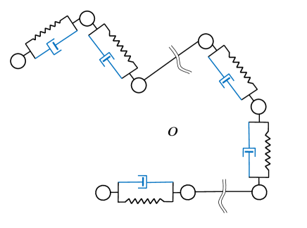
Figure 1: Representation of a polymer chain as a sequence of beads connected by spring-dashpots. The Hookean spring constant associated with each spring is $H$, and the damping coefficient of each dashpot is $K$.

Given that the phenomenon of internal friction has both rheological and biophysical consequences, it is instructive to briefly discuss the chronology of research on this topic by both these communities, before presenting the results. In the rheology community, the expression for the internal viscosity force law in two dimensions was first introduced by Kuhn and Kuhn (1945) in 1945. The three-dimensional analogue given by Booij and van Wiechen (1970) in 1970 has since been used by many others Manke and Williams (1988); Dasbach, Manke, and Williams (1992); Schieber (1993); Wedgewood (1993); Kailasham, Chakrabarti, and Prakash (2018) in the modeling and simulation of coarse-grained polymer models with an additional, solvent-viscosity-independent source of dissipation, and is also used in the present work. The effect of this additional mode of dissipation on conformational transitions in biomolecules was observed experimentally in the early 1990s Ansari et al. (1992), with the term “internal friction” predominantly used in the biophysics literature to refer to this phenomenon. A popularly used theoretical framework for the analysis of internal friction effects in experiments and simulations Soranno et al. (2012); Schulz et al. (2012); Ameseder et al. (2018) on biopolymers is the Rouse model with internal friction (RIF), developed by McLeish and coworkers Khatri and McLeish (2007); Khatri et al. (2007). The form of the internal friction force law in the RIF model is different from that used for the internal viscosity force in the rheology literature. We have recently shown [Ref. Kailasham, Chakrabarti, and Prakash (2021), under review] that the force law in the RIF model is essentially a preaveraged treatment of the exact internal viscosity force law which accounts for fluctuations. We rationalize in Ref. Kailasham, Chakrabarti, and Prakash (2021) that the form of the internal viscosity force law used in the rheology literature may therefore be considered as “fluctuating internal friction”, and that the same theoretical framework may consequently be applied for studying both rheological and biophysical phenomena. The present work considers only fluctuating internal friction, and the phrase “internal friction” or “IV” is henceforth used interchangeably and unambiguously.

It is worthwhile briefly surveying the methods employed in the past, before turning our attention to the solution proposed in the present work. Booij and van Wiechen Booij and van Wiechen (1970) used perturbation analysis to expand the configurational distribution function of a Hookean spring-dashpot in terms of the internal friction parameter, $\varphi=K/\zeta$, which is the ratio of the dashpot’s damping coefficient, $K$, to the bead friction coefficient, $\zeta$, and predicted optical and rheological properties in the presence of steady shear flow. On the other hand, Williams and coworkers offered a semi-analytical approximate solution for the stress-jump Manke and Williams (1988) of bead-spring-dashpot-chains with an arbitrary number of beads, using a decoupling procedure which is discussed at length later in this paper. They also obtained predictions for the complex viscosity of such chains by writing the configurational distribution function as a series expansion in strain Dasbach, Manke, and Williams (1992). While the approach of Booij and van Wiechen (1970) is restricted to small values of the internal friction parameter, the solutions proposed by Williams and coworkers Manke and Williams (1988); Dasbach, Manke, and Williams (1992) are applicable only in the linear viscoelastic regime. The transient variation and steady-state values of viscometric functions of bead-spring-dashpot chains with arbitrary chain-length in shear flow have been predicted Bazúa and Williams (1974); Manke and Williams (1989) using the linearized rotational velocity Cerf (1957); R. Cerf (1969); Peterlin (1967) (LRV) approximation for the internal friction force. As mentioned previously, the form of the internal friction force proposed by Booij and van Wiechen Booij and van Wiechen (1970) and Williams and coworkers Manke and Williams (1988); Dasbach, Manke, and Williams (1992) posits that the restoring force due to the dashpot is proportional to the relative velocity between adjacent beads projected along the tie-line joining these beads. The LRV approximation, however, assumes a more complicated dependence of the dashpot restoring force, and consequently results in erroneous predictions for the stress jump as indicated by Manke and Williams (1988). Furthermore, the LRV approximation predicts that the imaginary component of the complex viscosity, $\eta^{\prime\prime}$, vanishes at large values of internal friction parameter, $\varphi$, for all frequencies.  Dasbach, Manke, and Williams (1992) showed this prediction to be in stark contrast to their semi-analytical approximation which predicts a limiting non-zero value for $\eta^{\prime\prime}$ as $\varphi\to\infty$. The LRV approximation was consequently established as being incorrect Booij and van Wiechen (1970); Manke and Williams (1988); Dasbach, Manke, and Williams (1992) and its use was subsequently discarded. For the simplest case of a single-mode dumbbell-dashpot, it is straightforward to formulate the governing Fokker-Planck equation and obtain its equivalent stochastic differential equation. Both linear viscoelastic properties Hua and Schieber (1995); Kailasham, Chakrabarti, and Prakash (2018) and viscometric functions in steady-shear flow Hua, Schieber, and Manke (1996); Kailasham, Chakrabarti, and Prakash (2018) have been calculated for this model using Brownian dynamics (BD) simulations, for arbitrary values of the internal friction parameter. The single-mode spring-dashpot model has also been solved using a Gaussian approximation for the distribution function Schieber (1993); Sureshkumar and Beris (1995). Upon comparison against exact BD simulation results, it was found that the Gaussian approximation (GA) offers accurate predictions of linear viscoelastic properties, but is unable to predict the shear-thickening of viscosity Hua and Schieber (1995); Kailasham, Chakrabarti, and Prakash (2018) predicted by the exact model. Furthermore, the predictions for the stress jump in the start up of shear flow, obtained from BD simulations on the exact model, the Gaussian approximation, and the semi-analytical treatment of Manke and Williams agree with one another Hua and Schieber (1995).

Fixman Fixman (1988) has shown that the effects of bond length and bond angle constraints in stiff polymer models may be sufficiently mimicked by a Rouse/Zimm-like chain with internal friction. A preaveraged form of the internal friction force was chosen for analytical tractability, and this simplified model yields predictions for equilibrium and linear viscoelastic properties, such as the bond-vector correlations and storage and loss moduli, that are in reasonable agreement with that of stiff polymer chains. In the RIF model mention above, the standard continuum Rouse model is modified to include a rate-dependent dissipative force that resists changes in the curvature of the space-curve representing the polymer molecule. An expression for the autocorrelation of the end-to-end vector of the chain, and a closed-form expression for the dynamic compliance of the chain has been derived by them Khatri and McLeish (2007). The RIF model, and its variants Cheng, Hawk, and Makarov (2013); Samanta, Ghosh, and Chakrabarti (2014); Samanta and Chakrabarti (2016) which include excluded volume interactions and preaveraged hydrodynamic interactions, has been widely used to interpret the results of experiments and simulations on conformational transitions in biopolymers Soranno et al. (2012); Schulz et al. (2012); Ameseder et al. (2018), where the polymers do not experience a flow profile. To the best of our knowledge, an expression for the transient evolution of the mean-squared end-to-end vector of an RIF chain in flow is unknown, as are the viscometric functions. A thorough test of the accuracy of the preaveraging approximation, by comparing model predictions for observables at equilibrium and in flow, against exact BD simulations which account for fluctuations in internal friction, will be published as a separate study Kailasham, Chakrabarti, and Prakash (2021).

There currently exists no methodology that is able to predict both linear viscoelastic properties and viscometric functions in shear flow for bead-spring-dashpot chains with arbitrary number of beads and magnitude of internal friction parameter. We address this deficiency by solving the bead-spring-dashpot chain problem exactly. We compare BD simulation results for the stress jump and complex viscosity against approximate analytical predictions given in Ref. 5 and Ref. 6, respectively, and present steady-state results for viscometric functions in simple shear flow for the general case of $N_{\text{b}}>2$, for the first time.

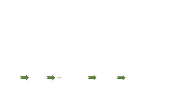
Figure 2: Schematic of three-step decoupling methodology introduced in Manke and Williams Manke and Williams (1988).

A crucial step in our methodology is the decoupling of the connector vector velocities of neighboring beads. Stripping away all physical detail, the decoupling problem may be stated as follows: given a “generating equation" for some function ${\mathcal{S}}_{j}$ of $\{{X}_{1},{X}_{2},\dots,{X}_{N}\}$, which is of the form

$${\mathcal{S}}_{j}=d_{j-1}{\mathcal{S}}_{j-1}+e_{j+1}{\mathcal{S}}_{j+1}+\xi\left({X}_{1},{X}_{2},\dots,{X}_{N}\right)$$ (1)

where $j\in[1,N]$, and $\left\{\xi,d_{j},e_{j}\right\}$ are some arbitrary functions of the ${X}_{i}$, is it possible to write an expression for ${\mathcal{S}}_{j}$ solely in terms of the ${X}_{i}$ that does not explicitly depend on any other ${\mathcal{S}}_{i}$? Manke and Williams Manke and Williams (1988) have proposed a three-step procedure for the solution of this problem. As the first step, the equation for ${\mathcal{S}}_{j}$ is successively substituted into ${\mathcal{S}}_{j+1}$, starting from $j=1$. At the end of this forward substitution step, an equation for ${\mathcal{S}}_{j}$ is obtained that only depends explicitly on ${\mathcal{S}}_{j+1}$ and ${X}_{i}$ with $1\leq\,i\leq\,j$. The second step is a backward substitution, where the equation for ${\mathcal{S}}_{j}$ is successively substituted into ${\mathcal{S}}_{j-1}$, starting from $j=N$. This results in an expression for ${\mathcal{S}}_{j}$ that only depends explicitly on ${\mathcal{S}}_{j-1}$ and ${X}_{i}$ with $j\leq\,i\leq\,N$. Finally, upon combining the results from the forward and backward substitution procedures, the decoupling procedure is completed, resulting in ${\mathcal{S}}_{j}=\mathcal{A}_{j}\xi\left({X}_{1},{X}_{2},\dots,{X}_{N}\right)$ where $\mathcal{A}_{j}$ is defined recursively in terms of $d$ and $e$. While the decoupling methodology developed by Manke and Williams has been adopted in the present work, we differ significantly in the generating equation which is subjected to the decoupling procedure. A schematic representation of the decoupling methodology is displayed in Fig. 2, and the differences between the use of the methodology in the present work and that of Manke and Williams Manke and Williams (1988) is discussed briefly in Sec. II. In order to illustrate the use of the decoupling methodology, its application to a three-spring chain with internal friction is discussed in detail in Appendix A. This simple case permits the demonstration of the essential aspects of the methodology, without excessive algebra.

The rest of the paper is structured as follows. Sec. II describes the bead-spring-dashpot chain model for a polymer, presents the governing stochastic differential equations and the stress tensor expression, and contains simulation details pertaining to the numerical integration of the governing equations. Sec. III, which is a compilation of our results and the relevant discussion, is divided into three sections; Sec. III.1 deals with code validation, Sec. III.2 presents results for the complex viscosity calculated from oscillatory shear flow simulations, and Sec. III.3 contains results for steady shear viscometric functions,. We conclude in Sec. IV. Appendix A contains the detailed steps showing the implementation of the decoupling algorithm represented in Fig. 2 to a three-spring chain, and the derivation of the governing Fokker-Planck equation for the system. Additional details pertaining to the methodology developed in the present work and its implementation are provided in the Supplementary Material, and its various sections are referenced appropriately in the text below.

II Governing Equation and simulation details

We consider $N_{\text{b}}$ massless beads, each of radius $a$, joined by $N\equiv\left(N_{\text{b}}-1\right)$ Hookean springs, with a dashpot in parallel with each spring, as shown in Fig. 1. The position of the $i^{\text{th}}$ bead is denoted as $\bm{r}_{i}$, and the connector vector joining adjacent beads is represented as $\bm{Q}_{i}\equiv\bm{r}_{i+1}-\bm{r}_{i}$. The centre-of-mass of the chain is denoted by $\boldsymbol{r}_{\text{c}}\equiv\left(1/N_{\text{b}}\right)\sum_{\nu=1}^{N_{\text{b}}}\boldsymbol{r}_{\nu}$. As will be seen shortly, in the absence of hydrodynamic interactions (HI), the inclusion of IV results in an explicit coupling of the connector vector velocities between nearest neighbors, and these velocities may be decoupled using the procedure suggested by Manke and Williams Manke and Williams (1988). The simultaneous inclusion of fluctuating hydrodynamic interactions and internal friction, however, results in a one-to-all coupling of the connector vector velocities, which renders the problem intractable using the Manke and Williams approach Manke and Williams (1988). It is noted, however, that in dumbbell models with internal friction, hydrodynamic interactions significantly magnify the stress jump and perceptibly affect the transient viscometric functions Kailasham, Chakrabarti, and Prakash (2018). Coarse-grained polymer models which incorporate both fluctuating hydrodynamic interactions and internal friction are currently unsolved for the $N_{\text{b}}>2$ case. In this work, we restrict our attention to freely-draining bead-spring-dashpot chains.

The chain, as shown in Fig. 1, is suspended in a Newtonian solvent of viscosity $\eta_{\text{s}}$ where the velocity $\bm{v}_{\text{f}}$ at any location $\bm{r}_{\text{f}}$ in the fluid is given by $\bm{v}_{\text{f}}(\bm{r}_{\text{f}},t)\equiv\,\bm{v}_{0}+\boldsymbol{\kappa}(t)\cdot\bm{r}_{\text{f}}$, where $\bm{v}_{0}$ is a constant vector, and the transpose of the velocity gradient tensor is denoted as $\boldsymbol{\kappa}\equiv\left(\nabla\bm{v}_{\text{f}}\right)^{T}$. The chain is assumed to have completely equilibrated in momentum space, and its normalized configurational distribution function at any time $t$ is specified as $\Psi\equiv\Psi\left(\bm{r}_{1},\bm{r}_{2},...,\bm{r}_{{N_{\text{b}}}},t\right)=\left(1/\mathcal{Z}\right)\exp\left[-\phi/k_{B}T\right]$, where $\phi$ denotes the intramolecular potential energy stored in the springs joining the beads, $k_{B}$ is Boltzmann’s constant, $T$ the absolute temperature, and $\mathcal{Z}=\int\exp\left[-\phi/k_{B}T\right]d\bm{Q}_{1}d\bm{Q}_{2}\dots\,d\bm{Q}_{N}$. It is worth noting that the equilibrium configurational distribution function is unperturbed by the inclusion of internal friction. The spring force in the $k^{\text{th}}$ connector vector is denoted as $\bm{F}^{\text{s}}_{k}=\partial\phi/\partial\bm{Q}_{k}$, with $\bm{F}^{\text{s}}_{k}=H\bm{Q}_{k}$ for a Hookean spring where $H$ is the spring constant. The expression for the IV force, $\bm{F}^{\text{IV}}_{k}$, in the $k^{\text{th}}$ connector vector may be written as

$$\bm{F}^{\text{IV}}_{k}=K\left(\dfrac{\bm{Q}_{k}\bm{Q}_{k}}{Q_{k}^{2}}\right)\cdot\llbracket\dot{\bm{Q}}_{k}\rrbracket,$$ (2)

where $K$ is the damping coefficient of the dashpot, and $\llbracket\dots\rrbracket$ denotes an average over momentum-space. Within the framework of polymer kinetic theory Bird et al. (1987), the Fokker-Planck equation for the configurational distribution function is obtained by combining a force-balance on the beads (or connector vectors) with a continuity equation in probability space. The force-balance mandates that the sum of: (i) the internal friction force due to the dashpot, (ii) the restoring force from the Hookean spring, (iii) the random Brownian force arising from collisions with solvent molecules, and (iv) the hydrodynamic force which represents the solvent’s resistance to the motion of the bead, equals zero. It is convenient to work with connector vectors, rather than bead positions, for models with internal friction, and the following equations have been derived in Ref. 30 for the momentum-averaged velocity of the $k^{\text{th}}$ connector vector and the centre-of-mass, respectively,

$$\llbracket\dot{\bm{Q}}_{k}\rrbracket =\boldsymbol{\kappa}\cdot\bm{Q}_{k}-\dfrac{1}{\zeta}\sum^{N}_{l=1}\bm{{A}}_{kl}\cdot\Biggl{(}\uline{k_{B}T\dfrac{\partial\ln\Psi}{\partial\bm{Q}_{l}}}+\dashuline{\dfrac{\partial\phi}{\partial\bm{Q}_{l}}}$$

$$+K\dfrac{\bm{Q}_{l}\bm{Q}_{l}}{\bm{Q}^{2}_{l}}\cdot\llbracket\dot{\bm{Q}}_{l}\rrbracket\Biggr{)}$$ (3)

$$\llbracket\dot{\bm{r}}_{\text{c}}\rrbracket =\bm{v}_{0}+\boldsymbol{\kappa}\cdot\bm{r}_{\text{c}}+\left(\dfrac{1}{N_{\text{b}}\zeta}\right)\sum^{N}_{k=1}\Biggl{[}k_{B}T\dfrac{\partial\ln\Psi}{\partial\bm{Q}_{k}}+\dfrac{\partial\phi}{\partial\bm{Q}_{k}}$$

$$+K\dfrac{\bm{Q}_{k}\bm{Q}_{k}}{Q^{2}_{k}}\cdot\llbracket\dot{\bm{Q}}_{k}\rrbracket\Biggr{]}$$ (4)

where $\zeta\coloneqq 6\pi\eta_{\text{s}}a$ is the monomeric friction coefficient, and ${\bm{A}}_{kl}={A}_{kl}\bm{\delta}$ where ${A}_{kl}$ are the elements of the Rouse matrix, given by

$$A_{kl}=\left\{\begin{array}[]{ll}2;&k=l\\[15.0pt] -1;&|k-l|=1\\[15.0pt] 0;&\text{otherwise}.\end{array}\right.$$ (8)

As seen from Eq. (II), there is an explicit coupling between the velocity of the $k^{\text{th}}$ connector vector and its nearest neighbors which precludes a straightforward substitution into the equation of continuity for the configurational distribution function. This velocity-coupling may be removed by applying the decoupling scheme described in Fig. 2, to obtain the governing Fokker-Planck equation for the system, as shown in Section SII of the Supplementary Material. The crucial difference between the equation of motion for the connector vector used in the present work [Eq. (II)], and that used by Manke and Williams can be understood by considering the solid and dashed underlined terms on the RHS of Eq. (II), which represent the Brownian and spring force contributions, respectively. Manke and Williams Manke and Williams (1988) were concerned only with the evaluation of the stress-jump, which occurs instantaneously upon the inception of flow. Since the Brownian and spring forces exactly balance each other at equilibrium, i.e., $k_{B}T\left(\partial\ln\Psi_{\text{eq}}\right/\partial\bm{Q}_{l})+\left(\partial\phi/\partial\bm{Q}_{l}\right)=0$, Manke and Williams Manke and Williams (1988) ignore both these forces in their equation of motion. Here, however, we aim to find the exact governing equation that is valid both near and far away from equilibrium, and have consequently retained both the underlined terms in the force-balance equation. This is essentially the source of the difference between the two decoupling methodologies.

Using $l_{H}\equiv\sqrt{k_{B}T/H}$ and $\lambda_{H}\equiv\zeta/4H$ as the length- and time-scales, respectively, and denoting dimensionless variables with an asterisk as superscript, the dimensionless form of the Fokker-Planck equation is given as

$$\dfrac{\partial\psi^{*}}{\partial t^{*}} =-\sum_{j=1}^{N}\dfrac{\partial}{\partial\bm{Q}^{*}_{j}}\cdot\Biggl{\{}\Biggl{[}\boldsymbol{\kappa}^{*}\cdot\bm{Q}^{*}_{j}-\left(\dfrac{\varphi}{1+2\varphi}\right)\sum^{N}_{k=1}{\bm{U}}_{jk}\cdot\left(\boldsymbol{\kappa}^{*}\cdot\bm{Q}^{*}_{k}\right)-\dfrac{1}{4}\sum^{N}_{k=1}\widehat{\bm{A}}_{jk}\cdot\bm{F}^{*\text{s}}_{k}$$ (9)

$$-\dfrac{1}{4}\left(\dfrac{\varphi}{1+2\varphi}\right)\sum_{k=1}^{N}\dashuline{\dfrac{\partial}{\partial\bm{Q}^{*}_{k}}\cdot\bm{V}_{jk}^{T}}\Biggr{]}\psi^{*}\Biggr{\}}+\dfrac{1}{4}\sum^{N}_{j,k=1}\dfrac{\partial}{\partial\bm{Q}^{*}_{j}}\dfrac{\partial}{\partial\bm{Q}^{*}_{k}}:\left[\widehat{\bm{A}}_{jk}^{T}\psi^{*}\right]$$

where the dimensionless tensors $\bm{U}_{jk},\bm{V}_{jk},\text{and}\,\widehat{\boldsymbol{A}}_{jk}\equiv\boldsymbol{A}_{jk}-({\varphi}/{1+2\varphi})\boldsymbol{V}_{jk}$ are functions of the internal friction parameter, with definitions given in the Supplementary Material. In the absence of internal friction, both $\bm{U}_{jk},\text{and}\,\bm{V}_{jk}$ reduce to $\bm{0}$, and $\widehat{\bm{A}}_{jk}$ becomes the Rouse matrix. For the special case of a dumbbell ($N=1$), it may be shown (as detailed in Sec. SII A of the Supplementary Material) that Eq. (9) is identical to the Fokker-Planck equations obtained in previous studies Hua and Schieber (1995); Kailasham, Chakrabarti, and Prakash (2018) on dumbbells with internal friction. In order to simplify the notation, it is convenient to rewrite the Fokker-Planck equation in terms of collective coordinates. We define

$$\widetilde{\bm{Q}}^{*}\equiv\left[\bm{Q}^{*}_{1},\,\bm{Q}^{*}_{2},\,...,\,\bm{Q}^{*}_{N}\right]\equiv\left[Q^{*1}_{1},Q^{*2}_{1},Q^{*3}_{1},Q^{*1}_{2},Q^{*2}_{2},\,...,\,Q^{*3}_{N}\right]$$ (10)

and write $\widetilde{Q}^{*}_{i}=Q^{*\beta}_{k}$, where $k=1,2,...,N$ and $\beta=1,2,3$ (represent Cartesian components in the $x,y,z$ directions, respectively), with $i$ related to $k$ and $\beta$ as $i=3\left(k-1\right)+\beta$. Similarly, $\widetilde{\bm{F}}^{*\text{s}}\equiv\left[\bm{F}^{*\text{s}}_{1},\,\bm{F}^{*\text{s}}_{2},\,...,\,\bm{F}^{*\text{s}}_{N}\right]$, and $\widetilde{\bm{v}}^{*}\equiv\left[\widehat{\bm{v}}^{*}_{1},\,\widehat{\bm{v}}^{*}_{2}\,...,\,\widehat{\bm{v}}^{*}_{N}\right]$, with $\widehat{\bm{v}}^{*}_{j}=\sum_{k=1}^{N}\left({\partial}/{\partial\bm{Q}^{*}_{k}}\right)\cdot\bm{V}_{jk}^{T}$. The dimensionless $N\times N$ block diffusion matrix $\bm{\mathcal{D}}$ is a function of the internal friction parameter, whose elements are the tensors $\widehat{\bm{A}}_{jk}$. The block matrix $\bm{\mathcal{K}}^{*}$ is defined such that its diagonal elements are given by the $3\times 3$ matrix $\boldsymbol{\kappa}^{*}$, and its off-diagonal blocks are $\bm{0}$. Lastly, the block matrix $\bm{\mathcal{U}}$ consists of the tensors $\bm{U}_{jk}$. In terms of these collective variables, the stochastic differential equation equivalent to Eq. (9), using Itô’s interpretation Öttinger (1996), is given by

$$\begin{split}d\widetilde{\bm{Q}}^{*}&=\Biggl{[}\bm{\mathcal{K}}^{*}\cdot\widetilde{\bm{Q}}^{*}-\left(\dfrac{\varphi}{1+2\varphi}\right){\bm{\mathcal{U}}}\cdot\left(\bm{\mathcal{K}}^{*}\cdot\widetilde{\bm{Q}}^{*}\right)-\dfrac{1}{4}\bm{\mathcal{D}}{\color[rgb]{0,0,1}(\varphi)}\cdot\widetilde{\bm{F}}^{*\text{s}}-\dfrac{1}{4}\left(\dfrac{\varphi}{1+2\varphi}\right)\widetilde{\bm{v}}^{*}\Biggr{]}dt^{*}+{\dfrac{1}{\sqrt{2}}}\bm{\mathcal{B}}{\color[rgb]{0,0,1}(\varphi)}\cdot d\bm{\widetilde{W}}^{*}\end{split}$$ (11)

where $\bm{\widetilde{W}}^{*}$ is a $3N-$dimensional Wiener process, and $\bm{\mathcal{B}}\cdot\bm{\mathcal{B}}^{T}=\bm{\mathcal{D}}$. The symmetricity and positive-definiteness of the diffusion matrix is established empirically in Section SII C of the Supplementary Material. The square-root of the diffusion matrix is found using Cholesky decomposition Press et al. (2007). While a higher-order semi-implicit predictor-corrector algorithm for the solution of dumbbells with internal friction exists in the literature Kailasham, Chakrabarti, and Prakash (2018), the complexity of the governing equations for the general case of $N_{\text{b}}>2$ precludes the construction of a higher order solver algorithm, and consequently, Eq. (11) is solved numerically using a simple explicit Euler method, as follows

$$\begin{split}\widetilde{\bm{Q}}^{*}\left(t_{n+1}\right)=&\widetilde{\bm{Q}}^{*}_{n}+\Biggl{[}\bm{\mathcal{K}}^{*}\left(t_{n}\right)\cdot\widetilde{\bm{Q}}^{*}\left(t_{n}\right)-\left(\dfrac{\varphi}{1+2\varphi}\right){\bm{\mathcal{U}}}\left(t_{n}\right)\cdot\left(\bm{\mathcal{K}}^{*}\left(t_{n}\right)\cdot\widetilde{\bm{Q}}^{*}\left(t_{n}\right)\right)-\dfrac{1}{4}\bm{\mathcal{D}}\left(t_{n}\right)\cdot\widetilde{\bm{F}}^{*\,\text{s}}\left(t_{n}\right)\\[5.0pt] &-\dashuline{\left(\dfrac{1}{4}\right)\left(\dfrac{\varphi}{1+2\varphi}\right)\widetilde{\bm{v}}^{*}\left(t_{n}\right)}\Biggr{]}\Delta t^{*}_{n}+{\dfrac{1}{\sqrt{2}}}\Delta\bm{\widetilde{S}}^{*}_{n}\end{split}$$ (12)

where $\Delta\bm{\widetilde{S}}^{*}_{n}=\bm{\mathcal{B}}\cdot\Delta\bm{\widetilde{W}}^{*}_{n}$.

It is observed from Eq. (11) that the inclusion of internal friction modifies both the drift and the diffusion (noise) components of the governing stochastic differential equation. Since the Hamiltonian of the system is unperturbed by internal friction, the equilibrium distribution function must be a solution to the Fokker-Planck equation [Eq. (9)] in the absence of the flow term, in order to satisfy the fluctuation-dissipation theorem. We have established (as detailed in Sec. SII B of the Supplementary Material) that the governing stochastic differential equation [Eq. (11)] satisfies the fluctuation-dissipation theorem by checking that the probability distribution of the end-to-end vector for a five-bead Rouse chain with internal friction at equilibrium, obtained by numerically integrating Eq. (12) with $\bm{\mathcal{K}}^{*}=\bm{0}$, agrees with the analytical expression.

In order to relate the time-evolution of the connector vectors to macroscopically observable rheological properties, it is necessary to specify an appropriate stress tensor expression for the model discussed above. The formal, thermodynamically consistent stress tensor expression for free-draining models with internal friction may be obtained using the Giesekus expression Schieber and Öttinger (1994), as follows

$$\begin{split}{\boldsymbol{\tau}_{\text{p}}}&=\dfrac{n_{\text{p}}\zeta}{2}\left<\sum_{j=1}^{N}\sum_{k=1}^{N}{\mathscr{C}_{jk}}\bm{Q}_{j}\bm{Q}_{k}\right>_{(1)}=\dfrac{n_{\text{p}}\zeta}{2}\left[\dfrac{d}{dt}\left<\sum_{j,k}{\mathscr{C}_{jk}}\bm{Q}_{j}\bm{Q}_{k}\right>-\boldsymbol{\kappa}\cdot\left<\sum_{j,k}{\mathscr{C}_{jk}}\bm{Q}_{j}\bm{Q}_{k}\right>-\left<\sum_{j,k}{\mathscr{C}_{jk}}\bm{Q}_{j}\bm{Q}_{k}\right>\cdot\boldsymbol{\kappa}^{T}\right]\end{split}$$ (13)

where $\mathscr{C}_{jk}$ is the Kramers matrix Bird et al. (1987). Upon simplification following considerable algebra, as discussed in Sec. SIII of the Supplementary Material,

$$\begin{split}{\boldsymbol{\tau}_{\text{p}}}&=n_{\text{p}}k_{B}T\left(N_{\text{b}}-1\right)\boldsymbol{\delta}-n_{\text{p}}\left<\sum_{k=1}^{N_{\text{b}}-1}\bm{Q}_{k}\bm{F}^{\text{c}}_{k}\right>\end{split}$$ (14)

which is formally similar to the Kramers expression Bird et al. (1987), except that the force in the connector vector, $\bm{F}_{k}^{c}$, is redefined to include contributions from both the spring and the dashpot (also noted in Refs. [33; 31; 46] for Hookean dumbbells with IV), as follows,

$$\begin{split}\bm{F}^{\text{c}}_{k}&=\bm{F}^{\text{s}}_{k}+KC_{k}\bm{Q}_{k}\end{split}$$ (15)

where $C_{k}=\left({\bm{Q}_{k}\cdot\llbracket\dot{\bm{Q}}_{k}\rrbracket}/{Q^{2}_{k}}\right)$. Plugging Eq. (15) into Eq. (14) and using the closed-form expression for $C_{k}$ as derived in the Supplementary Material, the dimensionless stress tensor expression is obtained as

$$\begin{split}\dfrac{\boldsymbol{\tau}_{\text{p}}}{n_{\text{p}}k_{B}T}&=\left(N_{\text{b}}-1\right)\boldsymbol{\delta}-\Biggl{[}\left<\sum_{k}\bm{Q}^{*}_{k}\bm{F}^{*\text{s}}_{k}\right>-\dfrac{1}{2}\left(\dfrac{\epsilon}{1+\epsilon}\right)\left<\sum_{k,l}\left(\bm{Q}^{*}_{k}\bm{F}^{*\text{s}}_{l}\right)\cdot\boldsymbol{\mu}_{kl}^{T}\right>\Biggr{]}-\dfrac{1}{2}\left(\dfrac{\epsilon}{1+\epsilon}\right)\Biggl{[}\left<\sum_{k}\boldsymbol{\mu}^{T}_{kk}\right>\\[15.0pt] &+\left<\sum_{k,l}\bm{Q}^{*}_{k}\dotuline{\dfrac{\partial}{\partial\bm{Q}^{*}_{l}}\cdot\boldsymbol{\mu}_{kl}^{T}}\right>\Biggr{]}-\left(\dfrac{2\epsilon}{1+\epsilon}\right)\boldsymbol{\kappa}^{*}:\left<\sum_{k,l}\dfrac{\chi^{(k)}_{l}\bm{Q}^{*}_{l}\bm{Q}^{*}_{l}\bm{Q}^{*}_{k}\bm{Q}^{*}_{k}}{Q^{*}_{l}Q^{*}_{k}}\right>\end{split}$$ (16)

where $\epsilon=2\varphi$, and the definitions of $\boldsymbol{\mu}_{kl}\,\text{and}\,\chi^{(k)}_{l}$ are provided in the Supplementary Material.

The bead-spring-dashpot chain is subjected to steady simple shear flow and small amplitude oscillatory shear flow. The flow tensor, $\boldsymbol{\kappa}$, for simple shear flow has the following form

$$\boldsymbol{\kappa}\equiv\boldsymbol{\kappa}^{*}\,\lambda^{-1}_{H}=\dot{\gamma}\begin{pmatrix}0&1&{0}\\ 0&0&0\\ {0}&0&0\end{pmatrix}$$ (17)

and is characterized by the following viscometric functions

$$\begin{split}\eta_{\text{p}}&=-\dfrac{\tau_{\text{p},xy}}{\dot{\gamma}}\\[5.0pt] \Psi_{1}&=-\left[\dfrac{\tau_{\text{p},xx}-\tau_{\text{p},yy}}{\dot{\gamma}^{2}}\right]\\[5.0pt] \Psi_{2}&=-\left[\dfrac{\tau_{\text{p},yy}-\tau_{\text{p},zz}}{\dot{\gamma}^{2}}\right]\end{split}$$ (18)

where $\tau_{\text{p},xy}$ refers to the $xy$ element of the stress tensor, and $\eta_{\text{p}}$, $\Psi_{1}$, and $\Psi_{2}$ denote the shear viscosity, the first normal stress coefficient, and the second normal stress coefficient, respectively. For small-amplitude oscillatory shear flow, we have

$$\boldsymbol{\kappa}=\dot{\gamma}_{0}\cos(\omega t)\begin{pmatrix}0&1&{0}\\ 0&0&0\\ {0}&0&0\end{pmatrix}$$ (19)

The material functions relevant to this flow profile, $\eta^{\prime}(\omega)$ and $\eta^{\prime\prime}(\omega)$, are given by

$$-\tau_{\text{p},xy}=\eta^{\prime}(\omega)\dot{\gamma}_{0}\cos(\omega t)+\eta^{\prime\prime}(\omega)\dot{\gamma}_{0}\sin(\omega t)$$ (20)

The variance reduction algorithm proposed by Wagner and Öttinger (1997) has been used in the evaluation of steady-shear viscometric functions at low shear rates ($\lambda_{H}\dot{\gamma}<1.0$), and for the calculation of oscillatory shear material functions at all frequencies reported in this work. Additional details pertaining to the variance reduction algorithm employed in the present work, and examples illustrating the efficacy of this technique have been provided in Section SIV Supplementary Material.

Where appropriate, the viscometric functions have either been scaled by their respective Rouse chain values, $\eta^{\text{R}}$ and $\Psi^{\text{R}}_{1}$, in steady shear flow, given as Bird et al. (1987)

$$\eta^{\text{R}}=n_{\text{p}}k_{B}T\lambda_{H}\left[\dfrac{N_{\text{b}}^{2}-1}{3}\right]$$ (21)

$$\Psi^{\text{R}}_{1}=2n_{\text{p}}k_{B}T\lambda^{2}_{H}\left[\dfrac{(N_{\text{b}}^{2}-1)(2N_{\text{b}}^{2}+7)}{45}\right]$$ (22)

or by the Rouse values of the real and imaginary portions of the complex viscosity given by Bird et al. (1987)

$${\left(\eta^{\prime}\right)^{\text{R}}} =n_{\text{p}}k_{B}T\sum_{j=1}^{N}\dfrac{\lambda_{j}}{1+\left(\lambda_{j}\omega\right)^{2}}$$ (23)

$${\left(\eta^{\prime\prime}\right)^{\text{R}}} =n_{\text{p}}k_{B}T\sum_{j=1}^{N}\dfrac{\lambda^{2}_{j}\omega}{1+\left(\lambda_{j}\omega\right)^{2}}$$ (24)

where $\lambda_{j}=2\lambda_{H}/a_{j}$, and $a_{j}=4\sin^{2}\left[j\pi/2N_{\text{b}}\right]$ are the eigenvalues of the Rouse matrix. Note that the dynamic viscosity, $\eta^{\prime}$, has the solvent viscosity contribution subtracted off and the convention is followed throughout this paper. Shear rates and angular frequencies are scaled using $\lambda_{\text{p}}\equiv\left(\eta^{\text{R}}/n_{\text{p}}k_{B}T\right)$, which is the characteristic relaxation time defined using the Rouse viscosity.

The initial configurations of the chains are drawn from an ensemble of Rouse chain configurations, since it is known that the equilibrium configurational probability distribution is unaffected by internal friction. The timestep width of the integrator is chosen after testing for convergence, by checking that the simulation output is independent of the choice of $\Delta t^{*}$, as explained in detail in Section SII D of the Supplementary Material. For example, at low values of the dimensionless shear rate or frequency$(<1.0)$, $\Delta t^{*}=10^{-2}$ is found to suffice, while higher shear rates or frequency necessitate the use of smaller time steps in the range of $10^{-5}$ to $10^{-3}$. The ensemble size for oscillatory shear simulations is chosen in the range of $\mathcal{O}(10^{3})$ to $\mathcal{O}(10^{5})$ trajectories, with the lower limit corresponding to simulations at smaller frequencies. Components of the complex viscosity are extracted by fitting Eq. (20) to three to five cycles of the observed stress, with the duration of a cycle given by $t^{*}_{\text{cycle}}=2\pi/\omega^{*}$. The ensemble size for steady-shear simulations is in the range of $\mathcal{O}(10^{4})$ to $\mathcal{O}(10^{5})$ trajectories.

The underlined divergence terms in Eqs. (9) and (16) may be calculated by two routes: analytically, using recursive functions as explained in Sec. SV of the Supplementary Material, or they can be calculated numerically. The connector vectors appearing in Eqs. (25)–(26) below are in their dimensionless form, with the asterisks omitted for the sake of clarity. The numerical route for the calculation of divergence is described below. Consider the general divergence,

$$\dfrac{\partial}{\partial\bm{Q}_{k}}\cdot\bm{\mathcal{G}}_{jk}=\sum_{\beta=1}^{3}\sum_{\gamma=1}^{3}\dfrac{\partial}{\partial{Q}^{\beta}_{k}}\left(\mathcal{G}^{\beta\gamma}_{jk}\right)\bm{e}_{\gamma}$$ (25)

where $\beta$ and $\gamma$ run over the three Cartesian indices, $\bm{\mathcal{G}}_{jk}$ is a configuration-dependent tensor, and $\bm{e}_{\gamma}$ is a unit vector. The computation of the divergence requires the calculation of nine gradient terms, which are evaluated using the central-difference approximation. One such evaluation is shown here as an example:

$$\begin{split}\dfrac{\partial}{\partial{Q}^{1}_{k}}\left(\mathcal{G}^{12}_{jk}\right)&=\dfrac{1}{2\Delta_{1}}\Biggl{[}\mathcal{G}^{12}_{jk}\left(Q_{k}^{1}+\Delta_{1},Q^{2}_{k},Q^{3}_{k}\right)\\ &-\mathcal{G}^{12}_{jk}\left(Q_{k}^{1}-\Delta_{1},Q^{2}_{k},Q^{3}_{k}\right)\Biggr{]}\end{split}$$ (26)

where $\Delta_{1}$ is the spatial discretization width along one Cartesian direction, representing the infinitesimal change in $Q_{k}^{1}$. The error in the evaluation of the gradient using this approximation scales as $\mathcal{O}\left(\Delta^{2}_{1}\right)$. We have validated that the divergences calculated numerically agrees with that obtained using recursive functions, and have chosen the numerical route in view of its faster execution time that is largely invariant with chain length. In numerical computations, we set $\Delta_{1}=\Delta_{2}=\Delta_{3}=\Delta_{\text{d}}=10^{-5}$, unless noted otherwise.

III Results

III.1 Code Validation

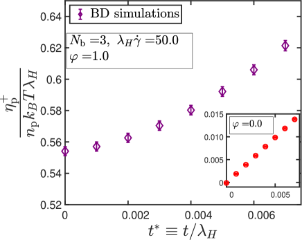
Figure 3: Time evolution of the shear viscosity of a three-bead Rouse chain with internal friction subjected to simple shear flow. The inset corresponds to the case without internal friction.

In Fig. 3, the transient viscosity of a three-bead Rouse chain with internal friction subjected to simple shear flow is plotted as a function of dimensionless time. An important rheological consequence of internal friction is the appearance of a discontinuous jump in viscosity at the inception of flow Manke and Williams (1988); Hua and Schieber (1995); Kailasham, Chakrabarti, and Prakash (2018). This phenomenon, called “stress jump" is not predicted by bead-spring-chain models without internal friction, as evident from the inset. The numerical value of the stress jump is taken to be the shear viscosity at the startup $(t^{*}=0)$ of simple shear flow.

In Fig. 4, the stress-jump observed for different chain lengths is plotted as a function of the dimensionless shear rate. It is observed that the stress jump is independent of the shear rate, in agreement with the theoretically expected trend Gerhardt and Manke (1994). The horizontal lines in the figure represent the approximate analytical values for the stress jump evaluated by Manke and Williams Manke and Williams (1988), and very good agreement is observed between the values estimated using the two approaches.

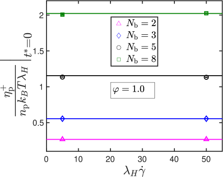
Figure 4: Stress jump as a function of dimensionless shear rate for various chain lengths and a fixed internal friction parameter of $\varphi=1.0$. Lines are approximate solutions by Manke and Williams Manke and Williams (1988). Error bars are smaller than symbol size.

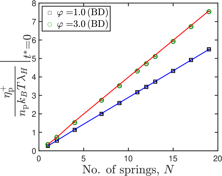
(a)

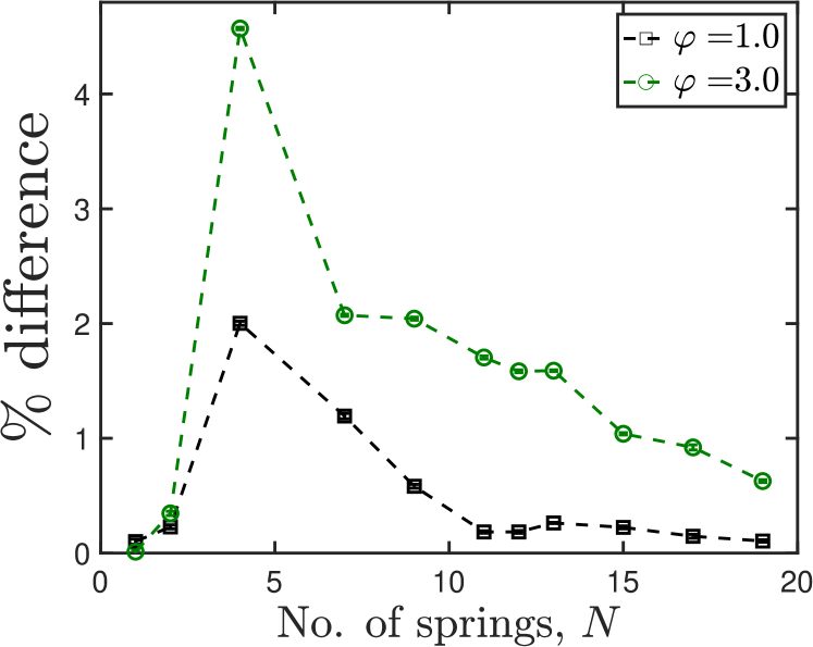
(b)

Figure 5: (a) Comparison of stress jump obtained using extrapolation of BD simulation data, and approximate solutions by Manke and Williams Manke and Williams (1988) indicated by solid lines. (b) Percentage difference between stress jump obtained using the two approaches, as a function of chain length. Dashed lines are drawn to guide the eye. Error bars are smaller than symbol size.

In Fig. 5 (a), the stress jump evaluated from BD simulations for two different values of the internal friction parameter is plotted as a function of the number of springs in the chain. The semi-analytical approximation of Manke and Williams Manke and Williams (1988) is found to compare favourably against the exact simulation result. Furthermore, it is observed that the stress jump scales linearly with number of springs in the chain, with the slope of the line dependent on the internal friction parameter. It is instructive to first understand the simplifying assumption made in Manke and Williams Manke and Williams (1988) before interpreting the data in Fig. 5 (b) where the percentage difference between the analytical and simulation results is plotted as a function of chain length at a fixed value of the internal friction parameter. Manke and Williams Manke and Williams (1988) assume that the terminal connector vectors and interior connector vectors contribute equally towards the stress jump. This assumption is necessary only for chains with $N>2$, because there is no distinction between a terminal and interior connector vector for a dumbbell ($N=1$), and the two connector vectors for the $N=2$ case are shown by Manke and Williams Manke and Williams (1988) to contribute identically to the total stress jump. It is likely that their assumption would most severely be tested in chains with fewer number of springs, where the terminal springs represent a larger fraction of the overall chain, and becomes progressively better with an increase in the number of springs. The expected trend is clearly borne out by Fig. 5 (b), where the deviation between the exact simulation result and the analytical value first increases (beyond $N=1$) and later decreases with the number of springs in the chain.

III.2 Complex viscosity from oscillatory shear flow

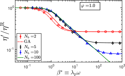
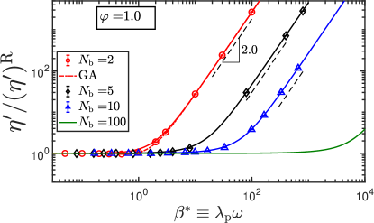
(a)	(b)
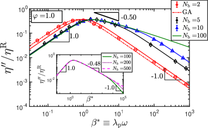
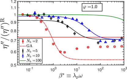
(c)	(d)

Figure 6: Plots of the real ($\eta^{\prime}$) and imaginary components ($\eta^{\prime\prime}$) of the complex viscosity, as a function of the scaled frequency, for a fixed value of the internal friction parameter and three different values for the number of beads in the chain. The solid lines are approximate solutions given in  Dasbach, Manke, and Williams (1992). The dash-dotted lines represent predictions obtained using the Gaussian approximation Schieber (1993). The lines in the inset of (c) are DMW results. Error bars are smaller than symbol size.

In Fig. 6, the material functions in oscillatory shear flow are plotted for a fixed value of the internal friction parameter, and varying number of beads in the chain. The exact BD simulation results, indicated by symbols, are compared against the the approximate prediction given by Dasbach, Manke, and Williams (1992) (DMW), shown as solid lines. Schieber Schieber (1993) has obtained predictions for $\eta^{\prime}$ and $\eta{{}^{\prime\prime}}$ for Hookean dumbbells ($N_{\text{b}}=2$) with internal viscosity, using a Gaussian approximation (GA), and these predictions have been shown using dash-dotted lines. The high-frequency-limiting value of $\eta^{\prime}$ obtained by GA agrees with that derived by Dasbach, Manke, and Williams (1992). Furthermore, while the functional form of $\eta^{\prime\prime}$ obtained by GA matches with the expression given by Dasbach, Manke, and Williams (1992), they differ in the sense that the GA predicts a $\varphi$-dependent rescaling of the frequency which is absent in the latter work.

As seen from Fig. 6 (a), the inclusion of internal friction into the Rouse model introduces a qualitative change in the variation of the dynamic viscosity, $\eta^{\prime}$, with the appearance of a plateau in the high-frequency regime, in contrast to the Rouse model where $\eta\propto\omega^{-2}$ in the high-frequency limit. The numerical value of the plateau is equal to the stress jump, as seen from our simulations, which is in agreement with the theoretical prediction of Gerhardt and Manke (1994). Since the stress jump scales linearly with the number of beads in the chain[Fig. 5 (a)], and the Rouse viscosity, $\eta^{\text{R}}$, scales as $N^{2}$ [Eq. (21)], the height of the high-frequency plateau decreases with an increase in the number of beads in the chain. The difference in the dynamic viscosity for the three different cases are less perceptible in the low frequency regime, where they are all seen to approach the respective Rouse viscosity. The GA prediction Schieber (1993) is seen to perform marginally better than the Dasbach, Manke, and Williams (1992) prediction at low frequencies. With the increase in the number of beads, the Dasbach, Manke, and Williams (1992) approximation compares satisfactorily against BD simulation results.

In Fig. 6 (b), the dynamic viscosity for chains with internal friction is scaled by its corresponding values for a Rouse chain and plotted as a function of scaled frequency. It is seen that the departure from Rouse prediction is pushed to higher values of the scaled frequency with an increase in the number of beads. Furthermore, since models with internal friction predict a saturation of the dynamic viscosity at high frequencies, and since the Rouse model prediction in the high frequency regime decays asymptotically as $\sim\omega^{-2}$ [Eq. 23], the scaled dynamic viscosity is expected to vary as $\sim\omega^{2}$ at high frequencies. This scaling is observed for all three cases examined in Fig. 6 (b). The long-chain ($N_{\text{b}}=100$) result predicted by the Dasbach, Manke, and Williams (1992) plotted on the same graph, further enunciates that for a fixed value of $\varphi$, the effect of internal friction decays with an increase in chain length.

A similar weakening of internal friction effects has also been predicted by the RIF model Khatri and McLeish (2007), where the relaxation time of a mode $q$ is simply the sum of a mode-number-dependent Rouse contribution ($\tau^{\text{R}}_{q}\equiv\tau^{\text{R}}/q^{2}$), and an internal friction contribution ($\tau_{\text{int}}$) that is independent of mode-number. Here, $\tau^{\text{R}}=\left(N^{2}_{\text{b}}\zeta/\pi^{2}H\right)$ is the Rouse relaxation time, and $\tau_{\text{int}}=K/H$ is a characteristic timescale defined on the basis of the damping coefficient of the dashpot. The relative magnitude of the two timescales is then

$$\dfrac{\tau_{\text{int}}}{\tau_{q}^{\text{R}}}=\left(\dfrac{\pi q}{N_{\text{b}}}\right)^{2}\varphi$$ (27)

Two aspects are clear from the pre-averaged model predictions, for a fixed value of $\varphi$: Firstly, for a fixed chain length, the effects of internal friction are most pronounced at the higher mode numbers, i.e., at short time scales, and has the least impact on the global relaxation time, corresponding to the $q=1$ case. This aspect is qualitatively evident from Fig. 6 (b): at low frequencies, where long wavelength motions (low mode numbers) are perturbed, the dynamic viscosity for chains with internal friction is indistinguishable from the Rouse value. At higher frequencies, where short wavelength motions (large mode numbers) are probed, a clear departure from the Rouse value is observed, and one could consider that the deviation occurs at some critical mode number for a given chain length. Secondly, for a given mode number, the effect of internal friction diminishes with an increase in the chain length. This trend is also evident from Fig. 6 (b), where it is observed that the onset of deviation from the Rouse prediction is pushed to higher frequencies with an increase in chain length. Hagen and coworkers Qiu and Hagen (2004); Pabit, Roder, and Hagen (2004); Hagen (2010) predict, based on experimental reconfiguration time measurements on proteins, that the effect of internal friction is most easily discernible in short molecules that fold on microsecond (or faster) timescales, and could scarcely be detected in longer molecules whose folding times are in the millisecond (or slower) range.

(a)	(b)
(c)	(d)

Figure 7: The $xy$ component of the projection operator at four different values of the oscillatory frequency, $\omega^{*}$. The dimensionless cycle time is evaluated as $t^{*}_{\text{cycle}}=2\pi/\omega^{*}$. Blue symbols indicate the exact BD results, while the red and green data points denote the DMW and Gaussian approximations, respectively. Error bars are smaller than symbol size.

In Fig. 6 (c), the imaginary component of the complex viscosity, $\eta^{\prime\prime}$, is normalized by the Rouse viscosity and plotted as a function of the scaled frequency. The asymptotic (long chain) Rouse scaling exponents at the low, intermediate and high frequency regimes are indicated in the figure. It is seen that inclusion of internal friction does not affect the Rouse scaling at low and high frequencies. In the intermediate frequency regime, a power law region appears with an increase in the number of beads. The inset in Fig. 6 (c) shows the variation of $\eta^{\prime\prime}$ for three different bead numbers, $N_{\text{b}}=\{100,200,500\}$ and $\varphi=1.0$, as predicted by the DMW approximation. The portion of the curve in the frequency regime $\beta^{*}\in[80,300]$ is fitted using a power law of the form $y=cx^{n}$, in order to obtain a scaling exponent of $n=-0.48$. Upon fitting a power law to the Rouse chain results (without internal friction) for the above three bead numbers in the $\beta^{*}\in[80,300]$ regime, we obtain the same scaling exponent, within statistical error of the fit, which thereby hints at a finite size effect. We therefore conclude that the internal of internal friction does not affect the scaling of $\eta^{\prime\prime}$ in the intermediate frequency regime. As observed in the case of $\eta^{\prime}$, the accuracy of the Dasbach, Manke, and Williams (1992) prediction is seen to improve with an increase in the number of beads. Notably, for the two-bead case, the GA prediction for $\eta^{\prime\prime}$ is closer to the BD results at low frequencies, but a slight deviation is observed at values of the scaled frequency, $\beta^{*}>2$. A more detailed examination of the predictions for the dumbbell case is presented below.

In Fig. 6 (d), $\eta^{\prime\prime}$ is normalized by its corresponding value for a Rouse chain and plotted as a function of frequency. At the coarsest level of discretization ($N_{\text{b}}=2$), there is a striking, qualitative difference between the Dasbach, Manke, and Williams (1992) approximation and exact BD simulation results, in that the former predicts a frequency-independent response, while the latter exhibits a frequency-dependent variation which is also seen in models with higher number of beads. The GA prediction, however, captures the frequency dependence at the $N_{\text{b}}=2$ level, but is unable to account for the slight increase observed at $\beta^{*}>2$, and underestimates the magnitude of the high-frequency plateau. Furthermore, the low-frequency plateau for all the three values of the chain lengths ($N_{\text{b}}$) simulated is seen to approach unity, which is also the value predicted by the Dasbach, Manke, and Williams (1992) approximation in the long-chain ($N_{\text{b}}=100$) limit. Additionally, the onset of decrease in $\eta^{\prime\prime}/\left(\eta^{\prime\prime}\right)^{\text{R}}$ is pushed to higher frequencies as the number of beads in the chain is increased. The appearance of a plateau in the high frequency region suggests that the frequency response of the elastic component of the complex viscosity of chains with internal friction is identical to that of chains without internal friction. The height of the high frequency plateau is not unity but a different constant that appears to be set by the internal friction parameter, and is independent of the chain length (except for the $N_{\text{b}}=2$ case which is discussed separately below).

(a)	(b)

Figure 8: (a) Elastic component of the stress relaxation modulus, and (b) the imaginary component of the complex viscosity. The stretched exponential has the following functional form given by Eq. (33), with $\tau_{\text{k}}=1.032,\,m=0.845$. Error bars are smaller than symbol size.

We present our investigations on the observed differences between the approximations and BD simulations at the dumbbell level in greater detail below. We reiterate that both BD simulations and the approximations (GA and DMW) use the Giesekus expression for the evaluation of the stress tensor, which may be written as follows Hua, Schieber, and Manke (1996) for Hookean dumbbells with internal friction

$$\boldsymbol{\tau}_{\text{p}} =n_{\text{p}}k_{B}T\boldsymbol{\delta}-n_{\text{p}}H\left<\bm{Q}\bm{Q}\right>-\left(\dfrac{n_{\text{p}}K}{1+\epsilon}\right)\Biggl{[}\boldsymbol{\kappa}:\left<\dfrac{\bm{QQQQ}}{Q^{2}}\right>$$

$$+\dfrac{6k_{B}T}{\zeta}\dashuline{\left<\dfrac{\bm{QQ}}{Q^{2}}\right>}-\dfrac{2H}{\zeta}\left<\bm{QQ}\right>\Biggr{]}$$ (28)

While BD simulations compute the dash-underlined term (the projection operator) exactly, the GA result in the linear viscoelastic limit is given by

$$\left<\dfrac{\bm{QQ}}{Q^{2}}\right>\approx\dfrac{2}{15}\boldsymbol{\delta}+\dfrac{3}{5}\dfrac{\left<\bm{QQ}\right>}{\left<Q^{2}\right>},$$ (29)

and the DMW approximation replaces the underlined average of ratios by the ratio of averages, i.e.,

$$\left<\dfrac{\bm{QQ}}{Q^{2}}\right>\approx\dfrac{\left<\bm{QQ}\right>}{\left<Q^{2}\right>},$$ (30)

as a result of which the second and third terms within the square brackets in Eq. (III.2) cancel identically. These differing approaches for the approximation of the $\left<\bm{QQ}/Q^{2}\right>$ term manifests as the difference in the linear viscoelastic property prediction. The impact of the approximation on $\eta^{\prime}$, however, is less significant than that on $\eta^{\prime\prime}$, and is most clearly revealed when scaled by the corresponding Rouse chain values for the components of the complex viscosity.

In Fig. 7 the $xy$ component of the projection operator, $\left<Q_{x}Q_{y}/Q^{2}\right>$, obtained from direct BD simulations is plotted at various frequencies and compared against the approximations given in Eqs. (29) and (30). The $\left<\bm{QQ}\right>$ term on the RHS of Eq. (29) ought strictly be evaluated using the analytical distribution function given in Ref., which would involve the solution of coupled integro-differential equations. We have chosen, rather, to use the value for $\left<\bm{QQ}\right>$ obtained from direct BD simulations, and believe that much insight may be gained into the problem despite this simplification.

It is seen from the figure that the DMW approximation clearly deviates from the exact BD result at all frequencies considered. The Gaussian approximation, however, agrees remarkably at lower frequencies, before deviating from the exact result at $\omega^{*}>2$. We therefore believe this to be the reason for the failure of the GA at higher frequencies.

Hua, Schieber, and Manke (1996) conclude, based on BD simulations on Hookean dumbbells with IV, that consequences of the GA and DMW approximations are more strongly observed in predictions for the stress relaxation modulus rather than those for the components of the complex viscosity. Before discussing our results for the stress relaxation modulus, $G(t)$, we note firstly that the complete expression for $G(t)$ contains a slowly decaying elastic component, $G_{\text{el}}(t)$, and an instantaneously decaying singular component,

$$G(t)=G_{\text{el}}(t)+2\eta_{\text{v}}\delta(t)$$ (31)

where $\eta_{\text{v}}$ equals the solvent viscosity for models without internal friction, and $\eta_{\text{v}}=\eta_{\text{s}}+\eta_{\text{jump}}$ for models with internal friction, where $\eta_{\text{jump}}$ denotes the instantaneous jump in viscosity at the inception of shear flow. Since BD simulations are set up to begin at $t=0^{+}$, the singular component of the relaxation modulus is not calculated in these simulations Hua, Schieber, and Manke (1996). In our simulations, $G_{\text{el}}(t)$ is calculated using the Green-Kubo relationship, which is based on the stress-autocorrelation of an ensemble of dumbbells at equilibrium Kailasham, Chakrabarti, and Prakash (2018)

$${G^{*}_{\text{el}}(t^{*})}=\dfrac{G_{\text{el}}(t^{*})}{n_{\text{p}}k_{B}T}=\left<\tau^{*}_{\text{p},xy}(t^{*})\tau^{*}_{\text{p},xy}(0)\right>_{\text{eq}}$$ (32)

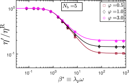
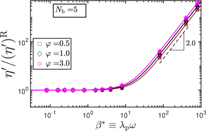
(a)	(b)
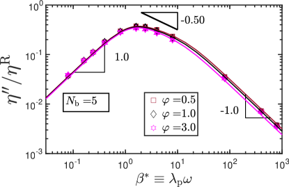
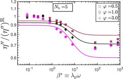
(c)	(d)

Figure 9: Plots of the real ($\eta^{\prime}$) and imaginary components ($\eta^{\prime\prime}$) of the complex viscosity, as a function of the scaled frequency, for a five-bead chain at three different values for the internal friction parameter. The lines are approximate solutions given in  Dasbach, Manke, and Williams (1992). Error bars are smaller than symbol size.

In Fig. 8 (a), the elastic component of the stress relaxation modulus for a Hookean dumbbell with internal friction is plotted as a function of dimensionless time. Both the Dasbach, Manke and Williams (DMW) approximation, and the Gaussian approximation (GA) are seen to agree with the exact BD simulation results at later times, with the deviation most strongly observed at early times. The BD simulation data is best fit by a stretched exponential of the form,

$${G^{*}_{\text{el}}(t^{*})}=\frac{G_{\text{el}}(0)}{n_{\text{p}}k_{B}T}\exp\left[(-t^{*}/\tau_{\text{k}})^{m}\right]$$ (33)

where $\tau_{\text{k}}$ and $m$ are fitting parameters, and the fitted line is used for the calculation of $\eta^{{}^{\prime\prime}}$ as described below. The approximate theories, therefore, do not capture the linear viscoelastic properties correctly, as previously noted by Hua, Schieber, and Manke (1996), who also observed that the accuracy of the approximations worsen as the IV parameter is increased.

The stretched exponential fitted to the stress relaxation modulus is subsequently used to evaluate $\eta^{\prime\prime}$

$$\eta^{{}^{\prime\prime}}(\omega)=\int_{0}^{\infty}G_{\mathrm{el}}(t)\sin(\omega\,t)dt$$ (34)

As seen from Fig. 8 (b), the imaginary component of the complex viscosity obtained from small amplitude oscillatory shear simulations, indicated by symbols, agrees well with the values obtained using Eq. (34), with a slight deviation at the lower frequencies. The scaled frequency at which the GA result deviates from BD simulation results is found to be $\beta^{*}\approx 2$. It is possible to define a dimensionless timescale, $\tau_{\text{dev}}=1/\beta^{*}=0.5$, based on this frequency. This value of the timescale is remarkably close to the time at which the GA prediction for the stress relaxation modulus is seen to deviate from the exact BD simulation data. We have therefore established the correctness of the $\eta^{\prime\prime}$ predictions obtained from small amplitude oscillatory shear flow simulations, by comparison against the values obtained from the sine-transform of the stress relaxation modulus.

In Fig. 9, the effect of the internal friction parameter on material functions in oscillatory shear flow is examined for a five-bead chain. The exact BD simulation results, indicated by symbols, are compared against the the approximate prediction given by Dasbach, Manke, and Williams (1992), shown as lines.

As seen from Fig. 9 (a), the height of the high-frequency plateau in the dynamic viscosity varies directly with the magnitude of the internal friction parameter. The low frequency, or long wavelength, response of the chain is unaffected by a variation in the internal friction parameter. In Fig. 9 (b), the dynamic viscosity normalized by its corresponding value for a Rouse chain and plotted as a function of the scaled frequency. This quantity is seen to increase as the square of the frequency, for the same reasons elaborated in connection with Fig. 6 (b).

In Fig. 9 (c), the imaginary component of the complex viscosity is scaled by the Rouse viscosity and plotted as a function of frequency. The effect of the variation in the internal friction parameter is almost negligible in the low frequency regime and is weak in the high frequency regime.

The difference between the predictions obtained using the Dasbach, Manke, and Williams (1992) approximation and the exact BD simulation results are most starkly visible in Fig. 9 (d), where the imaginary component of the complex viscosity is scaled by its corresponding value for a Rouse chain and plotted as a function of the scaled frequency. Firstly, the approximate model predicts a low-frequency plateau that is dependent on the internal friction parameter. The simulation results, however, appear to converge on a low-frequency plateau value that is almost independent of the IV parameter. Secondly, the difference between the two predictions is seen to increase with the internal friction parameter in the intermediate frequency regime, with the effect of the internal friction parameter becoming less perceptible in the high frequency regime.

Thus we see from Figs. 6 and 9 that the effect of internal friction on the real (dissipative) component of the complex viscosity is more pronounced than that on the imaginary (elastic) component.

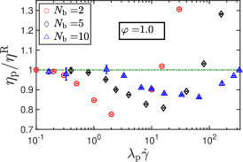
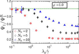
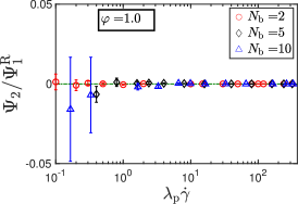
(a)	(b)	(c)
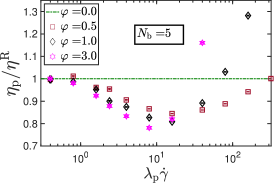
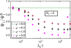
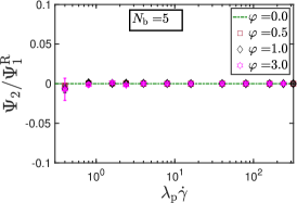
(d)	(e)	(f)

Figure 10: Steady-shear viscometric functions for bead-spring-dashpot chains with varying (a) number of beads in the chain and (b) values of the internal friction parameter. The horizontal lines in the figures indicate the material functions for a Rouse chain.

A major motivation for the inclusion of internal friction in early theoretical models for polymeric solutions Peterlin (1967); Peterlin and Reinhold (1967); Bazúa and Williams (1974) was to explain the high-frequency limiting value of the dynamic viscosity, $\eta^{\prime}(\omega\to\infty)\equiv\eta^{\prime}_{\infty}$, observed in experiments Lamb and Matheson (1964); Philippoff (1964); Massa, Schrag, and Ferry (1971). An improvement to the Rouse/Zimm models was sought since they predict that the dynamic viscosity vanishes in the limit of high frequency, in contrast with experimental observations which in most instances indicate a positive limiting value Lamb and Matheson (1964); Philippoff (1964); Massa, Schrag, and Ferry (1971). Models with internal friction, however, are able to successfully predict this plateau. There do exist systems, however, where the limiting value of the dynamic viscosity in the high frequency limit is negative Morris, Amelar, and Lodge (1988). A detailed experimental investigation of the solvent molecule and polymer segment relaxation dynamics in such systems has been conducted by Lodge and coworkers Morris, Amelar, and Lodge (1988); Lodge (1993). They conclude that such negative values of $\eta^{\prime}_{\infty}$ cannot be explained within the existing polymer kinetic theory framework. Suggested modifications to the framework comprise the inclusion of an additional term in the stress tensor expression that accounts for coupling effects between the polymer molecules and the solvent Bird (1989). It is not clear what factors determine when internal friction may be invoked to explain high frequency oscillatory shear data, and when additional physics needs to be considered. This is an important question that awaits theoretical and experimental investigation, but is beyond the scope of the present work.

III.3 Steady-shear viscometric functions

In Fig. 10, the steady-shear values of the material functions defined in Eq. (18) are scaled by the corresponding values for a Rouse chain and plotted as a function of the characteristic shear rate. Schieber has shown Schieber (1993), using the Gaussian approximation for dumbbells, that the zero-shear rate viscometric functions are unaffected by internal friction. The simulation data is found to concur with this prediction for all the three material functions. It is found that $\Psi_{2}$ is practically zero across the range of shear rates examined for all the cases.

As observed from Figs. 10 (a) and (d), there is a striking similarity in the steady-shear variation of viscosity between Rouse chains with IV, and Rouse chains with hydrodynamic interactions Zylka (1991); Prabhakar and Prakash (2006), in that there is shear-thinning followed by shear-thickening. For bead-spring-dashpot chains with a fixed number of beads, it is observed that the characteristic shear rate at which the minimum in the viscosity occurs is largely unaffected by the internal friction parameter. At shear rates larger than this critical value, the viscosity is found to increase with an increase in the IV parameter. For Rouse chains with hydrodynamic interactions, not only is the zero-shear-rate viscosity different from the free-draining case, the shear-dependence of viscosity is markedly dependent on the number of beads in the chain Zylka (1991): for $N_{\text{b}}<6$, the Rouse viscosity is lower than the Zimm viscosity, and at large shear rates, where the effect of HI weakens, the viscosity values tend towards the Rouse value, and a shear-thinning is observed, following the Newtonian plateau at low shear rates. For $N_{\text{b}}\geq 6$, however, the Rouse viscosity is greater than the Zimm viscosity, and at higher shear rates, the weakening of hydrodynamic interactions result in an upturn in the viscosity, causing it to approach the Rouse limit. An analogous explanation for the shear-thickening observed in Rouse chains with internal friction does not seem possible, since not only does the internal friction parameter result in a pronounced increase in shear thickening at high shear rates, but the viscosity is also seen to exceed the Rouse value, clearly ruling out any weakening of the internal friction effects at high shear rates.

As seen from Fig. 10 (b), the onset of shear-thinning in the first normal stress coefficient is pushed to higher shear rates, and the extent of shear-thinning reduced, with an increase in the number of beads at a fixed value of the internal friction parameter. For an internal friction parameter value of $\varphi=1.0$, and the range of shear rates examined in the present work, there does not appear to be any pronounced shear-thickening for any of the three chain lengths. BD simulations for Hookean dumbbells with internal friction by Hua and Schieber (1995) show a similar plateauing in the first normal stress coefficient, as seen in the present work. There appears to be a suggestion, but no clear evidence of shear-thickening of $\Psi_{1}$, in their work Hua and Schieber (1995).

It is anticipated that a shear-thickening in $\Psi_{1}$ would be observed at higher values of the internal friction parameter, as evidenced by Fig. 10 (e), where the effect of the internal friction parameter on the first normal stress coefficient is examined for a five-bead chain. At lower values of $\varphi$, there is no pronounced shear-thickening in $\Psi_{1}$, but a value of $\varphi=3.0$ results in the onset of a pronounced shear-thickening at $\lambda_{\text{p}}\dot{\gamma}\approx 100.0$. Furthermore, this critical shear rate for the onset of shear-thickening in $\Psi_{1}$ is about an order-of-magnitude larger than that in the case of viscosity.

It appears plausible that the shear-thickening in the viscosity and the first normal stress coefficient involves an interplay of internal friction and the number of beads in the chain.

A prevalent notion in the literature Manke and Williams (1986, 1989, 1991, 1993) is that the $\varphi\to\infty$ corresponds to the rigid-rod limit. This is supported by the following observation. The stress jump for rigid dumbbells with a Gaussian distribution of lengths is given by Hua, Schieber, and Manke (1996) $\eta_{\text{jump,rigid}}=0.4\,n_{\text{p}}k_{B}T\lambda_{H}$; while the stress jump for Hookean dumbbells with IV has the following form given by Manke and Williams Manke and Williams (1988), $\eta_{\text{jump,IV}}=0.4\left[2\varphi/(1+2\varphi)\right]n_{\text{p}}k_{B}T\lambda_{H}$. Clearly, taking the $\varphi\to\infty$ limit for Hookean spring-dashpots gives the rigid-rod dumbbell result. There is a qualitative difference in the high-shear rate behavior of rigid-rod dumbbells and bead-rod chains, in that while the viscosity of rigid dumbbells shear-thins with an asymptotic exponent of $-1/3$, that of bead-rod-chains exhibits a high shear rate plateau Petera and Muthukumar (1999); Pincus, Rodger, and Prakash (2020). In flexible chains with internal friction, however, there is no qualitative difference between the dumbbell and chain results, with a pronounced increase in the shear-thickening of viscosity as $\varphi$ is increased. Furthermore, while the first normal stress coefficient for bead-rod chains shear-thins continuously Petera and Muthukumar (1999), chains with IV exhibit a slight shear-thickening at high shear rates, as discussed previously.

A detailed comparison of the rheological properties of FENE dumbbells with IV and rigid dumbbells is given in Ref. 34 where it is concluded that a combination of finite extensibility and a high value of the internal friction parameter ($\varphi\geq 5$) is required to qualitatively mimic the steady-shear rheological response of rigid-rod models Pincus, Rodger, and Prakash (2020).

IV Conclusions

The exact set of stochastic differential equations, and a thermodynamically consistent stress tensor expression for a Rouse chain with fluctuating internal friction has been derived. The BD simulation algorithm for the solution of these equations has been validated by comparison against approximate predictions available in the literature for the stress jump, and material functions in oscillatory and steady simple shear flows have been calculated. Semi-analytical predictions Dasbach, Manke, and Williams (1992) for the dynamic viscosity are in near-quantitative agreement with the exact simulation results, with the accuracy improving with an increase in the number of beads in the chain. The difference between the predictions and the simulation results are more pronounced for the case of the imaginary component of the complex viscosity. The approximation by  Dasbach, Manke, and Williams (1992) fails to capture the frequency dependence of $\eta^{\prime\prime}$ for the dumbbell case observed in exact BD simulations and predicted by the Gaussian approximation Schieber (1993).

The approach developed by Williams and coworkers Manke and Williams (1988); Dasbach, Manke, and Williams (1992), however, is valid only in the linear viscoelastic regime, and cannot be used to obtain steady-shear viscometric predictions. The Gaussian approximation Schieber (1993) solution is only available for Hookean dumbbells with internal friction, and is unable to predict the shear-thickening in viscosity observed in exact Brownian dynamics simulations. The present work therefore extends the applicability of the Manke and Williams approach Manke and Williams (1988); Dasbach, Manke, and Williams (1992) and permits the calculation of viscometric functions in the non-linear regime, and provides an exact solution to free-draining bead-spring-dashpot chains which was previously available for only the $N_{\text{b}}=2$ case Hua and Schieber (1995).

Bead-spring-dashpot chains exhibit a non-monotonous variation in the viscosity with respect to the shear rate, with shear-thinning followed by shear-thickening. At a fixed value of the internal friction parameter, the shear-thickening effect is seen to weaken with an increase in the number of beads in the chain. Increasing the internal friction parameter at a fixed value of the number of beads in the chain leads to an increase in shear-thickening. The inclusion of internal friction results in a slight shear-thickening of the first normal stress coefficient, with the onset of thickening pushed to lower shear rates with an increase in the internal friction parameter.

The importance of hydrodynamic interactions in describing the dynamics of dilute polymer solutions is well-documented Kailasham, Chakrabarti, and Prakash (2018); Prakash (2019). However HI has not been considered in the present work, because its inclusion introduces an explicit coupling between all bead-pairs, and the procedure developed here is not applicable for the decoupling of the connector vector velocities. The solution of bead-spring-dashpot chains with hydrodynamic and excluded volume interactions is a subject for future study.

Appendix A Illustration of the decoupling methodology for a three-spring chain

We define the quantity

$$C_{k}=\dfrac{\bm{Q}_{k}\cdot\llbracket\dot{\bm{Q}}_{k}\rrbracket}{Q^{2}_{k}};\quad k=1,2,\cdots,3$$ (35)

and take a dot-product on both sides of Eq. (II) with $\llbracket\dot{\bm{Q}}_{k}\rrbracket$ to obtain the following generating equation

$$C_{k} =\left(\dfrac{\zeta}{\zeta+2K}\right)\left(\dfrac{\bm{Q}_{k}}{Q^{2}_{k}}\right)\cdot\left(\boldsymbol{\kappa}\cdot\bm{Q}_{k}\right)-{\left(\dfrac{k_{B}T}{\zeta+2K}\right)\left(\dfrac{\bm{Q}_{k}}{Q^{2}_{k}}\right)\cdot\left[-\dfrac{\partial\ln\Psi}{\partial\bm{Q}_{k-1}}+2\dfrac{\partial\ln\Psi}{\partial\bm{Q}_{k}}-\dfrac{\partial\ln\Psi}{\partial\bm{Q}_{k+1}}\right]}-\left(\dfrac{1}{\zeta+2K}\right)\left(\dfrac{\bm{Q}_{k}}{Q^{2}_{k}}\right)\cdot\Biggl{[}$$

$$-\dfrac{\partial\phi}{\partial\bm{Q}_{k-1}}+2\dfrac{\partial\phi}{\partial\bm{Q}_{k}}-\dfrac{\partial\phi}{\partial\bm{Q}_{k+1}}\Biggr{]}+\left(\dfrac{K}{\zeta+2K}\right)\left[C_{k-1}L_{k-1}\left(\dfrac{{Q}_{k-1}}{Q_{k}}\right)+C_{k+1}L_{k}\left(\dfrac{{Q}_{k+1}}{Q_{k}}\right)\right]$$ (36)

where

$$L_{k}\equiv\cos\theta_{k}=\dfrac{\boldsymbol{Q}_{k}\cdot\boldsymbol{Q}_{k+1}}{Q_{k}Q_{k+1}}$$ (37)

Eq. (A) is a coupled system of equations for the $C_{k}$, and it permits Eq. (II) to be written as

$$\llbracket\dot{\bm{Q}}_{j}\rrbracket =\boldsymbol{\kappa}\cdot\bm{Q}_{j}-\sum^{3}_{k=1}{\bm{A}}_{jk}\cdot\left(\dfrac{k_{B}T}{\zeta}\dfrac{\partial\ln\Psi}{\partial\bm{Q}_{k}}+\dfrac{1}{\zeta}\dfrac{\partial\phi}{\partial\bm{Q}_{k}}\right)-\varphi\sum^{3}_{k=1}{\bm{A}}_{jk}\cdot{\bm{Q}_{k}}C_{k}$$ (38)

The objective, then, is to obtain a decoupled expression for $C_{k}$ that would yield a decoupled expression for $\llbracket\dot{\bm{Q}}_{j}\rrbracket$ which may then readily be substituted into the equation of continuity in probability space, to obtain the governing Fokker-Planck equation for the system. The expressions for $C_{k}$ for each of the three springs are as given below.

$$C_{1} =\left(\dfrac{\zeta}{\zeta+2K}\right)\left(\dfrac{\bm{Q}_{1}}{Q^{2}_{1}}\right)\cdot\left(\boldsymbol{\kappa}\cdot\bm{Q}_{1}\right)-{\left(\dfrac{k_{B}T}{\zeta+2K}\right)\left(\dfrac{\bm{Q}_{1}}{Q^{2}_{1}}\right)\cdot\uline{\left[2\dfrac{\partial\ln\Psi}{\partial\bm{Q}_{1}}-\dfrac{\partial\ln\Psi}{\partial\bm{Q}_{2}}\right]}}$$

$$-\left(\dfrac{1}{\zeta+2K}\right)\left(\dfrac{\bm{Q}_{1}}{Q^{2}_{1}}\right)\cdot\uline{\Biggl{[}2\dfrac{\partial\phi}{\partial\bm{Q}_{1}}-\dfrac{\partial\phi}{\partial\bm{Q}_{2}}\Biggr{]}}+\left(\dfrac{K}{\zeta+2K}\right)\left[C_{2}L_{1}\left(\dfrac{{Q}_{2}}{Q_{1}}\right)\right]$$ (39)

$$C_{2} =\left(\dfrac{\zeta}{\zeta+2K}\right)\left(\dfrac{\bm{Q}_{2}}{Q^{2}_{2}}\right)\cdot\left(\boldsymbol{\kappa}\cdot\bm{Q}_{2}\right)-{\left(\dfrac{k_{B}T}{\zeta+2K}\right)\left(\dfrac{\bm{Q}_{2}}{Q^{2}_{2}}\right)\cdot\dashuline{\left[-\dfrac{\partial\ln\Psi}{\partial\bm{Q}_{1}}+2\dfrac{\partial\ln\Psi}{\partial\bm{Q}_{2}}-\dfrac{\partial\ln\Psi}{\partial\bm{Q}_{3}}\right]}}$$

$$-\left(\dfrac{1}{\zeta+2K}\right)\left(\dfrac{\bm{Q}_{2}}{Q^{2}_{2}}\right)\cdot\dashuline{\Biggl{[}-\dfrac{\partial\phi}{\partial\bm{Q}_{1}}+2\dfrac{\partial\phi}{\partial\bm{Q}_{2}}-\dfrac{\partial\phi}{\partial\bm{Q}_{3}}\Biggr{]}}+\left(\dfrac{K}{\zeta+2K}\right)\left[C_{1}L_{1}\left(\dfrac{{Q}_{1}}{Q_{2}}\right)+C_{3}L_{2}\left(\dfrac{{Q}_{3}}{Q_{2}}\right)\right]$$ (40)

$$C_{3} =\left(\dfrac{\zeta}{\zeta+2K}\right)\left(\dfrac{\bm{Q}_{3}}{Q^{2}_{3}}\right)\cdot\left(\boldsymbol{\kappa}\cdot\bm{Q}_{3}\right)-{\left(\dfrac{k_{B}T}{\zeta+2K}\right)\left(\dfrac{\bm{Q}_{3}}{Q^{2}_{3}}\right)\cdot\dotuline{\left[-\dfrac{\partial\ln\Psi}{\partial\bm{Q}_{2}}+2\dfrac{\partial\ln\Psi}{\partial\bm{Q}_{3}}\right]}}$$

$$-\left(\dfrac{1}{\zeta+2K}\right)\left(\dfrac{\bm{Q}_{3}}{Q^{2}_{3}}\right)\cdot\dotuline{\Biggl{[}-\dfrac{\partial\phi}{\partial\bm{Q}_{2}}+2\dfrac{\partial\phi}{\partial\bm{Q}_{3}}\Biggr{]}}+\left(\dfrac{K}{\zeta+2K}\right)\left[C_{2}L_{2}\left(\dfrac{{Q}_{2}}{Q_{3}}\right)\right]$$ (41)

It is clear from each pair of underlined terms in Eqs. (A) - (A) that the structure of the Brownian force and the spring force terms are identical. In the forthcoming steps, therefore, only the spring force term shall be indicated for the sake of brevity. Once a general pattern has been identified, the final expression would contain both the Brownian and the spring force terms, multiplied by the appropriate prefactors.

We note from Eq. (A) that each value of $C_{k}$ depends on both its nearest neighbors, $C_{k-1}$ and $C_{k+1}$. The terminal connector vectors, however, represent a special case since $C_{1}$ would depend only on $C_{2}$, and $C_{N}$ would depend only on $C_{N-1}$, as evident from Eqs. (A) - (A).

A.1 Forward substitution step

In this step, the expression for $C_{k}$ is substituted into that for $C_{k+1}$, iteratively from $k=1$ to $k=2$, which removes all dependence of $C_{k}$ on $C_{k-1}$, and yields an expression for $C_{k}$ solely in terms of $C_{k+1}$.

Multiplying Eq. (A) by $L_{1}(Q_{1}/Q_{2})$,

$$C_{1}L_{1}\left(\dfrac{{Q}_{1}}{Q_{2}}\right) =L_{1}\left(\dfrac{\zeta}{\zeta+2K}\right)\left(\dfrac{1}{Q_{2}}\right)\left(\dfrac{\boldsymbol{Q}_{1}}{Q_{1}}\right)\cdot\left(\boldsymbol{\kappa}\cdot\boldsymbol{Q}_{1}\right)-\left(\dfrac{1}{\zeta+2K}\right)\left(\dfrac{L_{1}}{Q_{2}}\right)\left(\dfrac{\boldsymbol{Q}_{1}}{Q_{1}}\right)\cdot\left[2\dfrac{\partial\phi}{\partial\boldsymbol{Q}_{1}}-\dfrac{\partial\phi}{\partial\boldsymbol{Q}_{2}}\right]$$ (42)

$$+\left(\dfrac{K}{\zeta+2K}\right)C_{2}L^{2}_{1}$$ (43)

and substituting into Eq. (A), we obtain

$$C_{2}=\left(\dfrac{K}{\zeta+2K}\right)C_{3}L_{2}\left(\dfrac{{Q}_{3}}{Q_{2}}\right)+\left(\dfrac{\zeta}{\zeta+2K}\right)\left(\dfrac{\boldsymbol{Q}_{2}}{Q^{2}_{2}}\right)\cdot\left(\boldsymbol{\kappa}\cdot\boldsymbol{Q}_{2}\right)+\left(\dfrac{1}{\zeta+2K}\right)\left(\dfrac{\boldsymbol{Q}_{2}}{Q^{2}_{2}}\right)\cdot\left[\dfrac{\partial\phi}{\partial\boldsymbol{Q}_{1}}\right]$$

$$-2\left(\dfrac{1}{\zeta+2K}\right)\left(\dfrac{\boldsymbol{Q}_{2}}{Q^{2}_{2}}\right)\cdot\left[\dfrac{\partial\phi}{\partial\boldsymbol{Q}_{2}}\right]+\left(\dfrac{1}{\zeta+2K}\right)\left(\dfrac{\boldsymbol{Q}_{2}}{Q^{2}_{2}}\right)\cdot\left[\dfrac{\partial\phi}{\partial\boldsymbol{Q}_{3}}\right]+\dashuline{\left(\dfrac{K}{\zeta+2K}\right)^{2}C_{2}L^{2}_{1}}$$

$$+L_{1}\left(\dfrac{K}{\zeta+2K}\right)\left(\dfrac{\zeta}{\zeta+2K}\right)\left(\dfrac{1}{Q_{2}}\right)\left(\dfrac{\boldsymbol{Q}_{1}}{Q_{1}}\right)\cdot\left(\boldsymbol{\kappa}\cdot\boldsymbol{Q}_{1}\right)$$ (44)

$$+\left(\dfrac{K}{\zeta+2K}\right)\Biggl{\{}\left(\dfrac{1}{\zeta+2K}\right)\left(\dfrac{L_{1}}{Q_{2}}\right)\left(\dfrac{\boldsymbol{Q}_{1}}{Q_{1}}\right)\cdot\left[\dfrac{\partial\phi}{\partial\boldsymbol{Q}_{2}}\right]-2\left(\dfrac{1}{\zeta+2K}\right)\left(\dfrac{L_{1}}{Q_{2}}\right)\left(\dfrac{\boldsymbol{Q}_{1}}{Q_{1}}\right)\cdot\left[\dfrac{\partial\phi}{\partial\boldsymbol{Q}_{1}}\right]\Biggr{\}}$$

Defining

$$M_{2}=\left(\dfrac{K}{\zeta+2K}\right)^{2}L^{2}_{1}$$ (45)

and grouping like terms together, the following expression for $C_{2}$ is obtained

$$C_{2} =\left(\dfrac{1}{1-M_{2}}\right)\left(\dfrac{K}{\zeta+2K}\right)C_{3}L_{2}\left(\dfrac{{Q}_{3}}{Q_{2}}\right)$$ (46)

$$+\left(\dfrac{1}{1-M_{2}}\right)\left(\dfrac{\zeta}{\zeta+2K}\right)\left(\dfrac{1}{Q_{2}}\right)\left[\left(\dfrac{\boldsymbol{Q}_{2}}{Q_{2}}\right)\cdot\left(\boldsymbol{\kappa}\cdot\boldsymbol{Q}_{2}\right)+\left(\dfrac{K}{\zeta+2K}\right)L_{1}\left(\dfrac{\boldsymbol{Q}_{1}}{Q_{1}}\right)\cdot\left(\boldsymbol{\kappa}\cdot\boldsymbol{Q}_{1}\right)\right]$$

$$+\left(\dfrac{1}{1-M_{2}}\right)\left(\dfrac{1}{\zeta+2K}\right)\left(\dfrac{\boldsymbol{Q}_{2}}{Q^{2}_{2}}\right)\cdot\left[\dfrac{\partial\phi}{\partial\boldsymbol{Q}_{3}}\right]$$

$$-\left(\dfrac{1}{1-M_{2}}\right)\left(\dfrac{1}{\zeta+2K}\right){\left(\dfrac{1}{Q_{2}}\right)\left[-\left(\dfrac{K}{\zeta+2K}\right)L_{1}\left(\dfrac{\boldsymbol{Q}_{1}}{Q_{1}}\right)+2\left(\dfrac{\boldsymbol{Q}_{2}}{Q_{2}}\right)\right]}\cdot\left(\dfrac{\partial\phi}{\partial\boldsymbol{Q}_{2}}\right)$$

$$-\left(\dfrac{1}{1-M_{2}}\right)\left(\dfrac{1}{\zeta+2K}\right){\left(\dfrac{1}{Q_{2}}\right)\left[2\left(\dfrac{K}{\zeta+2K}\right)L_{1}\left(\dfrac{\boldsymbol{Q}_{1}}{Q_{1}}\right)-\left(\dfrac{\boldsymbol{Q}_{2}}{Q_{2}}\right)\right]}\cdot\left(\dfrac{\partial\phi}{\partial\boldsymbol{Q}_{1}}\right)$$

Thus we see that the forward substitution procedure results in an expression for $C_{2}$ that depends only on $C_{3}$, which may be compared against Eq (A) in which the expression for $C_{2}$ is coupled to both $C_{1}$ and $C_{3}$.

As the next step, Eq. (46) is multiplied by $L_{2}(Q_{2}/Q_{3})$ and substituted into Eq. (A), which results in

$$C_{3}=\left(\dfrac{\zeta}{\zeta+2K}\right)\left(\dfrac{1}{Q_{3}}\right)\Biggl{[}\left(\dfrac{1}{1-M_{3}}\right)\left(\dfrac{\boldsymbol{Q}_{3}}{Q_{3}}\right)\cdot\left(\boldsymbol{\kappa}\cdot\boldsymbol{Q}_{3}\right)+\left(\dfrac{1}{1-M_{3}}\right)\left(\dfrac{1}{1-M_{2}}\right)\left(\dfrac{K}{\zeta+2K}\right)L_{2}\left(\dfrac{\boldsymbol{Q}_{2}}{Q_{2}}\right)\cdot\left(\boldsymbol{\kappa}\cdot\boldsymbol{Q}_{2}\right)$$

$$+\left(\dfrac{1}{1-M_{3}}\right)\left(\dfrac{1}{1-M_{2}}\right)\left(\dfrac{K}{\zeta+2K}\right)^{2}L_{2}L_{1}\left(\dfrac{\boldsymbol{Q}_{1}}{Q_{1}}\right)\cdot\left(\boldsymbol{\kappa}\cdot\boldsymbol{Q}_{1}\right)\Biggr{]}$$

$$-\left(\dfrac{1}{\zeta+2K}\right)\left(\dfrac{1}{Q_{3}}\right)\Biggl{[}-\left(\dfrac{1}{1-M_{3}}\right)\left(\dfrac{1}{1-M_{2}}\right)\left(\dfrac{K}{\zeta+2K}\right)L_{2}\left(\dfrac{\boldsymbol{Q}_{2}}{Q_{2}}\right)+2\left(\dfrac{1}{1-M_{3}}\right)\left(\dfrac{\boldsymbol{Q}_{3}}{Q_{3}}\right)\Biggr{]}\cdot\left(\dfrac{\partial\phi}{\partial\boldsymbol{Q}_{3}}\right)$$

$$-\left(\dfrac{1}{\zeta+2K}\right)\left(\dfrac{1}{Q_{3}}\right)\Biggl{[}-\left(\dfrac{1}{1-M_{3}}\right)\left(\dfrac{1}{1-M_{2}}\right)\left(\dfrac{K}{\zeta+2K}\right)^{2}L_{2}L_{1}\left(\dfrac{\boldsymbol{Q}_{1}}{Q_{1}}\right)$$

$$\qquad\qquad+2\left(\dfrac{1}{1-M_{3}}\right)\left(\dfrac{1}{1-M_{2}}\right)\left(\dfrac{K}{\zeta+2K}\right)L_{2}\left(\dfrac{\boldsymbol{Q}_{2}}{Q_{2}}\right)-\left(\dfrac{\boldsymbol{Q}_{3}}{Q_{3}}\right)\Biggr{]}\cdot\left(\dfrac{\partial\phi}{\partial\boldsymbol{Q}_{2}}\right)$$

$$-\left(\dfrac{1}{\zeta+2K}\right)\left(\dfrac{1}{Q_{3}}\right)\Biggl{[}2\left(\dfrac{K}{\zeta+2K}\right)^{2}\left(\dfrac{1}{1-M_{3}}\right)\left(\dfrac{1}{1-M_{2}}\right)L_{2}L_{1}\left(\dfrac{\boldsymbol{Q}_{1}}{Q_{1}}\right)$$ (47)

$$\qquad\qquad\qquad\qquad-\left(\dfrac{K}{\zeta+2K}\right)\left(\dfrac{1}{1-M_{3}}\right)\left(\dfrac{1}{1-M_{2}}\right)L_{2}\left(\dfrac{\boldsymbol{Q}_{2}}{Q_{2}}\right)\Biggr{]}\cdot\left(\dfrac{\partial\phi}{\partial\boldsymbol{Q}_{1}}\right)$$

where

$$M_{3}=\left(\dfrac{K}{\zeta+2K}\right)^{2}\left(\dfrac{1}{1-M_{2}}\right)L^{2}_{2}$$ (48)

Since $C_{3}$ is the terminal connector vector in a three-spring chain, one obtains a completely decoupled expression for it by the application of the forward substitution procedure.

A.2 Backward substitution step

In this step, the expression for $C_{k}$ is substituted into that for $C_{k-1}$, iteratively from $k=3$ to $k=2$. Multiplying Eq. (A) by $L_{2}(Q_{3}/Q_{2})$,

$$C_{3}L_{2}\left(\dfrac{Q_{3}}{Q_{2}}\right)=\left(\dfrac{\zeta}{\zeta+2K}\right)\left(\dfrac{L_{2}}{Q_{2}}\right)\left(\dfrac{\boldsymbol{Q}_{3}}{Q_{3}}\right)\cdot\left(\boldsymbol{\kappa}\cdot\boldsymbol{Q}_{3}\right)+\left(\dfrac{K}{\zeta+2K}\right)\left[{C_{2}L^{2}_{2}}\right]$$ (49)

$$+\left(\dfrac{1}{\zeta+2K}\right)\left(\dfrac{L_{2}}{Q_{2}}\right)\left(\dfrac{\boldsymbol{Q}_{3}}{Q_{3}}\right)\cdot\left(\dfrac{\partial\phi}{\partial\boldsymbol{Q}_{2}}\right)-2\left(\dfrac{1}{\zeta+2K}\right)\left(\dfrac{L_{2}}{Q_{2}}\right)\left(\dfrac{\boldsymbol{Q}_{3}}{Q_{3}}\right)\cdot\left(\dfrac{\partial\phi}{\partial\boldsymbol{Q}_{3}}\right)$$

and substituting into Eq. (A), we obtain

$$C_{2}=\left(\dfrac{K}{\zeta+2K}\right)C_{1}L_{1}\left(\dfrac{{Q}_{1}}{Q_{2}}\right)+\left(\dfrac{\zeta}{\zeta+2K}\right)\left(\dfrac{\boldsymbol{Q}_{2}}{Q^{2}_{2}}\right)\cdot\left(\boldsymbol{\kappa}\cdot\boldsymbol{Q}_{2}\right)+\dashuline{\left(\dfrac{K}{\zeta+2K}\right)^{2}C_{2}L^{2}_{2}}$$

$$+\left(\dfrac{1}{\zeta+2K}\right)\left(\dfrac{1}{Q_{2}}\right)\left(\dfrac{\boldsymbol{Q}_{2}}{Q_{2}}\right)\cdot\left(\dfrac{\partial\phi}{\partial\boldsymbol{Q}_{1}}\right)-2\left(\dfrac{1}{\zeta+2K}\right)\left(\dfrac{1}{Q_{2}}\right)\left(\dfrac{\boldsymbol{Q}_{2}}{Q_{2}}\right)\cdot\left(\dfrac{\partial\phi}{\partial\boldsymbol{Q}_{2}}\right)$$

$$+\left(\dfrac{1}{\zeta+2K}\right)\left(\dfrac{1}{Q_{2}}\right)\left(\dfrac{\boldsymbol{Q}_{2}}{Q_{2}}\right)\cdot\left(\dfrac{\partial\phi}{\partial\boldsymbol{Q}_{3}}\right)+\left(\dfrac{\zeta}{\zeta+2K}\right)\left(\dfrac{K}{\zeta+2K}\right)L_{2}\left(\dfrac{1}{Q_{2}}\right)\left(\dfrac{\boldsymbol{Q}_{3}}{Q_{3}}\right)\cdot\left(\boldsymbol{\kappa}\cdot\boldsymbol{Q}_{3}\right)$$ (50)

$$+\left(\dfrac{1}{\zeta+2K}\right)\left(\dfrac{K}{\zeta+2K}\right)\left(\dfrac{1}{Q_{2}}\right)L_{2}\left(\dfrac{\boldsymbol{Q}_{3}}{Q_{3}}\right)\cdot\left(\dfrac{\partial\phi}{\partial\boldsymbol{Q}_{2}}\right)-2\left(\dfrac{1}{\zeta+2K}\right)\left(\dfrac{K}{\zeta+2K}\right)\left(\dfrac{1}{Q_{2}}\right)L_{2}\left(\dfrac{\boldsymbol{Q}_{3}}{Q_{3}}\right)\cdot\left(\dfrac{\partial\phi}{\partial\boldsymbol{Q}_{3}}\right)$$

Defining

$$P_{2}={\left(\dfrac{K}{\zeta+2K}\right)^{2}L^{2}_{2}}$$ (51)

and grouping like terms together, we have

$$C_{2}=\left(\dfrac{1}{1-P_{2}}\right)\left(\dfrac{K}{\zeta+2K}\right)C_{1}L_{1}\left(\dfrac{{Q}_{1}}{Q_{2}}\right)+\left(\dfrac{\zeta}{\zeta+2K}\right)\left(\dfrac{1}{Q_{2}}\right)\Biggl{[}\left(\dfrac{1}{1-P_{2}}\right)\left(\dfrac{\boldsymbol{Q}_{2}}{Q_{2}}\right)\cdot\left(\boldsymbol{\kappa}\cdot\boldsymbol{Q}_{2}\right)$$

$$+\left(\dfrac{K}{\zeta+2K}\right)\left(\dfrac{1}{1-P_{2}}\right)L_{2}\left(\dfrac{\boldsymbol{Q}_{3}}{Q_{3}}\right)\cdot\left(\boldsymbol{\kappa}\cdot\boldsymbol{Q}_{3}\right)\Biggr{]}+\left(\dfrac{1}{\zeta+2K}\right)\left(\dfrac{1}{1-P_{2}}\right)\left(\dfrac{1}{Q_{2}}\right)\left(\dfrac{\boldsymbol{Q}_{2}}{Q_{2}}\right)\cdot\left(\dfrac{\partial\phi}{\partial\boldsymbol{Q}_{1}}\right)$$

$$-\left(\dfrac{1}{\zeta+2K}\right)\left(\dfrac{1}{Q_{2}}\right)\Biggl{[}-\left(\dfrac{1}{1-P_{2}}\right)\left(\dfrac{K}{\zeta+2K}\right)L_{2}\left(\dfrac{\boldsymbol{Q}_{3}}{Q_{3}}\right)+2\left(\dfrac{1}{1-P_{2}}\right)\left(\dfrac{\boldsymbol{Q}_{2}}{Q_{2}}\right)\Biggr{]}\cdot\left(\dfrac{\partial\phi}{\partial\boldsymbol{Q}_{2}}\right)$$

$$-\left(\dfrac{1}{\zeta+2K}\right)\left(\dfrac{1}{Q_{2}}\right)\Biggl{[}2\left(\dfrac{1}{1-P_{2}}\right)\left(\dfrac{K}{\zeta+2K}\right)L_{2}\left(\dfrac{\boldsymbol{Q}_{3}}{Q_{3}}\right)-\left(\dfrac{1}{1-P_{2}}\right)\left(\dfrac{\boldsymbol{Q}_{2}}{Q_{2}}\right)\Biggr{]}\cdot\left(\dfrac{\partial\phi}{\partial\boldsymbol{Q}_{3}}\right)$$ (52)

Thus we see that the backward substitution procedure results in an expression for $C_{2}$ that depends only on $C_{1}$, which may be compared against Eq (A) in which the expression for $C_{2}$ is coupled to both $C_{1}$ and $C_{3}$. Multiplying Eq. (A.2) by $L_{1}(Q_{2}/Q_{1})$,

$$C_{2}L_{1}\left(\dfrac{Q_{2}}{Q_{1}}\right)=\left(\dfrac{1}{1-P_{2}}\right)\left(\dfrac{K}{\zeta+2K}\right)C_{1}L^{2}_{1}$$ (53)

$$+\left(\dfrac{\zeta}{\zeta+2K}\right)\left(\dfrac{1}{Q_{1}}\right)\Biggl{[}\left(\dfrac{1}{1-P_{2}}\right)L_{1}\left(\dfrac{\boldsymbol{Q}_{2}}{Q_{2}}\right)\cdot\left(\boldsymbol{\kappa}\cdot\boldsymbol{Q}_{2}\right)+\left(\dfrac{K}{\zeta+2K}\right)\left(\dfrac{1}{1-P_{2}}\right)L_{1}L_{2}\left(\dfrac{\boldsymbol{Q}_{3}}{Q_{3}}\right)\cdot\left(\boldsymbol{\kappa}\cdot\boldsymbol{Q}_{3}\right)\Biggr{]}$$

$$+\left(\dfrac{1}{\zeta+2K}\right)\left(\dfrac{1}{1-P_{2}}\right)L_{1}\left(\dfrac{1}{Q_{1}}\right)\left(\dfrac{\boldsymbol{Q}_{2}}{Q_{2}}\right)\cdot\left(\dfrac{\partial\phi}{\partial\boldsymbol{Q}_{1}}\right)$$

$$-\left(\dfrac{1}{\zeta+2K}\right)\left(\dfrac{1}{Q_{1}}\right)\Biggl{[}-\left(\dfrac{1}{1-P_{2}}\right)\left(\dfrac{K}{\zeta+2K}\right)L_{1}L_{2}\left(\dfrac{\boldsymbol{Q}_{3}}{Q_{3}}\right)+2\left(\dfrac{1}{1-P_{2}}\right)L_{1}\left(\dfrac{\boldsymbol{Q}_{2}}{Q_{2}}\right)\Biggr{]}\cdot\left(\dfrac{\partial\phi}{\partial\boldsymbol{Q}_{2}}\right)$$

$$-\left(\dfrac{1}{\zeta+2K}\right)\left(\dfrac{1}{Q_{1}}\right)\Biggl{[}2\left(\dfrac{1}{1-P_{2}}\right)\left(\dfrac{K}{\zeta+2K}\right)L_{1}L_{2}\left(\dfrac{\boldsymbol{Q}_{3}}{Q_{3}}\right)-\left(\dfrac{1}{1-P_{N-1}}\right)L_{1}\left(\dfrac{\boldsymbol{Q}_{2}}{Q_{2}}\right)\Biggr{]}\cdot\left(\dfrac{\partial\phi}{\partial\boldsymbol{Q}_{3}}\right)$$

and substituting into Eq. (A), we obtain We thus have the following final expression for $C_{N-2}$,

$$C_{1}=\left(\dfrac{\zeta}{\zeta+2K}\right)\left(\dfrac{1}{Q_{1}}\right)\Biggl{[}\left(\dfrac{1}{1-P_{1}}\right)\left(\dfrac{\boldsymbol{Q}_{1}}{Q_{1}}\right)\cdot\left(\boldsymbol{\kappa}\cdot\boldsymbol{Q}_{1}\right)+\left(\dfrac{K}{\zeta+2K}\right)\left(\dfrac{1}{1-P_{1}}\right)\left(\dfrac{1}{1-P_{2}}\right)L_{1}\left(\dfrac{\boldsymbol{Q}_{2}}{Q_{2}}\right)\cdot\left(\boldsymbol{\kappa}\cdot\boldsymbol{Q}_{2}\right)$$

$$+\left(\dfrac{K}{\zeta+2K}\right)^{2}\left(\dfrac{1}{1-P_{1}}\right)\left(\dfrac{1}{1-P_{2}}\right)L_{1}L_{2}\left(\dfrac{\boldsymbol{Q}_{3}}{Q_{3}}\right)\cdot\left(\boldsymbol{\kappa}\cdot\boldsymbol{Q}_{3}\right)\Biggr{]}$$

$$-\left(\dfrac{1}{\zeta+2K}\right)\left(\dfrac{1}{Q_{1}}\right)\Biggl{[}-\left(\dfrac{K}{\zeta+2K}\right)\left(\dfrac{1}{1-P_{1}}\right)\left(\dfrac{1}{1-P_{2}}\right)L_{1}\left(\dfrac{\boldsymbol{Q}_{2}}{Q_{2}}\right)+2\left(\dfrac{1}{1-P_{1}}\right)\left(\dfrac{\boldsymbol{Q}_{1}}{Q_{1}}\right)\Biggr{]}\cdot\left(\dfrac{\partial\phi}{\partial\boldsymbol{Q}_{1}}\right)$$

$$-\left(\dfrac{1}{\zeta+2K}\right)\left(\dfrac{1}{Q_{1}}\right)\Biggl{[}-\left(\dfrac{1}{1-P_{1}}\right)\left(\dfrac{1}{1-P_{2}}\right)\left(\dfrac{K}{\zeta+2K}\right)^{2}L_{1}L_{2}\left(\dfrac{\boldsymbol{Q}_{3}}{Q_{3}}\right)$$

$$+2\left(\dfrac{1}{1-P_{1}}\right)\left(\dfrac{1}{1-P_{2}}\right)\left(\dfrac{K}{\zeta+2K}\right)L_{1}\left(\dfrac{\boldsymbol{Q}_{2}}{Q_{2}}\right)-\left(\dfrac{1}{1-P_{1}}\right)\left(\dfrac{\boldsymbol{Q}_{1}}{Q_{1}}\right)\Biggr{]}\cdot\left(\dfrac{\partial\phi}{\partial\boldsymbol{Q}_{2}}\right)$$

$$-\left(\dfrac{1}{\zeta+2K}\right)\left(\dfrac{1}{Q_{1}}\right)\Biggl{[}2\left(\dfrac{1}{1-P_{1}}\right)\left(\dfrac{1}{1-P_{2}}\right)\left(\dfrac{K}{\zeta+2K}\right)^{2}L_{1}L_{2}\left(\dfrac{\boldsymbol{Q}_{3}}{Q_{3}}\right)$$

$$-\left(\dfrac{1}{1-P_{1}}\right)\left(\dfrac{1}{1-P_{2}}\right)\left(\dfrac{K}{\zeta+2K}\right)L_{1}\left(\dfrac{\boldsymbol{Q}_{2}}{Q_{2}}\right)\Biggr{]}\cdot\left(\dfrac{\partial\phi}{\partial\boldsymbol{Q}_{3}}\right)$$ (54)

where

$$P_{1}=\left(\dfrac{1}{1-P_{2}}\right)\left(\dfrac{K}{\zeta+2K}\right)^{2}L^{2}_{1}$$ (55)

A.3 Combining output from forward and backward substitution steps to obtain decoupled expression

Since $C_{1}$ and $C_{3}$ represent the terminal connector vectors in a three-spring chain, their decoupled expressions were obtained from a single iteration of the backward and forward steps, respectively. The decoupled expression for connector vectors not at the chain end [$C_{2}$ in the present case] is obtained by combining the output from the forward and backward substitution steps. For instance, the decoupled expression for $C_{2}$ may be obtained by substituting Eq. (49) into Eq. (46). From the pattern observed in these decoupled expressions, a general expression for the decoupled $C_{k}$ may be written, by induction, to be

$$\begin{split}&C_{k}=\left(\dfrac{\zeta}{\zeta+2K}\right)\left(\dfrac{1}{Q_{k}}\right)\sum_{l=1}^{N}{\boldsymbol{\Lambda}}^{(k)}_{l}\cdot\left(\boldsymbol{\kappa}\cdot\boldsymbol{Q}_{l}\right)-\left(\dfrac{\zeta}{\zeta+2K}\right)\left(\dfrac{1}{Q_{k}}\right)\Biggl{[}\left(\dfrac{k_{B}T}{\zeta}\right)\sum_{l=1}^{N}{\boldsymbol{J}}^{(k)}_{l}\cdot\left(\dfrac{\partial\ln\Psi}{\partial\boldsymbol{Q}_{l}}\right)\\[5.0pt] &+\left(\dfrac{1}{\zeta}\right)\sum_{l=1}^{N}{\boldsymbol{J}}^{(k)}_{l}\cdot\left(\dfrac{\partial\phi}{\partial\boldsymbol{Q}_{l}}\right)\Biggr{]}\end{split}$$ (56)

The definitions of the vectors $\boldsymbol{\Lambda}^{(k)}_{l}$ and $\boldsymbol{J}^{(k)}_{l}$ for the $k=1$ and $k=3$ cases are readily apparent from comparison against Eqs. (A.1) and (A.2), respectively. We provide below the definitions for the $k=2$ case

$$\boldsymbol{\Lambda}^{(2)}_{1}=\left(\dfrac{1}{1-M_{2}-P_{2}}\right)\left(\dfrac{K}{\zeta+2K}\right)L_{1}\left(\dfrac{\boldsymbol{Q}_{1}}{Q_{1}}\right)$$ (57)

$$\boldsymbol{\Lambda}^{(2)}_{2}=\left(\dfrac{1}{1-M_{2}-P_{2}}\right)\left(\dfrac{\boldsymbol{Q}_{2}}{Q_{2}}\right)$$ (58)

$$\boldsymbol{\Lambda}^{(2)}_{3}=\left(\dfrac{1}{1-M_{2}-P_{2}}\right)\left(\dfrac{K}{\zeta+2K}\right)L_{2}\left(\dfrac{\boldsymbol{Q}_{3}}{Q_{3}}\right)$$ (59)

$$\boldsymbol{J}^{(2)}_{1}=\left(\dfrac{1}{1-M_{2}-P_{2}}\right)\Biggl{[}2\left(\dfrac{K}{\zeta+2K}\right)L_{1}\left(\dfrac{\boldsymbol{Q}_{1}}{Q_{1}}\right)-\left(\dfrac{\bm{Q}_{2}}{Q_{2}}\right)\Biggr{]}$$ (60)

$$\boldsymbol{J}^{(2)}_{2}=\left(\dfrac{1}{1-M_{2}-P_{2}}\right)\Biggl{[}2\left(\dfrac{\boldsymbol{Q}_{2}}{Q_{2}}\right)-\left(\dfrac{K}{\zeta+2K}\right)L_{1}\left(\dfrac{\boldsymbol{Q}_{1}}{Q_{1}}\right)-\left(\dfrac{K}{\zeta+2K}\right)L_{2}\left(\dfrac{\boldsymbol{Q}_{3}}{Q_{3}}\right)\Biggr{]}$$ (61)

$$\boldsymbol{J}^{(2)}_{3}=\left(\dfrac{1}{1-M_{2}-P_{2}}\right)\Biggl{[}2\left(\dfrac{K}{\zeta+2K}\right)L_{2}\left(\dfrac{\boldsymbol{Q}_{3}}{Q_{3}}\right)-\left(\dfrac{\boldsymbol{Q}_{2}}{Q_{2}}\right)\Biggr{]}$$ (62)

While the expressions for the vectors $\boldsymbol{\Lambda}^{(k)}_{l}$ and $\boldsymbol{J}^{(k)}_{l}$ have been calculated in this Appendix in a brute-force manner, to illustrate the working of the decoupling machinery, computer simulation of bead-spring-dashpot chains of arbitrary length ($N$) would require an algorithmic procedure for the construction of these terms, which has been described in detail in Sec. SII of the Supplementary Material. Substituting Eq. (56) into Eq. (38) and simplifying results in the following general equation for the decoupled connector vector velocity

$$\begin{split}\llbracket\dot{\boldsymbol{Q}}_{j}\rrbracket&=\boldsymbol{\kappa}\cdot\boldsymbol{Q}_{j}-\sum^{N}_{k=1}{\boldsymbol{A}}_{jk}\cdot\left(\dfrac{k_{B}T}{\zeta}\dfrac{\partial\ln\Psi}{\partial\boldsymbol{Q}_{k}}+\dfrac{1}{\zeta}\dfrac{\partial\phi}{\partial\boldsymbol{Q}_{k}}\right)-\left(\dfrac{\varphi}{1+2\varphi}\right)\sum^{N}_{k,l=1}{\boldsymbol{A}}_{jk}\cdot\boldsymbol{\alpha}_{kl}\cdot\left(\boldsymbol{\kappa}\cdot\boldsymbol{Q}_{l}\right)\\[5.0pt] &+\left(\dfrac{k_{B}T}{\zeta}\right)\left(\dfrac{\varphi}{1+2\varphi}\right)\sum^{N}_{k,l=1}{\boldsymbol{A}}_{jk}\cdot{\boldsymbol{\mu}_{kl}}\cdot\left(\dfrac{\partial\ln\Psi}{\partial\boldsymbol{Q}_{l}}\right)+\left(\dfrac{1}{\zeta}\right)\left(\dfrac{\varphi}{1+2\varphi}\right)\sum^{N}_{k,l=1}{\boldsymbol{A}}_{jk}\cdot\boldsymbol{\mu}_{kl}\cdot\left(\dfrac{\partial\phi}{\partial\boldsymbol{Q}_{l}}\right)\end{split}$$ (63)

where the tensors

$$\begin{split}\boldsymbol{\alpha}_{kl}&=\left(\dfrac{\boldsymbol{Q}_{k}}{Q_{k}}\right){\boldsymbol{\Lambda}}^{(k)}_{l}=\chi^{(k)}_{l}\left(\dfrac{\boldsymbol{Q}_{k}\boldsymbol{Q}_{l}}{Q_{k}Q_{l}}\right),\\[5.0pt] \boldsymbol{\mu}_{kl}&={\left(\dfrac{\boldsymbol{Q}_{k}}{Q_{k}}\right){\boldsymbol{J}}^{(k)}_{l}}\end{split}$$ (64)

are used in the evaluation of the stress tensor expression as seen from Eq. (16). Additionally, the tensors $\bm{U}_{jk}$ and $\bm{V}_{jk}$ are defined as follows

$$\begin{split}\boldsymbol{U}_{jk}&=\sum_{l=1}^{N}\boldsymbol{A}_{jl}\cdot\boldsymbol{\alpha}_{lk};\quad\boldsymbol{V}_{jk}=\sum_{l=1}^{N}\boldsymbol{A}_{jl}\cdot\boldsymbol{\mu}_{lk}\end{split}$$ (65)

and feature in the governing Fokker-Planck equation given by Eq. (9). The dimensionless Fokker-Planck equation for the three-spring chain is written in terms of collective coordinates (introduced in Eq. (10)) as

$$\dfrac{\partial\psi^{*}}{\partial t^{*}} =-\dfrac{\partial}{\partial\widetilde{\bm{Q}}^{*}}\cdot\Biggl{\{}\Biggl{[}\bm{\mathcal{K}}^{*}\cdot\widetilde{\bm{Q}}^{*}-\left(\dfrac{\varphi}{1+2\varphi}\right){\bm{\mathcal{U}}}\cdot\left(\bm{\mathcal{K}}^{*}\cdot\widetilde{\bm{Q}}^{*}\right)-\dfrac{1}{4}\bm{\mathcal{D}}(\varphi)\cdot\widetilde{\bm{F}}^{*\text{s}}-\dfrac{1}{4}\left(\dfrac{\varphi}{1+2\varphi}\right)\widetilde{\bm{v}}^{*}\Biggr{]}\psi^{*}\Biggr{\}}$$

$$+\dfrac{1}{4}\dfrac{\partial}{\partial\widetilde{\bm{Q}}^{*}}\dfrac{\partial}{\partial\widetilde{\bm{Q}}^{*}}:\left[\bm{\mathcal{D}}(\varphi)\psi^{*}\right]$$

where $\bm{\mathcal{D}}(\varphi)$ is an internal friction-dependent $3\times 3$ block matrix with the following structure

$$\bm{\mathcal{D}}(\varphi)=\begin{pmatrix}\widehat{\boldsymbol{A}}_{11}&\widehat{\boldsymbol{A}}_{12}&{\widehat{\boldsymbol{A}}_{13}}\\[5.0pt] {\widehat{\boldsymbol{A}}_{21}}&{\widehat{\boldsymbol{A}}_{22}}&{\widehat{\boldsymbol{A}}_{23}}\\[5.0pt] {\widehat{\boldsymbol{A}}_{31}}&{\widehat{\boldsymbol{A}}_{32}}&{\widehat{\boldsymbol{A}}_{33}}\end{pmatrix};\quad\widehat{\boldsymbol{A}}_{jk}=\boldsymbol{A}_{jk}-\dfrac{\varphi}{1+2\varphi}\boldsymbol{V}_{jk}$$ (66)

References

- Kuhn and Kuhn (1945) W. Kuhn and H. Kuhn, Helv. Chim. Acta 28, 1533 (1945).
- Booij and van Wiechen (1970) H. C. Booij and P. H. van Wiechen, J. Chem. Phys. 52, 5056 (1970).
- de Gennes (1979) P.-G. de Gennes, Scaling Concepts in Polymer Physics (Cornell University Press, Ithaca, 1979).
- Manke and Williams (1985) C. W. Manke and M. C. Williams, Macromolecules 18, 2045 (1985).
- Manke and Williams (1988) C. W. Manke and M. C. Williams, J. Rheol. 31, 495 (1988).
- Dasbach, Manke, and Williams (1992) T. P. Dasbach, C. W. Manke, and M. C. Williams, J. Phys. Chem. 96, 4118 (1992).
- Gerhardt and Manke (1994) L. J. Gerhardt and C. W. Manke, J. Rheol. 38, 1227 (1994).
- Murayama, Wada, and Sano (2007) Y. Murayama, H. Wada, and M. Sano, Eur. Phys. Lett. 79, 58001 (2007).
- Alexander-Katz, Wada, and Netz (2009) A. Alexander-Katz, H. Wada, and R. R. Netz, Phys. Rev. Lett. 103, 028102 (2009).
- Schulz, Miettinen, and Netz (2015) J. C. F. Schulz, M. S. Miettinen, and R. R. Netz, J. Phys. Chem. B 119, 4565 (2015).
- Kailasham, Chakrabarti, and Prakash (2020) R. Kailasham, R. Chakrabarti, and J. R. Prakash, Phys. Rev. Res. 2, 013331 (2020).
- Vincenzi (2021) D. Vincenzi, Soft Matter , (2021).
- Arbe et al. (2001) A. Arbe, M. Monkenbusch, J. Stellbrink, D. Richter, B. Farago, K. Almdal, and R. Faust, Macromolecules 34, 1281 (2001).
- Poirier and Marko (2002) M. G. Poirier and J. F. Marko, Phys. Rev. Lett. 88, 4 (2002).
- Khatri et al. (2007) B. S. Khatri, M. Kawakami, K. Byrne, D. A. Smith, and T. C. B. McLeish, Biophys. J. 92, 1825 (2007).
- Qiu and Hagen (2004) L. Qiu and S. J. Hagen, J. Am. Chem. Soc. 126, 3398 (2004).
- Soranno et al. (2012) A. Soranno, B. Buchli, D. Nettels, R. R. Cheng, S. Müller-Späth, S. H. Pfeil, A. Hoffmann, E. A. Lipman, D. E. Makarov, and B. Schuler, Proc. Natl. Acad. Sci. U.S.A. 109, 17800 (2012).
- Samanta and Chakrabarti (2013) N. Samanta and R. Chakrabarti, Chem. Phys. Lett. 582, 71 (2013).
- Samanta, Ghosh, and Chakrabarti (2014) N. Samanta, J. Ghosh, and R. Chakrabarti, AIP Adv. 4, 067102 (2014).
- Samanta and Chakrabarti (2016) N. Samanta and R. Chakrabarti, Physica A 450, 165 (2016).
- Sashi, Ramakrishna, and Bhuyan (2016) P. Sashi, D. Ramakrishna, and A. K. Bhuyan, Biochemistry 55, 4595 (2016).
- Soranno et al. (2017) A. Soranno, A. Holla, F. Dingfelder, D. Nettels, D. E. Makarov, and B. Schuler, Proc. Natl. Acad. Sci. U.S.A. 114, E1833 (2017).
- Das and Makarov (2018) A. Das and D. E. Makarov, J. Phys. Chem. B 122, 9049 (2018).
- Mondal, Adhikari, and Sharma (2020) D. Mondal, R. Adhikari, and P. Sharma, Sci. Adv. 6, eabb0503 (2020).
- Subramanian et al. (2020) S. Subramanian, H. Golla, K. Divakar, A. Kannan, D. De Sancho, and A. N. Naganathan, J. Phys. Chem. B 124, 8973 (2020).
- Liang and Mackay (1993) C.-H. Liang and M. E. Mackay, J. Rheol. 37, 149 (1993).
- Orr and Sridhar (1996) N. V. Orr and T. Sridhar, J. Non-Newtonian Fluid Mech. 67, 77 (1996).
- Bird et al. (1987) R. B. Bird, C. F. Curtiss, R. C. Armstrong, and O. Hassager, Dynamics of Polymeric Liquids - Volume 2 : Kinetic Theory (John Wiley and Sons, New York, 1987).
- Öttinger (1996) H. C. Öttinger, Stochastic Processes in Polymeric Fluids (Springer, Berlin, 1996).
- Ravi Prakash (1999) J. Ravi Prakash, “The kinetic theory of dilute solutions of flexible polymers: Hydrodynamic interaction,” in Advances in the Flow and Rheology of Non-Newtonian Fluids, Rheology Series, Vol. 8, edited by D. Siginer, D. De Kee, and R. Chhabra (Elsevier, Netherlands, 1999) pp. 467–517, 1st ed.
- Schieber and Öttinger (1994) J. D. Schieber and H. C. Öttinger, J. Rheol. 38, 1909 (1994).
- Schieber (1993) J. D. Schieber, J. Rheol. 37, 1003 (1993).
- Wedgewood (1993) L. E. Wedgewood, Rheologica Acta 32, 405 (1993).
- Kailasham, Chakrabarti, and Prakash (2018) R. Kailasham, R. Chakrabarti, and J. R. Prakash, J. Chem. Phys. 149, 094903 (2018).
- Ansari et al. (1992) A. Ansari, C. M. Jones, E. R. Henry, J. Hofrichter, and W. A. Eaton, Science 256, 1796 (1992).
- Schulz et al. (2012) J. C. F. Schulz, L. Schmidt, R. B. Best, J. Dzubiella, and R. R. Netz, J. Am. Chem. Soc. 134, 6273 (2012).
- Ameseder et al. (2018) F. Ameseder, A. Radulescu, O. Holderer, P. Falus, D. Richter, and A. M. Stadler, J. Phys. Chem. Lett. 9, 2469 (2018).
- Khatri and McLeish (2007) B. S. Khatri and T. C. B. McLeish, Macromolecules 40, 6770 (2007).
- Kailasham, Chakrabarti, and Prakash (2021) R. Kailasham, R. Chakrabarti, and J. R. Prakash, “How important are fluctuations in the treatment of internal friction in polymers?” (2021), arXiv:2103.07140 [cond-mat.soft] .
- Bazúa and Williams (1974) E. R. Bazúa and M. C. Williams, J. Polym. Sci. Polym. Phys. Ed. 12, 825 (1974).
- Manke and Williams (1989) C. W. Manke and M. C. Williams, J. Rheol. 33, 949 (1989).
- Cerf (1957) R. Cerf, J. Polym. Sci. 23, 125 (1957).
- R. Cerf (1969) R. Cerf, J. Chim. Phys. 66, 479 (1969).
- Peterlin (1967) A. Peterlin, J. Polym. Sci. A-2 Polym. Phys. 5, 179 (1967).
- Hua and Schieber (1995) C. C. Hua and J. D. Schieber, J. Non-Newtonian Fluid Mech. 56, 307 (1995).