Quantum transport in non-Markovian dynamically-disordered photonic lattices

Abstract

We theoretically show that the dynamics of a driven quantum harmonic oscillator subject to non-dissipative noise is formally equivalent to the single-particle dynamics propagating through an experimentally feasible dynamically-disordered photonic network. Using this correspondence, we find that noise assisted energy transport occurs in this network and, if the noise is Markovian or delta-correlated, we can obtain an analytical solution for the maximum amount of transferred energy between all network’s sites at a fixed propagation distance. Beyond the Markovian limit, we further consider two different types of non-Markovian noise and show that it is possible to have efficient energy transport for larger values of the dephasing rate.

I Introduction

From a practical point of view, decoherence (the irreversible loss of quantum coherence) is a multifaceted process which presents advantages and disadvantages depending on the particular circumstances and application. For instance, from the perspective of perfect state transport, decoherence is the opponent to overcome since it may destroy the states way before they can be conveyed Bose (2003). On the contrary, to perform highly-efficient energy transport protocols, decoherence has been found to be the best allied Plenio and Huelga (2008); Rebentrost et al. (2009). Thus, a good understanding of the impact of decoherence on energy transport and energy conversion in the quantum and classical regimes is essential to design functional technologies based on hybrid systems Kurizki et al. (2015), ranging from quantum information processing tasks to quantum thermodynamics applications  Scully et al. (2011); Pezzutto et al. (2019); Román-Ancheyta et al. (2020); Salado-Mejía et al. (2021).

In optics, one can use integrated photonic devices, e.g., based on direct laser-writing coupled waveguides lattices Szameit and Nolte (2010); Gräfe et al. (2016), to study coherent energy transport Perez-Leija et al. (2013); Biggerstaff et al. (2016); Bossé and Vinet (2017), which is an important ingredient in the development of integrated photonic quantum technologies O’Brien et al. (2009); Wang et al. (2020). Such devices constitute a well-established, popular and relatively low-cost platform among experimentalists due to their practical fabrication process, where their physical and novel geometric properties can be easily tailored Gräfe and Szameit (2020). In general, these devices are never completely isolated from their environment, therefore to describe their energy losses and decoherence processes, a treatment based on the theory of open or stochastic quantum system Breuer and Petruccione (2002) is needed.

In the present work, we study coherent and incoherent energy transport in a particular type of integrated photonic device termed Glauber-Fock (GF) photonic lattice Perez-Leija et al. (2010); Rai and Angelakis (2019). We choose this particular photonic structure because its closed dynamics is effectively described by the unitary evolution of a displaced quantum harmonic oscillator Perez-Leija et al. (2010), as experimentally demonstrated in  Keil et al. (2011, 2012). In addition, physics of nonlinear Martínez et al. (2012) and non-Hermitian systems Yuce and Ramezani (2020); Oztas (2018) can also be studied using such photonic devices. Thus far, there is a lack of theory accounting for the interaction of GF lattices with non-dissipative noisy environments. Here, we close this gap by considering specific instances of Markovian (white) and non-Markovian (correlated) noise. Further, we show that the corresponding open system dynamics is equivalent to that of a single-excitation propagating in a dynamically-disordered network. Such noisy scenarios are quite relevant in integrated photonics. For example, the interplay between noise and interference effects can lead to a faster transmission in the transport dynamics of integrated photonic mazes Caruso et al. (2016) or enhancing the coherent transport using controllable decoherence Biggerstaff et al. (2016). Our results also present a clear manifestation of the so-called environment-assisted transport phenomenon in the single-excitation regime Plenio and Huelga (2008); Rebentrost et al. (2009); Maier et al. (2019); de J. León-Montiel et al. (2015); Viciani et al. (2015). Furthermore, we observe that non-Markovianity in the dynamics of the system enhances the range of dephasing rates over which this effect persists in our model.

The paper is structured as follows. In sections II and III we analytically show that the master equation governing the closed and open dynamics of a single excitation in a GF lattice is identical to the one describing the evolution of a driven quantum harmonic oscillator. We then examine the impact of non-dissipative Markovian noise on the energy transport. In section IV we explore non-Markovian noise models, while in section V we discuss the usefulness of having a correspondence between the master equations of a driven harmonic oscillator and a single particle propagating in a GF lattice. In particular, when the noise-assisted energy transport phenomenon is manifested in the Markovian case, it is possible to find an analytical solution for the maximum amount of energy transferred between all sites of the photonic network. This constitutes one of the main results of the present work and provides clear advantage in energy transport calculations. For the non-Markovian case, we find a substantial increase in the range of the dephasing rate for which the noise-assisted transport takes place, indicating that the common idea Kassal et al. (2013) that noise-assisted transport occurs only in the moderate decoherence regime is no longer accurate when the environment’s finite correlation time is considered. In section VI we draw our conclusions.

II The Glauber-Fock oscillator model

We start by introducing the Hamiltonian of the quantum harmonic oscillator (HO) in one-dimension driven by an external perturbation $\hat{H}=\hbar\omega\hat{n}+\hbar g(\hat{a}+\hat{a}^{\dagger})$ Castaños and Zuñiga-Segundo (2019). Here, $\hat{a}$ and $\hat{a}^{\dagger}$ are the usual annihilation and creation operators, $\hat{n}=\hat{a}^{\dagger}\hat{a}$ is the number operator, and $\omega$ is the oscillator frequency. The term $\hbar g(\hat{a}+\hat{a}^{\dagger})$ represents a displacement with strength $g$. In the field of integrated photonics, this Hamiltonian governs the light dynamics in the so-called Glauber-Fock (GF) lattice Perez-Leija et al. (2010); Keil et al. (2011, 2012) or GF oscillator.

II.1 Unitary dynamics in GF lattices

Assume that the state of the driven HO is given by $|\Psi(t)\rangle=\sum_{m}\mathcal{A}_{m}(t)|m\rangle$, with $|m\rangle$ being the energy eigenstates and $\mathcal{A}_{m}(t)$ are the corresponding probability amplitudes. Then, it is possible to show that the equations of motion for $\mathcal{A}_{m}(t)$, dictated by the time-dependent Schrödinger equation $i\hbar\frac{d}{dt}|\Psi(t)\rangle=\hat{H}|\Psi(t)\rangle$ with the above-mentioned Hamiltonian, are isomorphic to the ones describing the dynamics of a mode field amplitude, $\mathcal{E}_{m}(z)$, propagating in a high-quality optical waveguide that is coupled evanescently to its nearest neighbors forming a semi-infinite photonic lattice given as Keil et al. (2012)

$$i\frac{d}{dz}\mathcal{E}_{m}(z)+\mathcal{C}_{m}\mathcal{E}_{m-1}(z)+\mathcal{C}_{m+1}\mathcal{E}_{m+1}(z)+\alpha m\mathcal{E}_{m}(z)=0,$$ (1)

where $z$ represents the propagation coordinate, $\mathcal{C}_{m}\equiv\mathcal{C}_{1}\sqrt{m}$ the non-uniform coupling coefficients with $\mathcal{C}_{1}$ being the coupling between the zeroth and the first waveguide and $\alpha m$ are the propagation constants. Importantly, in the context of photonic lattices, the term $\alpha m$ implies that the refractive index of the waveguides describes a potential that is gradually increasing (for $\alpha>0$) with the waveguide number. That is, the potential describes a ramp, whose slope is controlled by the parameter $\alpha$, see Fig. 1 of Keil et al. (2012) for an illustration of this refractive index profile. In a GF lattice $\alpha$ can also be negative, generating a different lattice response. However, throughout this work we assume that $\alpha$ is always positive. The correspondence between Eq. (1) with the equations of $\mathcal{A}_{m}(t)$ can be established if we identify the label “$m$”of each excited waveguide with the corresponding Fock state $|m\rangle$, $\mathcal{C}_{1}$ with $g$, $\alpha$ with $\omega$ and the propagation coordinate $z$ with the time variable $t$ Román-Ancheyta et al. (2017). The probability distribution, $P_{m}(t)=|\mathcal{A}_{m}(t)|^{2}$, of the quantum system represents the intensity distribution, $I_{m}(z)=$ $|\mathcal{E}_{m}(z)|^{2}$, of the light in the photonic array. Details for fabricating this type of waveguide systems can be found in  Keil et al. (2012). For instance, to achieve the increasing coupling $\mathcal{C}_{1}\sqrt{m}$ between the neighboring waveguides, these need to be directly inscribed in a polished fused silica glass using femtosecond laser writing technology Szameit and Nolte (2010) with a decreasing separation distance between them $d_{m}=d_{1}-(s/2)\ln m$, where $d_{1}$ and $s$ are parameters of $\mathcal{C}_{1}$ that depend on the corresponding waveguide width and the optical wavelength. With this configuration the evanescent couplings $\mathcal{C}_{m}=\mathcal{C}_{1}\exp(-[d_{m}-d_{1}]/s)$ satisfy the desired square root distribution.

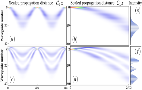
Figure 1: Light intensity propagation in a photonic lattice obtained by integrating Eq. (1). Light is initially launched into a single waveguide labeled as $m=0$ (a), (b) and $m=2$ (c),(d). In (e),(f) we show the output light intensity $I_{m}$$(Z)=|\mathcal{E}_{m}(Z)|^{2}$ at $Z=3\pi/2$ for the simulations presented in (b), (d), respectively. Note, $Z\equiv\mathcal{C}_{1}z$ is the scaled propagation distance. $I_{m}(Z)$ exhibits $m$ nodes as expected from to the probability distribution of the non-classical displaced Fock states Keil et al. (2011). When the ramping potential is activated, $\alpha\neq 0$, we see Bloch-like oscillations Stützer et al. (2017) (left), where the light exhibits revivals every period $Z_{\rm rev}=2\pi k\mathcal{C}_{1}/\alpha$ with $k$ being an integer  Keil et al. (2012). We have set the ratio $\alpha/\mathcal{C}_{1}=1/2$ in (a),(c) and $\alpha/\mathcal{C}_{1}=0$ in (b),(d), which are feasible experimental values that would allow us to implement realistic integrated photonic devices occupying few centimeter-scale footprints, see the text for more details.

Fig. (1) depicts the intensity propagation in a GF lattice of 40 waveguides emulating the unitary evolution of the driven quantum harmonic oscillator. Clearly, we see two scenarios where the light spreads over the entire photonic array (delocalization) Keil et al. (2011) and another in which it strongly localizes as a manifestation of the so called Bloch-like oscillations Stützer et al. (2017). The analytical solution of Eq. (1) can be found in Ref. Keil et al. (2012) in terms of the associated Laguerre polynomials. As a function of the scaled (or normalized) distance $Z\equiv\mathcal{C}_{1}z$, the behavior of $\mathcal{E}_{m}(Z)$ simply depends on the ratio $\alpha/\mathcal{C}_{1}$, and the so-called revival distance $Z_{\rm rev}$ is given as $Z_{\rm rev}=2\pi k\mathcal{C}_{1}/\alpha$. Note that the difference in the case $\alpha>\mathcal{C}_{1}$ as compared to $\alpha<\mathcal{C}_{1}$ is the period of the Bloch-like oscillations, which is short in the former case. Here, to be in accordance with the reported experimental values of $\alpha$ and $\mathcal{C}_{1}$ in previous works, we adopt the latter case. These are simple examples showing the typical dynamics of coherent energy transport in closed systems where strong interference effects dominate. However, when dynamical disorder mechanisms are considered in an open system description, a more involved study of the incoherent energy transport dynamics is necessary, which we aim to cover in the following sections.

II.2 Open dynamics: Markovian master equation

Under the action of Markovian dephasing the density matrix $\hat{\rho}$ of the harmonic oscillator described by the Hamiltonian $\hat{H}=\hbar\omega\hat{n}+\hbar g(\hat{a}+\hat{a}^{\dagger})$ obeys the phenomenological master equation ${d\hat{\rho}}/{dt}=-i[\hat{H},\hat{\rho}]+\gamma\hat{\mathcal{L}}[\hat{n}]\hat{\rho}$. Here the second term on the right hand side is the standard Lindblad superoperator given by $\hat{\mathcal{L}}[\hat{x}]\hat{\rho}\equiv\hat{x}\hat{\rho}\hat{x}^{\dagger}-\frac{1}{2}(\hat{x}^{\dagger}\hat{x}\hat{\rho}+\hat{\rho}\hat{x}^{\dagger}\hat{x})$ with $\gamma$ being the constant dephasing rate. This master equation can be derived using standard techniques of open quantum systems, where the usual Born and Markov approximations are used Breuer and Petruccione (2002).

In general, pure dephasing processes are energy preserving Carmichael (1999), as a result, the interaction between the system and its environment commutes with the unperturbed Hamiltonian of the system, $\omega\hat{n}$ in the present case. To obtain the master equation we compute the matrix elements $\langle n|\hat{H}\hat{\rho}|m\rangle=\omega n\rho_{nm}+\sum_{r}gV_{nr}\rho_{rm}$, with $V_{rm}\equiv\langle r|\left(\hat{a}+\hat{a}^{\dagger}\right)|m\rangle=(\sqrt{m}\delta_{rm-1}+\sqrt{m+1}\delta_{rm+1})$, a similar expression is obtained for $\langle n|\hat{\rho}\hat{H}|m\rangle$. The matrix elements for the dephasing term are

$$\gamma\langle n|\hat{\mathcal{L}}[\hat{n}]\hat{\rho}|m\rangle=\sqrt{\gamma}n\sqrt{\gamma}m\rho_{nm}-\rho_{nm}(\gamma n^{2}+\gamma m^{2})/2.$$ (2)

Therefore, we obtain

$$i \frac{d}{dt}\rho_{nm}=\big{[}(\omega n-\omega m)-\frac{i}{2}(\gamma n^{2}+\gamma m^{2})\big{]}\rho_{nm}$$ (3)

$$+i\sqrt{\gamma}n\sqrt{\gamma}m\rho_{nm}-{\sum}_{r}gV_{rm}\rho_{nr}+{\sum}_{r}gV_{nr}\rho_{rm}.$$

Defining the variables $\omega_{n}\equiv n\omega$, $\gamma_{n}\equiv\gamma n^{2}$ and $v_{ij}\equiv gV_{ij}$, we can rewrite Eq. (3) as

$$i\frac{d}{dt}\rho_{nm} =\Big{[}\big{(}\omega_{n}-\omega_{m}\big{)}-\frac{i}{2}\big{(}\gamma_{n}+\gamma_{m}\big{)}\Big{]}\rho_{nm}+i\sqrt{\gamma_{n}\gamma_{m}}\rho_{nm}$$ (4)

$$\qquad-{\sum}_{r}v_{rm}\rho_{nr}+{\sum}_{r}v_{nr}\rho_{rm},$$

which is the same master equation that a single particle, or excitation, follows during its time evolution in a quantum network affected by non-dissipative noise, as we show in the following section (see also Eq. (1) of Ref. Perez-Leija et al. (2018)). Since Eq. (4) describes a pure-dephasing process only the off-diagonal matrix elements of $\hat{\rho}$ are affected by the constant dephasing rate $\gamma$. Notice that the form of $\gamma_{n}\equiv\gamma n^{2}$ implies that Fock states with high $n$ are more severely affected by dephasing.

III Single-particle dynamics in a network affected by Markovian noise

In this section, we show the equivalence between Eq. (3) [or alternatively Eq. (4)] and the master equation governing the evolution (or propagation) of a single particle in a tight-binding quantum network composed of $N$ coupled sites affected by a stochastic non-dissipative noise (pure dephasing). In the following and throughout the whole paper, keep in mind that with the correspondence between the spatial ($z$) and temporal ($t$) variables, the integrated photonic lattices discussed in the previous section would be a particular case of such networks. In order to establish this connection we begin by writing the single-particle tight-binding Hamiltonian

$$\hat{H}_{S}={\sum}_{n=1}^{N}\omega_{n}(t)|n\rangle\langle n|+{\sum}_{j<n}^{N}\kappa_{jn}(|j\rangle\langle n|+|n\rangle\langle j|),$$ (5)

such that the evolution of the single-particle wavefunction, $\psi_{n}$, at the $n$th site is governed by the stochastic Schrödinger equation

$$\frac{d\psi_{n}}{dt}=-i\omega_{n}(t)\psi_{n}-i{\sum}_{j\neq n}\kappa_{nj}\psi_{j},$$ (6)

where $\kappa_{nj}$ represents, in principle, an arbitrary hopping rate between sites $n$ and $j$. $\omega_{n}(t)=n\big{(}\omega+\phi_{n}(t)\big{)}$ is the frequency at the $n$th site that is affected by the random fluctuations $\phi_{n}(t)$. Note each site exhibits a different natural frequency that changes linearly with $n$, namely $\omega n$. In most of the literature dealing with stochastic quantum networks all sites have the same frequency. However, since our main goal is to establish a connection between the present physical setting and the one describing a driven HO, outlined in Sec. II.2, we chose the frequency of the $n$th site to be proportional to $n$. To introduce pure dephasing we consider $\phi_{n}(t)$ to be a Gaussian stochastic process with a zero mean, $\langle\phi_{n}(t)\rangle=0$, and two-point correlation function given as

$$\qquad\qquad\langle\phi_{n}(t)\phi_{m}(t^{\prime})\rangle=\Gamma\delta_{nm}\delta(t-t^{\prime}),$$ (7)

where $\Gamma$ is the noise strength (dephasing rate) that we have assumed to be the same for all sites. The Kronecker delta $\delta_{nm}$ implies that the noise is uncorrelated between sites $n$ and $m$, the Dirac delta function $\delta(t-t^{\prime})$ describes the Markovian nature (white noise) of the stochastic process, and $\langle...\rangle$ denotes the average over all possible noise realizations. Next, following Ref. de J León-Montiel et al. (2019) we derive the corresponding master equation for the density matrix

$$i \frac{d}{dt}\sigma_{nm}=\big{[}(n\omega-m\omega)-\frac{i}{2}(\Gamma n^{2}+\Gamma m^{2})\big{]}\sigma_{nm}$$ (8)

$$+i\sqrt{\Gamma}n\sqrt{\Gamma}m\delta_{nm}\sigma_{nm}-{\sum}_{j}\kappa_{jm}\sigma_{nj}+{\sum}_{j}\kappa_{nj}\sigma_{jm},\quad$$

where $\sigma_{nm}(t)\equiv\langle\psi_{n}\psi_{m}^{*}\rangle$, see appendix A. Adopting the notation, $\omega_{n}=n\omega$ and $\Gamma_{n}=\Gamma n^{2}$, we obtain

$$i \frac{d}{dt}\sigma_{nm}=\Big{[}\big{(}\omega_{n}-\omega_{m}\big{)}-\frac{i}{2}\big{(}\Gamma_{n}+\Gamma_{m}\big{)}\Big{]}\sigma_{nm}$$ (9)

$$+i\sqrt{\Gamma_{n}\Gamma_{m}}\delta_{nm}\sigma_{nm}-{\sum}_{j}\kappa_{jm}\sigma_{nj}+{\sum}_{j}\kappa_{nj}\sigma_{jm}.$$

Notice that the only difference between Eq. (9) and Eq. (4) is the Kronecker delta $\delta_{nm}$ appearing in the second term on the right-hand-side of Eq. (9). This difference emerges from the fact that we have assumed no correlation between noise affecting different sites, see Eq. (7). However, Eq. (4) and Eq. (9) become identical (no Kronecker delta in Eq. (9)) if we assume $\langle\phi_{n}(t)\phi_{m}(t^{\prime})\rangle=\Gamma\delta(t-t^{\prime})$, i.e., there must be a correlation between stochastic processes at different sites. Such correlation condition, which at first glance seems unlikely to achieve in practice, can easily be emulated using laser written photonic lattices in which temporal correlations are translated into longitudinal spatial correlations. In these photonic devices, ultra-short laser pulses are used to inscribe each waveguide (site) with a customized refractive index (propagation constant or site energy) depending on the writing speed Perez-Leija et al. (2018). The random fluctuations (noise) in the refractive index are implemented by modulating the laser’s writing speed during the manufacturing process with a high degree of control, keeping the coupling coefficients unchanged Caruso et al. (2016). Contrary to uncorrelated noise (7), where independent noise generators in each inscribed waveguide are used Caruso et al. (2016); Perez-Leija et al. (2018), for correlated noise between sites ($\delta_{nm}=1$), a single generator would need to be used during each fabrication step of the waveguide array.

Let us emphasize that in GF lattices, the hopping rates must satisfy, as in the previous case, $\kappa_{nj}=g(\sqrt{j}\delta_{nj-1}+\sqrt{j+1}\delta_{nj+1})$ and the time evolution must be interpreted as spatial propagation. The light intensity represents the probability distribution $P_{n}$ but now this is given by the diagonal matrix elements $\rho_{nn}$ and $\sigma_{nn}$.

In Fig. (2) we compare the dynamics generated by numerically integrating Eq. (9) and Eq. (4). Specifically, we present the corresponding diagonal elements, $\sigma_{nn}$ and $\rho_{nn}$, to illustrate the intensity propagation in a dynamically disorder Glauber-Fock photonic lattice. Both master equations were numerically solved using the technique described in  Navarrete-Benlloch (2015). In Fig. (2) one can see that due to the added noise, near the revival distances $\mathcal{C}_{1}z_{\rm rev}=4\pi k$ light delocalization is more prominent. From the experimental point of view this means that one could build photonic waveguide arrays having just one Bloch-like oscillation ($k=1$) and see the desired dephasing effect. In fact, the ratio $\alpha/\mathcal{C}_{1}=1/2$ used in Figs. (1) and (2) can easily be obtained by choosing the coupling between the zeroth and the first waveguide as $\mathcal{C}_{1}=0.88{\rm cm}^{-1}$ Kondakci et al. (2016); Martin et al. (2011) and $\alpha=0.044{\rm mm}^{-1}$ Stützer et al. (2017). The use of these values implies that we should design approximately $40$ nearest-neighbor coupled waveguides with $z_{\rm rev}=4\pi/\mathcal{C}_{1}=14.28{\rm cm}$, which is a feasible scenario. For instance, in Perez-Leija et al. (2013); Biggerstaff et al. (2016); Keil et al. (2011, 2012); Stützer et al. (2013) waveguides arrays of $10{\rm cm}$ to $15{\rm cm}$ long were built, and in Kondakci et al. (2016); Martin et al. (2011), $101$ identical waveguides were inscribed within one of these types of arrays. In the photonic device, the parameter $\mathcal{C}_{m}=\mathcal{C}_{1}\sqrt{m}$ increases with the waveguide’s label, and by using the above parameters we obtain $\mathcal{C}_{40}\approx 5.5{\rm cm}^{-1}$, which corresponds to the largest coupling coefficient reported experimentally in Dreisow et al. (2009). It is worth pointing out that, given the stochastic nature of the process, a certain number of waveguide samples is needed in order to observe the mean density matrix described in Eq. (9). Previous work by two of us Perez-Leija et al. (2018) has shown that this number is approximately $20$. We would also like to mention that reconfigurable electrical oscillator networks de J. León-Montiel et al. (2015); Quiroz-Juárez et al. (2021) and optical tweezer arrays de J. León-Montiel and Quinto-Su (2017); Sánchez-Sánchez et al. (2019) are other viable experimental platforms in which Eq. (9) and the correlated noise condition between different sites can be realized.

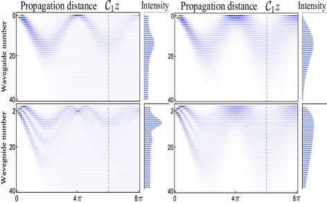
Figure 2: Light propagation in a dynamically disorder Glauber-Fock lattice. On the left we see the diagonal elements $\sigma_{nn}$ obtained by numerical integration of Eq. (9) describing the emerging intensity distribution in the lattice, on the right we depict the matrix elements $\rho_{nn}$ from Eq. (4). For these simulations we used the same parameters and initial conditions as for Figs. (1 $a$,$c$) but now adding white noise with a dephasing rate $\Gamma=0.001$ (left) and $\gamma=0.025$ (right). Due to the noise, light starts to delocalize and the effect is more prominent in the regions where complete Bloch-like oscillations would appear in the absence of noise, see Fig. (1). Vertical dashed line indicates the distance at which the light intensity is calculated.

IV Time-dependent dephasing rate in the master equation

We now turn our attention to generalize the results obtained in the previous section to the case of time-dependent dephasing. This opens up the possibility to introduce memory effects in the dynamics of both models, that is, it enables investigations of non-Markovian effects.

IV.1 Glauber-Fock oscillator

The master equation, in the Lindblad form, for the Hamiltonian $\hat{H}$ under a time-dependent dephasing noise is given as

$$\frac{d\hat{\rho}}{dt}=-i[\hat{H},\hat{\rho}]+\gamma(t)\hat{\mathcal{L}}[\hat{n}]\hat{\rho}.$$ (10)

This equation is an ad hoc generalization of the master equation of a two-level system describing pure-dephasing dynamics in a possibly non-Markovian regime (see Eq. (9) of Ref. Yu and Eberly (2010) and Eq. (17) of Ref. Addis et al. (2014)). In cases where $\gamma(t)$ becomes negative, the quantum dynamical semigroup property of Eq. (10) no longer holds Breuer and Petruccione (2002). Consequently, the divisibility of the quantum map is broken and Eq. (10) can be classified as non-Markovian Addis et al. (2014); Hall et al. (2014). Here, we only consider cases in which $\gamma(t)$ is non-negative. However, it is worth pointing out that Eq. (10) can be used to describe the dynamics of the system under non-Markovian environments provided the dephasing rates exhibit finite environment correlation times  Yu and Eberly (2010); Kumar et al. (2018).
From Eq. (10), and following the same steps as in the previous section, we obtain the master equation

$$i\frac{d}{dt}\rho_{nm}=\Big{[}\big{(}\omega_{n}-\omega_{m}\big{)}-\frac{i}{2}\big{(}\gamma_{n}(t)+\gamma_{m}(t)\big{)}\Big{]}\rho_{nm}$$

$$+i\sqrt{\gamma_{n}(t)\gamma_{m}(t)}\rho_{nm}-{\sum}_{r}\kappa_{rm}\rho_{nr}+{\sum}_{r}\kappa_{nr}\rho_{rm}.\quad$$ (11)

It is interesting to note that the only difference between this expression and Eq. (4) is the time-independent $\gamma_{n}$ which is now replaced by $\gamma_{n}(t)\equiv\gamma(t)n^{2}$. In what follows, we discuss its effect in the transport dynamics of complex quantum networks.

IV.2 Single-particle dynamics in a quantum network

We start by investigating the dynamics of a single particle under the influence of a Gaussian non-Markovian stochastic noise $\Omega_{n}(t)$, with zero mean $\langle\Omega_{n}(t)\rangle=0$ and two-point correlation function

$$2\left\langle\Omega_{n}(t)\Omega_{m}(t^{\prime})\right\rangle={\Gamma\lambda}\delta_{nm}e^{-\lambda|t-t^{\prime}|}.$$ (12)

This is the well known modified Ornstein-Uhlenbeck noise (OUN), where $\Gamma$ is the inverse relaxation time and $\lambda$ is the noise bandwidth which is related to the environmental memory time in the following way $\tau_{c}=\lambda^{-1}$, such that when $\lambda$ is finite the $\tau_{c}$ is also finite giving a non-Markovian character to the dynamics (see Eq. (3) of Yu and Eberly (2010) and Eq. (2.9) of Ref. Kumar et al. (2018) for a detailed discussion on OUN). This process has a well defined Markovian limit which is obtained when $\lim_{\lambda\rightarrow\infty}\langle\Omega_{n}(t)\Omega_{m}(t^{\prime})\rangle=\Gamma\delta_{nm}\delta(t-t^{\prime})$ Yu and Eberly (2010) .
As shown in appendix A, for the present case we obtain the equation

$$\frac{d}{dt}\sigma_{nm}=-i(n\omega-m\omega)\sigma_{nm}-i{\sum}_{j\neq n}\kappa_{nj}\sigma_{jm}$$

$$+i{\sum}_{j\neq m}\kappa_{jm}\sigma_{nj}-in\langle\psi_{n}\psi_{m}^{*}\Omega_{n}(t)\rangle+im\langle\psi_{n}\psi_{m}^{*}\Omega_{m}(t)\rangle,$$

where the matrix elements are given as $\sigma_{nm}=\langle\psi_{n}\psi_{m}^{*}\rangle$.
Although $\Omega_{n}(t)$ represents in general non-Markovian noise it is still a Gaussian process, therefore, we can use the Novikov’s theorem Novikov (1965) to compute the elements

$$\langle\psi_{n}\psi_{m}^{*}\Omega_{n}(t)\rangle\approx-\frac{i}{2}n\sigma_{nm}(t)\Gamma(t)+\frac{i}{2}m\delta_{mn}\sigma_{nm}(t)\Gamma(t),$$ (14)

where $\Gamma(t)\equiv{\Gamma}(1-e^{-\lambda t})/2$, is, basically, the time integral of the two-point correlation function of the environment Yu and Eberly (2010), see appendix B for details. Hence, Eq. (IV.2) becomes

$$i\frac{d}{dt}\sigma_{nm}=\Big{[}\big{(}\omega_{n}-\omega_{m}\big{)}-\frac{i}{2}\big{(}\Gamma_{n}(t)+\Gamma_{m}(t)\big{)}\Big{]}\sigma_{nm}$$

$$+i\sqrt{\Gamma_{n}(t)\Gamma_{m}(t)}\delta_{nm}\sigma_{nm}-{\sum}_{r}\kappa_{rm}\sigma_{nr}+{\sum}_{r}\kappa_{nr}\sigma_{rm},$$

where $\Gamma_{n}(t)\equiv\Gamma(t)n^{2}$. This is the master equation and describes the dynamics of a single particle in a non-Markovian environment and, as expected, it reduces to Eq. (9) when $\Gamma(t)$ is time-independent.

Similarly to the case of Markovian noise, discused in the previous section, the only difference between Eq. (IV.2) and Eq. (IV.1) is the additional Kronecker delta appearing in Eq. (IV.2). That is, when there are noise correlations between different sites then $\rho_{nm}$ and $\sigma_{nm}$ become identical. Even though they exhibit similar evolution, $\rho_{nm}$ and $\sigma_{nm}$ are of a different nature. In other words, $\rho_{nm}$ is the density matrix for a quantum harmonic oscillator inhabiting in an infinite dimensional Hilbert space spanned by an infinite number of Fock states. In contrast, $\sigma_{nm}$ is the density matrix of a single particle, or excitation, evolving in a quantum network made out of finite number of coupled sites, with their corresponding Hilbert space.

Finally, we would like to stress that the derivation of Eqs. (9) and (IV.2) is, in principle, valid for arbitrary time-independent hopping rates $\kappa_{rm}$ and not only for nearest-neighbor interactions. Therefore, these master equations may describe an extensive class of complex networks that do not necessarily have to be photonic.

V Average energy of the system

V.1 Analytical solution for the Markovian case

In this section we discuss some advantages of having a correspondence between the master equations of a driven quantum harmonic oscillator and a single particle propagating in a photonic network. When one is interested in computing the average of certain observables, e.g. the average energy of a particle propagating in a network, solving the HO master equation is much simpler than solving the latter. For example, if we insert the Hamiltonian describing the Glauber-Fock oscillator $\hat{H}_{\texttt{GF}}\equiv\omega\hat{n}+g(\hat{a}+\hat{a}^{\dagger})$ into Eq. (10), we readily obtain the equations of motion for the average of the number and field operators

$$\frac{d\langle\hat{n}\rangle}{dt}=-ig\langle\hat{a}^{\dagger}\rangle+ig\langle\hat{a}\rangle,\,\,\frac{d\langle\hat{a}\rangle}{dt}=\left(-i\omega-\gamma(t)\right)\langle\hat{a}\rangle-ig,$$

where ${d\langle\hat{a}^{\dagger}\rangle}/{dt}={d\langle\hat{a}\rangle^{*}}/{dt}$. In the absence of dephasing, $\gamma(t)=0$, and assuming the initial condition $|\psi(0)\rangle=|m\rangle$, these equations reduce to the well-known solution for the average of the number operator $\langle\hat{n}(t)\rangle=m+({2g}/{\omega})^{2}\sin^{2}(\omega t/2)$. From this expression, one can directly determine the time at which the states return to its initial configuration (revival time) $t_{\mathtt{rev}}=2\pi k/\omega$, with $k$ being an integer. Further, in the limit $\omega\rightarrow 0$, the evolution operator becomes the Glauber displacement displacement operator, $D(\alpha)=\exp(\alpha\hat{a}-\alpha^{*}a^{\dagger})$ with $\alpha=igt$, that transforms a vacuum initial state into a coherent state Keil et al. (2011). Accordingly, in this limit we have $\lim_{\omega\rightarrow 0}\langle\hat{n}(t)\rangle\sim(gt)^{2}$, which corresponds to the average value of a coherent state. For the case of non-dissipative (pure dephasing) Markovian noise the dephasing rate is a non-negative constant $\gamma\neq 0$. Then, the average for the number operator is

$$\langle\hat{n}(t)\rangle = m+\frac{2g^{2}}{(\omega^{2}+\gamma^{2})^{2}}\big{(}f(t)+e^{-\gamma t}g(t)\big{)},$$ (17)

where we have defined the functions $f(t)\equiv\gamma^{2}(\gamma t-1)+\omega^{2}(\gamma t+1)$ and $g(t)\equiv(\gamma^{2}-\omega^{2})\cos(\omega t)-2\gamma\omega\sin(\omega t)$. It is remarkable that the temporal behavior of $\langle\hat{n}(t)\rangle$ in the quantum system gives crucial information about the energy transport across all sites in the photonic structure at fixed propagation distance Román-Ancheyta et al. (2017). This is because $\langle\hat{n}(t)\rangle$ can be rewritten as $\langle\hat{n}(t)\rangle=\sum_{n}P_{n}(t)n$, where $P_{n}(t)=\rho_{nn}(t)$ is the probability distribution that we are associating with the light intensity $I_{n}(z)$ on each waveguide of the photonic lattice. So, in GF lattices, $I_{n}(z)$ is measured first and then the quantitiy $\langle\hat{n}(z)\rangle_{\rm class}\equiv\sum_{m=0}^{N}mI_{m}(z)$ is evaluated. This corresponds to the classical analog of the average photon number in waveguide arrays. Evaluating $\langle\hat{n}(t)\rangle$ at the revival time (revival distance in the GF lattice) yields

$$\langle\hat{n}(t_{\mathtt{rev}})\rangle=m+\frac{2g^{2}}{\omega^{2}}\Big{[}\frac{2\pi k\tilde{\gamma}}{1+\tilde{\gamma}^{2}}+\frac{1-\tilde{\gamma}^{2}}{(1+\tilde{\gamma}^{2})^{2}}\big{(}1-e^{-2\pi k\tilde{\gamma}}\big{)}\Big{]},$$

where $\tilde{\gamma}=\gamma/\omega$ is the scaled dephasing rate and $m$ is the initially excited site. Note $\langle\hat{n}(t_{\mathtt{rev}})\rangle$ attains its maximum value when the decoherence rate is comparable to the energy scale of the system, i.e., when $\tilde{\gamma}\sim 1$ Eq. (V.1) reduces to $\langle\hat{n}(t_{\rm rev})\rangle_{\mathtt{max}}\sim m+2\pi k\left({g}/{\omega}\right)^{2}$. This result indicates that independently of the initial condition (excited site) $|m\rangle$, the delocalization of the initial excitation will increase linearly, as a function of $k$, at each revival time (distance) as shown in Fig. (3).

The Bell-like shape depicted in Fig. (3) is in fact a signature of the so-called environment assisted transport phenomenon, which in the present case is symmetric with respect to the scaled dephasing rate. Note that this result contrasts with the asymmetric behavior typically observed in other coupled-oscillator systems Román-Ancheyta et al. (2017); Maier et al. (2019); de J. León-Montiel and Torres (2013).

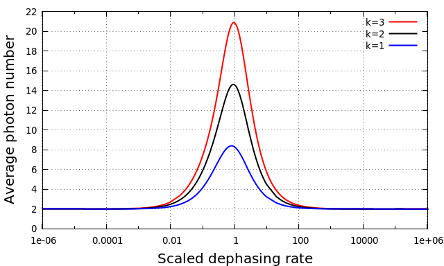
Figure 3: Manifestation of the noise assisted transport phenomenon, captured by the average photon number of Eq. (V.1), as a function of the scaled dephasing rate $\tilde{\gamma}=\gamma/\omega$ at different scaled revivals times counted by $k$, ratio $g/\omega=1$ and initial condition $m=2$.

In general, there are two distinct regimes in systems exhibiting noise-assisted transport. For small dephasing rate, $\tilde{\gamma}\ll 1$, the energy transport is proportional to $\tilde{\gamma}$, such that Eq. (V.1) reduces to $\langle\hat{n}(t_{\rm rev})\rangle\sim m+4\pi k({g}/{\omega})^{2}\tilde{\gamma}$. On the other hand, when the dephasing rate is very high, $\tilde{\gamma}\gg 1$, the energy transport decreases with $1/\tilde{\gamma}$, in fact, it is easy to show that $\langle\hat{n}(t_{\rm rev})\rangle\sim m+4\pi k({g}/{\omega})^{2}{\tilde{\gamma}}^{-1}$. These regimes are shown in Fig. (4), see black solid lines. The fact that the energy transport has a nonmonotonic behavior can be understood, in a quantum scenario, as a consequence of the quantum Zeno effect (QZE)  Fröml et al. (2019). In the QZE a frequent measurement on a quantum system inhibits transitions between quantum states Misra and Sudarshan (1977). In our system the QZE is dominant when the dephasing rate is extremely high, i.e, when the non-disipative noise acts as the measurement process.

In the corresponding optical context of waveguide arrays, the above effects are expected to occur at the revival distance, under the assumptions of couplings coefficients without disorder and no losses in the waveguide array. However, that is not the case in practical implementations. For example, in the presence of static disorder Anderson localization of light will occur for large disorder values as experimentally demonstrated in Martin et al. (2011) for $\alpha=0$, i.e., without Bloch oscillations. When static disorder and Bloch oscillations are both present, Hybrid Bloch-Anderson localization of light emerges with gradual washing out of Bloch oscillations Stützer et al. (2013). Nevertheless, in such case, the first Bloch-like revival (the one we have required to be present in this work) is still visible Stützer et al. (2013). Hence, we deduce that our results are robust against static disorder. On the other hand, a typical experiment of this kind shows low losses. To be more specific, propagation losses are in the range of 0.1$-$0.9${\rm dB~{}cm}^{-1}$ for straight sections of the waveguides and also there is an excellent mode overlap with standard fibers ($0.1\,{\rm dB~{}cm}^{-1}$) Gräfe et al. (2016); Gräfe and Szameit (2020); Perez-Leija et al. (2018). Moreover, losses are approximately independent of the writing speed Szameit and Nolte (2010).

Before concluding this subsection, we would like to point out that while we have assumed zero temperature conditions for the driven quantum harmonic oscillator, there is no restriction for considering temperature effects upon the photonic lattices structures. Most experiments using direct laser-written waveguides are performed at room temperature Szameit and Nolte (2010); Gräfe et al. (2016). Moreover, impressive thermal effects can be admitted on these devices. For instance, in Pertsch et al. (1999), it was experimentally shown that varying a temperature gradient, the Bloch oscillations’ period and amplitude could be controlled. This can be done by heating and cooling the opposite sides of the waveguide array. Specifically, a transverse linear temperature gradient $\Delta T$ leads to a linear variation of the propagation constants, i.e., $\alpha\propto\Delta T$. Such result suggests an attractive alternative to get the desired ramp potential or the random fluctuations without changing the laser’s writing speed.

V.2 Numerical solution for the non-Markovian case

We now look into the numerical solutions of the equations of motion for the average field and number operators under two different types of non-Markovian noise models. We consider Ornstein-Uhlenbeck noise (OUN) and power law noise (PLN), both of which have a well defined Markovian limit. The time-dependent dephasing rates for these cases are given as Kumar et al. (2018); Utagi et al. (2020)

$$\Gamma(t)=\begin{cases}\frac{\Gamma}{2}(1-e^{-\lambda t})&\text{OUN},\\ \frac{\Gamma}{2(\lambda t+1)^{3}}&\text{PLN},\end{cases}$$ (19)

where $\Gamma$ is the inverse relaxation time and $\lambda$ and $1/\lambda$ are the noise bandwidths for OUN and PLN, respectively, which in turn are related to the finite correlation time of the environment. Note these quantities can be considered as the inverse environmental memory time that vanish in the limit of $\lambda\rightarrow\infty$ and $1/\lambda\rightarrow\infty$ for OUN and PLN, respectively, yielding the Markovian limits of these noise models. Naturally, in the Markovian limit, the time-dependent dephasing factors become time-independent. It is important to note that in both cases $\Gamma(t)$ never becomes negative throughout the evolution. Therefore, the dynamics generated are CP-divisible at all times and considered as Markovian Rivas et al. (2014); Breuer et al. (2016). Nevertheless, it is clear that finite environment correlation time results in non-Markovian behavior in the dynamics Yu and Eberly (2010); Kumar et al. (2018), such that any intermediate map taking the system from $t_{1}$ to $t_{2}$, is not independent of the initial time $t_{0}$. It has been shown that it is also possible to quantify these “weaker” forms of non-Markovianity emerging in these models, by adopting different strategies as shown in Utagi et al. (2020).

(a)

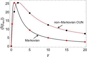
(b)

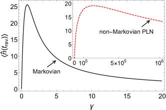
Figure 4: Noise-assisted transport phenomenon in a Glauber-Fock oscillator (lattice) as a function of the dephasing rate, $\gamma$, under (a) Ornstein-Uhlenbeck noise (OUN) and (b) power law noise (PLN). The system was prepared initially in ground state $|0\rangle$, i.e., $m=0$, $g=1$, $\omega=0.5$ and $k=1$. For (a) ((b)) $\lambda\rightarrow\infty$ ($\lambda^{-1}\rightarrow\infty$) black solid line corresponds to the Markovian limit given by Eq. (V.1), and $\lambda^{-1}={\color[rgb]{0,0,0}10}$ ($\lambda={\color[rgb]{0,0,0}10}$) red dashed line shows the behavior in the non-Markovian regime evaluating Eq. (V.1) at $t_{\rm rev}$. We obtain the red (black) circular (square) dots by integrating the master equation (IV.1).

In Utagi et al. (2020), the authors provide a geometric measure of non-Markovianity that is capable of capturing the amount of non-Markovianity for the CP-divisible models considered above and provide a comparative analysis. Fixing $x=\lambda^{-1}$ for OUN and $x=\lambda$ for PLN, it has been shown that the non-Markovianity of PLN is always higher than that of OUN for any finite $x$ (cf. Fig. 1-(a) of  Utagi et al. (2020)). Note that $x=0$ corresponds to the case $\lambda\rightarrow\infty$ for OUN and $1/\lambda\rightarrow\infty$ for PLN, which are the Markovian limits of these models. We set $x={\color[rgb]{0,0,0}10}$ and look at the noise-assisted transport phenomenon in a Glauber-Fock oscillator (lattice) under OUN and PLN noise, together with their corresponding Markovian limit. Fig. (4) shows that for this value, $x={\color[rgb]{0,0,0}10}$, which corresponds to $\lambda={\color[rgb]{0,0,0}0.1}$ for OUN and $\lambda={\color[rgb]{0,0,0}10}$ for PLN, the noise-assisted transport phenomenon shows a higher enhancement over a broader range of dephasing in the case of PLN as compared to OUN, which also presents a higher non-Markovianity.

In Fig. 4$(a)$, we show that the pure numerical calculation of the master equation (IV.1) coincides (as expected) with the solution of Eq. (V.1), but the latter is significantly more straightforward to solve than the former. Interestingly, even when we do not consider correlations between sites, one can still observe the enhancement in noise-assisted transport in the non-Markovian case described by the master equation (IV.2). This suggests that for the specific model of GF oscillator (lattice) considered in this work, non-Markovianity seems quite advantageous in the noise-assisted transport phenomenon. Increased non-Markovianity in the open system dynamics, allows us to achieve finite $\langle\hat{n}(t)\rangle$, or equivalently $\langle\hat{n}(z)\rangle_{\rm class}$, for larger values of the dephasing rate. Although our findings are limited to the models considered in this work, they are in accordance with recent results in the literature that show positive correlation between non-Markovianity and noise-assisted transport efficiencies Trautmann and Hauke (2018); Maier et al. (2019); Moreira et al. (2020).

VI Conclusions

We have explored the conditions under which the master equation describing a driven quantum harmonic oscillator, interacting with an environment in a non-dissipative way, is equivalent to the master equation describing light propagation in a dynamically disordered photonic lattice – the Glauber-Fock photonic lattice. One of these conditions is that the noise between different sites (waveguides) must be correlated. The second condition is to choose a number of waveguides such that the light do not reach the boundary where the sites corresponding to high number states lie. Further, we have shown that the noise-assisted energy transport phenomenon can be observed in this type of systems and that it is possible to obtain analytical solutions for certain observables quantities, e.g. the average photon number. Using these solutions we can readily predict the maximum amount of energy transferred between all the sites. This, in the Markovian scenario, occurs for decoherence rates comparable to the energy scale of the system. For the non-Markovian case, we found that the range of the dephasing rate, in which the noise-assisted transport occurs, is substantially larger. Our results are in good agreement with recent theoretical Moreira et al. (2020); Trautmann and Hauke (2018) and experimental Maier et al. (2019) works showing that non-Markovian environments have a strong influence on the energy transport. Looking forward, and following the ideas of Refs. Perez-Leija et al. (2017); de J León-Montiel et al. (2019), it would be interesting to go beyond the single excitation regime and derive the corresponding master equation of, for example, two correlated particles propagating over these stochastic networks affected by non-Markovian noise.

Appendix A

The time derivative of the density matrix $\sigma_{nm}(t)\equiv\langle\psi_{n}\psi_{m}^{*}\rangle$ is given as

$$\frac{d}{dt}\sigma_{nm}=\Big{\langle}\psi_{m}^{*}\frac{d\psi_{n}}{dt}+\psi_{n}\frac{d\psi_{m}^{*}}{dt}\Big{\rangle},$$ (20)

where each term can be calculated using the stochastic Schrödinger equation:

$$\psi_{m}^{*}\frac{d\psi_{n}}{dt}=-in\omega\psi_{n}\psi_{m}^{*}- in\phi_{n}(t)\psi_{n}\psi_{m}^{*}$$ (21a)

$$-i\sum_{j\neq n}\kappa_{nj}\psi_{j}\psi_{m}^{*},$$

$$\psi_{n}\frac{d\psi_{m}^{*}}{dt}=+im\omega\psi_{n}\psi_{m}^{*}+ im\phi_{m}(t)\psi_{n}\psi_{m}^{*}$$ (21b)

$$+i\sum_{j\neq m}\kappa_{jm}\psi_{n}\psi_{j}^{*}.$$

Performing the stochastic averaging procedure these terms yield

$$\frac{d}{dt}\sigma_{nm}=-i(n\omega-m\omega)\sigma_{nm}-i\sum_{j\neq n}\kappa_{nj}\sigma_{jm}$$

$$+i{\sum}_{j\neq m}\kappa_{jm}\sigma_{nj}-in\langle\psi_{n}\psi_{m}^{*}\phi_{n}(t)\rangle+im\langle\psi_{n}\psi_{m}^{*}\phi_{m}(t)\rangle.$$

In particular, the stochastic averages in the last two terms of the above equation, one needs to resort to the Novikov’s theorem Novikov (1965):

$$\langle\psi_{n}\psi_{m}^{*}\phi_{n}(t)\rangle =\sum_{p}\int dt^{\prime}\langle\phi_{n}(t)\phi_{p}(t^{\prime})\rangle\left\langle\frac{\delta[\psi_{n}(t)\psi_{m}^{*}(t)]}{\delta\phi_{p}(t^{\prime})}\right\rangle,$$ (23d)

$$=\sum_{p}\int dt^{\prime}\Gamma\delta_{np}\delta(t-t^{\prime})\left\langle\frac{\delta[\psi_{n}(t)\psi_{m}^{*}(t)]}{\delta\phi_{p}(t^{\prime})}\right\rangle,$$

$$=\frac{1}{2}\sum_{p}\Gamma\delta_{np}\left\langle\frac{\delta[\psi_{n}(t)\psi_{m}^{*}(t)]}{\delta\phi_{p}(t)}\right\rangle,$$

$$=\frac{\Gamma}{2}\left\langle\frac{\delta[\psi_{n}(t)\psi_{m}^{*}(t)]}{\delta\phi_{n}(t)}\right\rangle,$$

where the operator $\delta/\delta\phi_{p}(t)$ stands for the functional derivative with respect to the stochastic process. Similarly, the second term can be found as

$$\langle\psi_{n}\psi_{m}^{*}\phi_{m}(t)\rangle=\frac{\Gamma}{2}\left\langle\frac{\delta[\psi_{n}(t)\psi_{m}^{*}(t)]}{\delta\phi_{m}(t)}\right\rangle.$$ (24)

To obtain Eq. (23d) and Eq. (24) we have used the fact that, in the Stratonovich interpretation, $\int\delta(t)=1/2$ van Kampen (1981). It is important to mention that the Novikov’s theorem is only valid for stochastic Gaussian processes, that can be both Markovian or non-Markovian as well Strunz and Yu (2004). To compute the corresponding functional derivatives we need the formal integration of Eq. (A) which, before the stochastic average, is

$$\psi_{n}(t)\psi_{m}^{*}(t)=\int_{0}^{t}dt^{\prime}\Big{[}f (\psi_{n}\psi_{m}^{*},..)-in\psi_{n}\psi_{m}^{*}\phi_{n}(t^{\prime})$$ (25)

$$+im\psi_{n}\psi_{m}^{*}\phi_{m}(t^{\prime})\Big{]},$$

where $f(\psi_{n}\psi_{m}^{*},..)$ represents all the terms that do not contain stochastic variable, $\phi_{n}(t)$. Thus, the functional derivatives are

$$\frac{\delta[\psi_{n}(t)\psi_{m}^{*}(t)]}{\delta\phi_{n}(t)}=-in\psi_{n}\psi_{m}^{*}+im\psi_{n}\psi_{m}^{*}\delta_{nm},\quad$$ (26a)

$$\frac{\delta[\psi_{n}(t)\psi_{m}^{*}(t)]}{\delta\phi_{m}(t)}=-in\psi_{n}\psi_{m}^{*}\delta_{nm}+im\psi_{n}\psi_{m}^{*},\quad$$ (26b)

in which we have use the identity $\delta\phi_{p}(t^{\prime})/\delta\phi_{q}(t)=\delta_{pq}\delta(t^{\prime}-t)$  Novikov (1965). Using these results we can compute the stochastic average for the last two terms in Eq. (A) as

$$-in\langle\psi_{n}\psi_{m}^{*}\phi_{n}(t)\rangle =-\frac{1}{2}\Gamma n^{2}\rho_{nm}+\frac{1}{2}\Gamma nm\rho_{nm}\delta_{nm},\qquad$$ (27a)

$$im\langle\psi_{n}\psi_{m}^{*}\phi_{m}(t)\rangle =\frac{1}{2}\Gamma nm\rho_{nm}\delta_{nm}-\frac{1}{2}\Gamma m^{2}\rho_{nm},\qquad$$ (27b)

and as a result we obtain Eq. (8) of the main text.

Appendix B

Applying the Novikov’s theorem Novikov (1965) in $\langle\psi_{n}\psi_{m}^{*}\Omega_{n}(t)\rangle$ we get:

$$\langle\psi_{n}\psi_{m}^{*}\Omega_{n}(t)\rangle =\sum_{p}\int dt^{\prime}\langle\Omega_{n}(t)\Omega_{p}(t^{\prime})\rangle\left\langle\frac{\delta[\psi_{n}(t)\psi_{m}^{*}(t)]}{\delta\Omega_{p}(t^{\prime})}\right\rangle,$$

$$=\sum_{p}\int dt^{\prime}\frac{\Gamma\lambda}{2}\delta_{np}e^{-\lambda|t-t^{\prime}|}\left\langle\frac{\delta[\psi_{n}(t)\psi_{m}^{*}(t)]}{\delta\Omega_{p}(t^{\prime})}\right\rangle.$$

The final aim of this appendix is to know if the master equation of Eq. (IV.2) of the main text, after applying Novikov’s theorem in Eq. (LABEL:noviko_non_markovian), will be similar to the master equation of Eq. (IV.1). Using the formal integration of Eq. (IV.2), before doing the stochastic average, we can compute the functional derivative of Eq. (LABEL:noviko_non_markovian) as follows

$$\frac{\delta[\psi_{n}(t)\psi_{m}^{*}(t)]}{\delta\Omega_{p}(t^{\prime})} =\frac{\delta}{\delta\Omega_{p}(t^{\prime})}\int_{0}^{t}dt^{\prime\prime}\Big{[}f(\psi_{n}\psi_{m}^{*},..)-in\psi_{n}\psi_{m}^{*}\Omega_{n}(t^{\prime\prime})+im\psi_{n}\psi_{m}^{*}\Omega_{m}(t^{\prime\prime})\Big{]},$$

$$=\int_{0}^{t}dt^{\prime\prime}\Big{[}-in\psi_{n}\psi_{m}^{*}\frac{\delta\Omega_{n}(t^{\prime\prime})}{\delta\Omega_{p}(t^{\prime})}+im\psi_{n}\psi_{m}^{*}\frac{\delta\Omega_{m}(t^{\prime\prime})}{\delta\Omega_{p}(t^{\prime})}\Big{]},$$

$$=\int_{0}^{t}dt^{\prime\prime}\big{[}-in\psi_{n}\psi_{m}^{*}\delta_{np}\delta(t^{\prime\prime}-t^{\prime})+im\psi_{n}\psi_{m}^{*}\delta_{mp}\delta(t^{\prime\prime}-t^{\prime})\big{]},$$

$$=-\frac{i}{2}n\psi_{n}(t^{\prime})\psi_{m}^{*}(t^{\prime})\delta_{np}+\frac{i}{2}m\psi_{n}(t^{\prime})\psi_{m}^{*}(t^{\prime})\delta_{mp}.$$ (29)

Performing the stochastic average in Eq. (29) we obtain

$$\left\langle\frac{\delta[\psi_{n}(t)\psi_{m}^{*}(t^{\prime})]}{\delta\Omega_{p}(t^{\prime})}\right\rangle=-\frac{i}{2}n\delta_{np}\sigma_{nm}(t^{\prime})+\frac{i}{2}m\delta_{mp}\sigma_{nm}(t^{\prime}).$$ (30)

Now we substitute Eq. (30) in Eq. (LABEL:noviko_non_markovian):

$$\langle\psi_{n}\psi_{m}^{*}\Omega_{n}(t)\rangle =\sum_{p}\int dt^{\prime}\frac{\Gamma\lambda}{2}\delta_{np}e^{-\lambda|t-t^{\prime}|}\big{\{}-\frac{i}{2}n\delta_{np}\sigma_{nm}(t^{\prime})+\frac{i}{2}m\delta_{mp}\sigma_{nm}(t^{\prime})\big{\}},$$ (31a)

$$=-\frac{i}{2}n\int dt^{\prime}\frac{\Gamma\lambda}{2}e^{-\lambda|t-t^{\prime}|}\sigma_{nm}(t^{\prime})+\frac{i}{2}m\delta_{mn}\int dt^{\prime}\frac{\Gamma\lambda}{2}e^{-\lambda|t-t^{\prime}|}\sigma_{nm}(t^{\prime}),$$ (31b)

$$\approx-\frac{i}{2}n\sigma_{nm}(t)\int dt^{\prime}\frac{\Gamma\lambda}{2}e^{-\lambda|t-t^{\prime}|}+\frac{i}{2}m\delta_{mn}\sigma_{nm}(t)\int dt^{\prime}\frac{\Gamma\lambda}{2}e^{-\lambda|t-t^{\prime}|},$$ (31c)

where we have made an approximation $\sigma_{nm}(t^{\prime})\approx\sigma_{nm}(t)$, i.e., we assume that the dynamics of the density matrix is slower compared with the dynamics of the stochastic processes. Under this approximation we can perform the integral of the above equation,

$$\int_{0}^{t}dt^{\prime}\frac{\Gamma\lambda}{2}e^{-\lambda|t-t^{\prime}|}=\frac{\Gamma}{2}(1-e^{-\lambda t})\equiv\Gamma(t).$$ (32)

With this result, Eq. (31c) reduces to Eq. (14) of the main text.

References

- Bose (2003) Sougato Bose, “Quantum communication through an unmodulated spin chain,” Phys. Rev. Lett. 91, 207901 (2003).
- Plenio and Huelga (2008) M. Plenio and S. Huelga, “Dephasing-assisted transport: quantum networks and biomolecules,” New J. Phys. 10, 113019 (2008).
- Rebentrost et al. (2009) Patrick Rebentrost, Masoud Mohseni, Ivan Kassal, Seth Lloyd, and Alán Aspuru-Guzik, “Environment-assisted quantum transport,” New Journal of Physics 11, 033003 (2009).
- Kurizki et al. (2015) Gershon Kurizki, Patrice Bertet, Yuimaru Kubo, Klaus Mølmer, David Petrosyan, Peter Rabl, and Jörg Schmiedmayer, “Quantum technologies with hybrid systems,” Proceedings of the National Academy of Sciences 112, 3866–3873 (2015).
- Scully et al. (2011) Marlan O. Scully, Kimberly R. Chapin, Konstantin E. Dorfman, Moochan Barnabas Kim, and Anatoly Svidzinsky, “Quantum heat engine power can be increased by noise-induced coherence,” Proceedings of the National Academy of Sciences 108, 15097–15100 (2011).
- Pezzutto et al. (2019) Marco Pezzutto, Mauro Paternostro, and Yasser Omar, “An out-of-equilibrium non-Markovian quantum heat engine,” Quantum Science and Technology 4, 025002 (2019).
- Román-Ancheyta et al. (2020) Ricardo Román-Ancheyta, Barış Çakmak, and Özgür E. Müstecaplıoğlu, “Spectral signatures of non-thermal baths in quantum thermalization,” Quantum Science and Technology 5, 015003 (2020).
- Salado-Mejía et al. (2021) Mariana Salado-Mejía, Ricardo Román-Ancheyta, Francisco Soto-Eguibar, and Héctor Moya-Cessa, “Spectroscopy and critical quantum thermometry in the ultrastrong coupling regime,” Quantum Science and Technology (2021).
- Szameit and Nolte (2010) Alexander Szameit and Stefan Nolte, “Discrete optics in femtosecond-laser-written photonic structures,” Journal of Physics B: Atomic, Molecular and Optical Physics 43, 163001 (2010).
- Gräfe et al. (2016) Markus Gräfe, René Heilmann, Maxime Lebugle, Diego Guzman-Silva, Armando Perez-Leija, and Alexander Szameit, “Integrated photonic quantum walks,” Journal of Optics 18, 103002 (2016).
- Perez-Leija et al. (2013) Armando Perez-Leija, Robert Keil, Alastair Kay, Hector Moya-Cessa, Stefan Nolte, Leong-Chuan Kwek, Blas M. Rodríguez-Lara, Alexander Szameit, and Demetrios N. Christodoulides, “Coherent quantum transport in photonic lattices,” Phys. Rev. A 87, 012309 (2013).
- Biggerstaff et al. (2016) D. N. Biggerstaff, R. Heilmann, A. A. Zecevik, M. Gräfe, M. A. Broome, A. Fedrizzi, S. Nolte, A. Szameit, A. G. White, and I. Kassal, “Enhancing coherent transport in a photonic network using controllable decoherence,” Nat. Commun. 7, 11282 (2016).
- Bossé and Vinet (2017) Éric-Olivier Bossé and Luc Vinet, “Coherent transport in photonic lattices: a survey of recent analytic results,” SIGMA. Symmetry, Integrability and Geometry: Methods and Applications 13, 074 (2017).
- O’Brien et al. (2009) Jeremy L. O’Brien, Akira Furusawa, and Jelena Vučković, “Photonic quantum technologies,” Nature Photonics 3, 687–695 (2009).
- Wang et al. (2020) Jianwei Wang, Fabio Sciarrino, Anthony Laing, and Mark G. Thompson, “Integrated photonic quantum technologies,” Nature Photonics 14, 273–284 (2020).
- Gräfe and Szameit (2020) Markus Gräfe and Alexander Szameit, “Integrated photonic quantum walks,” Journal of Physics B: Atomic, Molecular and Optical Physics 53, 073001 (2020).
- Breuer and Petruccione (2002) Heinz-Peter Breuer and Francesco Petruccione, The theory of open quantum systems (Oxford University Press on Demand, 2002).
- Perez-Leija et al. (2010) Armando Perez-Leija, Hector Moya-Cessa, Alexander Szameit, and Demetrios N. Christodoulides, “Glauber–Fock photonic lattices,” Opt. Lett. 35, 2409–2411 (2010).
- Rai and Angelakis (2019) Amit Rai and Dimitris G Angelakis, “Quantum light in Glauber-Fock photonic lattices,” Journal of Optics 21, 065201 (2019).
- Keil et al. (2011) Robert Keil, Armando Perez-Leija, Felix Dreisow, Matthias Heinrich, Hector Moya-Cessa, Stefan Nolte, Demetrios N. Christodoulides, and Alexander Szameit, “Classical analogue of displaced Fock states and quantum correlations in Glauber-Fock photonic lattices,” Phys. Rev. Lett. 107, 103601 (2011).
- Keil et al. (2012) Robert Keil, Armando Perez-Leija, Parinaz Aleahmad, Hector Moya-Cessa, Stefan Nolte, Demetrios N. Christodoulides, and Alexander Szameit, “Observation of Bloch-like revivals in semi-infinite Glauber–Fock photonic lattices,” Opt. Lett. 37, 3801–3803 (2012).
- Martínez et al. (2012) A. J. Martínez, U. Naether, A. Szameit, and R. A. Vicencio, “Nonlinear localized modes in Glauber-Fock photonic lattices,” Opt. Lett. 37, 1865–1867 (2012).
- Yuce and Ramezani (2020) Cem Yuce and Hamidreza Ramezani, “Diffraction-free beam propagation at the exceptional point of non-Hermitian Glauber Fock lattices,” (2020), arXiv:2009.12880 [physics.optics] .
- Oztas (2018) Z. Oztas, “Nondiffracting wave beams in non-Hermitian Glauber–Fock lattice,” Physics Letters A 382, 1190 – 1193 (2018).
- Caruso et al. (2016) F. Caruso, A. Crespi, A. G. Ciriolo, F. Sciarrino, and R. Osellame, “Fast escape of a quantum walker from an integrated photonic maze,” Nat. Commun. 7, 11682 (2016).
- Maier et al. (2019) Christine Maier, Tiff Brydges, Petar Jurcevic, Nils Trautmann, Cornelius Hempel, Ben P. Lanyon, Philipp Hauke, Rainer Blatt, and Christian F. Roos, “Environment-assisted quantum transport in a 10-qubit network,” Phys. Rev. Lett. 122, 050501 (2019).
- de J. León-Montiel et al. (2015) R. de J. León-Montiel, M. A. Quiroz-Juárez, R. Quintero-Torres, J. L. Domínguez-Juárez, H. M. Moya-Cessa, J. P. Torres, and J. L. Aragón, “Noise-assisted energy transport in electrical oscillator networks with off-diagonal dynamical disorder,” Sci. Rep. 5, 17339 (2015).
- Viciani et al. (2015) Silvia Viciani, Manuela Lima, Marco Bellini, and Filippo Caruso, “Observation of noise-assisted transport in an all-optical cavity-based network,” Phys. Rev. Lett. 115, 083601 (2015).
- Kassal et al. (2013) Ivan Kassal, Joel Yuen-Zhou, and Saleh Rahimi-Keshari, “Does coherence enhance transport in photosynthesis?” The Journal of Physical Chemistry Letters 4, 362–367 (2013).
- Castaños and Zuñiga-Segundo (2019) L. O. Castaños and A. Zuñiga-Segundo, “The forced harmonic oscillator: Coherent states and the RWA,” American Journal of Physics 87, 815–823 (2019).
- Román-Ancheyta et al. (2017) Ricardo Román-Ancheyta, Irán Ramos-Prieto, Armando Perez-Leija, Kurt Busch, and Roberto de J. León-Montiel, “Dynamical casimir effect in stochastic systems: Photon harvesting through noise,” Phys. Rev. A 96, 032501 (2017).
- Stützer et al. (2017) Simon Stützer, Alexander S. Solntsev, Stefan Nolte, Andrey A. Sukhorukov, and Alexander Szameit, “Observation of Bloch oscillations with a threshold,” APL Photonics 2, 051302 (2017).
- Carmichael (1999) Howard J. Carmichael, “Two-Level Atoms and Spontaneous Emission,” in Statistical Methods in Quantum Optics 1: Master Equations and Fokker-Planck Equations, Texts and Monographs in Physics, edited by Howard J. Carmichael (Springer, Berlin, Heidelberg, 1999) pp. 29–74.
- Perez-Leija et al. (2018) Armando Perez-Leija, Diego Guzmán-Silva, Roberto de J León-Montiel, Markus Gräfe, Matthias Heinrich, Hector Moya-Cessa, Kurt Busch, and Alexander Szameit, “Endurance of quantum coherence due to particle indistinguishability in noisy quantum networks,” npj Quantum Information 4, 45 (2018).
- de J León-Montiel et al. (2019) Roberto de J León-Montiel, Vicenç Méndez, Mario A Quiroz-Juárez, Adrian Ortega, Luis Benet, Armando Perez-Leija, and Kurt Busch, “Two-particle quantum correlations in stochastically-coupled networks,” New Journal of Physics 21, 053041 (2019).
- Navarrete-Benlloch (2015) Carlos Navarrete-Benlloch, “Open systems dynamics: Simulating master equations in the computer,” arXiv preprint arXiv:1504.05266 (2015).
- Kondakci et al. (2016) H. Esat Kondakci, Lane Martin, Robert Keil, Armando Perez-Leija, Alexander Szameit, Ayman F. Abouraddy, Demetrios N. Christodoulides, and Bahaa E. A. Saleh, “Hanbury Brown and twiss anticorrelation in disordered photonic lattices,” Phys. Rev. A 94, 021804 (2016).
- Martin et al. (2011) Lane Martin, Giovanni Di Giuseppe, Armando Perez-Leija, Robert Keil, Felix Dreisow, Matthias Heinrich, Stefan Nolte, Alexander Szameit, Ayman F. Abouraddy, Demetrios N. Christodoulides, and Bahaa E. A. Saleh, “Anderson localization in optical waveguide arrays with off-diagonal coupling disorder,” Opt. Express 19, 13636–13646 (2011).
- Stützer et al. (2013) Simon Stützer, Yaroslav V. Kartashov, Victor A. Vysloukh, Vladimir V. Konotop, Stefan Nolte, Lluis Torner, and Alexander Szameit, “Hybrid Bloch-Anderson localization of light,” Opt. Lett. 38, 1488–1490 (2013).
- Dreisow et al. (2009) F. Dreisow, A. Szameit, M. Heinrich, T. Pertsch, S. Nolte, A. Tünnermann, and S. Longhi, “Bloch-Zener oscillations in binary superlattices,” Phys. Rev. Lett. 102, 076802 (2009).
- Quiroz-Juárez et al. (2021) Mario A. Quiroz-Juárez, Chenglong You, Javier Carrillo-Martínez, Diego Montiel-Álvarez, José L. Aragón, Omar S. Magaña Loaiza, and Roberto de J. León-Montiel, “Reconfigurable network for quantum transport simulations,” Phys. Rev. Research 3, 013010 (2021).
- de J. León-Montiel and Quinto-Su (2017) R. de J. León-Montiel and P. A. Quinto-Su, “Noise-enabled optical ratchets,” Sci. Rep. 7, 44287 (2017).
- Sánchez-Sánchez et al. (2019) M. G. Sánchez-Sánchez, R. de J. León-Montiel, and P. A. Quinto-Su, “Phase dependent vectorial current control in symmetric noisy optical ratchets,” Phys. Rev. Lett. 123, 170601 (2019).
- Yu and Eberly (2010) Ting Yu and J.H. Eberly, “Entanglement evolution in a non-markovian environment,” Optics Communications 283, 676 – 680 (2010).
- Addis et al. (2014) Carole Addis, Bogna Bylicka, Dariusz Chruściński, and Sabrina Maniscalco, “Comparative study of non-markovianity measures in exactly solvable one- and two-qubit models,” Phys. Rev. A 90, 052103 (2014).
- Hall et al. (2014) Michael J. W. Hall, James D. Cresser, Li Li, and Erika Andersson, “Canonical form of master equations and characterization of non-markovianity,” Phys. Rev. A 89, 042120 (2014).
- Kumar et al. (2018) N Pradeep Kumar, Subhashish Banerjee, R Srikanth, Vinayak Jagadish, and Francesco Petruccione, “Non-markovian evolution: a quantum walk perspective,” Open Systems & Information Dynamics 25, 1850014 (2018).
- Novikov (1965) Evgenii A Novikov, “Functionals and the random-force method in turbulence theory,” Sov. Phys. JETP 20, 1290–1294 (1965).
- de J. León-Montiel and Torres (2013) R. de J. León-Montiel and J. P. Torres, “Highly efficient noise-assisted energy transport in classical oscillator systems,” Phys. Rev. Lett. 110, 218101 (2013).
- Fröml et al. (2019) Heinrich Fröml, Alessio Chiocchetta, Corinna Kollath, and Sebastian Diehl, “Fluctuation-induced quantum Zeno effect,” Phys. Rev. Lett. 122, 040402 (2019).
- Misra and Sudarshan (1977) B. Misra and E. C. G. Sudarshan, “The Zeno’s paradox in quantum theory,” Journal of Mathematical Physics 18, 756–763 (1977).
- Pertsch et al. (1999) T. Pertsch, P. Dannberg, W. Elflein, A. Bräuer, and F. Lederer, “Optical Bloch oscillations in temperature tuned waveguide arrays,” Phys. Rev. Lett. 83, 4752–4755 (1999).
- Utagi et al. (2020) Shrikant Utagi, R. Srikanth, and Subhashish Banerjee, “Temporal self-similarity of quantum dynamical maps as a concept of memorylessness,” Scientific Reports 10, 15049 (2020).
- Rivas et al. (2014) Ángel Rivas, Susana F Huelga, and Martin B Plenio, “Quantum non-markovianity: characterization, quantification and detection,” Reports on Progress in Physics 77, 094001 (2014).
- Breuer et al. (2016) Heinz-Peter Breuer, Elsi-Mari Laine, Jyrki Piilo, and Bassano Vacchini, “Colloquium: Non-markovian dynamics in open quantum systems,” Rev. Mod. Phys. 88, 021002 (2016).
- Trautmann and Hauke (2018) N. Trautmann and P. Hauke, “Trapped-ion quantum simulation of excitation transport: Disordered, noisy, and long-range connected quantum networks,” Phys. Rev. A 97, 023606 (2018).
- Moreira et al. (2020) S. V. Moreira, B. Marques, R. R. Paiva, L. S. Cruz, D. O. Soares-Pinto, and F. L. Semião, “Enhancing quantum transport efficiency by tuning non-markovian dephasing,” Phys. Rev. A 101, 012123 (2020).
- Perez-Leija et al. (2017) Armando Perez-Leija, Roberto de J Leon-Montiel, Jan Sperling, Hector Moya-Cessa, Alexander Szameit, and Kurt Busch, “Two-particle four-point correlations in dynamically disordered tight-binding networks,” Journal of Physics B: Atomic, Molecular and Optical Physics 51, 024002 (2017).
- van Kampen (1981) N. G. van Kampen, “Itô versus Stratonovich,” Journal of Statistical Physics 24, 175–187 (1981).
- Strunz and Yu (2004) Walter T. Strunz and Ting Yu, “Convolutionless non-markovian master equations and quantum trajectories: Brownian motion,” Phys. Rev. A 69, 052115 (2004).