Re-estimating the Spin Parameter of the Black Hole in Cygnus X-1

Abstract

Cygnus X-1 is a well-studied persistent black hole X-ray binary. Recently, the three parameters needed to estimate the black hole spin of this system, namely the black hole mass $M$, the orbital inclination $i$ and the source distance $D$, have been updated. In this work we redetermine the spin parameter using the continuum-fitting technique for those updated parameter values. Based on the assumption that the spin axis of the black hole is aligned with the orbital plane, we fit the thermal disk component to a fully relativistic thin accretion disk model. The error in the spin estimate arising from the combined observational uncertainties is obtained via Monte Carlo (MC) simulations. We demonstrate that, without considering the counteracting torque effect, the new spin parameter is constrained to be a${}_{*}>0.9985$ (3$\sigma$), which confirms that the spin of the black hole in Cygnus X-1 is extreme.

1 introduction

The spin parameter is a fundamental physical property of a black hole, which can be estimated observationally using one of two widely-used methods; the iron-line fitting method (Fabian et al. 1989, Reynolds & Nowak 2003) and the continuum-fitting method (Zhang et al. 1997). In this work we use the continuum-fitting method to estimate the dimensionless spin parameter $a_{*}$ ($a_{*}\equiv a/M\equiv cJ/GM^{2}$, where $M$ and $J$ indicate the BH mass and angular momentum, respectively) of the stellar-mass black hole Cygnus X-1. Up to now, this method has been extensively employed in roughly a dozen stellar-mass black holes: 4U 1543-47 ($a_{*}=0.43^{+0.22}_{-0.31}$, 90% confidence, Morningstar & Miller 2014), A0620-00 ($a_{*}=0.12\pm 0.19$, 1$\sigma$,  Gou et al. 2010), Cygnus X-1 ($a_{*}>0.983$, 3$\sigma$, Gou et al. 2014), GRO J1655-40 ($a_{*}=0.70\pm 0.10$, 1$\sigma$, Shafee et al. 2006), GRS 1915+105 ($a_{*}>0.95$, 3$\sigma$, McClintock et al. 2006), LMC X-1 ($a_{*}=0.92^{+0.05}_{-0.07}$, 1$\sigma$, Gou et al. 2009), LMC X-3 ($a_{*}=0.25^{+0.13}_{-0.16}$, 1$\sigma$, Steiner et al. 2014), M33 X-7 ($a_{*}=0.84\pm 0.05$, 1$\sigma$, Liu et al. 2010), Nova Muscae 1991 ($a_{*}=0.63^{+0.16}_{-0.19}$, 1$\sigma$, Chen et al. 2016), XTE J1550-564 ($a_{*}=0.34^{+0.20}_{-0.28}$, 1$\sigma$, Steiner et al. 2011), IC10 X-1 ($a_{*}\gtrsim 0.8$, 90% confidence, Steiner et al. 2016), GX 339-4 ($a_{*}<0.9$, Kolehmainen & Done 2010), H1743-322 ($a_{*}=0.2\pm 0.3$, 1$\sigma$, Steiner et al. 2012).

In applying this method, the key fitting parameter is the inner radius of the thin accretion disk $R_{\rm in}$, which can be determined by fitting the X-ray continuum spectrum to the Novikov-Thorne thin disk model (Novikov & Thorne 1973). $R_{\rm in}$ is considered as equivalent to the radius of the innermost stable circular orbit $R_{\rm ISCO}$ (Shafee et al. 2008, Penna et al. 2010, Noble et al. 2010, Kulkarni et al. 2011). In addition, $R_{\rm ISCO}$ is a monotonic function of the dimensionless spin parameter $a_{*}$, decreasing from 6 $GM/c^{2}$ to 1 $GM/c^{2}$ as the spin increases from $a_{*}$ = 0 to $a_{*}$ = 1. Therefore, given the inner radius, one can constrain the value of $a_{*}$ through this simple monotonic relationship (Bardeen et al., 1972).

In order to make sure the inner radius of the disk has reached the ISCO, the high/soft state spectra dominated by the accretion disk component are usually rigorously selected to avoid confusion introduced by the strongly Comptonized component (Shafee et al. 2006, McClintock et al. 2006, Liu et al. 2008). The method requires a thin disk with a moderate luminosity, which means that the ratio of the disk thickness and the local disk radius should satisfy $H/R<0.03$, and the bolometric Eddington-scaled luminosity $l=L(a_{*},\dot{M})/L_{\rm Edd}<0.3$ (McClintock et al. 2006, Zhu et al. 2012, McClintock et al. 2014). However, in practice, the high/soft spectra are found to be difficult to select for some sources, such as Cygnus X-1, which has never reached a canonical high/soft state according to its standard definition (Gou et al. 2011). Therefore,  Steiner et al. (2009b) proposed an alternative approach to select the spectra, namely that the scattering fraction $f_{\rm sc}\lesssim 25\%$. The scattering fraction refers to the fraction of the thermal seed photons that are scattered into the power-law component, and is quantified via the parameter $f_{\rm sc}$ in the Comptonization model SIMPL (Steiner et al. 2009a). The maximum value of the fraction is assumed to be unity. This approach has been successfully applied to several black hole systems (Gou et al. 2009, Steiner et al. 2011, Chen et al. 2016), and it was found that some steep power-law (SPL) state spectra could also be used for the spin measurement, in addition to the standard high/soft state spectra. This criterion thereby allowed the spectral sample to be extended beyond the pure thermal state. The advantage of this approach is not only that all the selected spectra give the roughly same inner radius (i.e., the spin parameters remain quite stable both in the thermal state and the more strongly Comptonized SPL state), but also that the approach can be readily implemented (Gou et al. 2009, Steiner et al. 2010, Chen et al. 2016).

The success of the continuum-fitting method relies on having accurate values of three input dynamical parameters beforehand, namely the black hole mass $M$, the disk inclination $i$ and the source distance $D$. The spin error introduced by the combined observational uncertainties of $M$, $i$ and $D$, which together dominate the error budget in spin, is typically estimated via Monte Carlo simulations (Liu et al. 2008, Gou et al. 2011, McClintock et al. 2014).

Cygnus X-1 is the first confirmed black hole candidate system, and is one of the most famous persistent black hole X-ray binaries, whose dynamical parameters have been well-estimated. A systematic study of the system was carried out by Reid et al. (2011), Orosz et al. (2011), and Gou et al. (2014). Reid et al. (2011) estimated the distance using trigonometric parallax, providing a precise, model-independent distance measurement for the system. Afterwards, using the distance as one of the constraints, Orosz et al. (2011) fit the optical photometric light curves and radial velocity curves to determine the mass of the black hole and the inclination angle of the system. With the system parameters in hand, Gou et al. (2011) firstly found a near-extreme value of the spin, $a_{*}>0.95$ (3$\sigma$), via the continuum-fitting method, and Gou et al. (2014) later confirmed this extreme result but with a more stringent lower limit $a_{*}>0.983$ (3$\sigma$).

Recently, Miller-Jones et al. (2020) made a new set of six daily orbital-phase resolved VLBA observations, which revealed an orbital phase dependence in the measured astrometric positions. Hence, free-free absorption in the stellar wind will affect the astrometry by changing the position of the optical depth unity surface seen as the radio core, which if unaccounted for can affect the measured parallax signal. They therefore combined the archival data of Reid et al. (2011) with new VLBA data, and conducted their astrometric fit only in the dimension perpendicular to the jet axis on the plane of the sky, thereby negating the impact of the stellar wind absorption. This gave a refined measurement of the distance, of $D$ = 2.22 ${}^{+0.18}_{-0.17}$ kpc. The updated distance measurement required a revision of the optical modelling, leading to new values for both the black hole mass and orbital inclination, of $M$ = 21.2 $\pm$ 2.2 $M_{\odot}$, $i$ = 27.51 ^∘ ${}^{+0.77}_{-0.57}$ , with all uncertainties quoted at 1$\sigma$. Using these up-to-date values, we are able to refit the X-ray spectra used in Gou et al. (2011) and Gou et al. (2014), and refine the constraints on the black hole spin. The updated results are presented in this paper.

This paper is organized as follows. In Section 2, we discuss our observations. In Section 3, we describe our detailed spectral analysis. A discussion is presented in Section 4. Finally in Section 5, we summarize our results and give a conclusion.

2 observations

Because Cygnus X-1 has never reached the classically-defined high/soft state, we used the scattering fraction criterion outlined in Section 1 to select the spectra. We found several spectra that could be used for the spin measurement, which were originally presented by  Gou et al. (2011, 2014) (hereafter GOU11 and GOU14). In this paper, we used exactly the same spectra for our analysis. The log of these observations is presented in Table 1 for convenience.

The 1996 archival ASCA&RXTE spectrum (hereafter SP1) was discussed in GOU11. We disregarded the other two spectra analyzed in GOU11 because they have $f_{\rm sc}$ above $25\%$ ($30.5\%\pm 1.2\%$ and $30.6\%\pm 0.6\%$, respectively), which is the upper limit for reliable measurements using the continuum-fitting method. Details of the 2011 archival Chandra&RXTE spectra (hereafter, SP2-SP6) were presented in GOU14. These crucial soft state spectra were all extracted from a single observation, which was made on Jan. 6th, 2011.

Following GOU11 and GOU14, we also corrected for the effective area of the PCA using the Crab Nebula as a calibration source (Toor & Seward 1974). We applied several correction factors for RXTE (see Steiner et al. 2010 for specific definitions of these correction factors), and the respective values for SP1 and SP2-SP6 are (as described in GOU11 and GOU14): the normalization correction factors $C_{\rm TS}$ (the ratio of the observed normalization to that of Toor & Seward 1974) of 1.123/1.128; the power-law slope correction factors $\triangle\Gamma_{\rm TS}$ (the difference between the observed value of $\Gamma$ and that of Toor & Seward 1974) of 0.023/0.022; and the dead time correction factors (the normalization correction factors for detector dead time) of 1.048/1.029.

For Chandra observation in SP2-SP6, we rebinned the data to achieve a minimum of 200 counts in each new bin. For ASCA and RXTE observations, we rebinned the data with at least 25 counts within each bin.

Finally, we included systematic errors to account for the uncertainties in the instrumental responses: 0.5% for RXTE and and 1% for ASCA.

3 spectral analysis

We performed our data analysis and spectral fitting using the software package XSPEC version 12.10.1. The fit statistic in use is chi-square $\chi^{2}$. And the photoelectric absorption cross-sections in use is based on Verner et al. (1996). During the initial fitting process, the three key input parameters $M$, $i$ and $D$ are fixed at their newly-obtained values given in Section 1.

3.1 Our Adopted Model

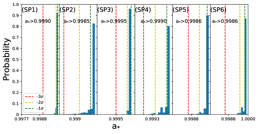
Figure 2: Histograms of $a_{*}$ calculated via the Monte Carlo analysis for 3000 sets of parameters per spectrum. The three dashed lines from left to right imply the 99.7% (3$\sigma$, red), 95.4% (2$\sigma$, yellow), and 68.3% (1$\sigma$, green) error, respectively. The respective 99.7% confidence lower limit on $a_{*}$ is indicated in each panel.

Three typical components might be included in the spectrum of a black hole X-ray binary, namely the thermal, power-law and reflection components (refer to Figure 2 in GOU11 for a schematic illustration of these different components).

The model we employed in this paper is the most advanced and physically realistic model used in GOU11 and GOU14. The structure of the model, naming all the components that it comprises, with a concise description of each one, are as follows (the detailed parameter configuration is the same as GOU11 and GOU14, unless otherwise indicated):

$${\rm CRABCOR*CONSTANT*TBABS~{}[SIMPLR\otimes KERRBB{\small 2}+KERRDISK+~{}KERRCONV\otimes(IREFLECT\otimes SIMPLC)]}$$

Thermal component: The thermal radiation is emitted from the accretion disk. kerrbb2 (McClintock et al., 2006) is a fully relativistic thin disk model, including the effects of the returning radiation and the limb darkening. This model reads in and uses a pair of look-up tables for the spectral hardening factor $f$, computed using bhspec (Davis et al. 2005, Davis & Hubeny 2006) and kerrbb (Li et al. 2005), corresponding to two representative values of the viscosity parameter: $\alpha$ = 0.01 and $\alpha$ = 0.1 (here we adopt $\alpha$ = 0.1). kerrbb2 only has two principal fit parameters: the dimensionless spin parameter a_∗, and the mass accretion rate $\dot{M}$.

Power-law Component: The thermal seed photons supplied by the accretion disk are inverse-Compton scattered into the power-law component by hot electrons in the corona. The convolution model simplr, a modified version of simpl (Steiner et al. 2009a), is an advanced empirical Comptonization model including three main fit parameters: the photon power-law index $\Gamma$, the scattered fraction $f_{\rm sc}$ and the reflection constant parameter $\chi$. As we mentioned, we adopt f${}_{\rm sc}\lesssim 25\%$ as our spectrum selection standard.

Reflection Component: A fraction of the scattered seed photons are emitted downward toward the disk, illuminating the disk and generating the reflection component. kerrdisk + kerrconv$\otimes$ (ireflect $\otimes$ simplc)] models the entire reflection component including the Compton hump, the absorption edge and the emission lines. simplc represents the part of the power-law component that strikes the disk (Steiner et al. 2009a), which is regarded as the input spectrum for the convolution model ireflect (Magdziarz & Zdziarski 1995). Photons emitted near the black hole suffer various relativistic effects, leading to a blurring of the observed spectrum. kerrconv is utilized with the aim of smearing the spectrum (Brenneman & Reynolds, 2006). kerrdisk is a model for the iron emission line with the spin allowed to be a free parameter (Brenneman & Reynolds, 2006). Here it should be noted that the effect on the spin measurements of using different reflection models is almost negligible, as demonstrated in section 5.3 of GOU11.

In addition, we use three multiplicative models: (1) crabcor is used for correcting calibration deviations of RXTE. (2) constant is an energy-independent multiplicative factor in order to reconcile calibration discrepancies between different detectors. (3) tbabs is an ISM absorption model (Wilms et al. 2000).

3.2 Fit Results

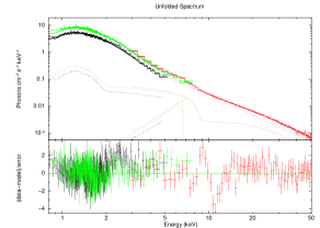
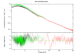
Figure 1: A representative best-fit X-ray spectrum (SP3). Left: A plot of the unfolded spectrum and the model. Right: A plot of the spectrum with the folded model. Detailed fit parameters are listed in Table 2. The data obtained by RXTE is plotted in red. For the Chandra observation we used, the data collected by the High Energy Grating (HEG) and Medium Energy Grating (MEG) components of the High-Energy Transmission Grating (HETG) are plotted as green and black, respectively. The dotted lines represent the models we adopted.

Our model provides a good fit to all six spectra, with reduced $\chi^{2}$ values varying from 1.12 to 1.49. The fit parameters are shown in Table 2. A representative plot of the unfolded spectrum is given in Figure 1. It is noticed that there is a larger residual between 8 keV and 15 keV, which will be discussed in detail later, and should not significantly affect the spin results.

As a caveat, in all six cases, the values of $a_{*}$ reached the maximum value of the XSPEC model kerrbb2, 0.9999. This value is larger than the physical upper limit of a_∗, which we will discuss in the next section. The preliminary error in $a_{*}$ computed with XSPEC and listed in Table 2 is due to counting statistics, while the final adopted error due to the combined uncertainties in $D$, $M$, and $i$ is acquired via our Monte Carlo analysis.

Requiring the spectrum to be dominated by accretion disk component for reliable application of the continuum-fitting method, we adopt $f_{\rm sc}\lesssim 25\%$ as the selection standard. The values of this parameter in our analysis, 24.7% $\pm$ 0.5%, 10.6% $\pm$ 1.6%, 15.6% $\pm$ 1.2%, 21.1% $\pm$ 1.0%, 16.3% $\pm$ 0.9%, 9.3% $\pm$ 0.2%, satisfy this standard.

It is equally essential to select spectra with bolometric Eddington-scaled luminosities $l<0.3$ (McClintock et al. 2006, Zhu et al. 2012, McClintock et al. 2014), in order to ensure a geometrically thin disk. This parameter is quite stable and low in our analysis, ranging from 0.01 to 0.03, which meets this criteria without difficulty.

3.3 Error Analysis

Previous work on estimating $a_{*}$ had found that the combined observational uncertainties in $M$, $i$ and $D$ dominate the error budget (GOU11, McClintock et al. 2014). This part of the error is usually calculated through Monte Carlo simulations (Liu et al. 2008, Gou et al. 2011, McClintock et al. 2014). In order to do so, for each individual spectrum, the procedure is as follows: (1) Assuming that each one of these three parameters is independent and Gaussian distributed, we generate 3000 sets of ($M$, $i$, $D$). (2) Then we calculate look-up tables of $f$ for these parameter sets. (3) Finally we fit the spectrum to our adopted model to determine $a_{*}$. With 3000 simulations run, we obtain the histogram of $a_{*}$.

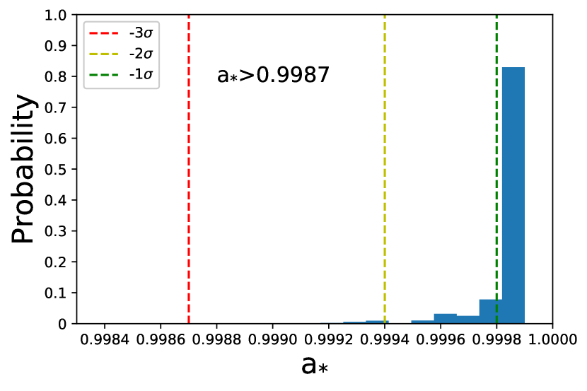
Figure 3: Summed histogram of $a_{*}$ for our six spectra, including 18000 data points. The dashed lines and listed 99.7% confidence lower limit in this figure are as those shown in Figure 2.

After repeating the procedure expressed above for all six spectra, we obtain six histograms of $a_{*}$. The histogram for each spectrum is shown in Figure 2, and the summed histogram is plotted in Figure 3. The spin value in SP2 is lowest, therefore we report the final result of $a_{*}>0.9985$ $(3\sigma)$ based on a conservative estimation from this spectrum.

4 discussion

4.1 Comparison with the Thorne Limit

In this paper, we have obtained a much more stringent limit on the spin of the black hole in Cygnus X-1 than found from previous work: $a_{*}>0.9985$ at 3$\sigma$ level of confidence. This very high spin parameter confirms that Cygnus X-1 hosts an extreme Kerr black hole.

However, Thorne (1974) pointed out that the maximum expected spin once the absorption of hot photons from the disk is taken into account is 0.998 (hereafter, the Thorne limit), as the absorption will produce an counteracting torque when the spin is extremely high. We note that our spin constraint is slightly higher than the Thorne limit. This is mainly because the upper limit in our model kerrbb2 is set at 0.9999, and our obtained spin parameter is based purely on the theoretical model.

It should be noted that although the Thorne limit has generally been adopted by the community as a reasonable guess for an astrophysical upper limit, there is still some debate as to the exact value of the upper limit. Sadowski et al. (2011) suggested that black holes with super-critical accretion flows could reach an equilibrium spin value up to 0.9994, which exceeds the Thorne limit. They showed that the equilibrium spin value depends strongly on the assumed value of the viscosity parameter, and also proved that for high accretion rates the impact of captured radiation on spin evolution is negligible. Cygnus X-1 is not believed to be in the super-critical regime, and hence these considerations may not apply. However, a number of other factors might affect the precise spin measurement, and they are discussed in the following sections. Regardless, the spin of Cygnus X-1 appears to be very high, as found previously by both continuum fitting (GOU11, GOU14) and iron line fitting studies (Fabian et al. 2012, Tomsick et al. 2014, Parker et al. 2015, Duro et al. 2016, Walton et al. 2016, Tomsick et al. 2018).

4.2 Effect of a Possible Spin-orbit Misalignment

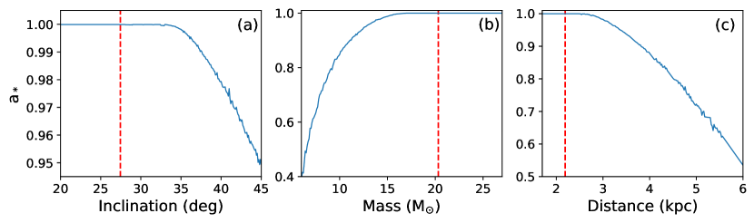
Figure 4: Effects on $a_{*}$ of varying one of the three input parameters while fixing the other two at their updated values. (a) Spin vs. inclination angle $i$; (b) spin vs. black hole mass $M$; (c) spin vs. source distance $D$. The red dashed lines represent the baseline values $i$ = 27.51 ^∘, $M$ = 21.2 and $D$ = 2.22 kpc. These plots were made using the fit results of SP6.

Figure 4 shows the effect on $a_{*}$ of separately varying the input parameters $M$, $i$, and $D$. $a_{*}$ takes the extreme value of 0.9999 when all three parameters are fixed on their newly-obtained, best-fitting values.

In applying the continuum-fitting method, we assume that the binary orbital angular momentum vector is aligned with the spin axis of the black hole. Cygnus X-1 is suggested to have formed with little to no natal kick (Mirabel & Rodrigues 2003, Rao et al. 2019), so the spin axis of the black hole should still be aligned with the orbital angular momentum vector (as discussed by Miller-Jones et al. (2020), who estimated a likely maximum misalignment angle of order $10^{\circ}$).

However, there is still controversy about this assumption. Some previous work on fitting the reflection component of Cygnus X-1 suggested a different inner disk inclination angle compared to the binary orbital inclination, which implies a possible spin-orbit misalignment (also suggested in some other black hole binary systems, Fragos et al. 2010, Dong et al. 2020). Tomsick et al. (2014) evaluated the lower limit of this misalignment to be $13^{\circ}$. Walton et al. (2016) estimated the magnitude of a disk warp to be about $10^{\circ}-15^{\circ}$. However, these fits often require very high iron abundances, and Tomsick et al. (2018) recently found that a much lower disk inclination of $<$ 20^∘ could be accommodated if the electron density was free to vary, even suggesting that a misalignment might not even be required in this scenario. Thus, while the possibility of a misalignment should be considered, this scenario would appear to remain under debate.

Nonetheless, we investigated this possibility, and as shown in Figure 4(a), the value of $a_{*}$ monotonically decreases with increasing $i$. We find that even given a misalignment angle of $15^{\circ}$ (equivalent to $i$ = $42.47^{\circ}$), the spin value is 0.9696 (see Case 1 in Table 2), which is still very high.

4.3 Effect of the Metallicity

The spectral hardening factor $f$ in kerrbb2 is pre-calculated with a table model bhspec, which is related to the metallicity $Z$. Our fit results are all given for $Z$ = 1 $Z_{\odot}$. However, the metallicity of Cygnus X-1 is slightly super-solar (Shimanskii et al. 2012), as also implied by the fitted super-solar values of Fe abundance in our reflection model ireflect.

Unfortunately, the current model bhspec only contains two possible metallicity cases ($Z$ = 1 $Z_{\odot}$ and $Z$ = 0.1 Z_⊙), and does not yet have an option for super-solar abundance. However, if the metallicity increases, the value of the spin increases slightly. In addition, substantial changes in metallicity only produce a negligible effect on spin. For example, as stated in Gou et al. 2009, the spin of the black hole in LMC X-1 increases from 0.937 $\pm$ 0.020 to 0.938 $\pm$ 0.020 if Z increases from 0.1 Z_⊙ to 1 Z_⊙.

4.4 Effect of the Viscosity Parameter

Throughout this work, in order to get a more conservative constraint, we fixed the viscosity parameter $\alpha$ to 0.1, because $a_{*}$ increases slightly as $\alpha$ decreases (Gou et al. 2009). However, we reanalyzed our data using $\alpha$ = 0.01, and found that the results remain unchanged, as they have already reached their maximum value of 0.9999.

4.5 Effect of a Finite Disk Height

The model utilized in the continuum-fitting method is the general relativistic Novikov-Thorne model that assumes a razor-thin disk. However, a real accretion disk will have finite thickness, which will affect measurements of the black hole spin. Kulkarni et al. (2011) evaluated the error introduced by the deviations from the Novikov-Thorne model. They computed disk spectra obtained from three-dimensional general relativistic magnetohydrodynamic (GRMHD) simulations, and then fitted these simulated spectra with kerrbb. By comparing the spin results with the spin used in the GRMHD simulations, they concluded that the model errors become obvious only at low spins and high inclinations. In the case of $i$ = 30^∘ and a_∗ = 0.98 (close to the values estimated for Cygnus X-1), the spin calculated by fitting the simulated spectra was 0.985 $\pm$ 0.001 and the value of $\triangle$ $a_{*}$ is 0.005. Moreover, they might have overestimated the error due to the deviation from the Novikov-Thorne model because their simulation results are for a thicker disk with a bolometric Eddington-scaled luminosity $l$ = 0.4–0.7, while the bolometric Eddington-scaled luminosity of Cygnus X-1 in this paper is only 0.02 (as stated in Section 6 of GOU11).

4.6 The Residual Structure between 8–15 keV

We notice that there is a larger residual between 8 keV and 15 keV, which is not fitted with the current model. However, it should be emphasized that the spin parameter is determined from the disk thermal component (which dominates the spectra, peaks around 1.5 keV, and is concentrated below 6 keV; see Figure 3 of GOU11 for reference), and thus the residual between 8 and 15 keV should not significantly affect the spin results.

Previous work has proposed many theories to explain similar residual structures. Fabian et al. (2020) found an 7–9 keV excess emission component during the soft state in spectra of MAXI J1820+070. They explained this additional component by including another blackbody whose temperature is slightly higher than that of the disk itself. Given that the higher temperature, the additional emission is linked to the innermost region of the disk and with the start of the plunging region. In this region, the density is still high enough to heat the gas, possibly emitting blackbody radiation. We utilized an addition model BBODY to describe this component, we find that the fit is poor ($>2$), and the spin could not be determined certainly.

Another possibility is that the observed residual structure is an additional Comptonization component. In our fits, we only utilized Comptonization models which have a pure non-thermal power-law electron distribution. However, some previous work of the fast time variability seen in the high/soft state prefer a stratified Comptonization spectrum (Grinberg et al. 2014). It is likely that there exist hybrid thermal/non-thermal electron distributions, resulting in an additional low temperature thermal comptonization component (Gierli+etal+1999, Zdziarski et al. 2002, Kawano et al. 2017). This component then produce a higher energy power-law tail, which would also lead us to overestimate the black hole spin. For instance, as mentioned in Kawano et al. (2017), the spin of the black hole in Cygnus X-1 is 0.95 $\pm$ 0.01 for a simple non-thermal Comptonization; and decreases to 0.80 ${}^{+0.08}_{-0.30}$ for hybrid thermal/non-thermal Comptonization. A similar residual structure between 5–10 keV was found in the spectra of the black hole candidate MAXI J1828-249 in a possible intermediate state (Oda et al. 2019). They modeled this excess with a Comptonization of disk photons by thermal electrons with a relatively low temperature and inferred it could be generated in a region where the disk inner edge intrudes into the hot inner flow, or a Comptonizing region above the disk surface. We used an addition model comptt to describe the Comptonization of soft photons, and reflected both two Comptonization components. The model is reconstructed as follows:

$${\rm CRABCOR*CONSTANT*TBABS~{}[KERRBB{\small 2}+SIMPL\otimes COMPTT}$$

$${\rm+KERRDISK+~{}KERRCONV\otimes(IREFLECT\otimes SIMPL\otimes COMPTT)]}$$

The fit parameters are listed in Table 3. For SP1, the fit is better than former model with reduced $\chi^{2}$ reducing from 1.49 to 0.94. The spin parameter $a_{*}$ decreases from 0.9999 to $0.9947\pm 0.0014$. The photon power-law index decreases from $2.39\pm 0.01$ to $1.99\pm 0.01$. The scattered fraction $f_{\rm sc}$ is larger ranging from $0.247\pm 0.005$ to $0.399\pm 0.007$. For SP2-SP6, the values of $a_{*}$ are unaffected, which are still at 0.9999. However, the errors quoted here (estimated in XSPEC) are obviously larger. Besides, for these five spectra, this model can’t constrain the parameters of comptt well probably because the component is weak. The scattered fraction $f_{\rm sc}$ are somehow increasing from $\sim 0.15$ to $\sim 0.40$. For SP5, the fit is slightly worse with reduced $\chi^{2}$ increasing from 1.25 to 1.27. While for SP2, SP3, SP4 and SP6, the fit is better with reduced $\chi^{2}$ ranging from 1.12, 1.15, 1.32, 1.24 to 0.93, 1.02, 0.94, 1.12, respectively. We also try the same setup of Kawano et al. (2017), fixing $T_{\rm 0}$, $kT$ and $\tau$ at 0.44 keV, 3.4 keV and 1.66, respectively. Details are shown in Case 1 of Table 3. The spin parameter $a_{*}$ is still pegged at 0.9999.

Whether using a hybrid thermal/non-thermal Comptonization model or a single non-thermal Comptonization model, we all get an extremely high spin. So we can conclude that including comptt is not having the same effect as in Kawano et al. (2017). However, it is interesting to note that the reduced $\chi^{2}$ decreases significantly (e.g., for SP1 it goes to 0.94 from 1.49), which means that adding this Comptonization model is having a large impact on the high energy Compton component rather than on the disk which is the foundation of our spin measurements.

4.7 Comparison with the Reflection Measurements

Another widely-used technique of measuring the spin is the iron-line profile fitting method (Fabian et al. 1989, Reynolds & Nowak 2003). As mentioned above, some portion of the power-law component is reflected by the disk, generating the reflection spectrum whose main prominent features include the fluorescent emission lines (in particularly, the iron K$\alpha$ line between 6.4 - 6.97 keV, depending on ionization state) and the Compton hump at 20 - 30 keV (Ross et al. 1999). The intrinsically narrow iron K$\alpha$ line is then broadened and smeared by the combined effects of Doppler shift, special relativity, and general relativity (Fabian et al. 2000), and by fitting the iron-line profile, one can deduce the spin parameter.

The spin results from the continuum-fitting method both in the previous work and in this work are consistent with the spins derived from the reflection method (Duro et al. 2011, Fabian et al. 2012, Tomsick et al. 2014, Parker et al. 2015, Duro et al. 2016, Walton et al. 2016, Tomsick et al. 2018), although Miller et al. (2002) found a near-zero spin of Cygnus X-1, which is mainly because the lack of adequate energy coverage ($\lesssim$ 10 keV) made it difficult to subtract the underlying continuum properly.

It should be noted that the highly-sensitive NuSTAR, launched in 2012, provides unprecedentedly precise measurements of the iron line region and reflection component. In the soft state, Tomsick et al. (2014) reported a rapid spin of $a_{*}$ $>$ 0.83 and Walton et al. (2016) estimated a higher spin of 0.93 $\lesssim a_{*}\lesssim$ 0.96. Parker et al. (2015) analyzed observations taken in the hard state and found a high spin of $a_{*}$ $>$ 0.97. In the intermediate state, Tomsick et al. (2018) restricted the spin to be $a_{*}>0.93$ for the high-density reflection model.

In addition, Duro et al. (2016) analyzed a spectra of four simultaneous hard intermediate state observations, and found a spin of $\simeq$ 0.9. They also suggested that the different inclination angles inferred in the different states (i.e., the reported inclination angle of $\simeq$ 30^∘ in the hard intermediate state, as compared to the higher inclinations found from the reflection measurements in the soft state) could imply a warp in the inner region of the disk. However, as discussed by Tomsick et al. (2018), these results can be somewhat degenerate with the iron abundance and with the disk electron density.

4.8 Spin Comparison with Other Systems

We found that the spin of Cygnus X-1 is constrained to be $a_{*}>0.9985$, which is the highest among all the stellar-mass black hole systems with a measured spin parameter. Although it may be less extreme due to some systematics, this value would be still very high. If we look through the spin parameters measured for the stellar-mass black hole systems using the continuum-fitting method, it shows that almost all the black holes in high-mass X-ray binaries have a relatively high spin (Cygnus X-1: $a_{*}>0.9985$, this work; LMC X-1: $a_{*}=0.92^{+0.05}_{-0.07}$, Gou et al. 2009; M33 X-7: $a_{*}=0.84\pm 0.05$, Liu et al. 2010; IC10 X-1: $a_{*}\gtrsim 0.8$, Steiner et al. 2016). However, the low mass X-ray binaries have a wide range of spins between zero and unity, which may imply different evolutionary paths for these systems (Bambi 2019, Reynolds 2019).

It is noted that, since the first detection of GW150914 in 2015, LIGO and Virgo have made 3 runs, and also made 50 detections of gravitational wave events with majority of stellar mass binary black hole systems. The results from the first 2 runs have been catalogued in Abbott et al. (2019), which shows the effective spin $\chi_{\rm eff}$ of the binary system before merger is quite small with the distribution’s mean $\mu\approx 0$, and with a narrow distribution, which is confirmed by Miller et al. (2020). Miller et al. (2020) further explored what these ensemble properties imply about the spins of individual binary black hole mergers, re-analyzing existing gravitational-wave events with a population-informed prior on their effective spin, and found, under this analysis, the binary black hole GW170729, which previously excluded $\chi_{\rm eff}$ = 0, is now consistent with zero effective spin at $\approx 10\%$ credibility.

As we know, the companion star of Cygnus X-1 is around 40 $M_{\odot}$, and based on our understanding to the stellar evolution, it may eventually produce a second black hole of the system, forming a binary black hole system in the future. In addition, the current analysis to the system shows that the black hole spin-orbit misalignment is small, within 10 degree (Miller-Jones et al. 2020). If the black hole of Cygnus X-1 and the companion star were formed from the same cloud initially, then the companion star is usually aligned with the orbital plane. In this case, we should expect the effective spin of the system is quite large, unless there is a large asymmetric kick during the black hole formation of the companion star, and it will be quite different from the spin distribution obtained from the GW results. This may imply that Cygnus X-1 system is likely to follow a different formation channel (primordial one) compared to the GW black hole system, although it is not clear whether the GW results preferentially support a dynamical or field binary origin (or even other possibilities) for stellar mass binary black holes detected by GWs. Furthermore, Miller-Jones et al. (2020) shows that, given the current orbital separation, we do not expect Cygnus X-1 or systems with similar properties to yield binary black hole mergers in the age of the Universe. So we may haven’t detect any GW signal from primordial binary black hole systems yet.

As to the origin of the high spin in these high-mass systems, it is usually concluded that the spin is natal (Podsiadlowski et al. 2003, Axelsson et al. 2011, Qin et al. 2019), at least for those high-mass X-ray binaries, mainly because in the whole lifetime of a stellar-mass black hole, it is centainly impossible to spin up from zero to a highly-spinning black hole via standard (as opposed to hypercritical) accretion (Wong et al. 2012). One possible evolutionary channel to explain the high spin is that the BH progenitor undergoes mass transfers while still in the main sequence (see Case-A MT in Qin et al. 2019). Hence the core of the BH progenitor contains enough angular momentum to form a highly rotating black hole (many observational features predicted by this path, such as unusual surface abundances of the secondary, have been found in Cygnus X-1, as mentioned in Miller-Jones et al. 2020).

5 conclusion

We re-analyze six archival spectra of the black hole X-ray binary Cygnus X-1, which were originally presented in GOU11 and GOU14, to constrain the black hole spin. We adopt up-to-date values of three key dynamical parameters $M$, $i$, and $D$. These data rigorously satisfy the selection criterion f${}_{\rm sc}\lesssim 25\%$. The key model we utilized is a fully relativistic thin disk model kerrbb2. Monte Carlo simulations are performed in order to estimate the error in $a_{*}$ due to the combined uncertainties of $M$, $i$, and $D$. Ultimately, we arrive at our final result, $a_{*}>0.9985$ at the 3$\sigma$ level of confidence, which confirms the extreme spin of the black hole in Cygnus X-1.

It should be noted that the spin value we presented above is the theoretical one purely based on the model itself, and the hard limit is set at 0.9999. In practice, the maximum spin value could be slightly lower than 0.9999. Thorne (1974) estimated the evolution of a black hole, and pointed out that the maximum spin of a black hole can only reach 0.998 because the radiation from the accretion disk will produce a counteracting torque on the black hole once the black hole reaches the maximum spin. Given the Thorne limit, we conclude that the black hole in Cygnus X-1 has an extreme spin in any event.

Table 1: Log of the Observations^a

Number	ObsID	Mission	Detector	Energy Band (keV)	UT	Texp (s)	I (Crab)	$\phi$
SP1	10408000 $\&$ P10412	ASCA $\&$ RXTE	GIS $\&$ PCA	0.7–8.0 $\&$ 2.5–45.0	1996-05-30 06:43:16 $\&$ 07:51:29	2547 $\&$ 2240	0.80	0.74
SP2	12472 $\&$ P96378	Chandra $\&$ RXTE	HETG(CC) $\&$ PCA	0.8–8.0 $\&$ 2.9–50	2011-01-06 14:06:40–14:35:44	455 $\&$ 1744	0.52	0.32
SP3	12472 $\&$ P96378	Chandra $\&$ RXTE	HETG(CC) $\&$ PCA	0.8–8.0 $\&$ 2.9–50	2011-01-06 15:44:16–16:09:52	398 $\&$ 1536	0.61	0.33
SP4	12472 $\&$ P96378	Chandra $\&$ RXTE	HETG(CC) $\&$ PCA	0.8–8.0 $\&$ 2.9–50	2011-01-06 17:15:28–17:43:44	455 $\&$ 1744	0.57	0.35
SP5	12472 $\&$ P96378	Chandra $\&$ RXTE	HETG(CC) $\&$ PCA	0.8–8.0 $\&$ 2.9–50	2011-01-06 18:19:44–19:17:52	455 $\&$ 1744	0.38	0.36
SP6	12472 $\&$ P96378	Chandra $\&$ RXTE	HETG(CC) $\&$ PCA	0.8–8.0 $\&$ 2.9–50	2011-01-06 19:53:36–20:50:08	455 $\&$ 1744	0.38	0.37

Table 2: Best-fit Results for Our Adopted Model^a

Number	Model	Parametera	Spectral Number						Case 1b
			SP1	SP2	SP3	SP4	SP5	SP6
1	tbabs	$N_{\rm H}$	0.74 $\pm$ 0.01	0.82 $\pm$ 0.02	0.83 $\pm$ 0.03	0.80 $\pm$ 0.02	0.79 $\pm$ 0.02	0.81 $\pm$ 0.01	0.72 $\pm$ 0.01
2	simplr	$\Gamma$	2.39 $\pm$ 0.01	2.38 $\pm$ 0.04	2.46 $\pm$ 0.03	2.69 $\pm$ 0.02	2.62 $\pm$ 0.03	2.50 $\pm$ 0.01	2.45 $\pm$ 0.01
3	simplr	$f_{\rm sc}$	0.247 $\pm$ 0.005	0.106 $\pm$ 0.016	0.156 $\pm$ 0.012	0.211 $\pm$ 0.010	0.163 $\pm$ 0.009	0.093 $\pm$ 0.002	0.092 $\pm$ 0.002
4	kerrbb2	$a_{*}$	$0.9999^{+0.0000}_{-0.0087}$	$0.9999^{+0.0000}_{-0.0137}$	$0.9999^{+0.0000}_{-0.0155}$	$0.9999^{+0.0000}_{-0.0130}$	$0.9999^{+0.0000}_{-0.0115}$	$0.9999^{+0.0000}_{-0.0015}$	$0.9696\pm 0.0034$
5	kerrbb2	$\dot{M}$	0.17 $\pm$ 0.02	0.20 $\pm$ 0.03	0.19 $\pm$ 0.04	0.19 $\pm$ 0.03	0.18 $\pm$ 0.03	0.18 $\pm$ 0.01	0.23 $\pm$ 0.01
6	kerrdisk	$E_{\rm L}$	6.57 $\pm$ 0.06	6.74 $\pm$ 0.08	6.55 $\pm$ 0.07	6.40 $\pm$ 0.13	6.55 $\pm$ 0.11	6.70 $\pm$ 0.08	6.46 $\pm$ 0.06
7	kerrdisk	$q$	2.89 $\pm$ 0.08	3.00 $\pm$ 0.09	2.73 $\pm$ 0.11	1.64 $\pm$ 0.40	2.66 $\pm$ 0.17	2.95 $\pm$ 0.06	3.45 $\pm$ 0.10
8	kerrdisk	$N_{\rm L}$	0.009 $\pm$ 0.001	0.024 $\pm$ 0.003	0.029 $\pm$ 0.003	0.012 $\pm$ 0.002	0.011 $\pm$ 0.002	0.014 $\pm$ 0.001	0.026 $\pm$ 0.001
9	kerrdisk	EW	0.11	0.36	0.29	0.14	0.21	0.29	0.61
10	ireflect	$X_{\rm Fe}$	6.3 $\pm$ 0.3	6.0 $\pm$ 1.1	3.9 $\pm$ 0.5	3.5 $\pm$ 0.3	5.9 $\pm$ 0.6	4.1 $\pm$ 0.6	3.5 $\pm$ 0.6
11	ireflect	$\xi$	62 $\pm$ 10	335 $\pm$ 186	137 $\pm$ 45	21 $\pm$ 7	57 $\pm$ 18	381 $\pm$ 51	412 $\pm$ 64
12	constant	$N_{\rm ASCA}$	0.955 $\pm$ 0.003	-	-	-	-	-	-
13	constant	$N_{\rm MEG}$	-	0.688 $\pm$ 0.009	0.575 $\pm$ 0.007	0.704 $\pm$ 0.007	0.713 $\pm$ 0.005	0.682 $\pm$ 0.006	0.690 $\pm$ 0.011
14	constant	$N_{\rm HEG}$	-	0.863 $\pm$ 0.011	0.889 $\pm$ 0.012	0.887 $\pm$ 0.009	0.923 $\pm$ 0.007	0.889 $\pm$ 0.008	0.903 $\pm$ 0.014
15		Reduced $\chi^{2}$ ($\chi^{2}$/degree)	1.49 (678.09/454)	1.12 (705.15/627)	1.15 (656.82/572)	1.32 (823.61/624)	1.25 (929.81/744)	1.24 (1241.40/998)	1.09 (1087.79/998)
16		$f$	1.6	1.6	1.6	1.6	1.6	1.6	1.5
17		$l$	0.02	0.03	0.03	0.02	0.02	0.02	0.02

Table 3: Best-fit Results for a Hybrid Thermal/Non-thermal Comptonization Model

Number	Model	Parameter	Spectral Number						Case 1b
			SP1	SP2	SP3	SP4	SP5	SP6
1	tbabs	$N_{\rm H}$	0.73$\pm$0.01	0.73 $\pm$ 0.05	0.71 $\pm$ 0.06	0.65 $\pm$ 0.06	0.71 $\pm$ 0.03	0.75 $\pm$ 0.04	0.76 $\pm$ 0.02
2	kerrbb2	$a_{*}$	0.9947 $\pm$ 0.0014	$0.9999^{+0.0000}_{-0.1587}$	$0.9999^{+0.0000}_{-0.2105}$	$0.9999^{+0.0000}_{-0.1798}$	$0.9999^{+0.0000}_{-0.0903}$	$0.9999^{+0.0000}_{-0.1449}$	$0.9999^{+0.0000}_{-0.0169}$
3	kerrbb2	$\dot{M}$	0.18 $\pm$ 0.01	0.14 $\pm$ 0.06	0.22 $\pm$ 0.02	0.25 $\pm$ 0.03	0.13 $\pm$ 0.10	0.29 $\pm$ 0.05	0.16 $\pm$ 0.03
4	simplr	$\Gamma$	1.99 $\pm$ 0.01	2.40 $\pm$ 0.04	2.46 $\pm$ 0.02	2.53 $\pm$ 0.02	2.43 $\pm$ 0.05	2.52 $\pm$ 0.02	2.39 $\pm$ 0.02
5	simplr	$f_{\rm sc}$	0.399 $\pm$ 0.007	0.447 $\pm$ 0.440	0.431 $\pm$ 0.359	0.393 $\pm$ 0.198	0.361 $\pm$ 0.234	0.361 $\pm$ 0.311	0.492 $\pm$ 0.176
6	comptt	$T_{\rm 0}$ a	0.45$\pm$0.06	0.45 $\pm$ 0.44	0.40 $\pm$ 0.23	0.41 $\pm$ 0.36	0.39 $\pm$ 0.16	0.42 $\pm$ 0.26	0.44(fixed)
7	comptt	$kT$ a	5.77$\pm$2.51	$3.87^{+125.44}_{-3.77}$	$4.00^{+113.39}_{-3.90}$	$4.11^{+164.92}_{-4.01}$	$4.06^{+96.8}_{-3.96}$	$3.95^{+109.05}_{-3.85}$	3.4(fixed)
8	comptt	$\tau$ a	2.08$\pm$0.74	$0.81^{+37.60}_{-0.80}$	$0.63^{+26.64}_{-0.62}$	$0.33^{+23.50}_{-0.32}$	$0.80^{+26.65}_{-0.79}$	$0.43^{+19.5}_{-0.42}$	1.66(fixed)
9	comptt	$\rm Norm$ a	1.08$\pm$0.48	$2.50^{+88.45}_{-2.50}$	$3.64^{+110.73}_{-3.64}$	$3.86^{+165.12}_{-3.86}$	$2.15^{+55.37}_{-2.15}$	$2.41^{+70.82}_{-2.41}$	2.12$\pm$ 0.07
10	kerrdisk	$E_{\rm L}$	6.59$\pm$0.04	6.56 $\pm$ 0.07	6.51 $\pm$ 0.08	6.49 $\pm$ 0.08	6.57 $\pm$ 0.07	6.55 $\pm$ 0.08	6.54 $\pm$ 0.07
11	kerrdisk	$q$	2.74$\pm$0.03	2.51 $\pm$ 0.19	2.50 $\pm$ 0.21	2.52 $\pm$ 0.22	2.53 $\pm$ 0.19	2.57 $\pm$ 0.19	2.38 $\pm$ 0.16
12	kerrdisk	$N_{\rm L}$	0.019$\pm$0.001	0.020 $\pm$ 0.004	0.023 $\pm$ 0.004	0.020 $\pm$ 0.004	0.014 $\pm$ 0.003	0.013 $\pm$ 0.002	0.019 $\pm$ 0.002
13	kerrdisk	EW	0.21	0.29	0.25	0.23	0.29	0.26	0.26
14	ireflect	$X_{\rm Fe}$	2.2$\pm$0.1	5.3 $\pm$ 1.2	3.8 $\pm$ 0.6	4.5 $\pm$ 0.8	4.1 $\pm$ 1.0	3.9 $\pm$ 0.8	4.4 $\pm$ 0.5
15	ireflect	$\xi$	198$\pm$11	107 $\pm$ 48	80 $\pm$ 31	92 $\pm$ 37	111 $\pm$ 48	128 $\pm$ 53	89 $\pm$ 19
16	constant	$N_{\rm ASCA}$	1.012$\pm$0.003	-	-	-	-	-	-
17	constant	$N_{\rm MEG}$	-	0.824 $\pm$ 0.010	0.664 $\pm$ 0.008	0.813 $\pm$ 0.009	0.803 $\pm$ 0.007	0.800 $\pm$ 0.008	0.820 $\pm$ 0.009
18	constant	$N_{\rm HEG}$	-	1.037 $\pm$ 0.012	1.029 $\pm$ 0.012	1.026 $\pm$ 0.012	1.039 $\pm$ 0.009	1.045 $\pm$ 0.010	1.031 $\pm$ 0.011
19		Reduced $\chi^{2}$ ($\chi^{2}$/degree)	0.94 (430.62/451)	0.93 (581.00/624)	1.02 (580.58/572)	0.94 (582.79/621)	1.27 (941.07/741)	1.12 (1114.26/994)	0.93 (583.43/627)
20		$f$	1.6	1.6	1.5	1.6	1.6	1.6	1.6
21		$l$	0.02	0.02	0.01	0.02	0.02	0.02	0.02

References

- Abbott et al. (2019) Abbott, B. P., Abbott, R., Abbott, T. D., et al. 2019, Physical Review X, 9, 031040
- Axelsson et al. (2011) Axelsson, M., Church, R. P., Davies, M. B., et al. 2011, MNRAS, 412, 2260
- Bambi (2019) Bambi, C. 2019, arXiv e-prints, arXiv:1906.03871
- Bardeen et al. (1972) Bardeen, J. M., Press, W. H., & Teukolsky, S. A. 1972, ApJ, 178, 347
- Brenneman & Reynolds (2006) Brenneman, L. W., & Reynolds, C. S. 2006, ApJ, 652, 1028
- Chen et al. (2016) Chen, Z., Gou, L., McClintock, J. E., et al. 2016, ApJ, 825, 45
- Davis et al. (2005) Davis, S. W., Blaes, O. M., Hubeny, I., et al. 2005, ApJ, 621, 372
- Davis & Hubeny (2006) Davis, S. W., & Hubeny, I. 2006, ApJS, 164, 530
- Dong et al. (2020) Dong, Y., García, J. A., Steiner, J., et al. 2020, MNRAS, 493, 4409
- Duro et al. (2011) Duro, R., Dauser, T., Wilms, J., et al. 2011, A&A, 533, L3
- Duro et al. (2016) Duro, R., Dauser, T., Grinberg, V., et al. 2016, A&A, 589, A14
- Fabian et al. (1989) Fabian, A. C., Rees, M. J., Stella, L., et al. 1989, MNRAS, 238, 729
- Fabian et al. (2000) Fabian, A. C., Iwasawa, K., Reynolds, C. S., et al. 2000, PASP, 112, 1145
- Fabian et al. (2012) Fabian, A. C., Wilkins, D. R., Miller, J. M., et al. 2012, MNRAS, 424, 217
- Fragos et al. (2010) Fragos, T., Tremmel, M., Rantsiou, E., et al. 2010, ApJ, 719, L79
- Fabian et al. (2020) Fabian, A. C., Buisson, D. J., Kosec, P., et al. 2020, MNRAS, 493, 5389
- García et al. (2014) García, J. A., McClintock, J. E., Steiner, J. F., et al. 2014, ApJ, 794, 73
- García et al. (2016) García, J. A., Grinberg, V., Steiner, J. F., et al. 2016, ApJ, 819, 76
- Gou et al. (2009) Gou, L., McClintock, J. E., Liu, J., et al. 2009, ApJ, 701, 1076
- Gou et al. (2010) Gou, L., McClintock, J. E., Steiner, J. F., et al. 2010, ApJ, 718, L122
- Gou et al. (2011) Gou, L., McClintock, J. E., Reid, M. J., et al. 2011, ApJ, 742, 85
- Gou et al. (2014) Gou, L., McClintock, J. E., Remillard, R. A., et al. 2014, ApJ, 790, 29
- Grinberg et al. (2014) Grinberg, V., Pottschmidt, K., Böck, M., et al. 2014, A&A, 565, A1
- Kawano et al. (2017) Kawano, T., Done, C., Yamada, S., et al. 2017, PASJ, 69, 36
- Kolehmainen & Done (2010) Kolehmainen, M., & Done, C. 2010, MNRAS, 406, 2206
- Kulkarni et al. (2011) Kulkarni, A. K., Penna, R. F., Shcherbakov, R. V., et al. 2011, MNRAS, 414, 1183
- Li et al. (2005) Li, L.-X., Zimmerman, E. R., Narayan, R., et al. 2005, ApJS, 157, 335
- Liu et al. (2008) Liu, J., McClintock, J. E., Narayan, R., et al. 2008, ApJ, 679, L37
- Liu et al. (2010) Liu, J., McClintock, J. E., Narayan, R., et al. 2010, ApJ, 719, L109
- Magdziarz & Zdziarski (1995) Magdziarz, P., & Zdziarski, A. A. 1995, MNRAS, 273, 837
- McClintock et al. (2006) McClintock, J. E., Shafee, R., Narayan, R., et al. 2006, ApJ, 652, 518
- McClintock et al. (2014) McClintock, J. E., Narayan, R., & Steiner, J. F. 2014, Space Sci. Rev., 183, 295
- Miller et al. (2002) Miller, J. M., Fabian, A. C., Wijnands, R., et al. 2002, ApJ, 578, 348
- Miller et al. (2020) Miller, S., Callister, T. A., & Farr, W. 2020, ApJ, 895, 128
- Miller-Jones et al. (2020) Miller-Jones, J. C. A., Bahramian, A., & Orosz, J. A., et al. 2020, Science, in press
- Mirabel & Rodrigues (2003) Mirabel, I. F., & Rodrigues, I. 2003, Science, 300, 1119
- Morningstar & Miller (2014) Morningstar, W. R., & Miller, J. M. 2014, ApJ, 793, L33
- Noble et al. (2010) Noble, S. C., Krolik, J. H., & Hawley, J. F. 2010, ApJ, 711, 959
- Novikov & Thorne (1973) Novikov, I. D., & Thorne, K. S. 1973, Black Holes (les Astres Occlus), 343
- Oda et al. (2019) Oda, S., Shidatsu, M., Nakahira, S., et al. 2019, PASJ, 71, 108
- Orosz et al. (2011) Orosz, J. A., McClintock, J. E., Aufdenberg, J. P., et al. 2011, ApJ, 742, 84
- Parker et al. (2015) Parker, M. L., Tomsick, J. A., Miller, J. M., et al. 2015, ApJ, 808, 9
- Penna et al. (2010) Penna, R. F., McKinney, J. C., Narayan, R., et al. 2010, MNRAS, 408, 752
- Podsiadlowski et al. (2003) Podsiadlowski, P., Rappaport, S., & Han, Z. 2003, MNRAS, 341, 385
- Qin et al. (2019) Qin, Y., Marchant, P., Fragos, T., et al. 2019, ApJ, 870, L18
- Rao et al. (2019) Rao, A., Gandhi, P., Knigge, C., et al. 2019, MNRAS, 495, 1491
- Reid et al. (2011) Reid, M. J., McClintock, J. E., Narayan, R., et al. 2011, ApJ, 742, 83
- Ross et al. (1999) Ross, R. R., Fabian, A. C., & Young, A. J. 1999, MNRAS, 306, 461
- Reynolds & Nowak (2003) Reynolds, C. S., & Nowak, M. A. 2003, Phys. Rep., 377, 389
- Reynolds (2019) Reynolds, C. S. 2019, Nature Astronomy, 3, 41
- Sadowski et al. (2011) Sadowski, A., Bursa, M., Abramowicz, M., et al. 2011, A&A, 532, A41
- Shafee et al. (2006) Shafee, R., McClintock, J. E., Narayan, R., et al. 2006, ApJ, 636, L113
- Shafee et al. (2008) Shafee, R., McKinney, J. C., Narayan, R., et al. 2008, ApJ, 687, L25
- Shimanskii et al. (2012) Shimanskii, V. V., Karitskaya, E. A., Bochkarev, N. G., et al. 2012, Astronomy Reports, 56, 74
- Steiner et al. (2009a) Steiner, J. F., Narayan, R., McClintock, J. E., & Ebisawa, K. 2009a, PASP, 121, 1279
- Steiner et al. (2009b) Steiner, J. F., McClintock, J. E., Remillard, R. A., Narayan, R., & Gou, L. 2009b, ApJ, 701, L83
- Steiner et al. (2010) Steiner, J. F., McClintock, J. E., Remillard, R. A., et al. 2010, ApJ, 718, L117
- Steiner et al. (2011) Steiner, J. F., Reis, R. C., McClintock, J. E., et al. 2011, MNRAS, 416, 941
- Steiner et al. (2012) Steiner, J. F., McClintock, J. E., & Reid, M. J. 2012, ApJ, 745, L7
- Steiner et al. (2014) Steiner, J. F., McClintock, J. E., Orosz, J. A., et al. 2014, ApJ, 793, L29
- Steiner et al. (2016) Steiner, J. F., Walton, D. J., García, J. A., et al. 2016, ApJ, 817, 154
- Thorne (1974) Thorne, K. S. 1974, ApJ, 191, 507
- Toor & Seward (1974) Toor, A., & Seward, F. D. 1974, AJ, 79, 995
- Tomsick et al. (2014) Tomsick, J. A., Nowak, M. A., Parker, M., et al. 2014, ApJ, 780, 78
- Tomsick et al. (2018) Tomsick, J. A., Parker, M. L., García, J. A., et al. 2018, ApJ, 855, 3
- Verner et al. (1996) Verner, D. A., Ferland, G. J., Korista, K. T., et al. 1996, ApJ, 465, 487
- Walton et al. (2016) Walton, D. J., Tomsick, J. A., Madsen, K. K., et al. 2016, ApJ, 826, 87
- Wilms et al. (2000) Wilms, J., Allen, A., & McCray, R. 2000, ApJ, 542, 914
- Wong et al. (2012) Wong, T.-W., Valsecchi, F., Fragos, T., et al. 2012, ApJ, 747, 111
- Zdziarski et al. (2002) Zdziarski, A. A., Poutanen, J., Paciesas, W. S., et al. 2002, ApJ, 578, 357
- Zhang et al. (1997) Zhang, S. N., Cui, W., & Chen, W. 1997, ApJ, 482, L155
- Zhu et al. (2012) Zhu, Y., Davis, S. W., Narayan, R., et al. 2012, MNRAS, 424, 2504