Adjusting the Benjamini-Hochberg method for controlling the false discovery rate in knockoff assisted variable selection

Abstract

The knockoff-based multiple testing setup of Barber & Candès (2015) for variable selection in multiple regression where sample size is as large as the number of explanatory variables is considered. The method of Benjamini & Hochberg (1995) based on ordinary least squares estimates of the regression coefficients is adjusted to the setup, transforming it to a valid $p$-value based false discovery rate controlling method not relying on any specific correlation structure of the explanatory variables. Simulations and real data applications show that our proposed method that is agnostic to $\pi_{0}$, the proportion of unimportant explanatory variables, and a data-adaptive version of it that uses an estimate of $\pi_{0}$ are powerful competitors of the false discovery rate controlling method in Barber & Candès (2015).

Key words and phrases: False discovery rate (FDR); Knockoff; Multiple testing; Variable selection.

1 Introduction

Variable selection, which is an integral part of statistical model building, has become increasingly important in analyzing data from modern scientific investigations. See Desboulets (2018) for a review of numerous state-of-the-art variable selection procedures over a wide range of model structures. Discovery of important variables under multiple linear regression setting guided by a method controlling the false discovery rate (FDR) (Benjamini & Hochberg, 1995) can lead to a more interpretable and parsimonious model and help scientists to better understand how certain factors influence an outcome.

Let us consider the classical linear regression model:

$$Y=X\beta+\epsilon,$$ (1.1)

where $Y\in\mathbb{R}^{d}$ is the response vector, $X=(X_{1},\ldots,X_{d})\in\mathbb{R}^{n\times d}$ is the design matrix of rank $d\leq n$ with its columns representing known observation vectors on $d$ explanatory variables, $\beta=(\beta_{1},\ldots,\beta_{d})\in\mathbb{R}^{d}$ is the unknown vector of regression coefficients, and $\epsilon\sim\mathcal{N}_{d}(0,\tau^{2}I_{d})$, with unknown $\tau^{2}$, is the Gaussian noise.

Variable selection under this model can be framed as a multiple testing problem with $H_{j}:\beta_{j}=0$ being the null hypothesis tested against $\beta_{j}\neq 0$, simultaneously for $j=1,\ldots,d$. The explanatory variables corresponding to the rejected null hypotheses according to a multiple testing method based on appropriately chosen marginal test statistics obtained from some estimates of the regression coefficients can be selected/discovered as the important variables. The most appropriate choice of these test statistics are the ones that are based on the ordinary least squares (OLS) estimate of $\beta$ under Model 1.1, which is $\widehat{{\beta}}_{\textrm{OLS}}=\Sigma^{-1}{X}^{\prime}{Y}\sim\mathcal{N}_{d}(\beta,\tau^{2}\Sigma^{-1})$, where $\Sigma={X}^{\prime}{X}$, since each of these marginal tests will be optimal (Lehmann & Romano, 2005b).

The FDR, which is defined as follows:

$$\textrm{FDR}=\mathbb{E}\left(\frac{V}{\max(R,1)}\right),$$

with $V$ being the number of falsely selected/discovered variables and $R$ being the total number of selected variables, is a powerful measure of potential type I errors associated with such a selection procedure. The method of Benjamini & Hochberg (1995), popularly known as the BH method, is one of the most commonly used methods for controlling this error rate. Let $P_{j}$ be the $p$-value associated with $H_{j}$ and $P_{(j)}$ be the $j$th value when the $p$-values are sorted from smallest to largest. Then, the level $\alpha$ BH method rejects $H_{j}$ for each $j$ such that $P_{j}\leq P_{(R)}$, where $R=\max\{j:P_{(j)}\leq j\alpha/d\}$, provided the maximum exists; otherwise, it rejects none. It provably controls the FDR under positive dependency of the underlying test statistics that is characterized by the condition of positive regression dependence on subset of null test statistics or by its stronger version of multivariate totally positive of order two. Benjamini & Yekutieli (2001) introduced the positive regression dependence condition before providing a proof of the FDR control of the BH method under it; see also Blanchard & Roquain (2008), Finner et al. (2007) and Sarkar (2008b) for alternative proofs. Karlin & Rinott (1980) introduced the multivariate totally positive dependence condition, and under this condition, Sarkar (2002) strengthened the work of Benjamini & Yekutieli (2001) by giving alternative proof of this FDR control for a more general class of multiple testing methods.

For a multivariate Gaussian distribution with mean vector $\mu$ and positive definite covariance matrix $\Gamma$, the positive regression dependency holds if $\Gamma_{ij}\geq 0$, for all $i\neq j$, (Benjamini & Yekutieli, 2001) and the multivariate total positivity holds if $(\Gamma^{-1})_{ij}\leq 0$, for all $i\neq j$, (Karlin & Rinott, 1980). These conditions trivially hold for $\Gamma$ when it is diagonal. For a non-diagonal $\Gamma$, these conditions can often be checked or justified in the context of multiple testing when the alternatives are all either right- or left-sided, but they are not generally satisfied for two-sided alternatives like what we have in variable selection. These conditions also hold for the absolute valued multivariate $t$ when the associated correlation matrix is diagonal.

So, the application of the BH method based on $\widehat{\beta}_{\textrm{OLS}}$ to control the FDR in variable selection, unfortunately, is questionable, except in the very unusual case when the $X_{j}$’s are orthogonal. Barber & Candès (2015) introduced an ingenious approach to controlling the FDR in variable selction. The novelty of their approach lies in the construction of knockoff copy of the design matrix allowing formation of a framework for the underlying multiple testing problem that produces distribution-free and powerful FDR controlling algorithms. These are flexible and widely applicable, since $p$-value calculations and knowledge of any specific correlation structure of the explanatory variables are no longer required.

Specifically, Barber & Candès (2015) first considered the case when $n\geq 2d$, and constructed $\widetilde{X}=(\widetilde{X}_{1},\ldots,\widetilde{X}_{d})$, the knockoff copy of $X=(X_{1},\ldots,X_{d})$, satisfying

$$\widetilde{{X}}^{\prime}\widetilde{{X}}={\Sigma}\quad\mbox{and}\quad\widetilde{{X}}^{\prime}{X}={\Sigma}-{D},$$ (1.2)

where ${D}=\mathrm{diag}\left\{{s}\right\}$, with ${s}\in\mathbb{R}_{+}^{d}$ being such that $2{\Sigma}-{D}$ is positive definite. The following is an explicit representation of knockoff of ${X}$:

$$\widetilde{{X}}={X}{\Sigma}^{-1}({\Sigma}-{D})+\widetilde{{U}}(2{D}-{D}{\Sigma}^{-1}{D})^{\frac{1}{2}},$$ (1.3)

where the columns of $\widetilde{{U}}\in\mathbb{R}^{n\times d}$ are orthonormal and orthogonal to the column space of ${X}$ and $(2{D}-{D}{\Sigma}^{-1}{D})^{\frac{1}{2}}$ is positive square root of $2{D}-{D}{\Sigma}^{-1}{D}$, which exists due to the above condition on ${D}$.

Once the knockoff $\widetilde{{X}}$ is constructed, the augmented version of the model in (1.1), with ${X}$ replaced by (${X},\widetilde{{X}}$), is used to estimate the pair of regression coefficients associated with the $j$th explanatory variable and its knockoff copy, for each $j=1,\ldots,d$, using an estimation method. Given a statistic that tends to have larger positive values when $\beta_{j}\neq 0$ than when $\beta_{j}=0$, and one would have used under the model in (1) to test $H_{j}$ against $\beta_{j}\neq 0$, i.e., the $j$th explanatory variable is important or not, there will be $d$ pairs of such statistics $(Z_{j},\widetilde{Z}_{j})$, $j=1,\ldots d$, when the augmented model is fitted. Among other choices, the test statistic $Z_{j}$ can be defined as the value of the penalty parameter associated with the Lasso solution path at which the $j$th variable first enters the Lasso model. Barber & Candès (2015) propose their FDR controlling methods using $W_{j}=(Z_{j}\vee\widetilde{Z}_{j})[2\mathbbm{1}(Z_{j}>\widetilde{Z}_{j})-1]$. More specifically, they have considered rejecting $H_{j}$ if $W_{j}>T$, with a data-dependent threshold $T$ being determined as follows:

$$T=\min\left\{t\in\mathcal{W}:\frac{1+\#\{j:W_{j}\leq-t\}}{\#\{j:W_{j}\geq t\}\vee 1}\leq\alpha\right\}$$ (1.4)

or $T=+\infty$ if this set is empty, where $\mathcal{W}=\{|W_{j}|:j=1,\ldots,d\}\setminus\{0\}$, to control the FDR at a pre-specified level $\alpha$ without any distributional assumptions. They have considered using a slightly different data-dependent threshold $T^{*}$ as well, which is given by

$$T^{*}=\min\left\{t\in\mathcal{W}:\frac{\#\{j:W_{j}\leq-t\}}{\#\{j:W_{j}\geq t\}\vee 1}\leq\alpha\right\}$$

or $T^{*}=+\infty$ if this set is empty. This, however, controls a slightly different measure called “modified FDR” at $\alpha$. Intuitive extensions of these methods when $d<n\leq 2d$ have also been given in Barber & Candès (2015).

Since Barber & Candès (2015), a considerable amount of research has taken place in the knockoff domain, with papers written on variable selection centered around the knockoff-based FDR controlling algorithms in Barber & Candès (2015), notable among which are Barber & Candès (2019), Candès et al. (2018), Barber et al. (2020), Romano et al. (2019), Sesia et al. (2018), and Spector & Janson (2021). The BH method is often considered as a competing FDR controlling method among those that are knockoff-based (Candès et al., 2018; Barber & Candès, 2019; Xing et al., 2019), even though its validity as an FDR controlling method without being adjusted to the underlying correlation structure is uknown. This drives our motivation to the current research on adjusting the BH method to the underlying knockoff setting to make it a valid, powerful FDR controlling method that does not rely on any specific correlation structure of the explanatory variables.

2 Proposed methods

2.1 Case I: $n\geq 2d$

The development of the proposed methods in this case is driven by our observation that the knockoff $\widetilde{{X}}$, once created, yields the following two distinct estimators of ${{\beta}}$:

$$\widehat{{\beta}}_{1} = (2{\Sigma}-{D})^{-1}({X}+\widetilde{{X}})^{\prime}{Y}=\widehat{{\beta}}_{\textrm{OLS}}+(2{\Sigma}-{D})^{-1}(2{D}-{D}{\Sigma}^{-1}{D})^{\frac{1}{2}}\widetilde{{U}}^{\prime}{Y}$$

and

$$\widehat{{\beta}}_{2} = {D}^{-1}({X}-\widetilde{{X}})^{\prime}{Y}=\widehat{{\beta}}_{\textrm{OLS}}-{D}^{-1}(2{D}-{D}{\Sigma}^{-1}{D})^{\frac{1}{2}}\widetilde{{U}}^{\prime}{Y},$$ (2.1)

which are independently distributed under Gaussian noise assumption as $\mathcal{N}_{d}({\beta},2\tau^{2}(2{\Sigma}-{D})^{-1})$ and $\mathcal{N}_{d}({\beta},2\tau^{2}{{D}}^{-1})$, respectively. Thus, the knockoff allows creating two independent settings for multiple testing of the same $H_{j}$’s, in one of which the marginal test statistics are uncorrelated. Thus, we have a novel framework for the underlying testing problem where the BH method can work as a valid FDR controlling method, either independently by itself or integratively with the Bonferroni.

More specifically, let us define the vectors of test statistics

$${T}_{1}=(T_{11},\ldots,T_{1d})^{\prime}=\frac{1}{\widehat{\tau}\sqrt{2}}[\textrm{diag}\left\{(2{\Sigma}-{D})^{-1}\right\}]^{-\frac{1}{2}}\widehat{{\beta}}_{1}$$

and

$${T}_{2}=(T_{21},\ldots,T_{2d})^{\prime}=\frac{1}{\widehat{\tau}\sqrt{2}}{D}^{\frac{1}{2}}\widehat{{\beta}}_{2}.$$

The estimated noise variance $\widehat{\tau}^{2}$, obtained from the linear regression model with the augmented design matrix $({X},\widetilde{{X}})$, is distributed independently of $\widehat{{\beta}}_{1}$ and $\widehat{{\beta}}_{2}$ as $\tau^{2}\chi_{n-2d}^{2}/(n-2d)$. From these, we obtain the following pair of $p$-values

$$P_{j}^{(t_{1})}=\mathbb{P}(t_{n-2d}^{2}>T_{1j}^{2})\quad\mbox{and}\quad P_{j}^{(t_{2})}=\mathbb{P}(t_{n-2d}^{2}>T_{2j}^{2}),$$

with $t_{n-2d}$ being the $t$ distribution with $n-2d$ degrees of freedom, each of which provides a test for $H_{j}$, for $j=1,\ldots,d$. Since $\widehat{\beta}_{2}\sim\mathcal{N}_{d}({\beta},2\tau^{2}{{D}}^{-1})$ with a diagonal $D$, the BH method based on ${P}^{(t_{2})}=(P_{1}^{(t_{2})},\ldots,P_{d}^{(t_{2})})$ itself can now be used (Benjamini & Yekutieli, 2001; Sarkar, 2002), or it can be combined with the Bonferroni method based on ${P}^{(t_{1})}=(P_{1}^{(t_{1})},\ldots,P_{d}^{(t_{1})})$, to control the FDR. In other words, one can consider screening the potentially significant hypotheses by applying Bonferroni-type common thresholding to ${P}^{(t_{1})}$ and then incorporating the corresponding $p$-values into the BH method based on ${P}^{(t_{2})}$ to determine which of these should be finally rejected to achieve the desired control over the FDR. Morover, the BH method can be used in its original form that is agnostic to $\pi_{0}$, the proportion of true nulls, or in its data-adaptive form that utilizes an estimate of $\pi_{0}$ based on the existing data. Thus, we have two proposed FDR controlling methods, as stated below.

Method 1. Bonferroni-BH.

• Given $\alpha\in(0,1)$, the level at which the FDR is to be controlled, let

  $$\widetilde{P}_{j}=\left\{\begin{array}[]{lll}1&\mbox{if}&P_{j}^{(t_{1})}>\sqrt{\alpha}\\ P_{j}^{(t_{2})}&\mbox{if}&P_{j}^{(t_{1})}\leq\sqrt{\alpha}\end{array},\right.$$ (2.4)

  for $j=1,\ldots,d$.

• With $\widetilde{P}_{(1)}\leq\cdots\leq\widetilde{P}_{(d)}$ as the ordered versions of the $\widetilde{P}_{j}$’s, find

  $$\widetilde{R}=\max\left\{i:\widetilde{P}_{(i)}\leq i\sqrt{\alpha}/d\right\},$$

  provided the maximum exists; otherwise, let it be $0$.

• Reject $H_{(j)}$, the hypothesis corresponding to $\widetilde{P}_{(j)}$, for all $j\leq\widetilde{R}$.

Theorem 1

Method 1 controls the FDR at $\pi_{0}\alpha$ under (1.1).

The Bonferroni-BH method can be adapted to the existing data through estimating $\pi_{0}$, thereby tightening its FDR control at $\alpha$ and hence potentially improving its power. There are several different choices for this estimate; see, for example, Blanchard & Roquain (2008) and Sarkar (2008b). Among these, the one in Storey et al. (2004) is frequently chosen. We will consider using this estimate to introduce the following adaptive version of the Bonferroni-BH.

Method 2. Adaptive Bonferroni-BH.

• Consider the following estimate of $\pi_{0}$ based on ${P}^{(t_{2})}$:

  $$\widehat{\pi}_{0}^{(t_{2})}=\frac{d-\sum_{j=1}^{d}\mathbbm{1}(P_{j}^{(t_{2})}\leq\eta)+1}{d(1-\eta)},$$ (2.5)

  for some fixed $\eta\in(0,1)$.

• For $j=1,\ldots,d$, let

  $${P}_{j}^{*}=\left\{\begin{array}[]{lll}1&\mbox{if}&P_{j}^{(t_{1})}>\sqrt{\alpha}\\ \widehat{\pi}_{0}^{(t_{2})}P_{j}^{(t_{2})}&\mbox{if}&P_{j}^{(t_{1})}\leq\sqrt{\alpha}.\\ \end{array}\right.$$ (2.8)

• With ${P}_{(1)}^{*}\leq\cdots\leq{P}_{(d)}^{*}$ as the ordered versions of the ${P}_{j}^{*}$’s, find ${R}^{*}=\max\{i:{P}_{(i)}^{*}\leq i\sqrt{\alpha}/d\},$ provided the maximum exists; otherwise, let it be $0$.

• Reject $H_{(j)}$, the hypothesis corresponding to ${P}_{(j)}^{*}$, for all $j\leq{R}^{*}$.

Theorem 2

Method 2 controls the FDR at $\alpha$ under (1.1) when $n$ is sufficiently large, so that $\widehat{\tau}^{2}\approx\tau^{2}$.

Remark 1. (i) When $\boldsymbol{\Sigma}$ is diagonal, Methods 1 and 2 reduce, respectively, to the original BH and a data-adaptive version of it based on the ordinary least squares estimate of $\boldsymbol{\beta}$. So, our proposed methods can be regarded as knockoff-adjusted versions of the BH method in its original and data-adaptive forms.

(ii) When $\tau^{2}$ is known or $\widehat{\tau}^{2}\approx\tau^{2}$, with $n$ being sufficiently large, the $p$-values in our proposed Methods 1 and 2 are determined from test statistics that are distributed (or approximately distributed) as squares of normals with unit variance, and $P^{(t_{1})}$ and $P^{(t_{2})}$ are independent.

(iii) Methods 1 and 2 are clearly not meant for variable selection in high-dimensional settings ($d\gg n$), even though they act like screening-and-testing type algorithms commonly employed in such settings with the data being split into two parts (Barber & Candès, 2019; Meinshausen et al., 2009; Wasserman & Roeder, 2009). Of course, the algorithms here for low-dimensional settings are more tractable, since the $p$-values in the testing step are independent, or conditionally independent given $\widehat{\tau}^{2}$, of those in the screening step, unlike in the high-dimensional case.

(iv) We could have defined our knockoff-assisted variable selection without going through the screening step, since in the testing step we can have the tightest possible control of the FDR (in some instances, as noted below). However, supplementing it with a screening step, as we did while defining Methods 1 and 2, can enhance their power. Highly important variables with relatively small $p$-values are more probable to be selected as they are more likely to be picked up among others sharing some form of local dependency in the screening step for possible final selection. On the adaptability of our proposed methods to high-dimensional settings, we have made some remarks about it in Section 6.

(v) It is important to note that Methods 1 and 2 are special cases of a scenario that we refer to as paired-multiple testing setting. In this general setting, we have a pair of $p$-values, $(P_{j}^{(x)},P^{(y)}_{j})$, each of which provides a test for a hypothesis $H_{j}$ associated with the same parameter shared by a pair of generic random variables ($X_{j},Y_{j}$), for $j=1,\ldots,d$, and the problem is to simultaneously test these $d$ null hypotheses using both sets of $p$-values ${P}^{(x)}=(P_{1}^{(x)},\ldots,P_{d}^{(x)})$ and ${P}^{(y)}=(P_{1}^{(y)},\ldots,P_{d}^{(y)})$ subject to a control of the FDR at $\alpha$. The generalizations of Methods 1 and 2 are referred to as Methods S1 and S2, respectively, as elaborated in Supplementary Material. These general forms use a tuning parameter $\lambda$, instead of $\sqrt{\alpha}$, in their screening steps, which shows the flexibility that Methods 1 and 2 enjoy in their applications.

(vi) Theorems 1 and 2 are thus special cases of Theorems S1 and S2 (corresponding to the aforementioned Methods S1 and S2, respectively), whose statements and proofs are given in Supplementary Material. Our theory is established under some general assumptions and conditions on (${P}^{(x)},{P}^{(y)}$), broadening their scopes beyond the linear models. Following our proofs of these general theorems, we will explain why the assumptions and conditions associated with these general methods cover model (1.1) in the context of knockoff-assisted variable selection. More specifically, Method 1 provably controls the FDR at $\pi_{0}\alpha$ even when the components of ${P}^{(y)}$, instead of being just independent, as in the current knockoff-assisted variable selection setting, are positively regression dependent on the null $p$-values (formally defined in Supplementary Material), and Method 2 controls the FDR at $\alpha$ for a certain class of estimates containing the one originally considered in defining it. As noted from these proofs, if $\tau^{2}$ is known or $\widehat{\tau}^{2}\approx\tau^{2}$ with $n$ being sufficiently large, the FDR of Method 1 exactly equals $\pi_{0}\alpha$, and hence it provides the tightest possible control of the FDR in the sense of its FDR being exactly equal to the level when there are no signals.

2.2 Case II: $d<n\leq 2d$

We can proceed as in Barber & Candès (2015) to propose our methods in this case. Specifically, we can augment the response vector $Y$ with a $(2d-n)$-dimensional observation vector $Y^{*}$ randomly taken from $\mathcal{N}_{2d-n}(0,\tau^{2}I_{2d-n})$ if $\tau^{2}$ is known or from $\mathcal{N}_{2d-n}(0,\widehat{\tau}_{\text{OLS}}^{2}I)$, where $\widehat{\tau}_{\text{OLS}}^{2}=\|Y-X\widehat{\beta}_{\text{OLS}}\|^{2}/(n-d)$, if $\tau^{2}$ is unknown but $n-d$ is large so that $\widehat{\tau}_{\text{OLS}}^{2}\approx\tau^{2}$. Augmenting $X$ row-wise with $2d-n$ rows of zeros, we then have the following multiple linear regression model

$$\left(\begin{array}[]{c}Y\\ Y^{*}\\ \end{array}\right)=\left(\begin{array}[]{c}X\\ 0\\ \end{array}\right)\beta+\epsilon,$$ (2.13)

with $(Y^{\prime},{Y^{*}}^{\prime})^{\prime}\in\mathbb{R}^{2d}$ as the response vector, $(X^{\prime},0^{\prime})^{\prime}\in\mathbb{R}^{2d\times d}$ as the design matrix of rank $d$ with its columns representing known observation vectors on $d$ explanatory variables, $\beta$ as the unknown vector of regression coefficients, and $\epsilon\sim\mathcal{N}_{2d}(0,\tau^{2}I)$, exactly or approximately depending on whether $\tau^{2}$ is known or $n-d$ is large letting $\widehat{\tau}_{\text{OLS}}^{2}\approx\tau^{2}$. We can apply our proposed knockoff-assisted variable selection under this model as mentioned in Remark 1(ii).

3 Simulations

This section presents the results of an extensive simulation study we conducted to numerically investigate the performances of our proposed Bonferroni-BH method and its data-adaptive version in terms of FDR control and power (expected proportion of correct discoveries). The data were generated from (1.1). The components of the model matrix were generated from correlated standard normal random variables having an auto-regressive structure of order 1 with coefficient 0.5. The model error was generated independently from standard normal distribution. We attempted the following different settings in our simulation study:

• Sample size: $n\in\{100,200,500,1000\}$;

• The number of explanatory variables: $d\in\{0.1n,0.2n,0.3n,0.4n\}$;

• The number of important variables: $k\in\{0,\lceil 0.1d\rceil,\lceil 0.2d\rceil,\lceil 0.3d\rceil,\lceil 0.4d\rceil,\lceil 0.5d\rceil\}$ where $\lceil\cdot\rceil$ is the ceiling function;

• Signal strength: $\beta_{1}=\dots=\beta_{k}=a\in\{2,4,6,8,10\}$ for different amplitude $a$;

• FDR level: $\alpha\in\{0.05,0.1\}$;

• The tuning parameter for estimation of true nulls: $\eta=0.5$ for (2.5).

For each setting, the simulations were repeated 500 times. The knockoff copy was created following the method of Barber & Candès (2015) by implementing the “Equi-Correlated Knockoffs” available therein by choosing ${D}=\mathrm{diag}\left\{{s}\right\}=\mathrm{diag}\left\{s,\dots,s\right\}$ with $s=2\xi_{\text{min}}({\Sigma})\lor 1$, where $\xi_{\text{min}}({\Sigma})$ is the smallest eigenvalue of ${\Sigma}$.

We compared the two proposed methods with the knockoff method of Barber & Candès (2015) (that uses the data-dependent threshold $T$ in (1.4) with the $W_{j}$ being calculated from the Lasso penalty parameter). Also included in this comparison is the original BH method based on just $\widehat{\beta}_{2}$ that also controls the FDR.

Figures 1 and 2 display a set of representative results from our simulation study. They compare the simulated FDRs and powers of all these four methods across different signal strengths, providing a picture of how the signal strength impacts the performances of the methods, respectively, for $\alpha=0.05$ and $0.10$, when $20$% of the variables are truly important, The first rows in these figures show consistent pattern in the FDR control. While the FDR is controlled for each of the methods, the knockoff method seems conservative when the signals are relatively weak and the sample size is not large. The second rows in these figures show very promising power performances of the proposed methods, especially when the sample size is smaller and the FDR level is $\alpha=0.05$. Additionally, the Bonferroni-BH is seen to have better power when adapted to the data via estimating the proportion of true nulls, with both having better power than the $\widehat{\beta}_{2}$-only based BH method.

We obtained simulated values of FDR in some other settings for all these four methods across different values of $k$, covering cases from no signal ($k=0$, all nulls are true) to different percentages of signals among the hypotheses. These are displayed in Figures LABEL:fig1 and LABEL:fig1a in Supplementary Material. As seen from these figures, while all these methods control the FDR, as expected since it was theoretically established, the Barber-Candès method is seen overly conservative when there are no or few signals, most often making no discovery, even when the sample size is $1,000$.

The overreaching conclusion that can be made from our entire simulation study, including those settings that are not reported here, is that the knockoff method has better performance at larger FDR levels, with denser signals, and for larger sample sizes. Whereas, our proposed Bonferroni-BH and Adaptive Bonferroni-BH perform well at smaller FDR levels, with sparser signals, and for smaller sample sizes. In other words, our proposed methods can perform quite well relative to the Barber-Candès method in some commonly occurring instances, making them competitive among FDR controlling multiple testing methods for variable selection.

Figure 1: Simulated FDR (1st row) and power (2nd row) when some null hypotheses are not true; the FDR level is $\alpha=0.05$.
B-BH – the proposed Bonferroni-BH method; AB-BH – the proposed adaptive Bonferroni-BH method; Beta_2 only refers to the approach using $\widehat{\beta}_{2}$ only; Knockoff – the knockoff based method of Barber & Candès (2015).

Figure 2: Simulated FDR (1st row) and power (2nd row) when some null hypotheses are not true; the FDR level is $\alpha=0.1$.
B-BH – the proposed Bonferroni-BH method; AB-BH – the proposed adaptive Bonferroni-BH method; Beta_2 only refers to the approach using $\widehat{\beta}_{2}$ only; Knockoff – the knockoff based method of Barber & Candès (2015).

4 A real data example

We analyzed the same data set that was considered in Barber & Candès (2015). This data set has been described and studied in Rhee et al. (2006), and it is available to the public. The data set contains drug resistance measurements and genotype information from samples of HIV-1. Separated data sets are available for resistance, respectively, to protease inhibitors (PIs), to nucleoside reverse transcriptase (RT) inhibitors (NRTIs), and to nonnucleoside RT inhibitors (NNRTIs). The same data preparing and pre-processing steps as those in Barber & Candès (2015) were followed.

We considered analyzing the resistance to protease inhibitors (PIs) data. In this data set, there are 7 drugs. We considered the log-fold increase of lab-tested drug resistance as the response variable, and the same model matrix as that in Barber & Candès (2015). We also compared the selected mutations for various methods with existing treatment-selected mutation (TSM) panels (Rhee et al., 2005). As pointed out in Barber & Candès (2015), the TSM list is a reference consisting of mutations associated with the general PI class of drugs, and so the TSM list is not expected to be specific to the individual drugs.

We considered three different FDR levels, $\alpha=0.05$, $\alpha=0.1$, and $\alpha=0.2$. The results for $\alpha=0.05$ are reported in Figure 3 and those for $\alpha=0.1$ and $\alpha=0.2$ are reported in Figures LABEL:fig4 and LABEL:fig5, respectively, in Supplementary Material. We compare our proposed methods, the Bonferroni-BH and the Adaptive Bonferrni-BH, with the knockoff method of Barber & Candès (2015) (that uses the data-dependent threshold $T$ in (1.4)) and the original BH method at level $\alpha$ using $\widehat{\beta}_{\text{OLS}}$, with the latter two being replicated from the study in Barber & Candès (2015).

The findings are summarized as follows. For the ATV drug, our methods generally make no or few discoveries for all FDR levels. This might be due to the uncertainty level in the estimation of the parameters in these testing methods being relatively too high to detect more signals, since the sample size for this group is small, less than half of the sample sizes for most of the other six groups. No discovery is also the case for the knockoff method when $\alpha=0.05$ for the ATV drug. For the other six drugs, our proposed Bonferroni-BH and Adaptive Bonferroni-BH approaches identify reasonable number of discoveries, and the validations with the TSM reference also seem reasonable. More specifically, we observe that our methods are stable for $\alpha=0.05,0.1$ and $0.2$. That is, the Bonferroni-BH and the Adaptive Bonferroni-BH are making consistently more discoveries with increasing level of FDR control, and the portions of the relative false discoveries with reference to the TSM list are also consistent. On the other hand, the knockoff method is not seen to offer any discovery for six out of seven drugs at $\alpha=0.05$. A plausible reason is that the HIV-1 data set is likely to contain relatively sparse signals (less than 15% if referred to the TSM list), in which case, as our simulations above indicated, the Knockoff method does not perform well with lower FDR levels. Of course, when $\alpha=0.2$, the knockoff method makes more discoveries than our methods do.

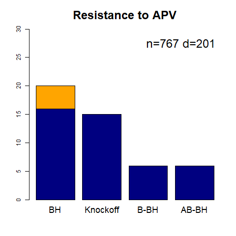
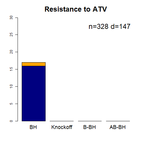
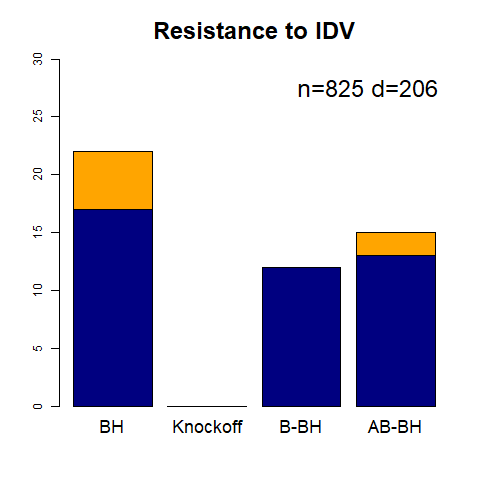
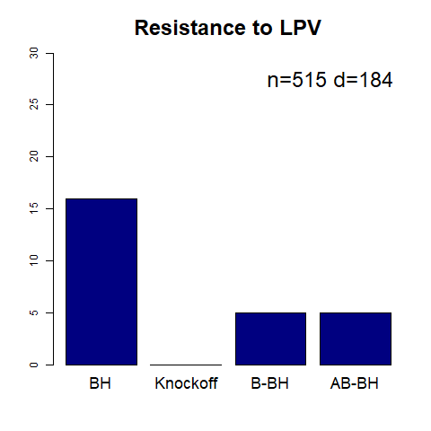
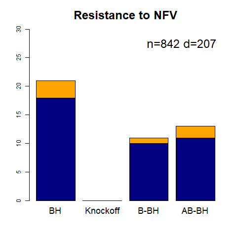
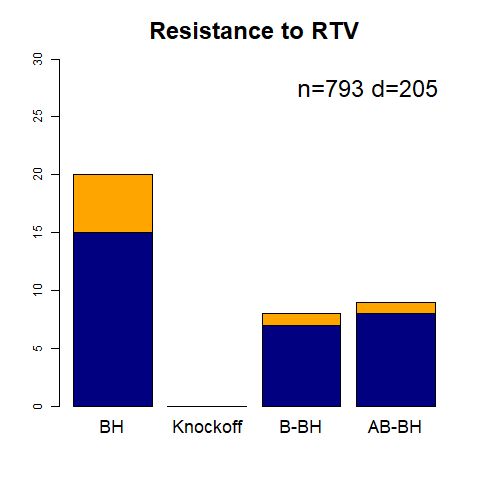
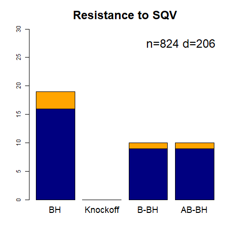
Figure 3: Real data example for $\alpha=0.05$. Blue represents the number of discovers that are in the TSM list; and yellow represents the number of discoveries that not in the TSM list. The total number of HIV-1 protease positions in the TSM list is 34.
BH – the BH method; Knockoff – the knockoff based method of Barber & Candès (2015); B-BH – the proposed Bonferroni-BH method; AB-BH – the proposed adaptive Bonferroni-BH method.

5 Concluding Remarks

This article contributes to the development of new line of research cross-fertilizing two seminal ideas on multiple inference used in modern statistical investigations - use of $p$-value based multiple testing method to control false discoveries (Benjamini & Hochberg, 1995) and use of knockoff copy of the design matrix for variable selection in linear regression settings (Barber & Candès, 2015). Specifically, we introduce novel knockoff-assisted, $p$-value based FDR controlling methods for variable selection in the setting of fixed-design multiple linear regression when sample size is as large as the number of explanatory variables. Underpinning the novelty of our methods is a new understanding of the knockoff’s role in setting the stage for the underlying multiple testing problem. The technical novelty comes from developing new multiple testing methods under this setting with proven control of the FDR under Gaussian noise fully capturing the correlation information on explanatory variables. Our main idea of using knockoffs or generating additional variables to create new settings to successfully control the FDR can have applications outside the scope of this paper. For instance, we can develop FDR controlling methods for multiple testing of Gaussian means with arbitrary but known covariance matrix differently from Fithan & Lei (2020) and Fan et al. (2012). Also, for this same testing problem, we can consider developing methods controlling other overall measures of type I errors, such as FWER (familywise error rate), or $k$-FWER (generalized FWER), or $k$-FDR (generalized FDR). See Lehmann & Romano (2005a) and Sarkar (2008a) for $k$-FWER and Janson & Su (2016)) for the use of $k$-FWER in the context of knockoff assisted variable selection, and Sarkar (2007) for $k$-FDR.

Our proposed methods will continue to work when $X$ is random, irrespective of its distribution, if the conditional distribution of $Y$ given $X$ can be modeled as in (1.1).

On adapting our methods to high-dimensional settings, there are several possibilities. One promising approach would be to develop a two-stage procedure following the line of work in Meinshausen et al. (2009) on controlling the FDR using $p$-values in high-dimensional variable selection based on data-splitting. More specifically, we can consider splitting the data into two parts of equal size. On one part, we can perform variable selection and dimension reduction using one of the existing methods. Meinshausen et al. (2009) gave a list of such methods including the Lasso, the adaptive Lasso, orthogonal matching pursuit, and sure independence screening, which ensure that all important explanatory variables are retained in the selection process under some regularity conditions. Some unimportant variables are allowed to be selected as long as the number of selected variables is less than $n/4$, so that knockoff copies can be created only for the selected variables using the other half of the data. Thus, our proposed knockoff-adjusted BH methods can be applied in the second stage for final selection of important variables. The symmetry of the two parts of the data allows us to implement this two-stage procedure twice, opening up the possibility of developing newer methods combining both results. We would like to pursue this line of research, along with investigating the data-splitting strategy in handling high-dimensional models, in our future work.

6 Acknowledgements

We are grateful to two anonymous referees and the Editor whose valuable suggestions and comments have greatly improved the presentation of our manuscript. We are also thankful to Edo Airoldi and William Fithian for their comments on an earlier version of this paper.

References

- Barber & Candès (2015) Barber, R. F. & Candès, E. J. (2015). Controlling the false discovery rate via knockoffs. Annals of Statistics 43, 2055–2085.
- Barber & Candès (2019) Barber, R. F. & Candès, E. J. (2019). A knockoff filter for high-dimensional selective inference. Annals of Statistics 47, 2504–2537.
- Barber et al. (2020) Barber, R. F., Candès, E. J., & Samworth, R. J. (2020) Robust inference with knockoffs. Annals of Statistics 48, 1409–1431.
- Benjamini & Hochberg (1995) Benjamini, Y. & Hochberg, Y. (1995). Controlling the false discovery rate: a practical and powerful approach to multiple testing. Journal of the Royal Statistical Society: Series B (Methodological) 57, 289–300.
- Benjamini & Yekutieli (2001) Benjamini, Y. & Yekutieli, D. (2001). The control of the false discovery rate in multiple testing under dependency. Annals of Statistics 29, 1165–1188.
- Blanchard & Roquain (2008) Blanchard, G. & Roquain, E. (2008). Two simple sufficient conditions for FDR control. Electronic Journal of Statistics 2, 963–992.
- Blanchard & Roquain (2008) Blanchard, G. & Roquain, E. (2009). Adaptive false discovery rate control under independence and dependence. Journal of Machine Learning Research 10, 2837–2871.
- Candès et al. (2018) Candès, E., Fan, Y., Janson, L. & Lv, J. (2018). Panning for gold: ‘model-x’ knockoffs for high dimensional controlled variable selection. Journal of the Royal Statistical Society: Series B (Statistical Methodology) 80, 551–577.
- Desboulets (2018) Desboulets, L. D. D. (2018) A review on variable selection in regression analysis. Econometrics 6, 1–27.
- Fan et al. (2012) Fan, J., Han, X. & Gu, W. (2012). Estimating false discovery proportion under arbitrary covariance dependence. Journal of the American Statistical Association 107,1019–1035.
- Finner et al. (2007) Finner, H., Dickhaus, T. & Roters, M (2007). Dependency and false discovery rate: Asymptotics. Annals of Statistics 35,1432-–1455.
- Fithan & Lei (2020) Fithian, W. & Lei, L. (2020). Conditional calibration for false discovery rate control under dependence. Manuscript – arXiv:2007.10438v1.
- Janson & Su (2016) Janson, L. & Su, W. (2016). Familywise error rate control via knockoffs. Electronic Journal of Statistics 10, 960–975.
- Karlin (1968) Karlin, S. (1968). Total Positivity. Stanford University Press.
- Karlin & Rinott (1980) Karlin, S. & Rinott, Y. (1980). Classes of ordering of measures and related correlation inequalities: Multivariate totally positive distributions. Journal of Multivariate Analysis 10, 467–498.
- Lehmann & Romano (2005a) Lehmann, E. L. & Romano, J. P. (2005a). Generalizations of the familywise error rate. Annals of Statistics 33, 1138–1154.
- Lehmann & Romano (2005b) Lehmann, E. L. & Romano, J. P. (2005b). Testing Statistical Hypotheses, 3rd Edition. Springer.
- Meinshausen et al. (2009) Meinshausen, P., Meier, L. & Bühlman, P. (2009). p-values for high-dimensional regression. Journal of the American Statistical Association 104,1671–1681.
- Rhee et al. (2005) Rhee, S.-Y., Fessel, W. J., Zolopa, A. R., Hurley, L., Liu, T., Taylor, J., Nguyen, D. P., Slome, S., Klein, D., Horberg, M., Flamm, J., Follansbee, S., Schapiro, J. M. & Shafer, R. W. (2005). HIV-1 protease and reverse-transcriptase mutations: Correlations with antiretroviral therapy in subtype b isolates and implications for drug-resistance surveillance. The Journal of Infectious Diseases 192, 456–465.
- Spector & Janson (2021) Spector, A. & Janson, L. (2021). Powerful knockoffs via minimizing reconstructability. Annals of Statistics, to appear.
- Rhee et al. (2006) Rhee, S.-Y., Taylor, J., Wadhera, G., Ben-Hur, A., Brutlag, D. L. & Shafer, R. W. (2006). Genotypic predictors of human immunodeficiency virus type 1 drug resistance. Proceedings of the National Academy of Sciences 103, 17355–17360.
- Romano et al. (2019) Romano, Y., Sesia, M., & Candès, E. (2019) Deep knockoffs. Journal of the American Statistical Association 115, 1861–1872.
- Sarkar (2002) Sarkar, S. K. (2002). Some results on false discovery rate in stepwise multiple testing procedures. Annals of Statistics 30, 239–257.
- Sarkar (2007) Sarkar, S. K. (2007). Stepup procedures controlling generalized FWER and generalized FDR. Annals of Statistics 35, 2405–2420.
- Sarkar (2008a) Sarkar, S. K. (2008a). Generalizing Simes’ test and Hochberg’s stepup procedure. Annals of Statistics 36, 337–363.
- Sarkar (2008b) Sarkar, S. K. (2008b). On methods controlling the false discovery rate. Sankhyã: The Indian Journal of Statistics 70, 135–168.
- Sesia et al. (2018) Sesia, M., Sabatti, C. & Candès, E. J. (2018). Gene hunting with hidden Markov model knockoffs. Biometrika, 106, 1–18.
- Storey et al. (2004) Storey, J. D., Taylor, J. E. & Siegmund, D. (2004). Strong control, conservative point estimation and simultaneous conservative consistency of false discovery rates: a unified approach. Journal of the Royal Statistical Society: Series B (Statistical Methodology) 66, 187–205.
- Wasserman & Roeder (2009) Wasserman, L. & Roeder, K. (2009). High dimensional variable selection. Annals of Statistics 37, 2178–2201.
- Xing et al. (2019) Xing, X., Zhao, Z. & Liu, J. S. (2019). Controlling false discovery rate using Gaussian mirrors. Manuscript – arXiv:1911.09761.