Critical point determination from probability distribution functions in the three dimensional Ising model

Abstract

In this work we propose a new numerical method to evaluate the critical point, the susceptibility critical exponent and the correlation length critical exponent of the three dimensional Ising model without external field using an algorithm that evaluates directly the derivative of the logarithm of the probability distribution function with respect to the magnetisation. Using standard finite-size scaling theory we found that correction-to-scaling effects are not present within this approach. Our results are in good agreement with previous reported values for the three dimensional Ising model.

I Introduction

The Ising model has a great importance in statistical mechanics since a great variety of techniques and methods, analytical and numerical, have been formulated first on this model. There are several numerical algorithms that can be used to study the critical behavior in spin systems, we can mention three types:

• Those that require adjusting a control parameter, like the standard Monte Carlo or the Wolff algorithms Wolff (1989).

• Algorithms that not required to fine tune any parameter, examples of those kind are the Invasion Cluster Algorithm Machta et al. (1995), algorithms based on Self Organisation Ful (1999) or the Locally Cluster Algorithm Faraggi and Robb (2008).

• Algorithms that evaluate the Density of States in the microcanonical ensemble Wang and Landau (2001); Hüller and Pleimling (2002).

In this work we propose a new methodology based on the algorithm proposed by Sastre et al. for the evaluation of effective temperatures in out of equilibrium Ising-like systems Sastre et al. (2003). The algorithm is a canonical generalisation of the work proposed by Hüller and Pleimling Hüller and Pleimling (2002) for the evaluation of the density of states in the two and three dimensional Ising model. It is important to point out that variations of this algorithm have been successfully implemented in fluids with discrete potential interaction. The microcanonical version was used in Sastre et al. (2015) to evaluate thermodynamic properties in the supercritical region and in Sastre et al. (2018) for the evaluation of the Hight Temperature Expansion coefficients of the Helmholtz free energy. The canonical version Sastre (2020) was used for the evaluation of the critical temperature and the correlation length critical exponent in the Square-Well fluid with interaction range of $1.5$ times the particle diameter.

Our aim in this work is to prove that a completely new methodology can be used to study critical phenomena on Ising-like systems. In particular we want to evaluate the critical temperature and the critical exponents for the correlation length, $\nu$, and the susceptibility, $\gamma$, in the three dimensional Ising model in an efficient way.

This article is organized as follows: in section II we explain the basic definitions for the Ising model and the algorithm used in this work, in section III we apply the method to evaluate the critical point and the critical exponents. We made our concluding remarks in the section IV.

II Probability distributions for the Ising model

For a better understanding of the algorithm used in this work we will review first how the algorithm proposed by Hüller and Pleimling in the microcanonical ensemble works. The algorithm uses a variation of the transition variable method Oli (1998a, b); Kastner et al. (2000) in order to evaluate the entropy as function of the energy and the magnetisation.

The hamiltonian for the Ising model on a three dimensional cubic lattice without external field and nearest neighbors interaction is

$$\frac{1}{k_{B}T}H=-\beta^{-1}\sum_{\langle i,j\rangle}\sigma_{i}\sigma_{j},$$ (1)

where $\sigma_{i}=\pm 1$ is the spin in the $i$ th site, $\beta=k_{B}T/J$ is the control parameter and $J>0$ is the coupling between first nearest neighbor spins. The notation $\langle i,j\rangle$ indicates that the summation runs over all nearest neighbors pairs on the lattice. If we consider a system with periodic boundary conditions and $N=L^{3}$ spins, the magnetisation, $M=\sum_{i}\sigma_{i}$, and the energy will be bounded. Moreover, when a spin is flipped in the system we observe that $\Delta M=\pm 2$ and $\Delta E/J=\pm 4\eta$, $\eta=0,~{}\pm 1,~{}\pm 2,~{}\pm 3$.

In the standard microcanonical notation $\Omega(E_{\mu},M_{k})$ is the number of microstates that share the same magnetisation $M_{k}$ and energy $E_{\mu}$, for simplicity we will use $\Omega_{\mu,k}$ for this number. When the systems is in a given macrostate $\Omega_{\mu,k}$ and we flip a spin at random we can reach a new macrostate $\Omega_{\nu,l}$, with $E_{\nu}=E_{\mu}+4\eta J$ and $M_{k}=M_{l}\pm 2$. The probability of reach $\Omega_{\nu,l}$ starting from $\Omega_{\mu,k}$ will be given by

$$P^{(m)}_{(\mu,k),(\nu,l)}=\frac{V_{(\mu,k),(\nu,l)}}{N\Omega_{\mu,k}},$$ (2)

the superscript $(m)$ denotes that we are working in the microcanonical ensemble and $V_{(\mu,k),(\nu,l)}$ indicates how many ways the system can reach $\Omega_{\nu,l}$ starting from $\Omega_{\mu,k}$, this quantity is purely geometric. We can also obtain the reverse probability with

$$P^{(m)}_{(\nu,l),(\mu,k)}=\frac{V_{(\nu,l),(\mu,k)}}{N\Omega_{\nu,l}}.$$ (3)

As any spin flip can be reversed, the relation $V_{(\mu,k),(\nu,l)}=V_{(\nu,l),(\mu,k)}$ must be satisfied. For example, from the base state with $E_{\mu}=-3NJ$ and $M_{k}=N$ we can reach the state with $E_{\nu}=-3J(N-4)$ and $M_{l}=N-2$ in $N$ ways, then $V_{(\mu,k),(\nu,l)}=N$ and, as $\Omega_{\mu,k}=1$, $P^{(m)}_{(\mu,k),(\nu,l)}=1$. In the reverse process we have $\Omega_{\nu,l}=N$ then $P^{(m)}_{(\nu,l),(\mu,k)}=1/N$. Combining equations (2) and (3) we obtain the important microcanonical relation

$$\frac{P^{(m)}_{(\mu,k),(\nu,l)}}{P^{(m)}_{(\nu,l),(\mu,k)}}=\frac{\Omega_{\nu,l}}{\Omega_{\mu,k}}.$$ (4)

The last equation can be used to evaluate the microcanonical derivatives

$$\frac{1}{T}=\frac{\partial S}{\partial E},$$ (5)

and

$$-\frac{B}{T}=\frac{\partial S}{\partial M},$$ (6)

where $B$ is the magnetic external field. The change on the entropy can be obtained using the following approximation

$$\Delta S=k_{B}\ln\left(\frac{P^{(m)}_{(\mu,k),(\nu,l)}}{P^{(m)}_{(\nu,l),(\mu,k)}}\right)\approx\Delta E\frac{1}{T}-\Delta M\frac{B}{T}.$$ (7)

In the simulation the probabilities can be estimated with the rate of attempts $T_{(\mu,k),(\nu,l)}$ to go from $\Omega_{\mu,k}$ to $\Omega_{\nu,l}$. The rate is given by the relation

$$T_{(\mu,k),(\nu,l)}=\frac{z_{(\mu,k),(\nu,l)}}{z_{(\mu,k)}},$$ (8)

where $z_{(\mu,k)}$ is the number of times that the system spends in a macrostate $\Omega_{\mu,k}$, and $z_{(\mu,k),(\nu,l)}$ is the number of times that the system attempts to change from $\Omega_{\mu,k}$ to $\Omega_{\nu,l}$. In this method, once that we fix the ranges $[E_{min},E_{max}]$ and $[M_{min},M_{max}]$, where the simulation will be confined, the quantities $z_{(\mu,k),(\nu,l)}$ and $z_{(\mu,k)}$ can be estimated in the following way:

1. With $E_{min}\leq E_{\mu}\leq E_{max}$ and $M_{min}\leq M_{k}\leq M_{max}$ as initial state, a spin is chosen at random and $z_{(\mu,k)}$ is always incremented by 1.

2. We evaluate the new values $E_{\nu}$ and $M_{l}$ that the system would take if the chosen spin is flipped.

3. If $E_{min}\leq E_{\nu}\leq E_{max}$ and $M_{min}\leq M_{l}\leq M_{max}$ the quantity $z_{(\mu,k),(\nu,l)}$ is incremented by 1.

4. The spin flip attempt is accepted with probability $\min{(1,\frac{z_{(\nu,l),(\mu,k)}z_{(\mu,k)}}{z_{(\mu,k),(\nu,l)}z_{(\nu,l)}})}$. This condition assures that all macrostates are visited with equal probability, independently of their degeneracy.

The values $z_{(\mu,k),(\nu,l)}$ and $z_{(\mu,k)}$ can be initialized with any positive integer, a safe option is $1$, and after a large number of spin flip attempts we will observe that $T_{(\mu,k),(\nu,l)}\to P_{(\mu,k),(\nu,l)}$.

Müller an Pleimling used this method for the determination of the microcanonically defined spontaneous magnetisation and the order parameter critical exponent for the Ising model in two and three dimensions. This algorithm is highly efficient for evaluate the ratios $\Omega_{\nu,l}/\Omega_{\mu,k}$ since it gives the freedom of restricting the calculations to a chosen range in the energy and magnetisation. Additional details of the method can be found in the original work Hüller and Pleimling (2002).

The microcanonical algorithm counts all the attempts to change from a given macrostate to another, as long as the final macrostate is an allowed one, while the generalisation proposed in Sastre et al. (2003) adds an additional condition to the attempts count. The additional condition includes a ”heat bath”, then we will need to incorporate an extra factor in the ratio of probabilities

$$\frac{P_{(\mu,k),(\nu,l)}}{P_{(\nu,l),(\mu,k)}}=\frac{P^{(m)}_{(\mu,k),(\nu,l)}}{P^{(m)}_{(\nu,l),(\mu,k)}}e^{-\frac{\Delta E}{k_{B}T}}=\frac{\Omega_{\nu,l}}{\Omega_{\mu,k}},e^{-\frac{\Delta E}{k_{B}T}}$$ (9)

here the absence of the superscript indicates that we are no longer in the microcanonical ensemble. Combining Equations (7) and (9) we get

$$\ln({P_{(\mu,k),(\nu,l)}})-\ln({P_{(\nu,l),(\mu,k)}})\approx-\Delta M\frac{B}{k_{B}T},$$ (10)

where we can drop the subscript $\mu$ and $\nu$, since the right hand side of the equation depends only on $\Delta M$. In the simulation the probabilities now can be estimated with the rate of attempts $T_{kl}$ to go from a macrostate with magnetisation $M_{k}$ (level $k$) to a macrostate with magnetisation $M_{l}$ (level $l$). The quantity $T_{kl}$ will be given now by the relation

$$T_{kl}=\frac{z_{kl}}{z_{k}},$$ (11)

where $z_{kl}$ is the number of times that the system attempts to change from level $k$ to level $l$ and $z_{k}$ is the number of times that the system spends in level $k$. For the estimation of the $z_{kl}$ and $z_{k}$ values, the detailed steps are now:

1. With $M_{min}\leq M_{k}\leq M_{max}$ as initial state, a spin is chosen at random and $z_{k}$ is always incremented by 1.

2. If the possible state $M_{l}$, that would be reached if the chosen spin is flipped, is allowed we evaluate $\Delta E$ between states $M_{k}$ and $M_{l}$, and the quantity $z_{kl}$ is incremented by 1 with probability $\min(1,e^{-\Delta E/k_{B}T})$.

3. The spin flip attempt is accepted with probability $\min{(1,\frac{z_{lk}z_{k}}{z_{kl}z_{l}})}$.

The values $z_{kl}$ and $z_{k}$ are initialized to 1 and after a large number of spin flip attempts we will observe that $T_{kl}\to P_{kl}$.

Now we obtain the derivative of $\ln{P}$, instead of the derivatives of $S$, with the following approach

$$\left.\frac{\partial\ln{P}}{\partial M}\right|_{k}\approx\ln{P_{kl}}-\ln{P_{lk}}\approx\ln(T_{kl}/T_{lk}).$$ (12)

We will use the following function in our simulations

$$g(m)=L^{-d}\frac{\partial\ln P}{\partial m},$$ (13)

where $m=M/L^{d}$, since it can be obtained directly from the transition rates with the approximation

$$g(m_{k})\approx\frac{1}{2}\left(\ln[(T_{k,k+1})/(T_{k+1,k})]-\ln[(T_{k,k-1})/(T_{k-1,k})]\right),$$ (14)

where $T_{k,k\pm k}$ are the transition rates from level $k$ to its adjacent levels and $T_{k\pm 1,k}$ are the transition rates from the adjacent levels to level $k$.

We verified that this method is compatible with the ansatz proposed by Tsypin and BlöteTsypin and Blöte (2000) for the three dimensional Ising model at the critical point

$$P(m)\sim\exp{\left[-\left(\left(\frac{m}{m_{0}}\right)^{2}-1\right)^{2}\left(a\left(\frac{m}{m_{0}}\right)^{2}+c\right)\right]},$$ (15)

where $a,~{}c$ and $m_{0}$ are size depending fitting parameters. For $L=12$ we performed three independent simulations at $\beta_{c}=0.221654$, taken from Ref. Campbell and Lundow (2011), with different ranges in $m$. Our results are show in Figure 1 along with the curve given by Eq. (15), using $a=0.268$, $c=0.268$, $m=0.3892$. Our simulations are in really good agreement with the ansatz, except at the extreme values of the curves, but this effect is also present in the results published by Tsypin and Blöthe.

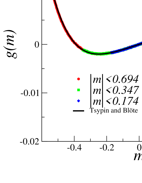
Figure 1: (Color online) Graph of $g$ as function of $m$ for three different range simulations. We observe that the restriction in range does not affects the computed value of $g$. The continuous line reproduces Eq. (15) with the parameters $a=0.268,~{}c=0.859$ and $m_{0}=0.3892$ for $L=12$. There is a really good agreement with our results, except in the extremes of the curves, as shown in the inset.

III Results

Now we will explain how to obtain the critical temperature and the correlation length critical exponent. It is a well known fact that there is a change in the probability distribution of the order parameter above and below a certain value of $\beta$, denoted as $\beta_{c}(L)$, that depends on the system size. For $\beta$ values below $\beta_{c}(L)$ there is just one peek at $m=0$, that means that the curve $g(m)$ crosses the horizontal axis with a negative slope. For $\beta$ values above $\beta_{c}(L)$ there are two peeks at $m=\pm m_{sta}$ in the probability distribution, while $g(m)$ crosses the horizontal axis in three places, at $m=\pm m_{sta}$ with a negative slope and at $m=0$ with a positive slope. In Figure 2 we can see clearly the symmetry breaking for three dimensional Ising model with linear size $L=8$.

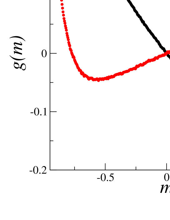
Figure 2: (Color online) Symmetry breaking for the three dimensional Ising model with $L=8$. For $\beta<\beta_{c}$ the curve cross the horizontal axis at $m=0$ with a negative slope. For $\beta>\beta_{c}$ we have three crossings, at $m=0$ and at $m=\pm m_{sta}$ and we observe that the slope at $m=0$ is now positive.

As we can see there is a change in the sign of the slope $\partial g/\partial m$ around $m=0$ as function of $\beta$, then we can find $\beta_{c}(L)$ restricting our simulations around $m=0$. We performed simulations restricting the intervals to $|m|\lesssim 0.1$ on several system sizes and temperature values in the three dimensional Ising model. The justification for this interval is that $g(m)$ is linear around $m=0$ and the slope can be easily obtained from a linear fit to the simulation data. For every system size we evaluate the slope for several values of $\beta$, in Figure 3 we are illustrating how the evaluation of $\beta_{c}(L)$ is performed for the case $L=12$. Here we used a linear fit to the curves of the slope as function of $\beta$ in order to solve $\left(\frac{\partial g}{\partial m}\right)_{\beta=\beta_{c}}=0$.

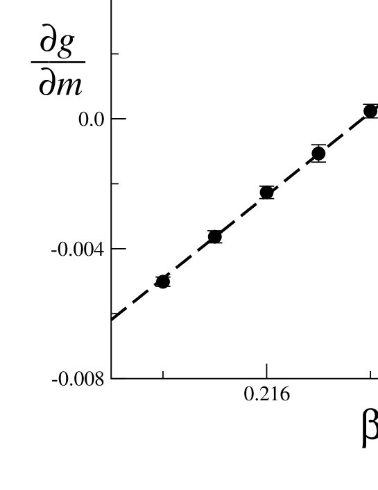
Figure 3: Slopes of the function $g(m)$ at $m=0$ for the three dimensional Ising model with $L=12$ as function of the control parameter $\beta$. The dashed line is a linear fit to the simulation data.

From here we can use the Finite size scaling ansatz for the critical temperature, given by the relation

$$\beta_{c}(L)\approx\beta_{c}+AL^{-1/\nu},$$ (16)

where $\beta_{c}$ is the critical control parameter for the infinite system, $A$ is a non universal parameter and $\nu$ is the critical exponent for the correlation length Ferrenberg and Landau (1991). In principle Eq. (16) is valid for sufficiently large $L$ values. For small systems the last term changes to $L^{-1/\nu}(1+BL^{-\omega})$, here the parameter $\omega$ is the scale correction exponent, whose reported value for the three dimensional Ising model is $\omega\approx 0.81$ Lundow and Campbell (2010).

The simulations were carried out in systems with linear sizes $L=8$, 10, 12, 14, 16, 20 and 24, using $5N\times 10^{6}$ spin flip attempts and 120 independent runs for every set of parameters. With these values we obtain reliable data with less CPU time compared with standard canonical simulations, since most of the spin flips are discarded when the system falls outside of the restricted range. However, all attempts, successful or not, are used for the evaluation of the transition rates. We evaluated $T_{c}$ and $\nu$ performing a non-linear curve fitting to Eq. (16), in Figure 4 we show the evaluation of the critical point along with the $\nu$ critical exponent. We must emphasized that in our analysis the scale correction exponent is absent, which is a great advantage in numerical simulations that study critical phenomena. This feature is also observed in the evaluation of the critical temperature for the square-well fluid using an equivalent method Sastre (2020). We think that the absence of scale corrections are related to the fact that in this method we evaluate the critical point analyzing the behavior of the probability distribution of the order parameter around $M=0$, while in most traditional methods the critical point is evaluated analyzing the behavior around the peaks of the probability distribution.

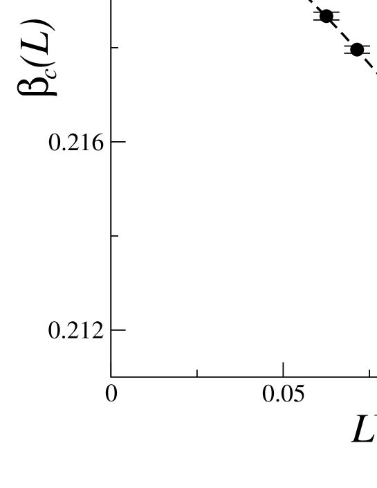
Figure 4: Evaluation of the critical temperature and the correlation length critical exponent for the three dimensional Ising model. The dashed line is a non-linear curve fit to Eq. (16). The results from the fit are $\beta_{c}=0.22165$, $A=-0.2439$ and $1/\nu=1.587$.

The results for the critical point is $\beta_{c}=0.22165(65)$ and for the correlation length critical exponent we obtain $\nu=0.6301(88)$, that are in good agreement with previous reported values, see Table 1.

Table 1: Critical parameters for the three dimensional Ising model obtained in this work and those from literature. The values between parenthesis indicate the uncertainty in the lasts digits.

$\beta_{c}$	$\nu$	Source
0.22165(65)	0.6301(88)	This work
0.22165452(8)	0.63020(12)	Butera and Comi Butera and Comi (2002)
0.221655(2)	0.6299(2)	Deng and Blöte Deng and Blöte (2003)
0.221654(2)	0.6308(4)	Lundow and Campbell Lundow and Campbell (2010)

Once that we have the critical temperature we can proceed to evaluate the susceptibility critical exponent $\gamma$. We used the scaling ansatz for the probability distribution function at the critical point proposed in Ref. Kaski et al. (1984)

$$P(m,L)\approx\exp{(-A_{0}+A_{2}x^{2}+A_{4}x^{4}+\dots)},$$ (17)

where $x=mL^{\beta/\nu}<<1$ and $\beta$ is the order parameter critical exponent. As we are restricting our simulations to the range $|m|\leq 0.1$ we can use the next approximation

$$\frac{\partial\ln{P}}{\partial m}=2A_{2}mL^{2\beta/\nu}+O(x^{3}),$$ (18)

that we can combine with Eq. (13) to obtain the desired scaling relation

$$\frac{\partial g}{\partial m}\sim L^{-\gamma/\nu}.$$ (19)

For the three dimensional case we performed simulations at our estimated critical point $\beta_{c}=0.22165$ and linear sizes $L=8$, 10, 12, 14, 16, 20 and 24. In this case we used $N\times 10^{7}$ spin flip attempts and 120 independent runs for every $L$ value. The critical exponent $\gamma$ was obtained from a linear fit to Eq. (19) as shown in Figure 5. From this fit we obtain $\gamma/\nu=1.973(10)$ that is also in good agreement with the reported value $\gamma/\nu=1.9632(6)$ Campbell and Lundow (2011). Again we observe that scaling correction exponents are absent.

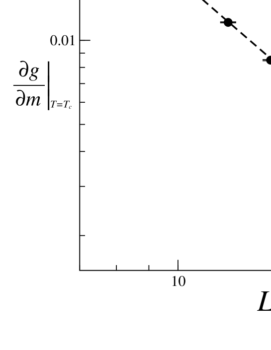
Figure 5: Evaluation of the critical exponent $\gamma/\nu$ for three dimensional Ising model. We are showing a log-log graph of the derivatives $\partial g/\partial m$ as function of the linear size $L$. The dashed line is the linear fit to Equation (19). From the fit we obtain the slope $\gamma/\nu=1.973$.

IV Conclusions

We have presented a new method for the evaluation of the critical temperature and the critical exponents for the correlation length $\nu$ and the susceptibility $\gamma$ on the three dimensional Ising model. Using the derivatives of the probability distribution function for the magnetisation and small system sizes we obtain reliable results that are in good agreement with the reported values. The method can be used in a restricted range on the magnetisation and this feature reduces the computational time in the simulations. One additional advantage of the method is that scale corrections are not present, at least in the three dimensional Ising model. In future works we will study if this advantage is present in other systems.

V Acknowledgements

This research was supported by Universidad de Guanajuato (México) under Proyecto DAIP 879/2016 and CONACyT (México)(grant CB-2017-2018-A1-S-30736-F-2164).

References

References

- Wolff (1989) U. Wolff, Phys. Rev. Lett. 62, 361 (1989).
- Machta et al. (1995) J. Machta, Y. S. Choi, A. Lucke, T. Schweizer, and L. V. Chayes, Phys. Rev. Lett. 75, 2792 (1995).
- Ful (1999) Physica A: Statistical Mechanics and its Applications 264, 171 (1999), ISSN 0378-4371.
- Faraggi and Robb (2008) E. Faraggi and D. T. Robb, Phys. Rev. B 78, 134416 (2008).
- Wang and Landau (2001) F. Wang and D. P. Landau, Phys. Rev. Lett. 86, 2050 (2001).
- Hüller and Pleimling (2002) A. Hüller and M. Pleimling, International Journal of Modern Physics C 13, 947 (2002).
- Sastre et al. (2003) F. Sastre, I. Dornic, and H. Chaté, Phys. Rev. Lett. 91, 267205 (2003).
- Sastre et al. (2015) F. Sastre, A. L. Benavides, J. Torres-Arenas, and A. Gil-Villegas, Phys. Rev. E 92, 033303 (2015).
- Sastre et al. (2018) F. Sastre, E. Moreno-Hilario, M. G. Sotelo-Serna, and A. Gil-Villegas, Molecular Physics 116, 351 (2018).
- Sastre (2020) F. Sastre, Molecular Physics 118, e1593534 (2020).
- Oli (1998a) The European Physical Journal B - Condensed Matter and Complex Systems 1 (1998a), ISSN 1434-6028.
- Oli (1998b) The European Physical Journal B - Condensed Matter and Complex Systems 6 (1998b), ISSN 1434-6028.
- Kastner et al. (2000) M. Kastner, M. Promberger, and J. D. Muñoz, Phys. Rev. E 62, 7422 (2000).
- Tsypin and Blöte (2000) M. M. Tsypin and H. W. J. Blöte, Phys. Rev. E 62, 73 (2000).
- Campbell and Lundow (2011) I. A. Campbell and P. H. Lundow, Phys. Rev. B 83, 014411 (2011).
- Ferrenberg and Landau (1991) A. M. Ferrenberg and D. P. Landau, Phys. Rev. B 44, 5081 (1991).
- Lundow and Campbell (2010) P. H. Lundow and I. A. Campbell, Phys. Rev. B 82, 024414 (2010).
- Butera and Comi (2002) P. Butera and M. Comi, Phys. Rev. B 65, 144431 (2002).
- Deng and Blöte (2003) Y. Deng and H. W. J. Blöte, Phys. Rev. E 68, 036125 (2003).
- Kaski et al. (1984) K. Kaski, K. Binder, and J. D. Gunton, Phys. Rev. B 29, 3996 (1984).