Sample-path large deviations for stochastic evolutions driven by the square of a Gaussian process.

Abstract

Recently, a number of physical models has emerged described by a random process with increments given by a quadratic form of a fast Gaussian process. We find that the rate function which describes sample-path large deviations for such a process can be computed from the large domain size asymptotic of a certain Fredholm determinant. The latter can be evaluated analytically using a theorem of Widom which generalizes the celebrated Szegő-Kac formula to the multi-dimensional case. This provides a large class of random dynamical systems with time scale separation for which an explicit sample-path large deviation functional can be found. Inspired by problems in hydrodynamics and atmosphere dynamics, we construct a simple example with a single slow degree of freedom driven by the square of a fast multi-variate Gaussian process and analyse its large deviations functional using our general results. Even though the noiseless limit of this example has a single fixed point, the corresponding large deviations effective potential has multiple fixed points. In other words, it is the addition of noise that leads to metastability. We use the explicit answers for the rate function to construct instanton trajectories connecting the metastable states.

I Introduction

Large deviation theory recently became a key theoretical tool for the statistical mechanics of non equilibrium systems. Describing sample-path large deviations for the dynamics of effective degrees of freedom leads to a precise understanding of typical and rare trajectories of physical, biological or economic processes. A paradigm example for the effective descriptions of complex systems using large deviation theory is the macroscopic fluctuation theory of systems of interacting particles [1]. However, for genuine non-equilibrium processes, without local detailed balance, the class of systems for which the rate function can be found explicitly is extremely limited.

In this paper, we consider a class of systems for which the effective dynamics has increments which are given by a quadratic form of a fast Gaussian process. This type of stochastic driving is relevant for many applications. Quadratic interactions are common in many physical examples such as hydrodynamics, plasmas described by the Vlasov equation, magneto hydrodynamics, self gravitating systems, the KPZ equation, quadratic networks (for instance heat transfer across quadratic networks [2]), to cite just a few. For all these systems with quadratic nonlinearities, in some regime a separation of time scale exists and the effective degrees of freedom are coupled to fast evolving Gaussian processes. This is the case, for example, for the kinetic theories of plasma [3, 4], self gravitating systems [5], geostrophic turbulence [6], wave turbulence [7] for some specific dispersion relations, among many other examples. From a theoretical and mathematical perspective, modelling the driver of the effective degrees of freedom by a quadratic form of a fast Gaussian process proves to be a decisive simplification. With this assumption, we will be able to write explicit formulae for the sample-path large deviation rate function, and proceed to its analysis in many interesting examples.

The study of a slow process coupled to a fast one is a classical paradigm of physics and mathematics, the celebrated Kapitza pendulum [8] being a canonical example. For such fast/slow dynamics, one can study the averaging of the effect of the fast variable on the slow one (law of large numbers), or the typical fluctuations (stochastic averaging [9]), or the rare fluctuations described by the large deviations theory [10]. The latter is a natural tool for describing the evolution of metastable systems consisting of long periods spent near an equilibrium point interspersed by rare transitions to a distinct equilibrium along an almost deterministic ’instanton’ trajectory. A number of systems with time-scale separation and drift quadratic in fast variables exhibit metastability, see e. g. [11], [12] and references therein.

The large deviation theory has been developed for slow/fast Markov processes  [13, 14] or deterministic systems [15, 16]. Unfortunately, there are not many examples of fast/slow systems for which the large deviations rate function is known explicitly, which would enable the study of detailed properties of the systems such as the equilibrium points and transition trajectories connecting them.

A pedagogical review of the large deviation theory for systems of stochastic differential equations (SDE’s) with two well separated time scales can be found in [17]. The theory is illustrated by a class of examples such that the drift for the slow process is given by a second degree polynomial of the fast process. The corresponding large deviations principle is expressed in terms of the solution of a matrix Ricatti equation. Unfortunately, the resulting expression is not explicit enough to study the practically important phenomenon of stochastically generated metastability: all metastable models considered in [17] already possess multiple fixed points in the noiseless limit. The turbulent models discussed in [18] suffer from the same flaw: metastability appears due to a careful choice of the potential rather than being generated dynamically.

The main new contribution of the current work is two-fold. Firstly, we apply the asymptotic theory of Fredholm determinants to the calculation of the large deviation rate function; this results is an explicit formula for the rate function which characterizes sample-path large deviations for the slow process in terms of a finite-dimensional determinant of a matrix of the size equal to the number of fast degrees of freedom. Essentially, Szegő’s theory of Fredholm determinants is used to build an asymptotic solution to the matrix Ricatti equation of [17].

Secondly, we introduce a concrete illustrative example with stochastically generated metastability. This is a system of stochastic differential equations with a single slow variable and a multi-dimensional fast variable for which all the drifts are quadratic such that in the noiseless limit there is a unique fixed point. However, the addition of noise leads to the appearance of multiple fixed points for the effective Hamiltonian dynamics describing the sample-path deviations. In other words the noisy system exhibits metastability. We use our explicit knowledge of the rate function to construct transition paths (instanton trajectories) between the fixed points.

A third result of our paper is of a more technical nature: as it turns out, it is enough to characterise the fast variables as a Gaussian process with the auto-correlation function which decays sufficiently fast, for example exponentially. In particular, it is not necessary to require that the fast process be Markov. Relaxing this assumption opens up a possibility of using our results in turbulence modelling in the following way: the auto-correlation functions of the small scale turbulence are measured experimentally and used to model the small scale fluctuations as a fast Gaussian process. Then the large deviations properties of the large scale turbulence can be studied theoretically using the theory described below. A rigorous validation of the large deviations principle without assuming Markovianity is also a very natural question for the probability theory.

It is worth stressing that the current paper does not deal with applications of the developed theory to specific physical systems. However, it has been already proved useful for the study of large deviations in a mean field model of plasma kinetics, see the recent preprint [19] for details. We also hope that we can apply the explicit formulas found here to understand the hydrodynamic bistability discussed in  [11, 12].

The rest of the paper is organised as follows. We start with the definition of the model in Section II and give a heuristic derivation of the corresponding large deviation principle in Section III. The highlight of this section is the application of Widom’s theorem for the asymptotics of Fredholm determinants to the calculation of the rate function. In Section IV we show the emergence of metastability for a particular representative of our class of models and study the corresponding ’instanton’ trajectories. Brief conclusions are presented in Section V. Appendices A, B, C contains some technical derivations for Section III. Appendix D contains a review of Widom’s theorem.

II Slow dynamics quadratically driven by a fast Gaussian process

Consider the following stochastic model:

$$\left\{\begin{array}[]{ccl}\dot{X}(t)&=&Y^{T}\left(\frac{t}{\epsilon},X(t)\right)MY\left(\frac{t}{\epsilon},X(t)\right)-\nu X(t),\\ X(0)&=&x_{0},\end{array}\right.$$ (3)

where $\{X(t)\}_{t\geq 0}$ is an $\mathbb{R}^{n}$-valued random process, $\epsilon$ is a parameter, which determines time scale separation between the processes $X$ and $Y$, $0<\epsilon<<1$; for a fixed $x\in\mathbb{R}^{n}$, $(Y(t,x),t,x\in\mathbb{R})$ is an $N$-dimensional time-stationary centred Gaussian process with the auto-correlation function (covariance matrix)

$$C_{ij}(\tau,x,y)=\mathbb{E}\left[Y_{i}(t,x)Y_{j}(t+\tau,y)\right],$$ (4)

$$\text{where }\tau\geq 0,1\leq i,j\leq N,$$

which is assumed to be continuous in all the arguments $\tau,x,y$. As we will see, only $C(\tau,x,x)$ enters the final expression for the large deviation rate function, which justifies our shorthand notation $C(\tau,x):=C(\tau,x,x)$. Finally, $M$ is a $n\times N\times N$ matrix, symmetric with respect to the permutation of the last two indices, and $\nu>0$ is a parameter. Notice that the $(X,Y)$ process need not be Markov.

We assume that $C(\tau,x)$ decays at least exponentially with $\tau$, perhaps uniformly with respect to $x$. Then, in the limit of $\epsilon\rightarrow 0$, the slow random process $X$ stays near the solution to the deterministic equation

$$\left\{\begin{array}[]{ccl}\dot{x}(t)&=&\text{tr}\left[MC(0,x(t))\right]-\nu x(t),\\ x(0)&=&x_{0},\end{array}\right.$$ (7)

where tr is the trace over $N$ ’fast’ indices. Equation (7) is a consequence of the ergodic average applied to the integral form of (3). The typical fluctuations of $X(t)$ around $x(t)$ are Gaussian, with covariance of order $\epsilon$ (more precisely, the distribution of $\lim_{\epsilon\rightarrow 0}$ $\frac{X(t)-x(t)}{\sqrt{\epsilon}}$ is centred Gaussian). Here we are interested in the statistics of large deviations of $X(t)$ when $X(t)-x(t)=O(1)$, which are no longer Gaussian in general.

III Large deviation principle for paths of the slow process

If the fast process were Markov, the starting point for our analysis would be the known large deviations principle for fast-slow Markov systems expressed in terms of the Legendre transform of the cumulant generating functional

$$Z_{T}[x,\lambda]\!\!=\!\!\log\mathbb{E}_{Y}\exp\left\{\!\!\int_{0}^{T}\!\!\!\!dt\lambda(t)f\left(x(t),Y(t,x(t))\right)\right\},$$ (8)

where $f$ is the right hand side of the equation (3) for the slow degrees of freedom, see [17] for a review.

However, it turns out that assuming the Gaussianity of $Y$ and the exponential decay of the corresponding auto-correlation function it is possible to arrive at a counterpart of (8) without assuming Markovianity, see Eq. (9) below. As we already explained in the introduction, by extending the range of possible drivers we open up a possibility of applying our results to turbulent modelling.

The following is essentially a computation of the functional integral measure for the slow variable $X$, which we have to use instead of the Martin-Siggia-Rose method [20], which is only applicable to the Markov case. It is not a proof, but rather a heuristic argument devised to give an intuitive feel for the conjectured form of the large deviation principle. Let us fix the final time $t>0$, choose a large integer $P\in\mathbb{N}$ and a positive number $\eta$ and define

$$\Delta t=\frac{t}{P},~{}b_{\eta}(x)=\prod_{\alpha=1}^{n}[x_{\alpha}-\eta,x_{\alpha}+\eta],$$

where $x$ is a point in $\mathbb{R}^{n}$ and $\prod$ stands for the direct product of intervals. Geometrically, $b_{\eta}(x)$ is a hypercube in $\mathbb{R}^{n}$ centred on $x$ with side $2\eta$. Let $(\lambda_{1},\lambda_{2},\ldots,\lambda_{P})$, $(x_{1},x_{2},\ldots,x_{P})$ be two sequences of $n$-dimensional vectors. Let $\mathbb{P}$ be the probability distribution for the process $(X,Y)$. Let $\mathbb{E}$ be the corresponding expectation. We are interested in the probability that at the times $k\Delta t$ the corresponding values of the slow process $X(k\Delta t)$ are near the points $x_{k}$ , $1\leq k\leq P$. A computation exploiting Chebyshev’s inequality shows that for any sequence of $\lambda$’s

$$\epsilon\log\mathbb{P}\left[X(k\Delta t)\in b_{\eta}(x_{k}),k=1,\ldots,P\right]\leq$$ (9)

$$\sum_{k=1}^{P}\!\!\bigg{(}\!\!\lambda_{k}^{T}\left(x_{k-1}\!-\!x_{k}\right)\!\!+\!\!\epsilon\log\mathbb{E}\left[e^{\lambda_{k}^{T}F(Y,x_{k-1})}\right]\!\bigg{)}\!\!+\!\!R(\epsilon,\Delta t,\eta),$$

where

$$F(Y,x)=\int_{0}^{\Delta t/\epsilon}d\tau Y^{T}(\tau,x)MY(\tau,x)-\nu x\Delta t/\epsilon,$$ (10)

and $R$ is an error term depending on $\epsilon$, $\eta$ and $\Delta t$ such that for $\eta=\mu\Delta t$,

$$\lim_{\mu\rightarrow 0}\lim_{\Delta t\rightarrow 0}\lim_{\epsilon\rightarrow 0}R(\epsilon,\Delta t,\mu\Delta t)=0.$$ (11)

The derivation of (9) is based on the approximation of $Y$ by a bounded process with a finite dependency range. It is carried out in Appendix A. Here we would only like to point out that the dependence on $\lambda$ in the right hand side of (9) appears due to the repeated use of Chebyshev’s inequality. Intuitively, the sequence $(\lambda_{k})$ is the discretised counterpart of the response field appearing in Martin-Siggia-Rose computation.

The next aim is to compute the expectation

$$\mathbb{E}\left[e^{\lambda^{T}F(Y,x)}\right]\!\!=\!e^{-\frac{\Delta t}{\epsilon}\nu\lambda^{T}x}\mathbb{E}\left[e^{\lambda^{T}\left(\int_{0}^{\Delta t/\epsilon}d\tau Y^{T}(\tau,x)MY(\tau,x)\right)}\right],$$

which can be done using the fact that for a fixed $x\in\mathbb{R}^{n}$ the process $Y(\cdot,x)$ is stationary and Gaussian. What follows is the key computation of the paper linking averaging over fast Gaussian fields with the asymptotic of certain Fredholm determinants. Let us define $m:=\lambda^{T}M$, an $N\times N$ symmetric matrix. It can be decomposed as $m=S^{T}S$, where $S$ is a possibly complex Cholesky factor of $m$. Rewrite

$$\exp\left[\lambda^{T}\left(\int_{0}^{\Delta t/\epsilon}d\tau Y^{T}(\tau,x)MY(\tau,x)\right)\right]$$

$$=\int\prod_{\tau}\mathfrak{D}q(\tau)e^{-\frac{1}{4}\int_{0}^{T}d\tau q^{T}(\tau)q(\tau)+\int_{0}^{\Delta t/\epsilon}d\tau q^{T}(\tau)SY(\tau,x)}$$

(Hubbard-Stratonovich transformation). Then, for sufficiently small components of $\lambda$,

$$\mathbb{E}\exp\left[\lambda^{T}\left(\int_{0}^{\Delta t/\epsilon}d\tau Y^{T}(\tau,x)MY(\tau,x)\right)\right]$$

$$=\!\!\int\!\!\prod_{\tau}\!\!\mathfrak{D}q(\tau)e^{-\frac{1}{4}\int_{0}^{\frac{\Delta t}{\epsilon}}\!\!\!\!d\tau q^{T}(\tau)q(\tau)}\mathbb{E}\left(e^{\int_{0}^{\frac{\Delta t}{\epsilon}}\!\!\!\!d\tau q^{T}(\tau)SY(\tau,x)}\right)$$

$$=\!\!\int\prod_{\tau}\mathfrak{D}q(\tau)\exp\bigg{[}-\frac{1}{4}\int_{0}^{\Delta t/\epsilon}d\tau q^{T}(\tau)q(\tau)$$

$$+\frac{1}{2}\int_{0}^{\Delta t/\epsilon}\!\!\!\!d\tau_{1}\int_{0}^{\Delta t/\epsilon}\!\!\!\!d\tau_{2}q^{T}(\tau_{1})SC(\tau_{1}-\tau_{2},x)S^{T}q(\tau_{2})\bigg{]}$$ (12)

$$=\text{Det}^{-\frac{1}{2}}\!\!\left(I\!-\!2S\hat{C}_{\Delta t/\epsilon}(x)S^{T}\right)=\text{Det}^{-\frac{1}{2}}\!\!\left(I\!-\!2m\hat{C}_{\Delta t/\epsilon}(x)\right).$$

Here $m\hat{C}_{\Delta t/\epsilon}(x)$ is an integral operator acting on (square integrable) $\mathbb{R}^{N}$-valued functions on $[0,\Delta/\epsilon]$ as follows:

$$f_{\alpha}(t)\!\!\mapsto\!\!m\hat{C}_{\Delta t/\epsilon}(x)(f)_{\alpha}(t)\!\!$$ (13)

$$= \!\!\sum_{\beta,\delta=1}^{N}\int_{0}^{\Delta t/\epsilon}d\tau m_{\alpha\beta}C_{\beta,\delta}(t-\tau,x)f_{\delta}(\tau),$$

for all $\alpha=1,\ldots,N;t\in[0,\Delta t/\epsilon]$.

In what follows we will use capital Det and Tr to denote operator determinant and trace, and reserve the lowercase $\det$ and tr for the determinant and the trace of finite-dimensional matrices.

The calculation of (12) in the limit $\epsilon\rightarrow 0$ requires the asymptotic analysis of the Fredholm determinant of an integral operator acting on functions defined on a large interval. Fortunately, such an asymptotic can be computed using Widom’s theorem, which generalises the celebrated Szegő-Kac formula for Fredholm determinants, see [21]: for a sufficiently small $m$ (e.g. with respect to a matrix norm),

$$\log\text{Det}\left(I-2m\hat{C}_{\Delta t/\epsilon}(x)\right)$$ (14)

$$= \frac{\Delta t}{\epsilon}\int_{\mathbb{R}}\frac{dk}{2\pi}\log\det\left(I-2m\tilde{C}(k,x)\right)+O\left(1\right),$$

where $\tilde{C}(k,x)=\int_{\mathbb{R}}d\tau e^{ik\tau}C(\tau,x)$ is the Fourier transform of the autocorrelation function $C(\tau,x)$. This remarkable statement is reviewed in Appendix D. Substituting (12), (14) into (9) we find

$$\epsilon \!\!\!\!\log\mathbb{P}\left[X(p\Delta t)\in b_{\eta}(x_{p}),p=1,\ldots,P\right]$$ (15)

$$\stackrel{{\scriptstyle(\ref{step0})}}{{\leq}} \sum_{p=1}^{P}\Delta t\lambda_{p}^{T}\left(\frac{x_{p-1}-x_{p}}{\Delta t}-\nu x_{p-1}\right)+\sum_{p=1}^{P}\epsilon\log\mathbb{E}\exp\left[\int_{0}^{\Delta t/\epsilon}d\tau Y^{T}(\tau,x_{p-1})mY(\tau,x_{p-1})\right]+R$$

$$\stackrel{{\scriptstyle(\ref{fdet1})}}{{=}} \sum_{p=1}^{P}\Delta t\lambda_{p}^{T}\left(\frac{x_{p-1}-x_{p}}{\Delta t}-\nu x_{p-1}\right)-\frac{1}{2}\sum_{p=1}^{P}\epsilon\log\text{Det}\left(I-2m\hat{C}_{\frac{\Delta t}{\epsilon}}(x_{p-1})\right)+R$$

$$\stackrel{{\scriptstyle(\ref{fdet2})}}{{=}} \sum_{p=1}^{P}\Delta t\lambda_{p}^{T}\left(\frac{x_{p-1}-x_{p}}{\Delta t}-\nu x_{p-1}\right)-\frac{1}{2}\sum_{p=1}^{P}\epsilon\left[\frac{\Delta t}{\epsilon}\int_{\mathbb{R}}\frac{dk}{2\pi}\log\det\left(I-2m\tilde{C}(k,x_{p-1})\right)\right]+R+O(\epsilon P)$$

$$= \sum_{p=1}^{P}\Delta t\lambda_{p}^{T}\left(\frac{x_{p-1}-x_{p}}{\Delta t}-\nu x_{p-1}\right)-\frac{1}{2}\sum_{p=1}^{P}\Delta t\int_{\mathbb{R}}\frac{dk}{2\pi}\log\det\left(I-2\lambda_{p}^{T}M\tilde{C}(k,x_{p-1})\right)+R+O(\epsilon P),$$

where the $O(\epsilon P)$ addition to the error term comes from the $O(1)$ term in (14). The expression (15) is an upper bound on the (discretisation of) the functional integral measure for the process $X$.

The next step is akin to the calculation of a path integral for $\epsilon\rightarrow 0$ using the Laplace method. The question we ask is: what is the probability $\mathbb{P}[X\in D]$, where $D$ is a ‘nice’ subset of the space $C([0,t],\mathbb{R}^{n})$ of $\mathbb{R}^{n}$-valued functions on $[0,t]$?

By analogy with the finite-dimensional Laplace method, one needs to minimize the functional integral measure (15) over $D$. The details of this computation can be found in the Appendix B. Here we will just state the answer after taking the continuous limit $\Delta t\rightarrow 0$:

$$\limsup_{\epsilon\rightarrow 0}\epsilon\mathbb{P}[X\in D]\leq\!\!-\!\!\inf_{x\in D}\bigg{[}\int_{0}^{t}d\tau\lambda_{p}^{T}(\tau)\left(\dot{x}(\tau)\!+\!\nu x(\tau)\right)$$

$$+\!\frac{1}{2}\int_{\mathbb{R}}\frac{dk}{2\pi}\log\det\left(I\!-\!2\lambda^{T}(\tau)M\tilde{C}(k,x(\tau))\right)\bigg{]}.$$ (16)

The derived bound is valid for an arbitrary function $\lambda$. Taking the infimum of the right hand side of (III) over this function, one gets the optimal upper bound on $\mathbb{P}[X\in D]$:

$$\limsup_{\epsilon\rightarrow 0}\epsilon\mathbb{P}[X\!\!\in\!\!D]\!\!\leq\!\!-\!\!\sup_{\lambda}\inf_{x\in D}\!\!\bigg{[}\!\!\int_{0}^{t}\!\!d\tau\lambda_{p}^{T}(\tau)\big{(}\dot{x}(\tau)\!$$

$$+\!\nu x(\tau)\big{)}\!\!\!+\!\frac{1}{2}\!\!\int_{\mathbb{R}}\!\!\frac{dk}{2\pi}\log\!\det\!\!\left(I\!-\!2\lambda^{T}\!\!(\tau)M\tilde{C}(k,x(\tau))\right)\!\!\bigg{]}.$$ (17)

Staying at the similar level of rigour and using the same set of assumptions about the fast process as above, one can show that the r. h. s. of (III) is also a lower bound on $\liminf_{\epsilon\rightarrow 0}\epsilon\mathbb{P}[X\!\!\in\!\!D]$. The corresponding calculation is based on a standard trick of deforming the probability distribution in such a way that the low probability event at hand becomes almost inevitable, see e. g. [22] for a short introduction. The details are given in Appendix C.

Therefore it is natural to conjecture that the slow process $X$ satisfies the large deviation principle with rate $\epsilon$ and the explicit rate function given by

$$S_{eff}[\lambda,x]=\int_{0}^{t}d\tau\lambda^{T}(\tau)\left(\dot{x}(\tau)+\nu x(\tau)\right)$$ (18)

$$+ \frac{1}{2}\!\!\int_{0}^{t}\!\!\!\!d\tau\!\!\int_{\mathbb{R}}\!\!\frac{dk}{2\pi}\log\det\left(I\!-\!2\lambda^{T}(\tau)M\tilde{C}(k,x(\tau))\right),$$

provided that $t$ is not too large. Less formally one can write

$$\mathbb{P}\left[X\in D\right]\sim e^{-\frac{1}{\epsilon}\sup_{\lambda}\inf_{x\in D}S_{eff}\left[\lambda,x\right]}$$ (19)

A typical application of the rate functional guessed above is the estimation of the probability of transitioning between fixed points of the typical evolution (7). If $x_{0},x_{1}$ are two such points, then

$$\mathbb{P}\left[X(t)\in dx_{1}\!\!\mid\!\!X(0)=x_{0}\right]\!\!\sim\!\!e^{-\frac{1}{\epsilon}\sup_{\lambda}\inf_{x}S_{eff}[\lambda,x]},$$ (20)

where the $\inf$ and the $\sup$ are taken over the functions $x,\lambda$ on $[0,t]$ such that $x(0)=x_{0},x(t)=x_{1}$.

When analysing specific examples, it is often convenient to think of (18) as the action functional for a mechanical system with generalized coordinates $x$ and generalized momenta $\lambda=\frac{\delta S_{eff}}{\delta\dot{x}}$. This system is Hamilton’s with the Hamiltonian

$$\!\!\!\!\!\!\!H_{eff}(\lambda,x)\!\!=\!\!-\nu\lambda^{T}x\!\!-\!\!\!\int_{\mathbb{R}}\frac{dk}{4\pi}\log\det\!\!\left(I\!\!-\!\!2\lambda^{T}\!\!M\tilde{C}(k,x)\right)\!\!,$$ (21)

see [8] for details of the map between the Lagrangian and the Hamiltonian formalisms. As a self-consistency check, let us verify that the average evolution equation (7) appears as an equation for a typical trajectory for the large deviation principle (20), (18). A typical trajectory $(\lambda_{c},x_{c})_{0\leq\tau\leq t}$ is a solution to Euler-Lagrange equations associated with $S_{eff}$ such that

$$S_{eff}[\lambda_{c},x_{c}]=0.$$

Examining the derivation of the large deviation principle, it is reasonable to expect that $\lambda_{c}=0$. Expanding (18) around $\lambda=0$ we find

$$S_{eff}\!\!=\!\!\int_{0}^{t}\!\!\!\!d\tau\lambda^{T}(\tau)\bigg{(}\!\!\dot{x}(\tau)\!\!+\!\!\nu x(\tau)\!\!-\!\!\text{Tr}\left[MC(0,x(t))\right]\!\!\bigg{)}\!\!+\!\!O(\lambda^{2}),$$

where we used that $\int_{\mathbb{R}}\frac{dk}{2\pi}\tilde{C}(k,x)=C(0,x)$. Therefore, $\lambda=0$ solves the Euler-Lagrange equations if

$$\dot{x}(\tau)+\nu x(\tau)-\text{Tr}\left[MC(0,x(t))\right]=0,~{}x(0)=x_{0},$$

which coincides with (7). In particular, the fixed points of the slow dynamics are solutions to

$$\nu x=\text{Tr}\left[MC(0,x)\right]$$ (22)

Remarks.

1. If $N=1$, and $Y$ solves an Ornstein-Uhlenbeck SDE with $X$-dependent drift, the corresponding large deviation principle was derived in [11] and is consistent with conjecture (III) for all values of $\lambda$. However, in general one has to check that the optimal $\lambda$ belongs to the domain of applicability of Widom’s theorem, which is one of the challenges for the rigorous justification of the conjecture. A natural guess is that the minimizer must be small enough to ensure positive definiteness of the quadratic form in the functional integral (12).

2. If $Y$ appears as a solution to an Ornstein-Uhlenbeck system of stochastic differential equations, then (III) can be viewed as a solution to the matrix Riccatti problem for the rate function derived in [17].

3. In the context of modelling of two-dimensional turbulent flows, equation (3) can be interpreted as follows: $Y$ is a Gaussian model of fast small-scale velocity field whose evolution depends on the static background created by $X$; $X$ is a large scale velocity field slowly evolving under the influence of $Y$. Thus the model can be thought of as a non-linear generalisation of the passive vector advection model. The shape of $C$ reflects the nature of the small scale turbulent flow (compressibility, isotropy, etc.)

IV An example inspired by multistability in hydrodynamic and geostrophic turbulence

The aim of this section is to present an example of the use of the large deviation principle (18). We are specifically interested in metastability phenomena observed in two dimensional [11] and geostrophic [12] turbulent flows. In previous works, we have studied metastability for geostrophic dynamics [18], in cases when the turbulent flows is forced by white noises, and the stochastic process is an equilibrium one with detailed balance or generalized detailed balance. The large deviation principle (18) opens the possibility for studying metastability for turbulent flows modelled as a non-equilibrium process. As a first step, we will now demonstrate the stochastic generation of metastability for systems with time scale separation using the simplest example of the system of stochastic differential equations with the quadratic drift for the slow variable.

To formulate the example, it will be easier to use complex notations. The fast variable $Y(\cdot,x)\in\mathbb{C}^{N}$ will be an analogue of the set of Fourier components that describe the turbulent fluctuations. $Y$ is the stationary solution of the complex Ornstein-Uhlenbeck process. The SDE for the full fast-slow system is as follows:

$$\left\{\begin{array}[]{l}dY(t,x)=-\Gamma(x)Y(t,x)dt+\sigma dW(t),\\ \!dX\!(t)\!=\!Y\!(t/\epsilon,X\!(t))^{*}MY\!(t/\epsilon,X\!(t))dt\!-\!\nu X\!(t)dt,\end{array}\right.$$ (25)

where $M$ is an $n\times N\times N$ matrix self-adjoint with respect to the last two indices; $dW$ is the $\mathbb{C}^{N}$-valued Brownian motion, with the non-trivial covariance

$$d\overline{W}_{i}dW_{j}=\delta_{ij}dt,$$ (26)

$\Gamma(x)$ is a complex matrix, whose eigenvalues have positive real parts,

$$\Gamma(x)=\Gamma^{(0)}+ix^{T}\Gamma^{(1)},$$ (27)

where $\Gamma^{(0)}$ is a real positive definite $N\times N$ matrix, $\Gamma^{(1)}$ is a real $n\times N\times N$ matrix. The former describes dissipation, whereas the latter corresponds to the ‘rotational’ advection of $Y$ by the slow field $X$. All the coefficients are polynomials of degree at most one in $x$.

The model (25) is a representative of the class of models (3), (4) treated in this paper: the slow field $X$ is driven by a quadratic form of $Y(\cdot,x)$ which, as follows from the first of the SDE’s (25), is Gaussian with the exponentially decaying autocorrelation function. In particular, the large deviations rate function can be derived from Eq. (18) of the previous section. Finally, notice that the process $(X,Y)$ defined by (25) is Markov. As pointed out at the end of Section III, the task of justifying the large deviations principle (18) reduces in this case just to the check of the applicability of Widom’s theorem, whereas the important intermediate result (9) can be established rigorously, see [14].

The structure of the system of SDE’s (25) resembles that of the quasi-linear approximation to the Navier-Stokes equation or quasigeostrophic equations, see [6] for details: the non-linearity in the right hand side is quadratic, the evolution of the slow variable is driven by the term quadratic in the fast variable, the drift of the fast variable resembles advection by the slow field $X$. Let us stress that the model does not have any artificial “built-in” non-linearity: the noiseless limit of (25) has a unique critical point $X=Y=0$. The metastability described below is a purely stochastic effect.

Some standard computations lead to formulae for the correlation and auto-correlation functions, $C(0,x):=\mathbb{E}(Y(0,x)\otimes Y^{*}(0,x))$, $C(\tau,x):=\mathbb{E}(Y(\tau,x)\otimes Y^{*}(0,x))$. Here $\otimes$ denotes tensor product: for vectors $a,b\in\mathbb{C}^{n}$, $a\otimes b$ is an $n\times n$ matrix such that $(a\otimes b)_{ij}=a_{i}b_{j}$. $C(0,x)$ solves the Lyapunov equation,

$$\Gamma(x)C(0,x)+C(0,x)\Gamma^{*}(x)=\sigma\sigma^{*},$$ (28)

whereas

$$C(\tau,x)=e^{-\Gamma(x)\tau}C(0,x),~{}\tau\geq 0.$$ (29)

If $\tau<0$, then $C(\tau,x)=C(0,x)e^{\Gamma^{*}(x)\tau}$. The effective Hamiltonian (21) re-written in complex terms is

$$\!\!\!H_{eff}(\lambda,x)\!\!=\!\!-\lambda^{T}\nu x\!\!-\!\!\!\!\int_{\mathbb{R}}\frac{dk}{4\pi}\log\det\!\!\left(I\!\!-\!\!2\lambda^{T}M\tilde{C}(k,x)\right)\!\!,~{}~{}$$ (30)

where

$$\tilde{C}(k,x):=\int_{\mathbb{R}}d\tau e^{ik\tau}C(\tau)$$

$$=(\Gamma(x)-ik)^{-1}C(0,x)\!\!+\!\!C(0,x)(\Gamma^{*}(x)+ik)^{-1}\!\!,$$ (31)

is the Fourier transform of the auto-correlation function.

Keeping matters as simple as possible, let us choose $\Gamma^{(0)}$ and $\Gamma^{(1)}$ to be the diagonal matrices with real entries $\{\gamma^{(0)}_{p},\gamma^{(1)}_{p}\}_{1\leq p\leq N}$, where $\gamma^{(0)}$’s are all positive. The fixed point equation (22) takes the form

$$\sum_{j,k=1}^{N}\frac{\left(\sigma\sigma^{*}\right)_{jk}(M_{\alpha})_{kj}}{\left(\gamma^{(0)}_{j}+\gamma^{(0)}_{k}+i\sum_{\beta=1}^{n}\left[(\gamma_{\beta}^{(1)})_{j}-(\gamma_{\beta}^{(1)})_{k}\right]x_{\beta}\right)}$$

$$=\nu x_{\alpha}~{},1\leq\alpha\leq n.$$ (32)

Notice that if either the noise covariance matrix $\sigma\sigma^{*}$, or the interaction matrix $M_{\alpha}$ is diagonal, there is a unique solution for the $\alpha$-th component of the fixed point. Indeed, if $(M_{\alpha})_{kj}=0$ for all $k\neq j$, then the left hand side of equation (32) becomes $x$-independent and the equation becomes linear w.r.t $x_{\alpha}$. The same remark applies if $\sigma\sigma^{*}$ is diagonal. Similarly, the fixed point is unique if $(\gamma_{\beta}^{(1)})_{j}-(\gamma_{\beta}^{(1)})_{k}=0$ for all $j,k,\beta$. However, for general correlated noise, interaction and an inhomogeneous rotation matrix $\gamma^{(1)}$, there are typically multiple solutions to (26).

We therefore conclude with the simplest non-trivial example such that (32) has multiple real solutions, see Fig. 1. For this example, $n=1$, $N=3$, $\nu=I_{3}$ and it has two stable and one unstable fixed points.

$$\sigma=\frac{1}{2^{1/4}}\left(\begin{array}[]{ccc}-1-i&0&0\\ 1-i&-1-i&0\\ -1-i&1-i&-1-i\end{array}\right)\!\!,$$ (36)

$$M=\left(\begin{array}[]{ccc}0&1&1\\ 1&0&1\\ 1&1&0\end{array}\right)\!\!,\gamma^{(0)}=\left(\begin{array}[]{c}1\\ 1\\ 1\end{array}\right)\!\!,\gamma^{(1)}=\pi^{2}\left(\begin{array}[]{c}1\\ 2\\ 3\end{array}\right)\!\!.$$ (46)

The appearance of powers of $2$ and $\pi$ in the above parameterisation has no special meaning. The choice $M_{ii}=0$ and $M_{ij}=const$ for $i\neq j$ reflects some properties of the interaction matrix for the $2$-dimensional Navier-Stokes equation, but it is also not essential for the appearance of multiple equilibria.

The fact that multiple equilibria appear naturally in the model (25) together with its link to quasi-linear hydrodynamics explained above makes us hope that the large deviation principle (18) might prove useful in studying realistic hydrodynamic phenomena of metastability, such as the zonal-dipole transition discovered in [11].

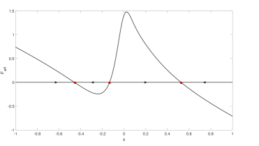
Figure 1: The effective force $F_{eff}(x):=\frac{\partial H_{eff}}{\partial\lambda}(0,x)$ for the model (46). Notice a pair of stable fixed points of the averaged dynamics separated by an unstable fixed point.

Euler-Lagrange equations associated with the effective action functional (18) are Hamilton’s with the Hamiltonian (30). Therefore, each solution lies on a constant energy surface $H_{eff}(\lambda,x)=E$. If there is a single slow variable, the trajectories coincide with constant energy surfaces. This allows one to determine a family of the most likely transition paths between the fixed points (the instanton trajectories) by building the contour plot of $H_{eff}$ numerically, see Fig. 2.

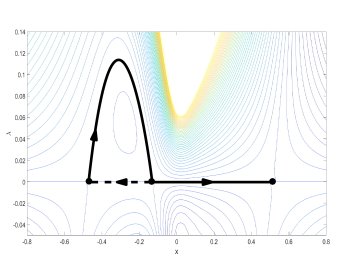
Figure 2: Contour lines of $H_{eff}$ for the model (46). The contour lines in the upper half plane serve as optimal trajectories for transitions between the stable fixed points in a finite time. The wide curve is the infinite-time optimal transition curve. The dashed segment marks the typical trajectory connecting the unstable and stable fixed points.

V Conclusions. Outlook

Motivated by hydrodynamic applications, we have considered a model with two-time scales, where the slow variable is driven by a quadratic function of a fast Gaussian process with rapidly decaying auto-correlations. A natural question of computing the probabilities of rare events in this model reduces to the computation of large-interval asymptotics for a certain Fredholm determinant. To the leading order, such a computation can be easily carried out using Widom’s theorem. To apply the resulting large deviation principle, we considered a special case of the fast field being a complex Ornstein-Ohlenbeck process with the the rotational component of the drift given by a linear function of the slow process. As it turns out, the average slow dynamics for such a model exhibits multiple equilibria, the transitions between which can be studied using large deviation theory.

There are many natural further questions to ask. Firstly, it should be a straightforward task to furnish a rigorous proof or provide a counter-example to the statement of the conjecture (18). Secondly, for the cases, when the fast process conditional on the value of the slow process is an Ornstein-Uhlenbeck process, it might be interesting to consider finite-$\epsilon$ corrections to the leading order answer. Albeit known, the sub-leading terms in the Widom asymptotic are only characterised as solutions to a certain matrix Wiener-Hopf integral equation. There is however a chance of finding these corrections rather more explicitly as solutions to time-dependent Riccatti equations derived in [17].

Finally, the model considered has the general structure of many equations of hydrodynamics, plasma dynamics, self-gravitating systems, wave turbulence or other physical system with quadratic couplings or interactions. It would therefore be extremely interesting to analyse metastability for such physical systems, in the presence of time scale separation, using the findings of the present paper.

Appendix A The derivation of (9)

In the calculation below we rely on the observation that the Gaussian process $Y(\cdot,x)$ with exponentially decaying autocorrelation function should be well approximated by a bounded process with a finite dependency range. In other words, we assume that there are a constants $C,\delta$: $Y^{T}(t,x)Y(t,x)\leq C$ for all $t,x$ and the processes $(Y(t,x))_{t<T}$ and $(Y(t,x))_{t>T+\delta}$ are independent for any $T\in\mathbb{R}$ .

To estimate a probability in terms of exponential moments, we follow the logic of Chernoff bound (the exponential version of Chebyshev’s inequality) and notice the following elementary inequality: for any $\lambda\in\mathbb{R}$,

$$\mathbbm{1}(x\in(y\!-\!\eta,y\!+\!\eta))\!\leq\!e^{\lambda(x-y)+\eta|\lambda|}\mathbbm{1}(x\in(y-\eta,y+\eta)).$$

The corresponding $n$-dimensional generalisation is

$$\mathbbm{1}(x\in b_{\eta}(y))\leq e^{\lambda^{T}(x-y)+\eta n||\lambda||_{\infty}}\mathbbm{1}(x\in b_{\eta}(y)),$$ (47)

where $\lambda,x,y\in\mathbb{R}^{n}$, $||\lambda||_{\infty}=\max_{1\leq\alpha\leq n}|\lambda_{\alpha}|$. Using (47),

$$\mathbb{P}\left[X(k\Delta t)\!\!\in\!\!b_{\eta}(x_{k}),1\!\leq\!k\!\leq\!P\right]\!\!=\!\!\mathbb{E}\!\!\left[\prod_{k=1}^{P}\!\!\mathbbm{1}\!\!\left(X(k\Delta t)\!\!\in\!\!b_{\eta}(x_{k})\right)\right]\!\!\leq\!\!\mathbb{E}\!\!\left[e^{\sum_{l=1}^{P}\left[\frac{\lambda_{l}^{T}}{\epsilon}(X(l\Delta t)-x_{l})+\eta n||\lambda_{l}||_{\infty}\right]}\!\!\prod_{k=1}^{P}\!\!\mathbbm{1}\!\!\left(X(k\Delta t)\!\!\in\!\!b_{\eta}(x_{k})\right)\right]~{}~{}~{}~{}$$ (48)

Next we need to calculate $X(k\Delta t)-x_{k}$ for each $k$ by solving (3) over the time interval $[(k-1)\Delta t,k\Delta t]$: Denote the right hand side of the equation for $\dot{X}(\tau)$ by $f(\tau/\epsilon,X(\tau))$. Our assumptions imply that both $||f||_{\infty}$ and $||\nabla_{2}f||_{\infty}$ are bounded by some constants, which will be denoted by $M_{0}$ and $M_{1}$ correspondingly. Expanding $f$ in Taylor series in the second argument one finds

$$\!\!\!\!\!\!\lambda^{T}\dot{X}(\tau)\!=\!\lambda^{T}\!f(\tau/\epsilon,x_{k-1})\!+\!\rho_{k},\tau\!\!\in\!\![(k\!-\!1)\Delta t,k\Delta t],$$ (49)

where $\rho_{k}=\lambda^{T}\nabla_{2}f(\tau/\epsilon,(1-c)x_{k-1}+cX(\tau))(X(\tau)-x_{k-1})$, for some $c\in(0,1)$. Here we used the mean value form of the remainder for the Taylor series. Using the bound $||\nabla_{2}f||_{\infty}\leq M_{1}$ and noticing that $\nabla_{2}f$ is an $n\times n$ matrix,

$$|\rho_{k}|\leq n^{2}||\lambda||_{\infty}M_{1}||X(\tau)-x_{k-1}||_{\infty}.$$ (50)

The estimate of the size of $X(\tau)-x_{k-1}$ uses the equation for $X$ once more:

$$||X(\tau)-x_{k-1}||_{\infty}$$

$$\leq\!\!||X(\tau)\!-\!X(\Delta t(k-1))||_{\infty}\!\!+\!\!||X(\Delta t(k-1))\!-\!x_{k-1}||_{\infty}$$

$$\leq\eta+||\int_{(k-1)\Delta t}^{\tau}d\tau^{\prime}f(\tau^{\prime}/\epsilon,X(\tau^{\prime}))||_{\infty}\leq\eta+\Delta tM_{0}.$$

The penultimate step uses the fact that the indicators under the sign of the expectation in (48) enforce the constraint $||X((k-1)\Delta t)-x_{k-1}||_{\infty}<\eta$; the last step uses the bound $||f||_{\infty}<M_{0}$. Putting it all together we find that

$$|\rho_{k}|\leq n^{2}||\lambda||_{\infty}(\eta+\Delta tM_{0})M_{1}.$$ (51)

Integrating (49) over the interval $[(k-1)\Delta t,k\Delta t]$ we conclude that

$$\lambda_{k}^{T}(X(k\Delta t)-x_{k})=\lambda_{k}^{T}(x_{k-1}-x_{k})$$

$$+\lambda_{k}^{T}\int_{(k-1)\Delta t}^{k\Delta t}\!\!\!\!\!\!\!\!\!\!\!\!d\tau f(\tau/\epsilon,x_{k-1})+\tilde{\rho}_{k},$$ (52)

where $||\tilde{\rho}_{k}||_{\infty}\leq||\lambda_{k}||_{\infty}(n\eta+n^{2}(\eta+\Delta tM_{0})M_{1}\Delta t)$. Notice the extra contribution to the error term coming from one more application of the bound $||X((k-1)\Delta t)-x_{k-1}||_{\infty}\leq\eta$. Substituting (52) into (48) and upper-bounding the product of the indicators by $1$, one arrives at the following intermediate result:

$$\mathbb{P}\left[X(k\Delta t)\in b_{\eta}(x_{k}),k=1,\ldots,P\right]$$

$$\leq e^{\sum_{k=1}^{P}\frac{\lambda_{k}^{T}}{\epsilon}\left(x_{k-1}-x_{k}\right)}$$

$$\mathbb{E}\left[\prod_{k=1}^{P}e^{\frac{\lambda_{k}^{T}}{\epsilon}\left(\int_{(k-1)\Delta t}^{k\Delta t}d\tau f(\tau/\epsilon,x_{k-1})+R_{k}\right)}\right],$$ (53)

where $R_{k}=||\lambda_{k}||_{\infty}(2n\eta+n^{2}(\eta+\Delta tM_{0})M_{1}\Delta t)$. It remains to approximate the expectation in (A) by the product of expectations. To this end we write

$$\lambda_{k}^{T}\int_{(k-1)\Delta t}^{k\Delta t}d\tau f(\tau/\epsilon,x_{k-1})=\epsilon\lambda_{k}^{T}\int_{(k-1)\Delta t/\epsilon}^{k\Delta t/\epsilon}\!\!\!\!d\tau f(\tau,x_{k-1})$$

$$=\epsilon\lambda_{k}^{T}\int_{(k-1)\Delta t/\epsilon+\delta}^{k\Delta t/\epsilon-\delta}d\tau f(\tau,x_{k-1})+E_{k},~{}~{}~{}~{}~{}~{}~{}~{}~{}$$ (54)

where the bound $||f||_{\infty}\leq M_{0}$ implies that $|E_{k}|\leq 2\epsilon n||\lambda_{k}||_{\infty}M_{0}\delta$. Crucially, notice that $f(\tau/\epsilon,x)$ depends on $Y(\tau/\epsilon,x)$ only. Therefore, the random variables $\epsilon\lambda_{k}^{T}\int_{(k-1)\Delta t/\epsilon-\delta}^{k\Delta t/\epsilon+\delta}d\tau f(\tau,x_{k-1})$, $1\leq k\leq P$ are mutually independent due to the finite dependency range $\delta$ of the process $Y$. Substituting (A) into (A) and exploiting the independence one finds

$$\mathbb{P}\left[X(k\Delta t)\in b_{\eta}(x_{k}),k=1,\ldots,P\right]$$

$$\leq e^{\sum_{k=1}^{P}\frac{\lambda_{k}^{T}}{\epsilon}\left(x_{k-1}-x_{k}+\tilde{R}_{k}\right)}\prod_{k=1}^{P}\mathbb{E}\left[e^{\lambda_{k}^{T}\int_{(k-1)\Delta t/\epsilon}^{k\Delta t/\epsilon}d\tau f(\tau,x_{k-1})}\right],$$

where $\tilde{R}_{k}=||\lambda_{k}||_{\infty}(4\epsilon nM_{0}\delta+2n\eta+n^{2}(\eta+\Delta tM_{0})M_{1}\Delta t)$. In the last expression we extended the integration interval back to $[(k-1)\Delta t,k\Delta t]/\epsilon$, which explains the doubling of the $\delta$-dependent contribution to error term. Finally, let us notice that the total error term $R(\epsilon,\Delta t,\eta):=\sum_{k=1}^{P}\tilde{R}_{k}$ has the following property:

$$\lim_{\mu\rightarrow 0}\lim_{\Delta t\rightarrow 0}\lim_{\epsilon\rightarrow 0}R(\epsilon,\Delta t,\mu\Delta t)=0.$$ (55)

The derivation of (9) is complete.

Appendix B The derivation of (III)

First of all let us explain what we mean by a ’nice’ set of functions $D$. To this end, we need to introduce one more notation. For $f\in C([0,T],\mathbb{R}^{n})$ let

$$B_{\eta}(f)\!\!=\!\!\{g\!\in\!C([0,t],\mathbb{R}^{n}):\!\!\!\!\!\!\!\!\!\!\!\sup_{\tau\in[0,t],1\leq\alpha\leq n}\!\!\!\!\!\!\!\!\!\!\!|f_{\alpha}(\tau)\!\!-\!\!g_{\alpha}(\tau)|\!<\!\eta\}.~{}~{}$$ (56)

This is an infinite-dimensional generalization of the hypercube $b_{\eta}$ introduced above. We say that the set $D$ is nice if for any $\eta>0$ we can find finitely many smooth functions $x^{(1)},x^{(2)},\ldots,x^{(M)}\in C([0,T],\mathbb{R}^{n}):$

$$D\subset\bigcup_{j=1}^{M}B_{\eta}(x^{(j)}).$$ (57)

In other words $D$ can be covered by finitely many hypercubes of any positive ‘linear size’ . Let $x^{(j)}_{k}=x^{(j)}(k\Delta t)$, $1\leq k\leq P$. Then

$$\mathbb{P}[X\in D]\stackrel{{\scriptstyle(\ref{appbincl})}}{{\leq}}\mathbb{P}\left[X\in\bigcup_{j=1}^{M}B_{\eta}(x^{(j)})\right]=\mathbb{P}[\exists j\leq M:X\in B_{\eta}(x^{(j)})]=\mathbb{P}\left[\exists j\leq M:X(\tau)\in b_{\eta}\left(x^{(j)}(\tau)\right),\tau\in[0,t]\right]$$

$$\leq\mathbb{P}\left[\exists j\leq M:X(k\Delta t)\in b_{\eta}\left(x^{(j)}_{k}\right),1\leq k\leq P\right]\stackrel{{\scriptstyle(*)}}{{\leq}}\sum_{k=1}^{M}\mathbb{P}\left[X(k\Delta t)\in b_{\eta}\left(x^{(j)}_{k}\right),1\leq k\leq P\right]$$

$$\leq M\max_{1\leq j\leq M}\mathbb{P}\left[\bigcap_{k=1}^{P}\left\{X(k\Delta t)\in b_{\eta}(x_{k}^{(j)})\right\}\right].$$

All of the above steps should be self-explanatory, let us just notice that the inequality $(*)$ is the union bound. Taking the logarithm of both sides of the derived inequality and using the bound (15) one finds

$$\epsilon\mathbb{P}[X\in D]\leq\epsilon\log M+\epsilon\max_{1\leq j\leq M}\log\mathbb{P}\left[\bigcap_{k=1}^{P}\left\{X(k\Delta t)\in b_{\eta}(x_{k}^{(j)})\right\}\right]\leq\epsilon\log M+\epsilon\sup_{x\in D}\log\mathbb{P}\left[\bigcap_{k=1}^{P}\left\{X(k\Delta t)\in b_{\eta}(x_{k})\right\}\right]$$

$$\stackrel{{\scriptstyle(\ref{step1})}}{{\leq}}\epsilon\log M+R+O(\epsilon P)+\sup_{x\in D}\left[\sum_{p=1}^{P}\Delta t\lambda_{p}^{T}\left(\frac{x_{p-1}-x_{p}}{\Delta t}-\nu x_{p-1}\right)-\frac{1}{2}\sum_{p=1}^{P}\Delta t\int_{\mathbb{R}}\frac{dk}{2\pi}\log\det\left(I-2\lambda_{p}^{T}M\tilde{C}(k,x_{p-1})\right)\right].$$

As a result,

$$\limsup_{\epsilon\rightarrow 0}\epsilon\mathbb{P}[X\in D]\leq\lim_{\epsilon\rightarrow 0}R\!+\!\sup_{x\in D}\sum_{p=1}^{P}\Delta t\left(\lambda_{p}^{T}\left(\frac{x_{p-1}\!-\!x_{p}}{\Delta t}\!-\!\nu x_{p-1}\right)\!-\!\frac{1}{2}\int_{\mathbb{R}}\frac{dk}{2\pi}\log\det\left(I\!-\!2\lambda_{p}^{T}M\tilde{C}(k,x_{p-1})\right)\right).~{}~{}$$ (58)

Finally, notice that the left-hand-side of (58) does not depend on $\Delta t,\eta$. Let $\lambda,x$ be a pair of $\mathbb{R}^{n}$-valued functions on $[0,t]$ such that

$$\lambda(k\Delta t)=\lambda_{k},~{}x(k\Delta t)=x_{k},1\leq k\leq P.$$

Setting $\eta=\mu\Delta t$, applying $\lim_{\mu\rightarrow 0}\lim_{\Delta t\rightarrow 0}$ to both sides of (58) and using the property (11) of the error term one arrives at (III).

Appendix C Lower bound on $\log\mathbb{P}[X\in D]$

For the lower bound, let us take the pair $x,\lambda\in C([0,t],\mathbb{R}^{n})$ to be the solution to the Euler-Lagrange equations describing the critical points of (18) and assume that the solution is unique and smooth. The boundedness of the right hand side of the equation for $\dot{x}$ means that there is $M_{2}>0$ such that $||\dot{x}(t)||_{\infty}<M_{2}$ for all $t\in[0,t]$.

Let us fix $\Delta t>0$. Using the above bound on $\dot{x}$ and the bound $||f||_{\infty}<M_{0}$ discussed in the text above (49), it is easy to establish the following: if $X(t)\in b_{\eta}(x(t))$ at some time $t$, then for all $\tau\in[t,t+\Delta t]$,

$$||X(\tau)-x(\tau)||_{\infty}\leq\eta+(M_{0}+M_{2})\Delta t.$$ (59)

Let $x_{k}=x(k\Delta t),\lambda_{k}=\lambda(k\Delta t)$, $1\leq k\leq P$, where $P=\lfloor\frac{t}{\Delta t}\rfloor$. Choose $\rho>0$: $B_{\rho}(x)\subset D$. Then

$$\mathbb{P}[X\in D]\geq\mathbb{P}[X\in B_{\rho}(x)]$$ (60)

$$\geq\mathbb{P}[X(k\Delta t)\in b_{\eta}(x_{k}),1\leq k\leq P]$$

provided $\eta>0$ and $\Delta t>0$ are such that $\eta+(M_{0}+M_{2})\Delta t<\rho$: given such a choice, the estimate (59) implies the inclusion of events $\cap_{k=1}^{P}\{X(k\Delta t)\in b_{\eta}(x_{k})\}\subset\{X\in B_{\rho}(x)\}$, which leads to the claimed inequality in (60).

Following the steps which led to (52), one finds

$$\!\!\!\!\!\!\!X_{k}\!\!-\!\!X_{k-1}\!\!=\!\!\int_{(k-1)\Delta t}^{k\Delta t}\!\!\!\!\!\!\!\!\!\!\!\!f(\tau/\epsilon,x_{k-1})d\tau+V_{k},$$ (61)

where $X_{k}:=X(k\Delta t)$ and $||V_{k}||_{\infty}\leq nM_{1}(\eta+\Delta tM_{0})\Delta t$. Let

$$F^{(\epsilon)}_{k}=\int_{(k-1)\Delta t+\epsilon\delta}^{k\Delta t}f(\tau/\epsilon,x_{k-1})d\tau.$$

By the finite dependency assumption the random variables $\left(F^{(\epsilon)}_{k}\right)_{k\geq 1}$ are independent. Define $F_{k-1}:=F_{k-1}^{(0)}$. Then right hand side of (61) is equal to $F_{k-1}+V_{k}$. Notice the following elementary inequality:

$$\mathbbm{1}(X+v\in b_{\eta}(x))\geq\mathbbm{1}(X\in b_{\eta-||v||_{\infty}}(x)).$$ (62)

The right hand side is non-zero provided $||v||_{\infty}<\eta$. The following estimate is based on (60), the independence of $(F_{k}^{(\epsilon)})_{k\geq 1}$, the inequality (62) and the tower property of conditional probabilities:

$$\mathbb{P}[X\in D]\geq\mathbb{P}[X\in B_{\rho}(x)]\geq\mathbb{E}[\prod_{k=1}^{P}\mathbbm{1}(X_{k}\in b_{\eta}(x_{k}))]=\mathbb{E}\left[\mathbb{E}\left[\prod_{k=1}^{P}\mathbbm{1}(X_{k}\in b_{\eta}(x_{k}))\bigg{|}(Y_{\tau})_{0\leq\tau\leq(P-1)\Delta t/\epsilon}\right]\right]$$

$$=\mathbb{E}\left[\prod_{k=1}^{P-1}\mathbbm{1}(X_{k}\in b_{\eta}(x_{k}))\mathbb{E}\left[\mathbbm{1}(X_{P}\in b_{\eta}(x_{P}))\bigg{|}(Y_{\tau})_{0\leq\tau\leq(P-1)\Delta t/\epsilon}\right]\right]=\mathbb{E}\left[\prod_{k=1}^{P-1}\mathbbm{1}(X_{k}\in b_{\eta}(x_{k}))\right.$$

$$\left.\mathbb{E}\left[\mathbbm{1}(X_{P-1}+F_{P}^{(\epsilon)}+v\in b_{\eta}(x_{P}))\bigg{|}(Y_{\tau})_{0\leq\tau\leq(P-1)\Delta t/\epsilon}\right]\right]\geq\min_{y_{P-1}\in b_{\eta}(x_{P-1})}\mathbb{E}\left[\prod_{k=1}^{P-1}\mathbbm{1}(X_{k}\in b_{\eta}(x_{k}))\right.$$

$$\left.\mathbb{E}\left[\mathbbm{1}(y_{P-1}+F_{P}^{(\epsilon)}+v\in b_{\eta}(x_{P}))\bigg{|}(Y_{\tau})_{0\leq\tau\leq(P-1)\Delta t/\epsilon}\right]\right]=\min_{y_{P-1}\in b_{\eta}(x_{P-1})}\mathbb{E}\left[\prod_{k=1}^{P-1}\mathbbm{1}(X_{k}\in b_{\eta}(x_{k}))\right]$$

$$\mathbb{E}\left[\mathbbm{1}(y_{P-1}+F_{P}^{(\epsilon)}+v\in b_{\eta}(x_{P}))\right]\geq\prod_{k=1}^{P}\min_{y_{k-1}\in b_{\eta}(x_{k-1})}\mathbb{E}\left[\mathbbm{1}(y_{k-1}+F_{k}^{(\epsilon)}+v\in b_{\eta}(x_{k}))\right]$$

$$=\prod_{k=1}^{P}\min_{y_{k-1}\in b_{\eta}(x_{k-1})}\mathbb{E}\left[\mathbbm{1}(y_{k-1}+F_{k}+w\in b_{\eta}(x_{k}))\right]\geq\prod_{k=1}^{P}\min_{y_{k-1}\in b_{\eta}(x_{k-1})}\mathbb{E}\left[\mathbbm{1}(y_{k-1}+F_{k}\in b_{\eta-r}(x_{k}))\right]$$ (63)

Here $v$ and $w$ are a shorthand notation for random errors satisfying deterministic bounds on their norms, $||v||_{\infty}\leq nM_{1}(\eta+\Delta tM_{0})\Delta t+\epsilon M_{0}\delta$, $||w||_{\infty}\leq nM_{1}(\eta+\Delta tM_{0})\Delta t+2\epsilon M_{0}\delta$, and $r=nM_{1}(\eta+\Delta tM_{0})\Delta t+2\epsilon M_{0}\delta$.

The following steps are standard in the context of the theory of large deviations: let $\eta^{\prime}=\eta-r$. Then notice that

$$\mathbb{E} \left[\mathbbm{1}\left(F_{k}\in b_{\eta}(x_{k}-y_{k-1})\right)\right]=\mathbb{E}\left[e^{-\frac{1}{\epsilon}\lambda_{k}^{T}F_{k}}e^{\frac{1}{\epsilon}\lambda_{k}^{T}F_{k}}\mathbbm{1}\left(F_{k}\in b_{\eta^{\prime}}(x_{k}-y_{k-1})\right)\right]\geq e^{-\frac{\lambda_{k}(x_{k}-y_{k-1})+n||\lambda_{k}||_{\infty}\eta^{\prime}}{\epsilon}}$$ (64)

$$\mathbb{E} \left[e^{\frac{1}{\epsilon}\lambda_{k}^{T}F_{k}}\mathbbm{1}\left(F_{k}\in b_{\eta^{\prime}}(x_{k}-y_{k-1})\right)\right]=e^{-\frac{\lambda_{k}(x_{k}-y_{k-1})+n||\lambda_{k}||_{\infty}}{\epsilon}}\mathbb{E}\left[e^{\frac{1}{\epsilon}\lambda_{k}^{T}F_{k}}\right]\mathbb{E}^{(\lambda_{k})}\left[\mathbbm{1}\left(F_{k}\in b_{\eta^{\prime}}(x_{k}-y_{k-1})\right)\right],$$

where

$$\mathbb{E}^{(\lambda_{k})}[\bullet]:=\frac{\mathbb{E}[e^{\frac{1}{\epsilon}\lambda_{k}^{T}F_{k}}\bullet]}{\mathbb{E}\left[e^{\frac{1}{\epsilon}\lambda_{k}^{T}F_{k}}\right]},$$

is the expectation with respect to the probability measure tilted by the exponential factor $e^{\frac{1}{\epsilon}\lambda_{k}^{T}F_{k}}$. The derivation of (63,64) did not use any assumptions about the sequence $(\lambda_{1},\ldots\lambda_{P})$. Now let us choose the sequence in such a way that

$$\lim_{\epsilon\rightarrow 0}\mathbb{E}^{(\lambda_{k})}[F_{k}]=x_{k}-y_{k-1},~{}1\leq k\leq P,$$ (65)

which coincides with the discretised version of the Euler-Lagrange equations $\delta S_{eff}/\delta\lambda(\tau)=0,~{}0<\tau<t$ if $y_{k}=x_{k}$ for all $k$’s. Equivalently,

$$\!\!\!\!\frac{\partial}{\partial\lambda_{k}}\lim_{\epsilon\rightarrow 0}\!\epsilon\!\log\mathbb{E}[e^{\frac{1}{\epsilon}\lambda_{k}^{T}F_{k}}]\!=\!x_{k}\!-\!y_{k-1},1\leq k\leq P.$$ (66)

Recall that an explicit formula derived with the help of Widom’s theorem shows that $\lim_{\epsilon\rightarrow 0}\epsilon\log\mathbb{E}[e^{\frac{1}{\epsilon}\lambda_{k}^{T}F_{k}}]$ is finite, see (12) and (14). Calculating the second $\lambda$-derivative of $\log\mathbb{E}[e^{\frac{1}{\epsilon}\lambda^{T}F_{k}}]$ one finds that

$$\lim_{\epsilon\rightarrow 0}\mbox{Cov}^{(\lambda_{k})}[F_{k}]=\lim_{\epsilon\rightarrow 0}\epsilon^{2}\partial_{\lambda}\otimes\partial_{\lambda}\log\mathbb{E}[e^{\frac{1}{\epsilon}\lambda^{T}F_{k}}]=0.$$ (67)

Expressions (65), (67) and Chebyshev’s inequality imply that

$$\lim_{\epsilon\rightarrow 0}\mathbb{E}^{(\lambda_{k})}\left[\mathbbm{1}\left(F_{k}\in b_{\eta^{\prime}}(x_{k}-y_{k-1})\right)\right]=1.$$

Using this observation in (63, 64) one finds that

$$\liminf_{\epsilon\rightarrow 0}\epsilon\log\mathbb{P}[X\in D]$$ (68)

$$\geq \sum_{k=1}^{P}\min_{y_{k-1}\in b_{\eta}(x_{k-1})}\left\{\left(\lambda_{k}^{T}(y_{k-1}-x_{k})-n||\lambda_{k}||_{\infty}\eta^{\prime\prime}\right)\right.$$

$$+ \left.\lim_{\epsilon\rightarrow 0}\epsilon\log\mathbb{E}\left[e^{\frac{1}{\epsilon}\lambda_{k}^{T}F_{k}}\right]\right\},$$

provided the sequence $(\lambda_{k})$ solves (65). Here

$$\eta^{\prime\prime}=\eta^{\prime}\mid_{\epsilon=0}=\eta-r\mid_{\epsilon=0}=\eta-nM_{1}(\eta+\Delta tM_{0})\Delta t.$$

As the right hand side of (68) does not depend on $\eta$ and $\Delta t$, one can set $\eta=a(\Delta t)^{\mu}$, where $a>0$ and $\mu>1$ and take the limit $\Delta t\rightarrow 0$. In the limit, using that $y_{k}\in b_{\eta}(x_{k})$, one finds that the system of equations (66) becomes

$$\!\!\!\!\frac{\partial}{\partial\lambda(\tau)}\lim_{\Delta t,\epsilon\rightarrow 0}\!\frac{\epsilon}{\Delta t}\!\log\mathbb{E}[e^{\frac{1}{\epsilon}\lambda_{k}^{T}F_{k}}]\mid_{k=\frac{\tau}{\Delta t}}\!=\!\dot{x}(\tau),~{}\tau\in[0,t].$$

Due to (12), (14), the above equation coincides with the Euler-Lagrange equation $\frac{\delta S_{eff}}{\delta\lambda(\tau)}=0$, where $S_{eff}$ is given by (18). The bound (68) becomes

$$\!\!\!\!\!\liminf_{\epsilon\rightarrow 0}\epsilon\log\mathbb{P}[X\in D]\geq\int_{0}^{t}d\tau\bigg{(}-\lambda^{T}(\tau)\cdot{x}(\tau)$$ (69)

$$+\lim_{\Delta t\rightarrow 0}\lim_{\epsilon\rightarrow 0}\frac{\epsilon}{\Delta t}\log\mathbb{E}\left[e^{\frac{1}{\epsilon}\lambda_{k}^{T}F_{k}}\right]\big{|}_{k\Delta t=\tau}\bigg{)},$$

where the functions $\lambda,x$ solve the Euler-Lagrange equations associated with the effective action functional $S_{eff}$. Furthermore, the right hand side of (69) coincides with the effective action functional (18). Therefore, by the assumed uniqueness of the solution to the Euler Lagrange equaitons, the right hand side of (69) must coincide with (III). The lower bound is derived.

Appendix D Widom’s theorem

To the best of our knowledge, a proof of Widom’s theorem has never been published. In [21] Widom simply formulates the theorem, states that it can be easily verified by taking the continuous limit of the corresponding statement for large Toeplitz matrices and then moves on to the main topic of the paper: the asymptotic of Fredholm determinants for operators acting on spaces of functions of several variables. Thus there is a gap in the story, which we partially fill in the present Appendix by deriving (14). In our proof we use the probabilistic method developed in the original paper by Kac [25].

Theorem. Let $K:\mathbb{R}\rightarrow\mathbb{R}^{N\times N}$ be an $N\times N$ matrix-valued function of one variable. Assume that $K$ is even ($K(t)=K(-t)$, for any $t\in\mathbb{R}$) and non-negative ($K_{ij}(t)\geq 0$ for any $t\in\mathbb{R}$ and $1\leq i,j\leq N$). Assume in addition that

$$\int_{\mathbb{R}}|t|K(t)dt<\infty,$$ (70)

$$\int_{\mathbb{R}}\sum_{k=1}^{N}K_{ki}\leq 1,~{}1\leq i\leq N.$$ (71)

The function $K$ can be regarded as a kernel of an integral operator $\hat{K}$ acting on square-integrable functions from $\mathbb{R}$ to $\mathbb{R}^{N}$,

$$f\mapsto\hat{K}f(t)=\int_{\mathbb{R}}d\tau K(t-\tau)f(\tau),~{}t\in\mathbb{R}.$$ (72)

Then there is $\lambda_{max}>0$ such that for any $\lambda:|\lambda|<\lambda_{max}$ the Fredholm determinant $\text{Det}(I-\lambda\hat{K}_{T})$ exists and

$$\log\text{\text{Det}}(I-\lambda\hat{K}_{T})=\!\!T\!\!\int_{\mathbb{R}}\frac{dk}{2\pi}\log\det(1-\lambda\tilde{K}(k))$$

$$+O(T^{0}),$$ (73)

where $\hat{K}_{T}$ is the restriction of $\hat{K}$ to functions on $[0,T]$ and

$$\tilde{K}(k)=\int_{\mathbb{R}}dxe^{-ikx}K(x),~{}k\in\mathbb{R}.$$ (74)

Let us sketch the proof of the theorem using, as we already mentioned, the probabilistic method used in [25] to prove a continuous version of Szegö’s formula for the asymptotics of Toeplitz determinants. For a sufficiently small $|\lambda|$ we can calculate the Fredholm determinant using the trace-log formula,

$$\log\text{Det}(I-\lambda\hat{K}_{T})=-\sum_{n=1}^{\infty}\frac{1}{n}\lambda^{n}\text{Tr}\hat{K}_{T}^{n},$$ (75)

where

$$\text{Tr}\hat{K}_{T}^{n}=\int_{[0,T]^{n}}dx_{1}dx_{2}\ldots dx_{n}$$

$$\text{tr}K(x_{1}-x_{2})K(x_{2}-x_{3})\ldots K(x_{n}-x_{1}).$$

Using the cyclic property of trace and the fact that the function $K$ is even, we find

$$\frac{d}{dT}\text{Tr}\hat{K}_{T}^{n}=n\int_{[0,T]^{n}}dx_{2}dx_{3}\ldots dx_{n}$$

$$\text{tr}K(-x_{2})K(x_{2}-x_{3})\ldots K(x_{n-1}-x_{n})K(x_{n}).$$ (76)

Consider the following discrete time Markov chain $\{X_{n},S_{n}\}_{n\geq 0}$ on the state space $\mathbb{R}\times\{1,2,\ldots,N\}$:

1. $(X_{0},S_{0})\sim(\delta_{0},U_{N})$, where $U_{N}$ is the uniform distribution on $\{1,2,\ldots,N\}$.

2. At each time step, the transition $(x,i)\rightarrow(y,k)$ happens with probability $K_{ki}(y-x)dy$.

Notice that this is a Markov chain with killing, the survival probability when transitioning from state $(x,i)$ is $g_{i}(x):=\sum_{k=1}^{N}\int_{\mathbb{R}}K_{ki}(y-x)dy\leq 1$. Examining the expression (76) for the derivative of the trace of the $n$-th power of $\hat{K}$, we see that it can be interpreted as the following expectation with respect to the law of the chain $\{X_{n},S_{n}\}_{n\geq 0}$:

$$\!\!\!\!\!\!\frac{d}{dT}\text{Tr}\hat{K}_{T}^{n}\!=\!Nn\mathbb{E}\left(\mathbbm{1}(X_{n}\in d0)\mathbbm{1}(S_{n}\!=\!S_{0})\mathbbm{1}(\tau\!=\!n)\right),$$ (77)

where $\tau$ is the first exit time of the chain from the interval $(0,T)\times\{1,2,\ldots,N\}$. To derive the above expression we exploited the identity $\mathbbm{1}(X_{n}\in d0)\mathbbm{1}(\tau\geq n)=\mathbbm{1}(X_{n}\in d0)\mathbbm{1}(\tau=n)$. Substituting (77) into (76) and then (75), we find that

$$\frac{d}{dT}\log\text{Det}(I\!-\!\lambda\hat{K}_{T})\!=\!-N\mathbb{E}\left(\lambda^{\tau}\mathbbm{1}(X_{\tau}\in d0)\mathbbm{1}(S_{\tau}=S_{0})\right)$$

$$=-N\mathbb{E}\left(\lambda^{\tau_{0}}\mathbbm{1}(X_{\tau_{0}}\in d0)\mathbbm{1}(M_{\tau_{0}}<T)\mathbbm{1}(S_{\tau_{0}}=S_{0})\right),$$

where $\tau_{0}$ is the first exit time from $(0,\infty)\times\{1,2,\ldots,N\}$, $M_{\tau_{0}}=\max_{1\leq n<\tau_{0}}(X_{n})$. As $\log\det(I-\lambda\hat{K}_{0})=0$, we can integrate the last expression to find

$$\log\text{Det}(I-\lambda\hat{K}_{T})$$

$$=-N\mathbb{E}\left(\lambda^{\tau_{0}}\mathbbm{1}(X_{\tau_{0}}\in d0)(T-M_{\tau_{0}})_{+}\mathbbm{1}(S_{\tau_{0}}=S_{0})\right),$$

where $(x)_{+}:=\max(x,0)$. Noticing that $T-(T-M)_{+}=\min(T,M)$, we can re-arrange the above expression as follows:

$$\log\text{Det}(I-\hat{K}_{T})=-NT\mathbb{E}\left(\lambda^{\tau_{0}}\mathbbm{1}(X_{\tau_{0}}\in d0)\mathbbm{1}(S_{\tau_{0}}=S_{0})\right)$$

$$+N\mathbb{E}\left(\lambda^{\tau_{0}}\mathbbm{1}(X_{\tau_{0}}\in d0)\min(T,M_{\tau_{0}})\mathbbm{1}(S_{\tau_{0}}=S_{0})\right),$$

This is an exact expression for the Fredholm determinant as an expectation with respect to the law of the Markov chain we defined. In many cases it allows for an efficient computation of the large-$T$ expansion of the Fredholm determinant using purely probabilistic methods. For us it is sufficient to check that $\lim_{T\rightarrow\infty}\min(T,M_{\tau_{0}})=M_{\tau_{0}}$, which implies that

$$\log\text{Det}(I\!-\!\lambda\hat{K}_{T}) = \!-NT\mathbb{E}\left(\lambda^{\tau_{0}}\!\mathbbm{1}(X_{\tau_{0}}\!\in\!d0)\mathbbm{1}(S_{\tau_{0}}=S_{0})\right)$$ (78)

$$+ O(T^{0}).$$

To calculate the expectation entering the leading term we use the following combinatorial lemma (see e. g. [26], volume $2$): Let $(0,R_{1},R_{1}+R_{2},\ldots,R_{1}+R_{2}+\ldots+R_{n-1},0)$ be the first $n$ $\mathbb{R}$-projections of the states of the chain with $\tau_{0}=n$. Then

$$\sum_{p=0}^{n-1}\prod_{k=1}^{n-1}\mathbbm{1}(R_{1+p}+R_{2+p}+\ldots+R_{k+p}>0)$$

$$=1~{}\text{a. s.},~{}0\leq p\leq n-1.$$ (79)

The addition of subscripts in the above formula should be understood modulo $n$. The above statement is very general and relies only on the absence of atoms in the transition probabilities $K(y-x)dy$.

In this case, for any sequence $(0,R_{1},R_{1}+R_{2},\ldots,R_{1}+R_{2}+\ldots+R_{n-1},0)$, its graph will almost surely have a unique global minimum, so there will be a unique cyclic permutation $(0,R_{1+p},R_{1+p}+R_{2+p},\ldots,R_{1+p}+R_{2+p}+\ldots+R_{n-1+p},0)$, whose graph will stay positive between times $1$ and $n-1$. Then

$$N\mathbb{E}\left(\lambda^{\tau_{0}}\mathbbm{1}(X_{\tau_{0}}\in d0)\mathbbm{1}(S_{\tau_{0}}=S_{0})\right)=N\sum_{n=1}^{\infty}\lambda^{n}\mathbb{E}\left(\mathbbm{1}(X_{\tau_{0}}\in d0)\mathbbm{1}(S_{\tau_{0}}=S_{0})\mathbbm{1}(\tau_{0}=n)\right)$$ (80)

$$= \sum_{n=1}^{\infty}\lambda^{n}\int_{\mathbb{R}^{n}}dr_{1}\ldots dr_{n}\text{tr}(K(r_{1})\ldots K(r_{n}))\delta(r_{1}+\ldots+r_{n})\prod_{k=1}^{n-1}\mathbbm{1}(r_{1}+\ldots+r_{k}>0)$$

$$= \sum_{n=1}^{\infty}\frac{\lambda^{n}}{n}\int_{\mathbb{R}^{n}}dr_{1}\ldots dr_{n}\text{tr}(K(r_{1})\ldots K(r_{n}))\delta(r_{1}+\ldots+r_{n})\sum_{p=0}^{n-1}\prod_{k=1}^{n-1}\mathbbm{1}(r_{1+p}+\ldots+r_{k+p}>0)$$

$$= \sum_{n=1}^{\infty}\frac{\lambda^{n}}{n}\int_{\mathbb{R}^{n}}dr_{1}\ldots dr_{n}\text{tr}(K(r_{1})\ldots K(r_{n}))\delta(r_{1}+\ldots+r_{n})$$

$$= \sum_{n=1}^{\infty}\frac{\lambda^{n}}{n}\int_{\mathbb{R}}\frac{dk}{2\pi}\int_{\mathbb{R}^{n}}dr_{1}\ldots dr_{n}e^{-ik(r_{1}+\ldots+r_{n})}\text{tr}(K(r_{1})\ldots K(r_{n}))$$

$$= \sum_{n=1}^{\infty}\frac{\lambda^{n}}{n}\int_{\mathbb{R}}\frac{dk}{2\pi}\text{tr}(\tilde{K}(k_{1})\ldots\tilde{K}(k_{n}))=-\int_{\mathbb{R}}\frac{dk}{2\pi}\log\det(I-\lambda\tilde{K}(k)).$$

The third inequality is the symmetrisation of the integrand with respect to all cycling permutations, the fourth inequality is due to the combinatorial lemma (79). Substituting (80) into (78), we arrive at the statement (73) of Widom’s theorem.

Remarks.

1. In [21] Widom presents a stronger version of the above statement which characterises the $O(T^{0})$ term fully. For the current paper we only need the leading term.

2. The actual statement of Widom’s theorem does not require the positivity of the kernel. In fact, all steps of the proof presented below go through for signed kernels as well, but the probabilistic intuition guiding these steps is lost. See also [25] for similar remarks about the original proof of Szegő’s theorem by Marc Kac.

3. It is possible to give an alternative derivation of (14) based on the re-summation of the cumulant expansion for the expectation of a quadratic function of a Gaussian process. The downside of such a derivation is difficulty in controlling the sub-leading terms.

References

- Bertini et al. [2015] L. Bertini, A. De Sole, D. Gabrielli, G. Jona-Lasinio, and C. Landim, Macroscopic fluctuation theory, Reviews of Modern Physics 87, 593 (2015).
- Saito and Dhar [2011] K. Saito and A. Dhar, Generating function formula of heat transfer in harmonic networks, Physical Review E 83, 041121 (2011).
- Lifshitz and Pitaevskii [1981] E. M. Lifshitz and L. P. Pitaevskii, Physical kinetics (Course of theoretical physics, Oxford: Pergamon Press, 1981, 1981).
- Nicholson [1983] D. Nicholson, Introduction to plasma theory (Wiley, New-York, 1983).
- Binney and Tremaine [1987] J. Binney and S. Tremaine, Galactic dynamics (Princeton, NJ, Princeton University Press, 1987, 747 p., 1987).
- Bouchet et al. [2013] F. Bouchet, C. Nardini, and T. Tangarife, Kinetic theory of jet dynamics in the stochastic barotropic and 2d navier-stokes equations, J. Stat. Phys. 153, 572 (2013).
- Nazarenko [2011] S. Nazarenko, Wave turbulence, Vol. 825 (Springer Science & Business Media, 2011).
- Landau and Lifshitz [1976] L. D. Landau and E. M. Lifshitz, Mechanics: Volume 1, Vol. 1 (Butterworth-Heinemann, 1976).
- Pavliotis and Stuart [2008] G. Pavliotis and A. Stuart, Multiscale methods: averaging and homogenization (Springer Science & Business Media, 2008).
- Freidlin et al. [2012] M. I. Freidlin, J. Szücs, and A. D. Wentzell, Random perturbations of dynamical systems, Vol. 260 (Springer Science & Business Media, 2012).
- Bouchet and Simonnet [2009] F. Bouchet and E. Simonnet, Random Changes of Flow Topology in Two-Dimensional and Geophysical Turbulence, Physical Review Letters 102, 094504 (2009).
- Bouchet et al. [2019] F. Bouchet, J. Rolland, and E. Simonnet, Rare event algorithm links transitions in turbulent flows with activated nucleations, Physical Review Letters 122, 074502 (2019).
- Freidlin [1978] M. I. Freidlin, The averaging principle and theorems on large deviations, Russian Mathematical Surveys 33, 117 (1978).
- Veretennikov [2000] A. Y. Veretennikov, On large deviations for sdes with small diffusion and averaging, Stochastic Processes and their Applications 89, 69 (2000).
- Kifer [1992] Y. Kifer, Averaging in dynamical systems and large deviations, Inventiones Mathematicae 110, 337 (1992).
- Kifer [2004] Y. Kifer, Averaging principle for fully coupled dynamical systems and large deviations, Ergodic Theory and Dynamical Systems 24, 847 (2004).
- Bouchet et al. [2016] F. Bouchet, T. Grafke, T. Tangarife, and E. Vanden-Eijnden, Large deviations in fast–slow systems, Journal of Statistical Physics 162, 793 (2016).
- Bouchet et al. [2014] F. Bouchet, J. Laurie, and O. Zaboronski, Langevin dynamics, large deviations and instantons for the quasi-geostrophic model and two-dimensional euler equations, Journal of Statistical Physics 156, 1066 (2014).
- Feliachi and Bouchet [2021] O. Feliachi and F. Bouchet, Dynamical large deviations for homogeneous systems with long range interactions and the balescu–guernsey–lenard equation, arXiv preprint arXiv:2105.05644 (2021).
- Martin et al. [1973] P. C. Martin, E. Siggia, and H. Rose, Statistical dynamics of classical systems, Physical Review A 8, 423 (1973).
- Widom [1980] H. Widom, Szegö’s limit theorem: the higher-dimensional matrix case, Journal of Functional Analysis 39, 182 (1980).
- Durrett [2019] R. Durrett, Probability: theory and examples, Vol. 49 (Cambridge university press, 2019).
- Note [1] It is the absence of error estimates associated with this approximation which makes our present discussion non-rigorous.
- Note [2] A mathematician would say that is a totally bounded subset of the complete space and is therefore compact.
- Kac et al. [1954] M. Kac et al., Toeplitz matrices, translation kernels and a related problem in probability theory, Duke Mathematical Journal 21, 501 (1954).
- Feller [2008] W. Feller, An introduction to probability theory and its applications, vol 2 (John Wiley & Sons, 2008).