D. Rindori
Università di Firenze and INFN Sezione di Firenze
Via G. Sansone 1, Sesto Fiorentino, I-50019 Florence, Italy
L. Tinti
Institut für Theoretische Physik, Johann Wolfgang Goethe-Universität
Max-von-Laue-Str. 1, D-60438 Frankfurt am Main, Germany
Instytut Fizyki,
Uniwersytet Jana Kochanowskiego w Kielcach
ul. Uniwersytecka 7,
PL 25-406 Kielce, Poland
F. Becattini
Università di Firenze and INFN Sezione di Firenze
Via G. Sansone 1, Sesto Fiorentino, I-50019 Florence, Italy
D.H. Rischke
Institut für Theoretische Physik, Johann Wolfgang Goethe-Universität
Max-von-Laue-Str. 1, D-60438 Frankfurt am Main, Germany
Helmholtz Research Academy Hesse for FAIR, Campus Riedberg, Max-von-Laue-Str. 12, D-60438 Frankfurt am Main, Germany
Abstract
We study a relativistic fluid with longitudinal boost invariance in a quantum-statistical
framework as an example of a solvable non-equilibrium problem. For the free quantum field, we calculate
the exact form of the expectation values of the stress-energy tensor and the entropy current. For the
stress-energy tensor, we find that a finite value can be obtained only by subtracting the vacuum
of the density operator at some fixed proper time . As a consequence, the stress-energy
tensor acquires non-trivial quantum corrections to the classical free-streaming form.
I Introduction
Spurred by a successful description of experimental data in high-energy nuclear collisions, relativistic hydrodynamics
has recently made major progress, both regarding its theoretical foundations as well as its phenomenological applications.
Lately, the quantum-statistical foundations of relativistic hydrodynamics have attracted a great deal of
attention betaframe ; hayata ; kaminski ; tinti ; calabrese , in particular to describe quantum phenomena in relativistic
fluids such as chirality chirality and polarization polarization . In a quantum-statistical framework, hydrodynamic
quantities, such as the stress-energy tensor and conserved currents, are the expectation values of the corresponding quantum operators with respect to a suitable statistical (or density) operator :
(1)
where the subscript “” implies renormalization of the otherwise divergent expectation value.
In general, the form of the stress-energy tensor and the currents crucially depends on the density operator. Exact expressions are known only in a few
cases, including the familiar global thermodynamic equilibrium and, as a recent development, global thermodynamic equilibrium
with rotation and acceleration. However, no exact form is known in local thermodynamic equilibrium,
which is defined by zubarev ; weert ; betaframe ; hayata :
(2)
where is a four-temperature field [equal to the four-velocity divided by the temperature ],
is a scalar field [equal to the ratio of the chemical potential associated with the conserved
current and the temperature]. The hypersurface is a three-dimensional space-like hypersurface, on
which local equilibrium is defined. The calculation of expectation values of operators using Eq. (2)
can be performed only in the hydrodynamic limit of slowly varying fields betaframe . For the stress-energy
tensor, the leading-order term coincides with the familiar perfect-fluid expression. Beyond this approximation,
quantum corrections appear, which have been estimated by means of a perturbative expansion only in the global-equilibrium case becaquant .
Recently, S. Akkelin Akkelin1 ; Akkelin2 has derived an exact solution of a particular non-equilibrium problem, a
free neutral scalar field with the density operator:
(3)
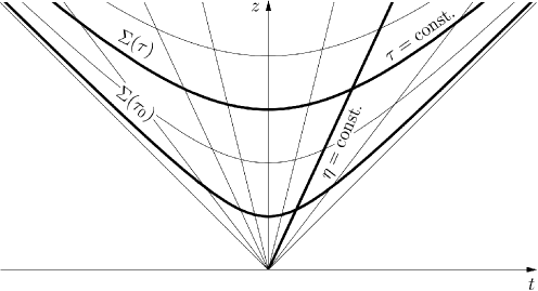
with being a proper-time hyperbola in the future light-cone in two dimensions
(see Fig. 1) and the four-velocity field coinciding with the unit vector perpendicular
to . The density operator (3) is invariant under longitudinal boosts, a symmetry
which has been often used to study general features of relativistic hydrodynamics problems. Lately,
longitudinal boost-invariant solutions have been studied in the context of spin-hydrodynamics florkowski
and magneto-hydrodynamics rischke1 ; rischke2 ; qunwang .
Figure 1: Two-dimensional section of the future light cone. Curves of constant Milne time
are hyperbolae, while curves of constant space-time rapidity are lines through the origin.
The thicker hyperbolae are two-dimensional sections of the three-dimensional hypersurfaces
and at constant and constant , respectively.
This symmetry and the solution found in Ref. Akkelin1 also offers a special opportunity to explore in
detail some essential features of quantum relativistic hydrodynamics in a non-equilibrium situation and, in
particular, to determine the pure quantum corrections to classical hydrodynamics and kinetic equations, including
those to the stress-energy tensor and to the entropy current. In other words, this solution provides a benchmark
test of a relativistic quantum fluid.
In this work, we extend the results of Ref. Akkelin1 and study the stress-energy
tensor with longitudinal boost-invariant symmetry. We find that, even for the simplest case of a free
scalar field, there are relevant quantum corrections related to its renormalization by subtraction
of the vacuum expectation value. Indeed, while the traditional vacuum of the field, expanded in plane
waves, the so-called Minkowski vacuum, fails to provide a finite energy density, the subtraction of the vacuum
expectation value with respect to the vacuum of the density operator does. Conversely, for the entropy current,
no significant quantum correction is found.
This paper is organized as follows.
We will start in Sec. II with a review of the density-operator approach in relativistic
quantum-statistical mechanics with special emphasis on symmetry considerations.
In Sec. III we will specialize to the symmetry of concern for this work, that is boost invariance.
As underlying quantum field theory, in Sec. IV we will present the field theory of the free neutral
scalar field in the future light cone, including a diagonalization of the density operator.
This will put us in the position to calculate the thermal expectation value of the stress-energy tensor in
Sec. V both in local thermodynamic equilibrium and out of equilibrium.
Finally, we will discuss the entropy current and entropy production in Sec. VI, before concluding this paper in Sec. VII.
In this work, we use natural units . Operators in Hilbert space are denoted with a
wide upper hat, e.g., , while vectors of unit length have a regular hat, that is .
Repeated indices are assumed to be contracted. We adopt the “mostly-minus” convention, so the Minkowski metric
is . For the Levi-Civita symbol we use the convention .
II Local thermodynamic equilibrium, density operator, and symmetries
In quantum-statistical mechanics, the local-equilibrium density operator (LEDO) , Eq. (2), is obtained by maximizing the entropy
under the constraints of fixed energy-momentum and, possibly, charge densities on a given three-dimensional
space-like hypersurface . The hypersurface can be either specified a priori or can be found
in a self-consistent procedure by using the thermodynamic fields themselves betaframe .
The energy-momentum densities on a hypersurface are obtained by contracting the stress-energy tensor
with its normal unit vector , so that the constraints read:
(4)
and likewise for the conserved currents. The densities on the right-hand side of Eq. (4) are meant to be the
actual ones, no matter how they are known or defined, and they are supposedly finite. It is crucial to specify
that the expectation values on the left-hand side must be suitably renormalized because, in general, the expectation
value of the operator with a density operator such as in Eq. (2) is divergent. For
instance, in free field theory, the renormalization procedure is most readily established by subtracting
the vacuum expectation value, that is:
(5)
which is tantamount to normal-ordering of the creation and annihilation operators because the
currents are quadratic in the fields. We will delve into the question of vacuum subtraction in Sec. III.1.
With the constraints (4), the function to be maximized with respect to
is:
(6)
where the thermodynamic fields and are Lagrange multipliers introduced to
enforce the constraints (4). The solution is Eq. (2) and
it should be pointed out that it can be kept in that simple form without subtraction of the vacuum
expectation value because the latter is not an operator and would appear in the partition
function as well (in order to make ), hence cancelling out in the ratio.
With the energy-momentum densities given by the right-hand side
of Eq. (4), the thermodynamic fields and are determined by
solving them with given by Eq. (2); there are five equations with five unknowns (
and ), which in general can be solved.
Unless is a Killing field and constant, which characterizes a state of global thermodynamic
equilibrium, the operator (2) is not independent of the hypersurface, hence it cannot
be the actual density operator in the Heisenberg representation. In fact, the true density operator
is, for a system which supposedly achieves local thermodynamic equilibrium at some time ,
the so-called non-equilibrium density operator (NEDO), which is just Eq. (2) at time :
(7)
This can be recast by using Gauss’ theorem as becazuba
(8)
In the exponent on the right-hand side, the first term is just the operator of local equilibrium
at time , while the second term contains dissipative corrections becazuba .
Suppose now that the actual density operator, the NEDO, has some symmetry, meaning that it
commutes with some unitary representation in Hilbert space of a group or a subgroup
G of transformations, to be specific of the proper orthochronous Poincaré group IO(1,3).
We have:
Let us now set and we obtain, remembering ,
Thus, if the hypersurface is invariant under the transformation and if:
(9)
then the operator is invariant under the transformation .
Equations (9) specify the symmetry conditions on the transformations of the
thermodynamic fields and .
An invariance of has straightforward consequences for the expectation values of operators.
For instance, for the stress-energy tensor:
(10)
If we consider a one-parameter subgroup of transformations [e.g., a rotation, , around
some axis], Eqs. (9) and (10)
have the consequence that the Lie derivative along the vector field
of the field under consideration vanishes, that is:
(11)
An important question concerns the persistence of the symmetry of the local thermodynamic
equilibrium operator, that is whether the implication:
is true for any . Indeed, it can be shown that if the subgroup G transform
into itself and if the fields and are also symmetric under G, namely they
fulfill Eqs. (9) or (11), this is the case. Indeed, by definition, is the
solution of maximizing a function which is invariant under any unitary transformation, the entropy,
with the constraint (4). If a particular fulfills Eq. (4), so
will as it can be readily checked. Therefore, either
is a different solution of the constrained maximization problem,
or it coincides with . In both cases, it is possible to generate one symmetric solution
under the subgroup G by using a particular solution and summing over all ’s:
It is then obvious that the sufficient condition for , given by Eq. (2),
to be symmetric under G is that the fields and fulfill Eqs. (9)
at time . This is a crucial point for the purpose of this work.
III Relativistic quantum fluid with longitudinal boost invariance
Suppose that the density operator is given by Eq. (7) with
being the hyperboloid in Minkowski space-time and with
(12)
where and are constant
on the hypersurface. This vector field is time-like on the hypersurface ,
hence thermodynamically meaningful.
The field in Eq. (12) and the field fulfill Eq. (9)
for any longitudinal boost with hyperbolic angle along the axis, ,
and manifestly for translations and rotations in the plane. Besides, the hypersurface
is invariant under the same transformations. Therefore, the density operator
has the symmetry group , that is the Euclidean group in
the transverse plane times Lorentz transformations in the longitudinal direction. Furthermore, the density operator is also
invariant under a space-reflection transformation turning into .
This symmetry group dictates the possible forms of vector and tensor fields, which are most
easily found by using Milne coordinates, , instead of the usual Cartesian ones,
:
whence it turns out that the coordinate basis vectors are:
and the metric tensor:
The vector fields associated with the symmetry group along which the Lie derivatives
vanish can be readily found:
(13)
where are translations in the coordinate directions of the plane, ,
is a rotation with angle in the same plane, and is a
longitudinal boost with hyperbolic angle . Note that three vector fields are just the Milne-coordinate basis vectors, which, by construction, have vanishing Lie derivatives among each other,
that is vanishing Lie commutators.
As has
been mentioned, the condition of vanishing Lie derivatives along the vector fields (13) puts strong limitations on the form of the fields in general. For instance, a vector field
can be decomposed onto the coordinate basis vectors:
where the coefficients depend on the variable only as a consequence of ,
where is either , or , or . Also, by implementing
one obtains that both and are in fact zero. Furthermore, by reflection invariance, the component
proportional to must be vanishing because a reflection turns into and the
vector field has just one component:
(14)
Similarly, the form a symmetric tensor field like the stress-energy tensor can
be obtained by iterated projections onto vectors and orthogonal components. The result is:
(15)
The form (15) is different from the usual perfect fluid form, for which .
The difference between transverse and longitudinal pressure is owing to the lack of full rotational symmetry
and it is to be expected, on general grounds, that this difference is a quantum effect, as already observed
for global equilibrium becaquant .
In order to determine the three scalar functions in Eq. (15), we have to calculate the expectation
values of operators with the density operator (7). The unit four-vector orthogonal to the hyperboloid
with fixed is itself, so the operator (7) becomes:
(16)
with:
where we have used the measure in Milne coordinates. It should be stressed that the operator
is not conserved because the divergence of the integrand is not zero:
so it depends on . We can also write down a general form of the local equilibrium operator
at any Milne time by taking the hyperboloid
as local-equilibrium hypersurface, which is invariant under the same transformations as , according to
the discussion in Sec. II. Since the field must fulfill Eqs. (9)
and , it can only be of the form (14):
thus the constraint (4) becomes, by using Eq. (15):
This vector equation comes down to one scalar equation with
as unknown to be determined once the actual is determined by using the actual
density operator (7). The local thermodynamic equilibrium operator will be of the
same form as Eq. (16), that is:
(17)
with .
III.1 Vacuum effects
A very interesting feature of a relativistic quantum fluid with the four-temperature field (12) is
that the spectrum of , and particularly the lowest-lying eigenvector, the vacuum, may
depend on , as it is clear from Ref. Akkelin1 . This -dependent vacuum
is in general also different from the vacuum of a quantum field theory – even for free fields – in flat space-time
obtained by quantizing in Cartesian coordinates, the so-called Minkowski vacuum . This is clearly
at variance with familiar equilibrium quantum thermodynamics, where the Hamiltonian operator achieves
its minimal eigenvalue in the Minkowski vacuum. The distinction between vacua is very important as to the
renormalization of several quantities, including, e.g., the stress-energy tensor. In a free field theory, the
renormalization of the expectation value of an operator involves the subtraction of its vacuum expectation
value. If more vacua are present, there is an ambiguity as we could define, as usual:
Note that the vacuum can be subtracted by taking the limit of the unrenormalized expression
since:
For this reason, in general the vacuum will have the same symmetries as the original
density operator, but it will be less symmetric than the supposedly Poincaré-invariant Minkowski
vacuum 111This does not mean that the vacuum is degenerate, but that
Poincaré transformations will give rise to non-vanishing components of excited states..
It should be pointed out that the vacuum is -dependent, hence a subtraction like in Eq. (19) implies that the expectation value can get an undesired time dependence. For instance, if we define
the renormalized stress-energy tensor as:
then:
where we used and the time independence of the density operator.
Therefore, the expectation value would no longer fulfill a conservation equation even though the operator
does.
Therefore, in order to have a properly finite, conserved stress-energy tensor for a relativistic quantum
fluid, the vacuum must be necessarily fixed, just like the density operator. Of course the Minkowski
vacuum meets this requirement and is seemingly the most obvious choice. However, we will
see in Sec. V that the subtraction of the vacuum expectation value of of a
free field with respect to
does not give rise to a finite value, for the particular symmetry we are dealing with, and
an alternative definition is needed.
IV Free scalar field in Milne coordinates
As has been mentioned in the Introduction, a closed analytic form of the stress-energy tensor
with the four-temperature field (12) exists for the case of free fields, providing
the opportunity to determine exact quantum corrections to the classical expressions in the
non-equilibrium case. The system which is described by the operator (7) and a
free scalar field is that of a fluid where interactions effectively cease at the hypersurface
with temperature and a four-velocity , with particles
freely streaming thereafter. We thus expect to recover, in the classical limit, the classical
kinetic-theory solutions of the free-streaming Boltzmann equation starting from the local thermodynamic
equilibrium expressions with proper temperature and flow velocity .
The calculation of the stress-energy tensor for the massive free scalar field requires the
solution of the Klein-Gordon equation in Milne coordinates:
This is a well-known problem in the literature Padmanabhan ; Arcuri , which has even raised
some discussion. It has been convincingly demonstrated Arcuri that, within the future light cone,
there is a complete set of solutions of the Klein-Gordon equation in Milne coordinates, which allow an expansion in terms of the
familiar plane waves and which do not mix positive and negative frequencies. These mode functions can be
obtained starting from the usual expansion of the scalar field Akkelin1 in plane waves. We
will recapitulate the salient points of the derivation presented in Ref. Akkelin1 . The obtained
full expansion of the field in Milne coordinates reads:
(20)
where to distinguish it from the Cartesian vector . Here,
and are creation and annihilation operators satisfying the usual algebra:
(21)
The relation between the operators and the familiar
of the plane-wave expansion reads:
(22)
where is the particle rapidity
in longitudinal direction, which can be easily inverted to obtain
. Since there is no mixing between creation
and annihilation operators, the vacuum of the operators is the same Minkowski vacuum
as for the operators , which is a consequence of the fact that the functions can be
expressed as a linear combination of plane waves with just positive frequency winitzki .
In Eq. (20) is the eigenvalue of the boost operator , so that:
i.e., creates a state with eigenvalue . The -dependent functions
in Eq. (20) are
with being the transverse mass. The integration variable
in Eq. (24) is related to the Milne coordinates and rapidity by Akkelin1 :
(25)
The functions (24) solve the differential equations:
which are indeed Bessel’s differential equations. It is also useful to define:
(26)
Let us now work out the density operator, particularly the operator in
Eq. (17). In a non-equilibrium situation it is known that the density operator depends
on the particular stress-energy tensor operator which is employed, however for the free scalar field
we will be using the canonical tensor:
where is the Lagrangian density. Hence:
(27)
By using the above equation along with Eq. (20) and taking advantage of the invariance by
reflection of the functions , one can obtain the following
expression for :
(28)
where the positive real function and the complex function
are defined as:
(29)
(30)
Note that, with and being invariant under a reflection , so
are and , and:
(31)
as is proportional to the Wronskian of the Hankel functions
which is known to be a very simple function Gradshteyn :
(32)
The above relation is not accidental but it is related to the invariance of the Klein-Gordon scalar
product of the mode functions winitzki . Equation (31) allows to write:
(33)
which is very important to highlight the vacuum effects, as it will become clear later.
Due to the terms proportional to and , in Eq. (28) is not
diagonal in the creation and annihilation operators. If it were, we could easily calculate the
expectation values of products of creation and annihilation operators, hence of operators quadratic
in the field, using standard methods. We thus look for a suitable Bogolyubov transformation that
diagonalizes ,
(34)
where and are complex functions to be determined. We require
and to fulfill the usual algebra:
(35)
so that, by enforcing the commutation relations (21), we find respectively
The above equation is fulfilled if:
(36)
so we can set:
(37)
The conditions (36) make it easier to invert Eq. (34):
where in the last equality we have used the commutation relations (35).
IV.1 Discusssion
The non-trivial Bogoliubov transformation (IV) between different sets of creation and annihilation
operators is reminiscent of the Unruh effect crispino and indeed the velocity field implied in
Eq. (12) has non-vanishing acceleration. However, we are facing essentially different physics here;
as it has been pointed out, the relation (22) between plane-wave creation operators and the creation operators
appearing in the field expansion in curvilinear coordinates does not mix creation and
annihilation operators. In other words, unlike in the Unruh effect, the observers associated with Milne
coordinates (defined by ) count the same particles as the inertial observer.
In fact, the Bogolyubov transformation (IV) stems from the somewhat unexpected form of the local
thermodynamic equilibrium operator in Eq. (28) involving quadratic combinations of
two annihilation and two creation operators, unlike the Hamiltonian in global-equilibrium thermal field
theory. We thus have a concrete situation where the vacuum , which is the lowest-lying eigenvector
of annihilated by all ’s,
is different from the Minkowski vacuum , which is annihilated by the , as envisioned
in Sec. III.1. The full expression of the vacuum can be obtained from the
coefficients in Eq. (IV) with known methods winitzki and reads:
(43)
With diagonal in Eq. (42), we can readily obtain the expectation values of products of creation and
annihilation operators in local thermodynamic equilibrium. The form (42) is essentially the same as the
equilibrium Hamiltonian operator of the free field with the replacements and .
We thus have:
(44)
where stands for and is the Bose-Einstein
distribution function:
It is important to emphasize that Eq. (45) is by no means a density of particles as usually
in Minkowski space-time. Equation (45) accounts for the mean number of excitations of
the operator, which is not the mean number of excitations of the Minkowski vacuum as
expressed by the ’s or ’s. Indeed, the expectation values of the various combinations
can be found by means of Eq. (38) including the solution (40) and Eq. (44):
(46)
As is clear from Eq. (46), field vacuum effects are encoded in a non-vanishing value of
the angle , which is both a function of the modes and of the Milne time and
whose value can be determined through the relations (33). We are now in a position to
calculate the expectation values of all operators which are quadratic in the field.
V The stress-energy tensor and its renormalization
We now come to the main point of this work, namely the determination of the stress-energy tensor. We start
by calculating it in local thermodynamic equilibrium.
V.1 Local thermodynamic equilibrium
As the symmetries of are the same as
(see the discussion in Sec. II) the structure must be the same as in Eq. (15):
(47)
Hence, by using Eq. (27) with the expansion (20) we obtain:
(48)
Plugging the relations (46) into Eq. (48) we obtain:
The longitudinal and transverse pressures can be worked out in a similar fashion: the Wronskian of
the Hankel function is again recovered and the expressions greatly simplify. One obtains:
(50)
Equations (49) and (50) can be written in a compact fashion by introducing
the functions:
(51)
(52)
where is defined as
(53)
Thanks to the Wronskian of the Hankel functions, they satisfy the relation:
With this in mind, and setting , we have for
the thermodynamic function of the stress-energy tensor:
where the combination in square brackets reads
hence
(54)
The above integrals can be written in a familiar form by changing the integration variable to .
This implies:
which is just the on-shell energy, and:
In turn, the distribution becomes the energy-dependent Bose-Einstein phase-space distribution . Hence, the first term of the energy density (49) as
well as the transverse and longitudinal pressures (50) can be written as the familiar
momentum integrals of the relativistic uncharged Bose gas. Altogether, the unrenormalized stress-energy
tensor in local equilibrium reads:
(55)
where is the four-temperature in Eq. (12). Hence, the thermodynamic functions
are just the familiar functions of as for the ideal
relativistic gas. In particular, the transverse and the longitudinal pressures are in fact identical, namely
(56)
V.2 Actual stress-energy tensor
The actual (unrenormalized) expectation value of the stress-energy tensor can be calculated by using the density
operator (16), that is:
Symmetries dictate that its form is given by Eq. (15), so we need to determine the
three functions . It is readily found that the same expression as in Eq. (48) is obtained, with the simple replacement of the local-equilibrium values of the quadratic combinations
of and with their actual expectation values, for instance:
The calculation of the above expression is most easily done by using the formulae (IV) at
time , i.e., expressing the constant ’s as functions of the operators diagonalizing
instead of . We thus get the same formulae as Eq. (46), with
replaced by :
(57)
We note in passing that, as expected, the expectation value of excitations of the Minkowski vacuum, described by
for each mode, is constant in time, the density operator being
fixed and the operators being time-independent by construction. The mean number of particles
with momentum can be obtained by using Eq. (22):
where is the rapidity.
Now, by taking advantage of the right-hand side of Eq. (48), and by using Eq. (57),
as well as Eqs. (29), (30), and (33), it can be shown that:
(58)
The pressures can be derived likewise and we finally have:
(59)
Of course, at the time we recover the local thermodynamic equilibrium expression (54),
as required by construction. However, at later times the stress-energy tensor
differs from the local equilibrium form. Indeed, since we are dealing with a free field, one expects to find
the same expression as for the free-streaming solution of the Boltzmann equation in Milne coordinates, see
Appendix A. However, there are quantum corrections due to the vacuum subtraction.
V.3 Renormalization and comparison with classical limits
The expressions found include divergent terms, both in the stress-energy tensor in local equilibrium
(54) and the actual one (59). As we have seen in Sec. III.1,
in order to fulfill the continuity equation, the stress-energy tensor should be renormalized by subtracting a
vacuum expectation value (VEV) with a constant vacuum: either with respect to the Minkowskian vacuum , like in Eq. (18), or with respect to the vacuum of the operator , like in Eq. (19).
The Minkowski VEV of the stress-energy tensor is calculated in Appendix B. For the
stress-energy tensor it is found:
and the renormalized energy density is then:
The main drawback of this expression is that it is still divergent. This is most easily seen at
where:
(60)
While the first term is finite, the second is not due to the behaviour of the function for large
values of its effective argument, which is , at fixed [see Eqs. (29) and (23)].
The asymptotic behaviour for large transverse mass of the function is derived
in Appendix C and one has, at leading order:
In conclusion, in order to have a finite stress-energy tensor, we are left with the option to subtract
the VEV’s with respect to , which can be readily done by taking the limit in Eq. (59) and subtracting what is left, taking into account that . We
thus have:
(61)
which incorporates the relation between the energy density and the pressures.
It is interesting to study the behaviour of the functions (61) at late times , which means
for large values of (see Appendix C). In this limit, we have ,
hence and , implying that the Minkowskian vacuum is recovered asymptotically.
This is also clear from Eq. (43), which shows that . For the
energy density, at late times we have:
(62)
It can be shown that the first term in Eq. (62) is the classical free-streaming solution
in Milne coordinates (see Appendix A), while the second term is a pure quantum-field correction
due to the difference between vacua, since it vanishes only if . Somewhat surprisingly, the
quantum correction to energy density does not vanish at late times, and it can even be comparable with
the classical term if the main argument of , that is is , that
is for an early decoupling of the system.
Similar expressions can be obtained for the pressures. For large times, the leading term of the
function has an oscillating behaviour [see Appendix
C, Eq. (82)], so the integrals in or involving
are expected to decay as . Therefore, only the first term of Eq. (61) is left
and one has:
with from Eq. (53).
Again, the first term is the leading approximation of the classical free-streaming solution in
Milne coordinates for large and fixed , whereas the second term is a pure quantum
correction.
VI Entropy current
The need of subtracting the vacuum to obtain a finite value for the stress-energy
tensor for the free field has some interesting connection to the way the entropy and the entropy current
of a relativistic fluid in local thermodynamic equilibrium are calculated. This problem has been approached
in the framework of the relativistic density operator in Ref. becarindo . We first observe
that the entropy of a relativistic fluid in local equilibrium,
with given by the Eq. (48), is independent of the vacuum subtraction because,
as remarked in Sec. II, the density operator (48) turns out to be independent
of any non-operator term which is subtracted from the stress-energy tensor operator, as it cancels
out in the ratio with the normalizing .
However, it was pointed out in Ref. becarindo that, provided that the vacuum is non-degenerate, there
is only one good choice of the vacuum if one has to make extensive, i.e.:
and this is the vacuum (meant as the eigenvector with minimal eigenvalue) of the operator ,
which we have denoted with . Therefore, 222In this section, for the sake of simplicity,
we assume vanishing chemical potentials, that is ; the extension of these arguments to
a non-vanishing chemical potential is straightforward. the entropy current reads:
(65)
with:
where is the operator defined by:
The renormalized value:
of the stress-energy tensor in local thermodynamic equilibrium with subtraction of the VEV with respect to
can be found by taking the limit , as we have seen in Sec. III.1. Hence, for the
free scalar field, it is readily found from Eq. (55) that we are left with the classical expression:
It is now easy to show that , with being the
one pressure in Eq. (56), and that the entropy current coincides with the classical
equilibrium expression:
where and are related by the usual equation of state of a
free relativistic gas, without apparent quantum correction.
We end this section by discussing the entropy-production rate equation established in Refs. weert ; zubarev
[for a derivation see Ref. becazuba ], which for reads:
(66)
In the above equation it is usually understood that and are the
renormalized stress-energy tensor expectation values, fulfilling the constraint equation (4),
and usually obtained by subtracting the Minkowski VEV of both. However, in our case, in order to obtain
finite values for the constraint equation (4) and to find an appropriate expression
of the entropy current, we need to subtract different VEV’s, as we have seen. In particular:
One may thus wonder whether such a difference in the VEV subtraction introduces a new quantum term
in the entropy production rate. The answer is again no, provided that
•
the renormalized expectation value is finite;
•
the renormalized expectation value fulfills the continuity equation;
•
the renormalized expectation value in local equilibrium fulfills
the constraint (4).
The proof of Eq. (66) becazuba can be shown to hold.
VII Summary and conclusions
To summarize, we have studied a relativistic quantum fluid with longitudinal boost invariance, which,
for the free scalar field, is an exactly solvable non-equilibrium problem, further developing and extending the results of Refs. Akkelin1 ; Akkelin2 . By using the non-equilibrium density operator, we have derived
an exact solution for the stress-energy tensor and the entropy current for the free scalar field initially
in local thermodynamic equilibrium. The most remarkable feature of the solution is the difference
between the vacuum of the density operator and the familiar vacuum of the field in Minkowski space-time.
We have found that a finite, renormalized value of the stress-energy tensor can be achieved only by subtracting
the vacuum of the density operator, and not the vacuum of the field. With respect to the known classical
free-streaming solution, we have found quantum corrections related to the difference between the vacuum of
the density operator and the Minkowski vacuum. These corrections are numerically relevant for an early
decoupling of the field, that is if , where is the hyperbolic time; in this case
they survive at late times and affect the relation between energy density and pressure as compared to the
classical free-streaming case.
Acknowledgments
D.R. would like to express his gratitude to D.H.R. for his kind hospitality and support at the Institut für Theoretische Physik of Goethe University Frankfurt am Main during the course of this work.
The work of L.T. and D.H.R. was supported by the Deutsche Forschungsgemeinschaft (DFG, German Research Foundation) through the CRC-TR 211 “Strong-interaction matter under extreme conditions”, project number 315477589 TRR 211.
References
(1)
References
(2)
F. Becattini, L. Bucciantini, E. Grossi and L. Tinti,
Eur. Phys. J. C 75, no. 5, 191 (2015).
(3)
T. Hayata, Y. Hidaka, T. Noumi and M. Hongo,
Phys. Rev. D 92 (2015) no.6, 065008.
(4)
M. Garbiso and M. Kaminski,
JHEP 12 (2020), 112.
(5)
L. Tinti, Hydrodynamics from quantum fields: a regularized expansion from the Wigner distribution
[arXiv:2003.09268 [nucl-th]].
(6)
P. Ruggiero, P. Calabrese, B. Doyon and J. Dubail,
Phys. Rev. Lett. 124 (2020) no.14, 140603.
(7)
W. Li and G. Wang, Ann. Rev. Nucl. Part. Science, 70 (2020) and references therein.
(8)
F. Becattini and M. A. Lisa, Ann. Rev. Nucl. Part. Science, 70 (2020) and references therein.
(9)
D. N. Zubarev, A. V. Prozorkevich, S. A. Smolyanskii,
Theoret. and Math. Phys. 40, 821 (1979).
(10)
Ch. G. Van Weert,
Ann. Phys. 140, 133 (1982).
(11)
F. Becattini and E. Grossi,
Phys. Rev. D 92, 045037 (2015).
(12)
S. V. Akkelin,
Eur. Phys. J. A 55, no. 5, 78 (2019).
(13)
S. V. Akkelin,
[arXiv:2008.13606 [hep-ph]].
(14)
W. Florkowski, A. Kumar, R. Ryblewski and R. Singh,
Phys. Rev. C 99 (2019) no.4, 044910.
(15)
V. Roy, S. Pu, L. Rezzolla and D. Rischke,
Phys. Lett. B 750 (2015), 45-52.
(16)
S. Pu, V. Roy, L. Rezzolla and D. H. Rischke,
Phys. Rev. D 93 (2016) no.7, 074022.
(17)
I. Siddique, R. j. Wang, S. Pu and Q. Wang,
Phys. Rev. D 99 (2019) no.11, 114029.
(18)
F. Becattini, M. Buzzegoli and E. Grossi,
Particles 2, no.2, 197-207 (2019).
(19)
T. Padmanabhan,
Phys. Rev. Lett. 64, 2471-2474 (1990)
doi:10.1103/PhysRevLett.64.2471
(20)
R. C. Arcuri, N. F. Svaiter and B. F. Svaiter,
Mod. Phys. Lett. A 9, 19-27 (1994)
(21)
V. Mukhanov and S. Winitzki, Introduction to quantum effects in gravity,
Cambridge University press (2007).
(22)
I. S. Gradshteyn, I. M. Ryzhik, D. Zwillinger and V. Moll,
Academic Press (2014)
(23)
L. C. B. Crispino, A. Higuchi and G. E. A. Matsas,
Rev. Mod. Phys. 80 (2008), 787-838.
(24)
F. Becattini and D. Rindori,
Phys. Rev. D 99, no. 12, 125011 (2019)
Appendix A Free streaming in Milne coordinates
The collisionless Boltzmann equation in classical relativistic kinetic theory reads:
(67)
and its explicit solution in Cartesian coordinates is:
(68)
where is the initial condition in a
generic inertial reference frame, and is the (on-shell) energy.
In longitudinal boost-invariant symmetry, the initial condition is given at some
Milne time rather than a time in Cartesian coordinates.
Nevertheless, there is a very simple solution in this case, too. Since the distribution function
is a scalar, it must be invariant under the symmetry transformations at stake, that are
longitudinal boosts as well as rotations and translations in the transverse plane. Hence, it depends
only on the independent scalars that may be formed with combinations of space-time and momentum
vector which are invariant under the group of transformations .
These scalars are:
(69)
The last variable can be shown to be equivalent to the covariant component of the
four-momentum vector in Milne coordinates. Indeed, there is a fourth invariant scalar:
(70)
but it is redundant because of the on-shell condition (and positivity) of the energy and because
in the future light cone. The reflection invariance (see Sec. II) makes
dependent on the square of rather than just . By utilizing these arguments, Eq. (67) becomes:
(71)
since the contribution in the partial derivatives with respect to cancels out. The free-streaming solution is then very simple, a constant in :
We are now in a position to calculate the free-streaming solution for the stress-energy
tensor from its classical kinetic definition:
(72)
and changing the integration variables:
(73)
one obtains:
(74)
and
(75)
The change of variable introduces an explicit dependence on the proper time in the integral.
Equations (74) and (75) are the classical relativistic expressions for the
energy density and pressures of a free-streaming gas and coincide with the leading terms obtained in
Sec. V with the substitution and with the initial distribution equal to the
local equilibrium Bose-Einstein distribution function .
Appendix B Minkowski vacuum expectation values
In order to calculate the scalars of the stress-energy tensor in the Minkowski
vacuum, we take advantage of it being annihilated by all the ’s as it is clear from Eq. (22). Hence, the only product of and with non-vanishing
expectation value with respect to is , and using the
commutation relations (21):
(76)
We can now replace these VEV’s to obtain in the stress-energy tensor
expression contracted with suitable vectors. For instance, for the energy density, we can use Eq. (48) by simply replacing the local equilibrium expectation values with those in the
Minkowski vacuum and obtain:
(77)
Similarly, for the pressures, one finds:
(78)
Appendix C Asymptotics
It is interesting to study the behaviour of the stress-energy tensor and related quantities for
late times . With
(79)
one can make use of the asymptotic expansion for large arguments Gradshteyn
(80)
which is valid for and . Making use of the property
, substituting and , and plugging this
into Eq. (79) we get:
valid for large . Similarly, using the exact relation Gradshteyn
along with the expansion (80), one obtains the expansion for the proper-time derivative
:
In particular, retaining the terms up to first order (i.e., next-to-leading order) in
we get:
Feeding the above expansions into the definitions (51) and (52),
(81)
(82)
The rest is of the order of for and
for .
Equations (81) and (82) are very useful to study the large
(hence, large ) behaviour as well as the long-time behaviour. For large ,
Eq. (81) implies that , hence to leading order is simply zero.
However, from Eq. (82) and the exact relation (33) one can obtain the terms up to
second order. Indeed, for , in the large limit:
(83)
hence:
(84)
and in the limit of large
(85)
Similarly, the leading expressions at late time can be derived. By using the asymptotic
expansions (81) and (82) and expanding and for
large one obtains:
(86)
at first order in , with :
(87)
It is important to note that, except for the energy density and only at the leading order, the
’s have a rapidly oscillating phase that prevents a proper limit in the function
domain. However, they converge in the distribution domain, which is fine since they have to be
integrated. In fact the limits:
are proportional to Dirac deltas. We make use of the formula for the delta families
for any function normalized to and set in the former case and
in the latter:
(88)
In both cases the Dirac delta is outside of the domain of integration, and all these integrals are vanishing in the long proper-time limit.