Using Distance Correlation for Efficient Bayesian Optimization

Abstract

We propose a novel approach for Bayesian optimization, called GP-DC, which combines Gaussian processes with distance correlation. It balances exploration and exploitation automatically, and requires no manual parameter tuning. We evaluate GP-DC on a number of benchmark functions and observe that it outperforms state-of-the-art methods such as GP-UCB and max-value entropy search, as well as the classical expected improvement heuristic. We also apply GP-DC to optimize sequential integral observations with a variable integration range and verify its empirical efficiency on both synthetic and real-world datasets.

1 Introduction

Optimization problems in science and engineering often involve expensive-to-evaluate black-box functions. Evaluation of a given function at a single point in the parameter space can be very laborious, so it is desirable to minimize the number of evaluations needed to complete the optimization process. In that regard, Bayesian optimization (BO) offers a very attractive methodology that allows us to make the best of past observations in determining the next query point (Brochu et al., 2010; Shahriari et al., 2016; Frazier, 2018). BO typically relies on Gaussian Process (GP) regression, also known as kriging, which not only allows interpolation of measured points but also provides confidence intervals for predictions (Rasmussen and Williams, 2006). In BO the next query point is determined by maximizing the so-called acquisition function. Examples of popular acquisition functions include Probability of Improvement (PI) (Kushner, 1964), Expected Improvement (EI) (Jones et al., 1998), GP-UCB (Srinivas et al., 2012) and GP-MI (Contal et al., 2014).

In this paper, a new scheme for BO that utilizes distance correlation and distance covariance (collectively denoted as DC) (Székely et al., 2007; Székely and Rizzo, 2013) is proposed. DC is a nonparametric measure of correlations between two random variables in arbitrary dimensions. DC takes a value between 0 and 1, and vanishes if and only if the two variables are statistically independent. In this regard it is similar to mutual information (MI), but DC is generally cheaper to evaluate than MI; the number of samples needed for the computation of DC can be even fewer than the dimension of the variables (Székely et al., 2007; Székely and Rizzo, 2013). As far as we know, DC has been seldom utilized in studies on BO. In this work, a new algorithm referred to as GP-DC, which leverages the power of DC for BO, is proposed. In the first half of the paper, the algorithm is applied for global estimation of a black-box function. It is assumed that several channels or modalities can be chosen for each observation. The task is to decide where to query next in which modality, in order to estimate an unknown function globally with least observations. We show that DC is quite suitable for performing this task. In the second half of the paper, a conventional setup of BO, which seeks the maximum of a given black-box function, is considered. A DC-based acquisition function is proposed, and it is shown that for multiple benchmark functions, it significantly outperforms state-of-the-art BO methods.

2 Related works

Acquisition functions based on information theory have been popular in the field of BO. Entropy Search (ES) (Villemonteix et al., 2009; Hennig and Schuler, 2012) and Predictive Entropy Search (PES) (Hernández-Lobato et al., 2014) search for a point that acquires maximal information about the location of the maximum of a black-box function. However, their implementation is rather involved, and their algorithms rely on multiple steps of complex approximations. These difficulties may be alleviated by searching for a point that gains information about the maximum value of the black-box function (Hoffman and Ghahramani, 2015; Wang and Jegelka, 2017). That search goes under the name of Output-space Predictive Entropy Search (OPES) (Hoffman and Ghahramani, 2015) or Max-value Entropy Search (MES) (Wang and Jegelka, 2017). And MES has been recently generalized to multi-fidelity BO (Takeno et al., 2020; Moss et al., 2020).

The proposed algorithm, GP-DC, is conceptually similar to OPES/MES as we draw samples from posterior distributions of GP. However, while (Hoffman and Ghahramani, 2015; Wang and Jegelka, 2017) focus on computing the reduction of entropy of the maximum value due to an observation, our GP-DC circumvents it by computing DC.

The problem setup in the first part of this paper is reminiscent of the so-called multi-fidelity optimization (Forrester et al., 2007) where one has access to several correlated sources of information that differ in their observation costs and accuracy. The goal of multi-fidelity BO is to optimize a function while minimizing the accumulated cost of observations. Compared to this, our analysis is novel at least in four respects. First, we aim to surmise a function globally, rather than finding just its optimum. Second, we assume that all channels of observations are of equal cost. Third, we focus on the use of DC, in contrast to (Takeno et al., 2020; Moss et al., 2020) that solely considered MI as the measure of information gain. Fourth, we incorporate integral observations of a black-box function, which has not been considered before in the literature of multi-fidelity BO.

3 GP-DC for function estimation

3.1 Background

In the field of computed tomography the purpose of medical scans is to delineate internal organs as accurately as possible. In operations of imaging satellites one desires to gain information of the Earth’s surfaces with as high spatial resolution and wide coverage as possible. These are typical situations that stimulate us to develop an efficient methodology to sequentially probe an unknown function (Kanazawa et al., 2020; Burger et al., 2020), and GP is well suited to that purpose. GP with a properly chosen kernel function can model a wide range of functions. Furthermore, the fact that GP is closed under linear operations, including differentiation and integration (Rasmussen and Williams, 2006), adds to its practical utility. GP with derivative information, with applications to BO, has been studied by (Solak et al., 2002; Osborne et al., 2009; Ahmed et al., 2016; Wu et al., 2017b, a; Eriksson et al., 2018) where the knowledge of gradients was shown to accelerate the optimization process considerably. GP with integral observations, or binned data, has also been a focus of intensive study lately (Smith et al., 2018; Adelsberg and Schwantes, 2018; Law et al., 2018; Hendriks et al., 2018; Purisha et al., 2019; Jidling et al., 2019; Hamelijnck et al., 2019; Tanaka et al., 2019; Yousefi et al., 2019; Tanskanen et al., 2020; Longi et al., 2020) where GP was shown to be effective in modelling spatially or temporarily aggregated data.

Motivated by the above-mentioned studies, the present study addresses the problem of sequentially optimizing integral observations of a black-box function. It is assumed that the integral width of a given function can be chosen at will. The task is to sequentially determine the next query point and integral width for the next observation. Since point observation (i.e., zero width) captures the knowledge of the underlying function directly, it is possible to suppose that always choosing width zero is optimal. This naive supposition turns out to be incorrect, however. In the following subsections, how to use DC to sequentially assess the optimal integral width is illustrated.

Note that deep reinforcement learning (DRL) algorithms that dynamically select optimal image resolution were proposed by (Uzkent and Ermon, 2020; Ayush et al., 2020). DRL is generally prone to overfitting and suffers from high sample complexity (Li, 2017; François-Lavet et al., 2018), whereas the proposed algorithm is applicable to a wide range of functions with no prior training.

3.2 Algorithm

The proposed algorithm for estimating a real-valued function $f(\mathbf{x})$ defined over $\mathbf{x}\in\chi$ is presented in Algorithm 1. The essential step is line 14, where the magnitude of DC is used to select the most preferable modality for the next observation. Several remarks are in order.

Algorithm 1 GP-DC for function estimation

1:$\mathbf{x}_{0}\in\chi$: Initial query point
 - $w_{0}\in\mathbb{R}_{\geq 0}$: Width of initial observation
 - $\{\widehat{\mathbf{x}}_{n}\}_{n=1:N}\subset\chi$: Representative points of $\chi$
 - $M\in\mathbb{N}$: Number of samples to be drawn from
 -       posterior distribution of $f$
 - $\{w_{j}\}_{j=1:J}\subset\mathbb{R}_{\geq 0}$: Set of allowed widths of
 -       integral observations

2:Observe $f$ at $\mathbf{x}_{0}$ with width $w_{0}$ and get $y_{0}$

3:$D_{0}\leftarrow\{(w_{0},\mathbf{x}_{0},y_{0})\}$

4:for $t=1,2,\dots$ do

5:     Optimize hyperparameters of GP model
 - using $D_{t-1}$

6:     Compute mean and covariance of $f$ over
 - $\{\widehat{\mathbf{x}}_{n}\}$ using $D_{t-1}$

7:     Draw $M$ samples of $f$ over $\{\widehat{\mathbf{x}}_{n}\}$ and obtain
-  $\{\mathbf{f}_{m}\}_{m=1:M}$ where $\mathbf{f}_{m}\in\mathbb{R}^{N}$

8:     DC-list $\leftarrow\emptyset$

9:     for $j=1,2,\dots,J$ do

10:         Compute predictive variance $\sigma_{j}^{2}(\mathbf{x})$ for
 -   an integral observation of $f$ at
 -   $\forall\mathbf{x}\in\{\widehat{\mathbf{x}}_{n}\}_{n=1:N}$ with width $w_{j}$

11:         $\widetilde{\mathbf{x}}_{j}\leftarrow\mathrm{arg\,max}_{\mathbf{x}}~{}\sigma_{j}^{2}(\mathbf{x})$

12:         Observe $M$ samples of $f$ (line 6) at $\mathbf{x}=\widetilde{\mathbf{x}}_{j}$
 -   with width $w_{j}$ and obtain $\{\mathrm{f}_{m}^{(j)}\}_{m=1:M}\in\mathbb{R}^{M}$​​​

13:         Compute distance correlation between
 -   $\{\mathbf{f}_{m}\}_{m=1:M}$ and $\{\mathrm{f}_{m}^{(j)}\}_{m=1:M}$

14:         Define DC-list$[j]:=$ DC$(\{\mathbf{f}_{m}\},\{\mathrm{f}_{m}^{(j)}\})$      

15:     $\widetilde{j}\leftarrow\mathrm{arg\,max}_{j}$ DC-list

16:     Observe $f$ at $\mathbf{x}=\widetilde{\mathbf{x}}_{\widetilde{j}}$ with width $w_{\widetilde{j}}$ and get $y_{t}$

17:     $D_{t}\leftarrow D_{t-1}\cup\{(w_{\widetilde{j}},\widetilde{\mathbf{x}}_{\widetilde{j}},y_{t})\}$

• GP with integral observations necessarily involves computations of integrated kernels such as

  $$k(\mathbf{x},\mathbf{q}):=\int\text{d}\mathbf{x}^{\prime}~{}k(\mathbf{x},\mathbf{x}^{\prime})G(\mathbf{x}^{\prime},\mathbf{q})\quad\text{and}$$

  $$k(\mathbf{q},\mathbf{q}^{\prime}):=\int\text{d}\mathbf{x}\int\text{d}\mathbf{x}^{\prime}~{}k(\mathbf{x},\mathbf{x}^{\prime})G(\mathbf{x},\mathbf{q})G(\mathbf{x}^{\prime},\mathbf{q}^{\prime})$$

  for application-dependent weight function $G$. These integrals are numerically expensive. As a result, the iterative hyperparameter-optimization step in line 4 of Algorithm 1 is numerically expensive. The number of iterations is thus restricted to 20.

• In this paper, we consistently use the Matérn 5/2 kernel following the advice of (Snoek et al., 2012), and optimize the length scale and noise level using leave-one-out cross-validation (Rasmussen and Williams, 2006, Sec. 5.4.2).

• In line 10 of Algorithm 1, the point of maximal uncertainty is selected, because the information gain due to observing a Gaussian variable is $\log\sigma+\text{const.}$ (Cover and Thomas, 2012). It has been proven that a myopic greedy policy for sequencial information maximization is close to optimal under quite general conditions (Golovin and Krause, 2011; Chen et al., 2015).

• In line 6 of Algorithm 1, the samples of $f$ over $\{\widehat{\mathbf{x}}_{n}\}_{n=1:N}$ are drawn from the posterior distribution. This procedure requires Cholesky decomposition of the $N\times N$ covariance matrix for $f$, which may be prohibitively hard in high dimensions. For instance, in 10 dimensions, if a mesh of length 20 is taken in each dimension, $N$ is as large as $20^{10}$, which is far too large for numerics. This problem can be solved by employing the sampling method in (Lázaro-Gredilla et al., 2010) and (Hernández-Lobato et al., 2014, Sec. 2.1) that utilizes the spectral density of kernel functions and random feature maps.

• Note that distance covariance, the unnormalized version of distance correlation, is not used in line 12 because it is a priori unclear how to fix the relative normalization of observations from different modalities.

• All our numerical calculations of DC were carried out using the Python library dcor (Carreño, 2020).

3.3 Test on synthetic data

To test the utility of the proposed algorithm, we have generated random curves on the interval $[0,1]$, as shown in Figure 1. They were sampled from GP with the kernel function equal to the sum of the rational quadratic kernel and the Matérn 3/2 kernel, both of which have the length scale $0.02$ (we used GaussianProcessRegressor implemented in scikit-learn (Pedregosa et al., 2011)). The sampled functions are highly multi-modal, as depicted in Figure 1. It is assumed that $f(x)=f(0)$ for $x<0$ and $f(x)=f(1)$ for $x>1$.

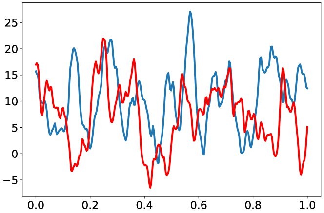
Figure 1: Two examples of random functions on the unit interval.

The problem setup is as follows. We sequentially perform 35 observations of a given function $f$. Each observation is either a point observation $f(x)$ ($w=0$), or an integral observation of width $w>0$:

$$\widetilde{f}_{w}(q):=\frac{1}{w}\int_{q-w/2}^{q+w/2}\text{d}x~{}f(x)\,,\quad 0\leq q\leq 1\,.$$

The two initial query points and their widths are chosen at random, and ensuing observations are coordinated according to Algorithm 1. There is a free parameter $0<\alpha<2$ for DC (Székely et al., 2007; Székely and Rizzo, 2013) and we use $\alpha\in\{0.5,1,1.5\}$ to check $\alpha$-dependence of the effectiveness of Algorithm 1. $\{\widehat{\mathbf{x}}_{n}\}_{n=1:N}$ are taken to be 120 equidistant points that uniformly cover $[0,1]$, $M=200$, and $\{w_{j}\}_{j=1:J}=\{0,0.0875,0.175,0.2625,0.35,0.4375,0.525,0.6125,0.7\}$. Every time the mean of $f$ is updated (line 5) we evaluate the quality of our prediction by measuring $R^{2}$, i.e., the coefficient of determination (higher is better). We have run Algorithm 1 for $64$ different random functions and took the average of $R^{2}$.

As baselines, we have also implemented two other policies for sequential querying. The first is a random policy that selects both the next query point and the next width completely randomly. The second is a zero-width max-variance policy, which avoids integral observations entirely and only performs point observations $(w=0)$ in such a way that the point that corresponds to the maximal predictive variance is selected as the next query point (as in line 10 of Algorithm 1). It makes no use of DC.

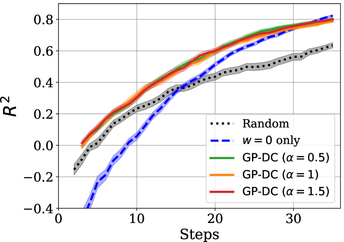
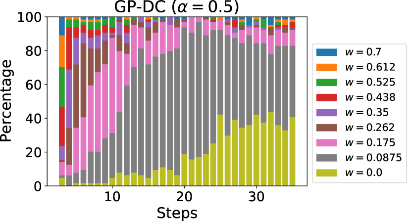
Figure 2: Performance of GP-DC and the two baseline methods as measured by coefficient of determination.

Figure 3: Widths of integral observations adaptively chosen by GP-DC for 64 random functions.

The result of numerical experiments is shown in Figure 3. $\alpha$-dependence of GP-DC appears to be very weak. GP-DC is not only significantly better than the random policy but also outperforms the $w=0$ policy up to 32 steps. In fact, the latter exhibits a very low score for the initial steps due to the fact that point observations fail to capture the global terrain of a function.

Figure 3 displays the distribution of the width of observations selected adaptively by GP-DC ($\alpha=0.5$) at each step. Interestingly, it favors relatively broad widths at the initial 10 steps, which is followed by an intermediate regime where the second smallest width $w=0.0875$ is dominant. Finally, a point observation gradually increases its proportion. This can be interpreted intuitively: broad observations is an efficient means to garner information on the global shape of the function, but it is soon exhausted and one has to resort to finer observations to acquire more local information. It is noteworthy that such adaptive decisions about the optimal resolution are made automatically by simply maximizing DC, with no subjective manual tuning of the policy.

The next question is whether GP-DC can handle derivative observations or not. However, care must be taken since a derivative observation is in general quite vulnerable to noises. To stabilize the optimization process, a Gaussian filter of width $w>0$ is applied before differentiation, i.e., a coarse-grained gradient defined by

$$\frac{\partial}{\partial q}f_{w}(q):=\frac{\partial}{\partial q}\int\text{d}x\;f(x)\frac{1}{\sqrt{2\pi w^{2}}}\mathrm{e}^{-(x-q)^{2}/(2w^{2})}$$

is considered. The problem setup is as follows. We first generate 48 random functions on the interval $[0,1]$. For each function $f$, $f(0)$ and $f(1)$ are observed first, and then 33 gradients are sequentially observed. The width is selected from $\{w_{j}\}_{j=1:J}=${0.02, 0.06, 0.12, 0.2, 0.3, 0.4, 0.5, 0.6, 0.7} according to GP-DC $(\alpha=1)$. The number of samples used for DC is $M=300$. For comparison, two other policies were also implemented: (i) a random policy that selects both the width and query point $q\in[0,1]$ at random and (ii) a narrow-gradient policy that exclusively adopts the smallest width $w=0.02$ and selects the point of maximal predictive variance sequentially.

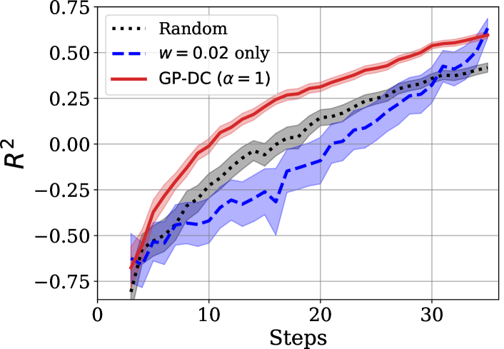
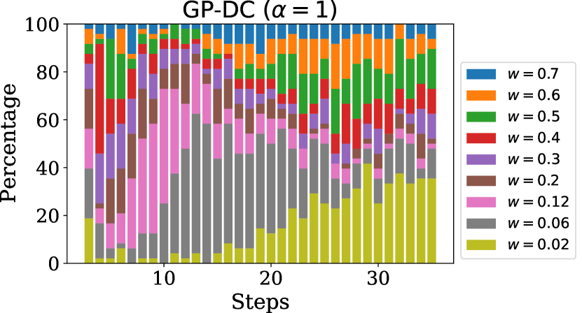
Figure 4: Performance of GP-DC and the two baseline methods for gradient observations.

Figure 5: Widths of gradient observations adaptively chosen by GP-DC for 48 random functions.

Figure 5 shows the result of numerical experiments. Clearly GP-DC shows superiority over the baselines. The $w=0.02$ policy catches up with GP-DC at the 35th step, but its variance remains large over all steps. In contrast, the variance of GP-DC is impressively small, indicating its stable performance for a variety of functions. In Figure 5 we display the statistics of widths that were actually selected by GP-DC at each step. One can see a monotonic increase of the proportion of $w=0.02$. On the contrary, $w=0.06$ is favored only during intermediate steps.

3.4 Test on real data

The proposed algorithm was tested on a surveillance task of the landscape of the Grand Canyon in the manner emulating remote sensing from airplane or satellite. The digital elevation model available from (USGS, ), shown in Figure 6, was used for the test. The size of the image is $2800\times 2800$ pixels, which was rescaled to a unit square $[0,1]^{2}$.

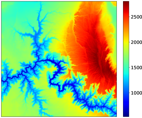
Figure 6: Digital elevation model of the Grand Canyon.

There are basically two approaches to implement integral observations in two dimensions: either use line integrals as in (Purisha et al., 2019; Longi et al., 2020), or use area integrals as in (Tanaka et al., 2019). The latter approach was adopted for the test. Specifically, it was assumed that the integral of elevation is observed over a disk of radius $r$ centered at $\mathbf{q}$,

$$f_{r}(\mathbf{q}):=\int_{|\mathbf{x}-\mathbf{q}|\leq r}\text{d}\mathbf{x}~{}f(\mathbf{x})$$

where $r\in\{0,0.05,0.1,0.15,0.2,0.25,0.3,0.35,0.4\}$. ($r=0$ is defined as the normal point observation.) When the integral domain overlaps outside of $[0,1]^{2}$, the function is extended by reflection about the edge. For an efficient numerical integration over a disk, we employed the quadrature formula in (Bojanov and Petrova, 1998, Theorem 1). Despite this, a 2d integral is numerically very expensive. The bottleneck is line 9 of Algorithm 1, where the variance needs to be computed for $N$ points simultaneously. It requires a computation of an $N\times N$ symmetric gram matrix whose elements are double 2d (i.e., 4d) integrals of the kernel function. Computation of these $\frac{1}{2}N^{2}$ integrals becomes quickly infeasible when $N$ is large ($>100$). To cope with this problem, we made an evenly spaced meshgrid of size $30\times 30$ over $[0,1]^{2}$ and from there selected 100 points randomly, for every $t$ and $j$ in Algorithm 1.

For comparison, two other policies were also implemented: (i) a random policy (selecting $\mathbf{q}$ and $r$ completely at random) and (ii) a policy that exclusively makes $r=0$ observations (i.e., a point with maximal predictive variance is sequentially observed). Each of the three algorithms was run 16 times with different random seeds. $M=300$ was used for GP-DC.

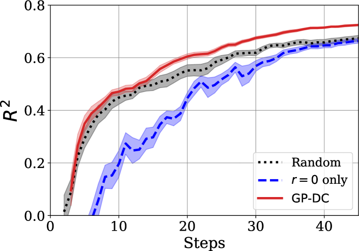
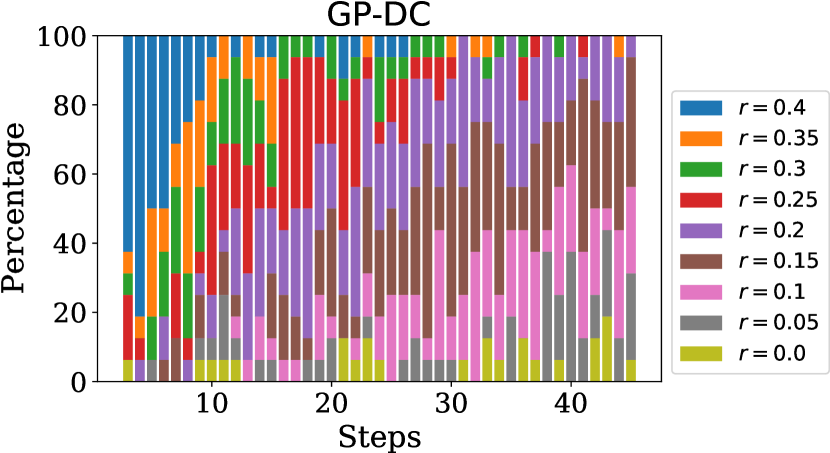
Figure 7: Performance of GP-DC and the two baseline methods for evaluating the Grand Canyon data.

Figure 8: Widths of integral observations adaptively chosen by GP-DC for 16 random initial conditions for evaluating the Grand Canyon data.

The results of the performance evaluation are presented in Figure 8. Clearly the policy with $r=0$ performs worst, indicating high efficiency of integral observations as a means of collecting distributed data. GP-DC is almost degenerate with the random policy up to 14th step, but from there on GP-DC consistently outperforms the random policy. The random policy needs 45 steps to attain $R^{2}\geq 0.68$. In contrast, GP-DC needs only 30 steps, implying more than $30\%$ reduction of required steps.

The distribution of $r$ selected by GP-DC at each step is shown in Figure 8. At the initial stages, $r\gtrsim 0.3$ is strongly favored, whereas at the later stages $r\lesssim 0.15$ is favored. This result implies that the proposed algorithm initially searches for long-wavelength information but later turns to shorter-wavelength information, which is in accord with that presented in Sec. 3.3.

4 GP-DC for black-box maximization

4.1 Algorithm

Hereafter we focus on the orthodox setup of BO, in which it is required to identify the maximum of a black-box function with the least number of observations. Unlike in Sec. 3, the following evaluations are limited to point observations for simplicity. Note that each observation of $f$ may be noisy. Our main proposition is Algorithm 2. The essential step is line 13, which identifies the next query point by maximizing DC with the surmised max-values of $f$.

Algorithm 2 GP-DC for maximum search

1:$\mathbf{x}_{0}\in\chi$: Initial query point
 - $\{\widehat{\mathbf{x}}_{n}\}_{n=1:N}\subset\chi$: Representative points of $\chi$
 - $M\in\mathbb{N}$: Number of samples to be drawn from
 -       posterior distribution of $f$

2:Observe $f$ at $\mathbf{x}_{0}$ and get $y_{0}$

3:$D_{0}\leftarrow\{(\mathbf{x}_{0},y_{0})\}$

4:for $t=1,2,\dots$ do

5:     Optimize hyperparameters of GP model
 - using on $D_{t-1}$

6:     Compute mean and covariance of $f$ over
 - $\{\widehat{\mathbf{x}}_{n}\}$ using on $D_{t-1}$

7:     Draw $M$ samples of $f$ over $\{\widehat{\mathbf{x}}_{n}\}$

8:     Maximize each sample and obtain the set of max
 - values $\{\mathrm{f}^{\max}_{m}\}_{m=1:M}\in\mathbb{R}^{M}$

9:     DC-list $\leftarrow\emptyset$

10:     for $n=1,2,\dots,N$ do

11:         For $M$ samples of $f$ in line 6, query the value
 -   at $\mathbf{x}=\widehat{\mathbf{x}}_{n}$ and obtain $\{\mathrm{f}_{m}^{(n)}\}_{m=1:M}\in\mathbb{R}^{M}$

12:         Compute DC between $\{\mathrm{f}^{\max}_{m}\}_{m=1:M}$ and
 -   $\{\mathrm{f}_{m}^{(n)}\}_{m=1:M}$

13:         Define DC-list$[n]:=$ DC$(\{\mathrm{f}^{\max}_{m}\},\{\mathrm{f}_{m}^{(n)}\})$      

14:     $\widetilde{n}\leftarrow\mathrm{arg\,max}_{n}$ DC-list

15:     Observe $f$ at $\mathbf{x}=\widehat{\mathbf{x}}_{\widetilde{n}}$ and get $y_{t}$

16:     $D_{t}\leftarrow D_{t-1}\cup\{(\widehat{\mathbf{x}}_{\widetilde{n}},y_{t})\}$

Based on Algorithm 2, the following five algorithms are proposed. ($\alpha=1$ for all DC computations.)

• GP-dCor and GP-dCov
  In line 11 of Algorithm 2, DC could be either distance correlation or distance covariance. These are separately called GP-dCor and GP-dCov, respectively.

• GP-MIS
  In line 11 of Algorithm 2, DC could be replaced with MI. To avoid confusion with GP-MI in (Contal et al., 2014), this algorithm is referred to as GP-MIS, where the last S indicates sampling from the posterior distribution of $f$. We used mutual_info_regression implemented in scikit-learn (Pedregosa et al., 2011). Note that, although GP-MIS is conceptually akin to MES, the computational procedure is different.

• GP-dCor-X and GP-dCov-X
  In line 7 of Algorithm 2, we could also collect arg max (rather than max) of each sample of $f$: $\{\mathbf{x}^{\max}_{m}\}_{m=1:M}\in\chi^{M}$. Line 12 should then be modified to DC-list$[n]:=$ DC$(\{\mathbf{x}^{\max}_{m}\},\{\mathrm{f}_{m}^{(n)}\})$. This approach is referred to as GP-dCor-X or GP-dCov-X, depending on whether distance correlation or distance covariance is used.

4.2 Test on random functions

The performances of the five proposed algorithms were numerically compared with those of eight baseline methods: Random, VarMax, PI, EI, GP-UCB, GP-MI, MES, and Brent. Here, VarMax is a purely exploratory policy that queries the point of maximal predictive variance. For PI we use Eq. (2) in (Brochu et al., 2010) with $\xi=10^{-3}$. As for GP-UCB (Srinivas et al., 2012), we use Eq. (5) in (Brochu et al., 2010) with $\nu=1$ and $\delta=0.05$. For GP-MI (Contal et al., 2014), we use $\alpha=\log(2/\delta)$ with $\delta=10^{-10}$. For MES we use Eq. (6) in (Wang and Jegelka, 2017) with $K=100$. Finally, for Brent (Brent, 1973), we use the ${\tt minimize{\verb|_|}scalar}$ function of scipy (Virtanen et al., 2020). The first two query points are chosen randomly for all methods except for Brent for which all points including the first ones are selected adaptively.

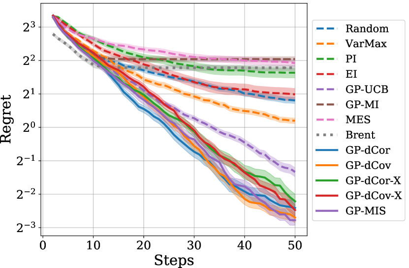
Figure 9: Performance of optimization algorithms evaluated on 256 random functions in one dimension. The five solid lines denote the proposed algorithms.

256 random functions on the interval $[0,1]$ were generated in the manner described in Sec. 3.3. For each function, 50 observations are made sequentially, and after every observation, the goodness of each algorithm was measured by so-called regret (lower is better) defined at step $T$ as

$$\text{Regret}_{T}:=\max_{\mathbf{x}}f(\mathbf{x})-\max_{1\leq t\leq T}y_{t}$$

where $y_{t}$ is the observed value of $f$ at step $t$. Average regret obtained from numerical simulations is plotted in Figure 9 on a log scale. It is clear that the proposed algorithms outperform all the baselines. Among the baselines, the best contender is GP-UCB, which seems to attain a good balance between exploration and exploitation. In contrast, methods such as GP-MI stop exploration way too early and get trapped in a local minimum. And note that GP-dCor, GP-dCov and GP-MIS are slightly better than GP-dCor-X and GP-dCov-X.

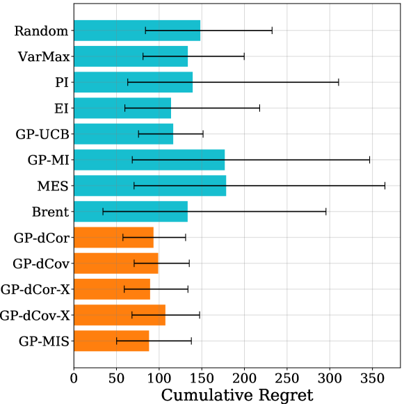
Figure 10: Cumulative regret of optimization algorithms evaluated on 256 random functions in one dimension (lower is better). The thick bars represent the median and the error bars denote 25 and 75 percentiles.

Accumulated regret $\sum_{T=2}^{50}\text{Regret}_{T}$ is plotted in Figure 10. All the baseline methods, except for GP-UCB, suffer a heavy tail towards high cumulative regret, implying that methods such as PI, GP-MI, and MES tend to fail completely for some functions. In contrast, the proposed methods have relatively short error bars, indicating their robustness.

4.3 Test on benchmark functions

Next we perform numerical tests on four popular benchmark functions in two dimensions: Himmelblau function, Eggholder function, Branin function and Goldstein-Price function. Details of these functions are described in Appendix. For each function, 50 observations are sequentially made, where the first two query points were chosen randomly. We have run each algorithm 64 times with different random initial points. Average of regret at each step is plotted in Figure 11, and cumulative regret $\sum_{T=20}^{50}\text{Regret}_{T}$ is listed in Table 1. (Regrets for the first 19 steps are omitted to better characterize behaviors at the later stages of optimization.) In Table 1, the normalization is such that median cumulative regret of the random policy is equal to 1.

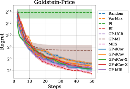
Figure 11: Regret obtained by algorithms averaged over 64 random initial conditions for four standard benchmark functions.

Table 1: Median of cumulative regret $\sum_{T=20}^{50}\text{Regret}_{T}$ for 64 random initial conditions, normalized in units of the random policy’s score. $25\%$ and $75\%$ percentiles are also shown. The last column is the average for the four functions.

	Himmelblau	Eggholder	Branin	$\begin{subarray}{c}\text{Goldstein-}\\ \text{Price}\end{subarray}$	Avg.
Random	1.00${}^{+0.64}_{-0.56}$	1.00${}^{+0.21}_{-0.34}$	1.00${}^{+0.35}_{-0.80}$	1.00${}^{+0.33}_{-0.48}$	1.00 ​
VarMax	1.08${}^{+0.63}_{-0.34}$	0.89${}^{+0.15}_{-0.26}$	1.14${}^{+0.19}_{-0.45}$	0.96${}^{+0.68}_{-0.46}$	1.02
PI	0.00${}^{+0.09}_{-0.00}$	0.64${}^{+0.33}_{-0.36}$	9.82${}^{+10.74}_{-4.80}$	29.6${}^{+123.7}_{-12.2}$	10.0
EI	11.56${}^{+8.78}_{-5.42}$	2.12${}^{+0.52}_{-1.03}$	0.02${}^{+0.02}_{-0.01}$	0.27${}^{+0.25}_{-0.07}$	3.49
GP-UCB	0.52${}^{+0.22}_{-0.25}$	0.87${}^{+0.16}_{-0.35}$	0.51${}^{+0.15}_{-0.32}$	0.59${}^{+0.47}_{-0.22}$	0.62
GP-MI	0.39${}^{+1.00}_{-0.30}$	1.45${}^{+0.23}_{-0.57}$	0.70${}^{+0.29}_{-0.66}$	0.39${}^{+0.23}_{-0.17}$	0.73
MES	11.88${}^{+4.50}_{-5.40}$	2.65${}^{+0.39}_{-0.70}$	0.07${}^{+0.38}_{-0.06}$	0.41${}^{+0.15}_{-0.14}$	3.75
GP-dCor	0.45${}^{+0.18}_{-0.27}$	0.98${}^{+0.28}_{-0.24}$	0.07${}^{+0.12}_{-0.05}$	0.44${}^{+0.32}_{-0.16}$	0.49 ​
GP-dCov	0.54${}^{+0.21}_{-0.31}$	0.87${}^{+0.30}_{-0.26}$	0.32${}^{+0.30}_{-0.19}$	0.62${}^{+0.47}_{-0.24}$	0.59
GP-dCor-X	0.24${}^{+0.11}_{-0.11}$	0.76${}^{+0.21}_{-0.23}$	0.05${}^{+0.07}_{-0.03}$	0.51${}^{+0.39}_{-0.24}$	0.39
GP-dCov-X	0.46${}^{+0.19}_{-0.19}$	0.77${}^{+0.31}_{-0.32}$	0.32${}^{+0.15}_{-0.19}$	0.54${}^{+0.52}_{-0.26}$	0.52
GP-MIS	0.28${}^{+0.20}_{-0.13}$	0.86${}^{+0.20}_{-0.33}$	0.04${}^{+0.13}_{-0.03}$	0.52${}^{+0.33}_{-0.25}$	0.43

The results described above show that PI and EI exhibit a complementary behavior: PI performs the best for Himmelblau and Eggholder, while EI performs the best for Branin and Goldstein-Price, and yet their regrets are quite high for the other two functions, implying their serious lack of robustness. MES has the same downside. Among the baselines, GP-UCB is the only one that is superior to the random policy for all the four tasks. It is noteworthy that the five proposed algorithms on average outperform all the baselines, including GP-UCB. In particular, GP-dCor-X has the lowest regret of $0.39$. The second best is GP-MIS with regret of $0.43$. It is thus concluded that GP-DC is a robust and effective method of optimizing a black-box function with improved performance compared to state-of-the-art methods.

5 Conclusion and outlook

In this paper, a novel Bayesian optimization approach called GP-DC was proposed and evaluated. This approach computes distance correlation and distance covariance to determine the next evaluation point. It is easy to implement, obviates the need for laborious hyperparameter tuning, and performs as well as or even better than state-of-the-art methods such as GP-UCB and MES across a variety of maximization tasks. We have also demonstrated the power of GP-DC for Bayesian experimental design, where the goal is not to determine the maximum of a function but to globally probe the function as accurately as possible with least observations. There GP-DC enables to execute efficient sequential integral observations with adaptive integration width. Our work has potential applications in such fields as computed tomography, remote sensing with satellites, materials experiments, and hyperparameter tuning of machine-learning models, where a measurement is either costly, time-consuming or invasive. The proposed approach also provides a principled means to optimize sequential acquisition of spatially or temporarily aggregated data that often arises in sociology and economics. One of possible future directions of research is to extend the current work to a batch setup where multiple evaluations are performed in parallel.

Appendix

The benchmark functions used in Sec. 4.3 are defined in the following. The definitions conform to the conventions of https://www.sfu.ca/~ssurjano/index.html and https://en.wikipedia.org/wiki/Test_functions_for_optimization to which the reader is referred for further details. All the functions below are usually minimized by optimization algorithms. In Sec. 4.3 the negative of the functions is taken, and maximization problems are considered.

1. Himmelblau function

   $$f(x_{1},x_{2})=(x_{1}^{2}+x_{2}-11)^{2}+(x_{1}+x_{2}^{2}-7)^{2}.$$

   The domain is $-6\leq x_{1}\leq 6$ and $-6\leq x_{2}\leq 6$. The minimum value is $0$.

2. Eggholder function

   $$\begin{array}[]{rl}f(x_{1},x_{2})=\!\!\!\!&-(x_{2}+47)\sin\left(\sqrt{\left|x_{2}+\frac{x_{1}}{2}+47\right|}\right)\\ &-x_{1}\sin\left(\sqrt{|x_{1}-(x_{2}+47)|}\right).\end{array}$$

   The domain is $-512\leq x_{1}\leq 512$ and $-512\leq x_{2}\leq 512$. The minimum value is $-959.640663$.

3. Branin (or Branin-Hoo) function

   $$f(x_{1},x_{2})=a(x_{2}-bx_{1}^{2}+cx_{1}-r)^{2}+s(1-t)\cos x_{1}+s$$

   where $a=1$, $b=5.1/(4\pi^{2})$, $c=5/\pi$, $r=6$, $s=10$ and $t=1/(8\pi)$. The domain is $-5\leq x_{1}\leq 10$ and $0\leq x_{2}\leq 15$. The minimum value is $0.39788736$.

4. Goldstein-Price function

   $$f(x_{1},x_{2}) =\left[1+(x_{1}+x_{2}+1)^{2}U\right]$$

   $$\quad\times\left[30+(2x_{1}-3x_{2})^{2}V\right]$$

   where

   $$U =19-14x_{1}+3x_{1}^{2}-14x_{2}+6x_{1}x_{2}+3x_{2}^{2}\,,$$

   $$V =18-32x_{1}+12x_{1}^{2}+48x_{2}-36x_{1}x_{2}+27x_{2}^{2}\,.$$

   The domain is $-2\leq x_{1}\leq 2$ and $-2\leq x_{2}\leq 2$. The minimum value is $3$.

References

- Adelsberg and Schwantes (2018) M. Adelsberg and C. Schwantes. Binned Kernels for Anomaly Detection in Multi-timescale Data using Gaussian Processes. In Proceedings of the KDD 2017: Workshop on Anomaly Detection in Finance, volume 71 of PMLR, pages 102–113, 2018.
- Ahmed et al. (2016) M. Ahmed, B. Shahriari, and M. Schmidt. Do we need “harmless” Bayesian optimization and “first-order” Bayesian optimization? BayesOpt, 2016.
- Ayush et al. (2020) K. Ayush, B. Uzkent, M. Burke, D. Lobell, and S. Ermon. Efficient Poverty Mapping using Deep Reinforcement Learning. 2020. arXiv:2006.04224.
- Bojanov and Petrova (1998) B. Bojanov and G. Petrova. Numerical integration over a disc. A new Gaussian quadrature formula. Numer. Math., 80:39–59, 1998.
- Brent (1973) R. P. Brent. Chapter 4: An Algorithm with Guaranteed Convergence for Finding a Zero of a Function. In Algorithms for Minimization without Derivatives. Prentice-Hall, 1973.
- Brochu et al. (2010) E. Brochu, V. M. Cora, and N. de Freitas. A Tutorial on Bayesian Optimization of Expensive Cost Functions, with Application to Active User Modeling and Hierarchical Reinforcement Learning. 2010. arXiv:1012.2599.
- Burger et al. (2020) M. Burger, A. Hauptmann, T. Helin, N. Hyvönen, and J. Puska. Sequentially optimized projections in X-ray imaging, 2020. arXiv:2006.12579.
- Carreño (2020) C. R. Carreño. dcor. 2020. URL https://github.com/vnmabus/dcor.
- Chen et al. (2015) Y. Chen, S. H. Hassani, A. Karbasi, and A. Krause. Sequential Information Maximization: When is Greedy Near-optimal? In Proceedings of The 28th Conference on Learning Theory, volume 40 of PMLR, pages 338–363, 2015.
- Contal et al. (2014) E. Contal, V. Perchet, and N. Vayatis. Gaussian Process Optimization with Mutual Information. In Proceedings of the 31st International Conference on Machine Learning, volume 32 of PMLR, pages 253–261. PMLR, 2014.
- Cover and Thomas (2012) T. M. Cover and J. A. Thomas. Elements of Information Theory. Wiley, 2nd edition, 2012.
- Eriksson et al. (2018) D. Eriksson, K. Dong, E. Lee, D. Bindel, and A. G. Wilson. Scaling Gaussian Process Regression with Derivatives. In Advances in Neural Information Processing Systems 31, pages 6867–6877. 2018.
- Forrester et al. (2007) A. I. J. Forrester, A. Sóbester, and A. J. Keane. Multi-fidelity optimization via surrogate modelling. Proc. R. Soc. A., 463:3251–3269, 2007.
- François-Lavet et al. (2018) V. François-Lavet, P. Henderson, R. Islam, M. G. Bellemare, and J. Pineau. An Introduction to Deep Reinforcement Learning. Foundations and Trends in Machine Learning, 11:219–354, 2018.
- Frazier (2018) P. I. Frazier. A Tutorial on Bayesian Optimization. 2018. arXiv:1807.02811.
- Golovin and Krause (2011) D. Golovin and A. Krause. Adaptive Submodularity: Theory and Applications in Active Learning and Stochastic Optimization. Journal of Artificial Intelligence Research, 42:427–486, 2011.
- Hamelijnck et al. (2019) O. Hamelijnck, T. Damoulas, K. Wang, and M. Girolami. Multi-resolution Multi-task Gaussian Processes. In Advances in Neural Information Processing Systems, volume 32, pages 14025–14035, 2019.
- Hendriks et al. (2018) J. N. Hendriks, C. Jidling, A. Wills, and T. B. Schön. Evaluating the squared-exponential covariance function in Gaussian processes with integral observations, 2018. arXiv:1812.07319.
- Hennig and Schuler (2012) P. Hennig and C. J. Schuler. Entropy Search for Information-Efficient Global Optimization. Journal of Machine Learning Research, 13:1809–1837, 2012.
- Hernández-Lobato et al. (2014) J. M. Hernández-Lobato, M. W. Hoffman, and Z. Ghahramani. Predictive Entropy Search for Efficient Global Optimization of Black-box Functions. In Advances in Neural Information Processing Systems, volume 27, pages 918–926, 2014.
- Hoffman and Ghahramani (2015) M. W. Hoffman and Z. Ghahramani. Output-space predictive entropy search for flexible global optimization. NIPS workshop on Bayesian Optimization, 2015.
- Jidling et al. (2019) C. Jidling, J. Hendriks, T. B. Schön, and A. Wills. Deep kernel learning for integral measurements, 2019. arXiv:1909.01844.
- Jones et al. (1998) D. R. Jones, M. Schonlau, and W. J. Welch. Efficient global optimization of expensive black-box functions. Journal of Global Optimization, 13:455–492, 1998.
- Kanazawa et al. (2020) T. Kanazawa, A. Asahara, and H. Morita. Accelerating small-angle scattering experiments with simulation-based machine learning. Journal of Physics: Materials, 3:015001, 2020.
- Kushner (1964) H. J. Kushner. A New Method of Locating the Maximum Point of an Arbitrary Multipeak Curve in the Presence of Noise. Journal of Basic Engineering, 86:97–106, 1964.
- Law et al. (2018) H. C. L. Law, D. Sejdinovic, E. Cameron, T. C. D. Lucas, S. Flaxman, K. Battle, and K. Fukumizu. Variational learning on aggregate outputs with Gaussian processes. In Proceedings of the 32nd International Conference on Neural Information Processing Systems, pages 6084–6094, 2018.
- Lázaro-Gredilla et al. (2010) M. Lázaro-Gredilla, J. Quiñnero-Candela, C. E. Rasmussen, and A. R. Figueiras-Vidal. Sparse Spectrum Gaussian Process Regression. Journal of Machine Learning Research, 11:1865–1881, 2010.
- Li (2017) Y. Li. Deep Reinforcement Learning: An Overview, 2017. arXiv:1701.07274.
- Longi et al. (2020) K. Longi, C. Rajani, T. Sillanpää, J. Mäkinen, T. Rauhala, A. Salmi, E. Haeggström, and A. Klami. Sensor Placement for Spatial Gaussian Processes with Integral Observations. In Proceedings of the 36th Conference on Uncertainty in Artificial Intelligence (UAI), volume 124 of PMLR, pages 1009–1018, 2020.
- Moss et al. (2020) H. B. Moss, D. S. Leslie, and P. Rayson. MUMBO: MUlti-task Max-value Bayesian Optimization, 2020. arXiv:2006.12093.
- Osborne et al. (2009) M. A. Osborne, R. Garnett, and S. J. Roberts. Gaussian processes for global optimization. In 3rd International Conference on Learning and Intelligent Optimization (LION3), 2009.
- Pedregosa et al. (2011) F. Pedregosa, G. Varoquaux, A. Gramfort, V. Michel, B. Thirion, O. Grisel, M. Blondel, P. Prettenhofer, R. Weiss, V. Dubourg, J. Vanderplas, A. Passos, D. Cournapeau, M. Brucher, M. Perrot, and E. Duchesnay. Scikit-learn: Machine Learning in Python. Journal of Machine Learning Research, 12:2825–2830, 2011.
- Purisha et al. (2019) Z. Purisha, C. Jidling, N. Wahlström, T. B. Schön, and S. Särkkä. Probabilistic approach to limited-data computed tomography reconstruction. Inverse Problems, 35(10):105004, 2019.
- Rasmussen and Williams (2006) C. E. Rasmussen and C. K. I. Williams. Gaussian Processes for Machine Learning. MIT Press, 2006.
- Shahriari et al. (2016) B. Shahriari, K. Swersky, Z. Wang, R. P. Adams, and N. de Freitas. Taking the Human Out of the Loop: A Review of Bayesian Optimization. Proceedings of the IEEE, 104(1):148–175, 2016.
- Smith et al. (2018) M. T. Smith, M. A. Alvarez, and N. D. Lawrence. Gaussian Process Regression for Binned Data, 2018. arXiv:1809.02010.
- Snoek et al. (2012) J. Snoek, H. Larochelle, and R. P. Adams. Practical Bayesian Optimization of Machine Learning Algorithms. In Advances in Neural Information Processing Systems, volume 25, pages 2951–2959, 2012.
- Solak et al. (2002) E. Solak, R. Murray-Smith, W. E. Leithead, D. J. Leith, and C. E. Rasmussen. Derivative Observations in Gaussian Process Models of Dynamic Systems. In Proceedings of the 15th International Conference on Neural Information Processing Systems, pages 1057–1064. MIT Press, 2002.
- Srinivas et al. (2012) N. Srinivas, A. Krause, S. M. Kakade, and M. W. Seeger. Information-Theoretic Regret Bounds for Gaussian Process Optimization in the Bandit Setting. IEEE Transactions on Information Theory, 58:3250–3265, 2012.
- Székely and Rizzo (2013) G. J. Székely and M. L. Rizzo. Energy statistics: A class of statistics based on distances. Journal of Statistical Planning and Inference, 143(8):1249–1272, 2013.
- Székely et al. (2007) G. J. Székely, M. L. Rizzo, and N. K. Bakirov. Measuring and Testing Dependence by Correlation of Distances. Annals of Statistics, 35(6):2769–2794, 2007.
- Takeno et al. (2020) S. Takeno, H. Fukuoka, Y. Tsukada, T. Koyama, M. Shiga, I. Takeuchi, and M. Karasuyama. Multi-fidelity Bayesian Optimization with Max-value Entropy Search and its Parallelization. In Proceedings of the 37th International Conference on Machine Learning, volume 119 of PMLR, pages 9334–9345, 2020.
- Tanaka et al. (2019) Y. Tanaka, T. Tanaka, T. Iwata, T. Kurashima, M. Okawa, Y. Akagi, and H. Toda. Spatially Aggregated Gaussian Processes with Multivariate Areal Outputs. In Advances in Neural Information Processing Systems, volume 32, pages 3005–3015, 2019.
- Tanskanen et al. (2020) V. Tanskanen, K. Longi, and A. Klami. Non-Linearities in Gaussian Processes with Integral Observations. In 2020 IEEE 30th International Workshop on Machine Learning for Signal Processing (MLSP), pages 1–6, 2020.
- (45) USGS. URL https://pubs.usgs.gov/ds/121/grand/grand.html.
- Uzkent and Ermon (2020) B. Uzkent and S. Ermon. Learning When and Where to Zoom with Deep Reinforcement Learning. 2020.
- Villemonteix et al. (2009) J. Villemonteix, E. Vazquez, and E. Walter. An informational approach to the global optimization of expensive-to-evaluate functions. Journal of Global Optimization, 44:509, 2009.
- Virtanen et al. (2020) P. Virtanen et al. SciPy 1.0: Fundamental Algorithms for Scientific Computing in Python. Nature Methods, 17:261–272, 2020.
- Wang and Jegelka (2017) Z. Wang and S. Jegelka. Max-Value Entropy Search for Efficient Bayesian Optimization. In Proceedings of the 34th International Conference on Machine Learning, volume 70, pages 3627–3635, 2017.
- Wu et al. (2017a) A. Wu, M. C. Aoi, and J. W. Pillow. Exploiting gradients and Hessians in Bayesian optimization and Bayesian quadrature, 2017a. arXiv:1704.00060.
- Wu et al. (2017b) J. Wu, M. Poloczek, A. G. Wilson, and P. Frazier. Bayesian Optimization with Gradients. In Advances in Neural Information Processing Systems, volume 30, pages 5267–5278, 2017b.
- Yousefi et al. (2019) F. Yousefi, M. T. Smith, and M. Álvarez. Multi-task Learning for Aggregated Data using Gaussian Processes. In Advances in Neural Information Processing Systems, volume 32, pages 15076–15086, 2019.