Gravitational wave cosmology I: high frequency approximation

Abstract

In this paper, we systematically study gravitational waves (GWs) first produced by remote compact astrophysical sources and then propagating in our inhomogeneous universe through cosmic distances, before arriving at detectors. To describe such GWs properly, we introduce three scales, $\lambda,\;L_{c}$ and $L$, denoting, respectively, the typical wavelength of GWs, the scale of the cosmological perturbations, and the size of the observable universe. For GWs to be detected by the current and foreseeable detectors, the condition $\lambda\ll L_{c}\ll L$ holds. Then, such GWs can be approximated as high-frequency GWs and be well separated from the background $\gamma_{\mu\nu}$ by averaging the spacetime curvatures over a scale $\ell$, where $\lambda\ll\ell\ll L_{c}$, and $g_{\mu\nu}=\gamma_{\mu\nu}+\epsilon h_{\mu\nu}$ with $h_{\mu\nu}$ denoting the GWs. In order for the backreaction of the GWs to the background spacetimes to be negligible, we must assume that $\left|h_{\mu\nu}\right|\ll 1$, in addition to the condition $\epsilon\ll 1$, which are also the conditions for the linearized Einstein field equations for $h_{\mu\nu}$ to be valid. Such studies can be significantly simplified by properly choosing gauges, such as the spatial, traceless, and Lorenz gauges. We show that these three different gauge conditions can be imposed simultaneously, even when the background is not vacuum, as long as the high-frequency GW approximation is valid. However, to develop the formulas that can be applicable to as many cases as possible, in this paper we first write down explicitly the linearized Einstein field equations by imposing only the spatial gauge. Then, applying these formulas together with the geometrical optics approximation to such GWs, we find that they still move along null geodesics and its polarization bi-vector is parallel-transported, even when both the cosmological scalar and tensor perturbations are present. In addition, we also calculate the gravitational integrated Sachs-Wolfe effects due to these two kinds of perturbations, whereby the dependences of the amplitude, phase and luminosity distance of the GWs on these perturbations are read out explicitly.

I Introduction

The detection of the first gravitational wave (GW) from the coalescence of two massive black holes (BHs) by the advanced Laser Interferometer Gravitational-Wave Observatory (aLIGO) marked the beginning of a new era, the GW astronomy Ref1 . Following this observation, soon more than 50 GWs were detected by the LIGO/Virgo scientific collaboration GWTC1 ; GWTC2 ; aLIGO . The outbreak of interest on GWs and BHs has further gained momenta after the detection of the shadow of the M87 BH EHTa ; EHTb ; EHTc ; EHTd ; EHTe ; EHTf .

One of the remarkable observational results is the discovery that the mass of an individual BH in these binary systems can be much larger than what was previously expected, both theoretically and observationally Ref4 ; Ref5 ; Ref6 , leading to the proposal and refinement of various formation scenarios, see, for example, Ref7 ; Ref8 ; SSTY18 ; LIGO-Virgo20 , and references therein. A consequence of this discovery is that the early inspiral phase may also be detectable by space-based observatories, such as LISA PAS17 , TianQin TianQin , Taiji Taiji , and DECIGO DECIGO , for several years prior to their coalescence AS16 ; Moore15 . Multiple observations with different detectors at different frequencies of signals from the same source can provide excellent opportunities to study the evolution of the binary in detail. Since different detectors observe at disjoint frequency bands, together they cover different evolutionary stages of the same binary system. Each stage of the evolution carries information about different physical aspects of the source. As a result, multi-band GW detections will provide an unprecedented opportunity to test different theories of gravity in the strong field regime Carson:2019kkh .

Recently, some of the present authors generalized the post-Newtonian (PN) formalism to certain modified theories of gravity and applied it to the quasi-circular inspiral of compact binaries. In particular, we calculated in detail the waveforms, GW polarizations, response functions and energy losses due to gravitational radiation in Brans-Dicke (BD) theory Ref23 , screened modified gravity (SMG) Tan18 ; Ref25 ; Ref25b , and gravitational theories with parity violations QZZW19 ; ZZQW20 ; ZLWZWWZ20 ; QZZW20 to the leading PN order, with which we then considered projected constraints from the third-generation detectors. Such studies have been further generalized to triple systems Kai19 ; Zhao19 in Einstein-aether ($\ae$-) theory JM04 ; Jacobson08 ; OMW18 . When applying such formulas to the first relativistic triple system discovered in 2014 Ransom14 , we studied the radiation power, and found that quadrupole emission has almost the same amplitude as that in general relativity (GR), but the dipole emission can be as large as the quadrupole emission. This can provide a promising window to place severe constraints on $\ae$-theory with multi-band GW observations Ref17 ; Carson:2019yxq .

More recently, we revisited the problem of a binary system of non-spinning bodies in a quasi-circular inspiral within the framework of $\ae$-theory Foster06 ; Foster07 ; Yagi13 ; Yagi14 ; HYY15 ; GHLP18 , and provided the explicit expressions for the time-domain and frequency-domain waveforms, GW polarizations, and response functions for both ground- and space-based detectors in the PN approximation Zhang20 . In particular, we found that, when going beyond the leading order in the PN approximation, the non-Einsteinian polarization modes contain terms that depend on both the first and second harmonics of the orbital phase. With this in mind, we calculated analytically the corresponding parameterized post-Einsteinian parameters, generalizing the existing framework to allow for different propagation speeds among scalar, vector and tensor modes, without assuming the magnitude of its coupling parameters, and meanwhile allowing the binary system to have relative motions with respect to the aether field. Such results will particularly allow for the easy construction of Einstein-aether templates that could be used in Bayesian tests of GR in the future.

It is remarkable to note that the space-based detectors mentioned above, together with the current and forthcoming ground-based ones, such as KAGRA KAGRA , Voyager Voyager , the Einstein Telescope (ET) ET and Cosmic Explorer (CE) CE , are able to detect GWs emitted from such systems as far as the redshift is about $z\simeq 100$ HE19 , which will result in a variety of profound scientific consequences. In particular, GWs propagating over such long cosmic distances will carry valuable information not only about their sources, but also about the detail of the cosmological expansion and inhomogeneities of the universe, whereby a completely new window to explore the universe by using GWs is opened, as so far our understanding of the universe almost all comes from observations of electromagnetic waves only (possibly with the important exceptions of cosmic rays and neutrinos) LL09 .

In this paper, we shall generalize our above studies to the cases in which the GWs are first generated by remote astrophysical sources and then propagate in the inhomogeneous universe through cosmic distances before arriving at detectors, either space- and/or ground-based ones. It should be noted that recently such studies have already attracted lots of attention, see, for example, Belgacem19 and references therein. In particular, using Isaacson’s high frequency GW formulas Isaacson68a ; Isaacson68b , Laguna et al studied the gravitational analogue of the electromagnetic integrated Sachs-Wolf (iSW) effects in cosmology, and found that the phase, frequency, and amplitude of the GWs experience iSW effects, in addition to the magnifications on the amplitude from gravitational lensing LLSY10 . More recently, Bertacca et al connected the results of Laguna et al obtained in real space frame to the observed frame, by using the cosmic rulers formulas SJ12 , whereby the corrections to the luminosity distance due to velocity, volume, lensing and gravitational potential effects were calculated BRBM17 .

On the other hand, Bonvin et al BCST17 studied the effects of the universe on the gravitational waveform, and found that the acceleration of the Universe and the peculiar acceleration of the binary with respect to the observer distort the gravitational chirp signals from the simplest GR prediction, not only a mere time independent rescaling of the chirp mass, but also the intrinsic parameter estimations for binaries visible by LISA. In particular, the effect due to the peculiar acceleration can be much larger than the one due to the Universe acceleration. Moreover, peculiar accelerations can introduce a bias in the estimation of parameters such as the time of coalescence and the individual masses of the binary. An error in the estimation of the time of coalescence made by LISA will have an impact on the prediction of the time at which the signal will be visible by ground based interferometers, for signals spanning both frequency bands.

Moreover, the correlations of such GWs with lensing fields from the cosmic microwave background and galaxies were studied MWS20 , whereby a new window to explore our universe by gravitational weak lensing was proposed.

Lately, GWs propagating in the curved universe has been further generalized to scalar-tensor theories Garoffolo19 , including Horndeski DFL20a ; DFL20b ; EZ20 and SMG EZ20 theories.

However, it should be noted that in all these studies, the cosmological tensor perturbations have been neglected (Except DFL20a ; DFL20b , in which the background is arbitrary.). As observing the primordial GWs (the tensor perturbations) is one of the main goals in the current and forthcoming cosmological observations CMB-S4 , in this paper we shall consider the cosmological background that consists of both the scalar and tensor perturbations, but restrict ourselves only to Einstein’s theory, and leave the generalizations to other theories of gravity to other occasions. What we are planning to do in the current paper are the following:

• First, to describe the GWs propagating through the inhomogeneous universe from cosmic distances to observers properly, we first introduce three scales, $\lambda,\;L_{c}$ and $L$, which denote, respectively, the typical wavelength of GWs, the scale of the cosmological perturbations, and the size of the observable universe. For GWs to be detected by the current and foreseeable detectors, we find that the condition

  $$\lambda\ll L_{c}\ll L,$$ (1.1)

  always holds. Then, such GWs can be approximated as high-frequency GWs , and be well separated from the background $\gamma_{\mu\nu}$ by averaging the spacetime curvatures over a scale $\ell$, where $\lambda\ll\ell\ll L_{c}$, and the total metric of the spacetime is given by

  $$g_{\mu\nu} = \gamma_{\mu\nu}+\epsilon h_{\mu\nu},$$ (1.2)

  where $\epsilon\simeq{\cal{O}}(\lambda/L)$, and $\gamma_{\mu\nu}$ denotes the background, while $h_{\mu\nu}$ represents the GWs. In order for the backreaction of the GWs to the background spacetimes to be negligible, we must assume that

  $$\left|h_{\mu\nu}\right|\ll 1,$$ (1.3)

  in addition to the condition $\epsilon\ll 1$, which are also the conditions for the linearized Einstein field equations for $h_{\mu\nu}$ to be valid.

• Such studies can be significantly simplified by properly imposing gauge conditions, such as the spatial, traceless, and Lorenz gauges, given, respectively, by

  $$\chi_{0\mu} = 0,$$ (1.4)

  $$\chi = 0,$$ (1.5)

  $$\nabla^{\nu}\chi_{\mu\nu} = 0,$$ (1.6)

  where

  $$\chi_{\mu\nu}\equiv h_{\mu\nu}-\frac{1}{2}\gamma_{\mu\nu}h,\quad h\equiv\gamma^{\mu\nu}h_{\mu\nu},$$ (1.7)

  and $\nabla^{\nu}$ denotes the covariant derivative with respect to $\gamma_{\mu\nu}$. We show that these three different gauge conditions can be imposed simultaneously, even when the background is not vacuum, as longer as the high-frequency GW approximations are valid.

• However, to develop the formulas that can be applicable to as many cases as possible, in this paper we write down explicitly the linearized Einstein field equations for $\chi_{\mu\nu}$ by imposing only the spatial gauge. Applying these formulas together with the geometrical optic approximations to such GWs, we find the well-known results MTW73 : they still move along null geodesics and its polarization bi-vector is parallel-transported, even when both the cosmological scalar and tensor perturbations are present. In addition, we also calculate the gravitational integrated Sachs-Wolfe (iSW) effects due to these two kinds of perturbations, whereby the dependences of the amplitude, phase and luminosity distance of the GWs on these perturbations are read off explicitly.

The rest of the paper is organized as follows: In Sec. II, after introducing the three different scales, $\lambda,L_{c},L$, we show that, for the GWs to be detected by the current and foreseeable both ground- and space-based detectors, such GWs can be well approximated as high frequency GWs. Then, we derive the Einstein field equations, and find that, to make the backreaction of the GWs to the background negligible, as well as to have the linearized Einstein field equations for $h_{\mu\nu}$ to be valid, the condition (1.3) must hold. In this section, we also provide a very brief review on the cosmological background that consists of both the cosmological and tensor perturbations. In Sec. III, we consider the gauge freedom for GWs, and show that the three different gauge conditions, (1.4)-(1.6), can be still imposed simultaneously, even when the background spacetime is not vacuum, as long as the high-frequency approximations are valid. Then, by imposing only the spatial gauge condition (1.4), we write down the linearized Einstein field equations for the GWs, so the formulas can be applied to cases with different choices of gauges. In Sec. IV we study the GWs with the geometrical optics approximation, and calculate the effects of the cosmological scalar and tensor perturbations on the amplitudes and phases of such GWs, and find the explicit expressions of the iSW effects due to both the cosmological scalar and tensor perturbations. When applying them to a binary system, we calculate explicitly the effects of these two kinds of the cosmological perturbations on the luminosity distance and the chirp mass [cf. Eq.(4.51)]. Finally, we summarize our main results in Sec. V, and present some concluding remarks.

There are also three appendices, A, B and C, in which some mathematical computations are presented. In particular, in Appendix A, we give a very brief review over the inhomogeneous universe, when both the cosmological scalar and tensor perturbations are present, while in Appendix B, we present the field equations for the GWs $\chi_{\mu\nu}$ by imposing only the spatial gauge (1.4). In Appendix C, we first decompose $\chi_{\mu\nu}$ as $\chi_{\mu\nu}=\chi_{\mu\nu}^{(0)}+\epsilon_{c}\chi_{\mu\nu}^{(1)}$ and then write down explicitly the field equations for $\chi_{\mu\nu}^{(1)}$ only with the spatial gauge.

Before proceeding to the next section, we would like to note that GWs produced by remote astrophysical sources and then propagating through the homogeneous and isotropic universe have been systematical studied by Ashtekar and his collaborators through a series of papers AshtekarI ; AshtekarII ; AshtekarIII ; AshtekarIIIa ; AshtekarIV ; Ashtekar20a ; Ashtekar20b , and various subtle issues related to the de Sitter background were clarified Ashtekar17a ; Ashtekar17b ; Ashtekar17c (See also Chu15 ; Bishop16 ; TW16 ; DH16 ; BGY17a ; BGY17b ; Chu17 ; HFZ19 ; FSW20 ).

In addition, in this paper we shall adopt the following conventions, which are different from those adopted in Isaacson68a ; Isaacson68b , but the same as those used in MM16 . In particular, in this paper the signature of the metric is ($-,+,+,+$), while the Christoffel symbols, Riemann and Ricci tensors, as well as the Ricci scalar, are defined, respectively, by

$$\Gamma^{\alpha}_{\mu\nu}\equiv\frac{1}{2}g^{\alpha\beta}\left(g_{\beta\nu,\mu}+g_{\beta\mu,\nu}-g_{\mu\nu,\beta}\right),$$ (1.8)

$$\left(D_{\alpha}D_{\beta}-D_{\beta}D_{\alpha}\right)X^{\mu}={R^{\mu}}_{\nu\alpha\beta}X^{\nu},$$

$$R_{\mu\nu}\equiv R^{\alpha}_{\;\;\mu\alpha\nu},\quad R\equiv g^{\mu\nu}R_{\mu\nu},$$

where $D_{\alpha}$ denotes the covariant derivative with respect to metric $g_{\mu\nu}$, $g_{\mu\nu,\lambda}\equiv\partial g_{\mu\nu}/\partial x^{\lambda}$, and

$$R^{\alpha}_{\;\;\mu\nu\lambda} = \Gamma^{\alpha}_{\mu\lambda,\nu}-\Gamma^{\alpha}_{\mu\nu,\lambda}+\Gamma^{\alpha}_{\beta\nu}\Gamma^{\beta}_{\mu\lambda}-\Gamma^{\alpha}_{\beta\lambda}\Gamma^{\beta}_{\mu\nu}.$$ (1.9)

The Einstein field equations read,

$$R_{\mu\nu}-\frac{1}{2}g_{\mu\nu}R=\kappa T_{\mu\nu},$$ (1.10)

where $\kappa\equiv 8\pi G/c^{4}$, with $G$ denoting the Newtonian constant, and $c$ the speed of light. In addition to $D_{\alpha}$ and $\nabla_{\alpha}$, we also introduce the covariant derivative $\bar{\nabla}_{\alpha}$ with respect to the homogeneous metric $\bar{\gamma}_{\mu\nu}$, where

$$\gamma_{\mu\nu} = \bar{\gamma}_{\mu\nu}+\epsilon_{c}\hat{\gamma}_{\mu\nu},$$ (1.11)

with $\epsilon_{c}\simeq{\cal{O}}(L_{c}/L)\ll 1$. We shall also adopt the conventions, $A_{(\mu\nu)}\equiv\left(A_{\mu\nu}+A_{\nu\mu}\right)/2,\;A_{[\mu\nu]}\equiv\left(A_{\mu\nu}-A_{\nu\mu}\right)/2$.

II Gravitational waves Propagating in Inhomogeneous Universe

In this section, we shall consider GWs first produced by remote astrophysical sources and then propagating in cosmic distances through the inhomogeneous Universe, before arriving at detectors. To study such GWs, let us first consider several characteristic lengths that are highly relevant to their propagations and polarizations.

II.1 Characteristic Scales of Background

In this paper, we shall consider our inhomogeneous universe as the background, which includes two parts, the homogeneous and isotropic universe and its inhomogeneous perturbations, given by $\bar{\gamma}_{\mu\nu}$ and $\hat{\gamma}_{\mu\nu}$, respectively, so the background metric ${\gamma}_{\mu\nu}$ can be written as

$$\gamma_{\mu\nu} = \bar{\gamma}_{\mu\nu}+\epsilon_{c}\hat{\gamma}_{\mu\nu}+{\cal{O}}\left(\epsilon_{c}^{2}\right),$$

$$\gamma^{\mu\nu} = \bar{\gamma}^{\mu\nu}-\epsilon_{c}\hat{\gamma}^{\mu\nu}+{\cal{O}}\left(\epsilon_{c}^{2}\right),$$ (2.1)

where $\epsilon_{c},\;\left|\hat{\gamma}\right|\ll 1$ [cf. Eq.(A.21)], and

$$\gamma^{\mu\lambda}\gamma_{\nu\lambda}=\delta^{\mu}_{\nu}+{\cal{O}}\left(\epsilon_{c}^{2}\right),\quad\bar{\gamma}^{\mu\lambda}\bar{\gamma}_{\nu\lambda}=\delta^{\mu}_{\nu}+{\cal{O}}\left(\epsilon_{c}^{2}\right),$$ (2.2)

$$\hat{\gamma}^{\mu}_{\nu}\equiv\bar{\gamma}^{\mu\alpha}\hat{\gamma}_{\alpha\nu},\quad\hat{\gamma}^{\mu\nu}\equiv\bar{\gamma}^{\mu\alpha}\bar{\gamma}^{\nu\beta}\hat{\gamma}_{\alpha\beta},$$

and so on.

The size of the observational universe is about $L\simeq 8.8\times 10^{26}\;m$ Gott05 . On the other hand, in the momentum space of the cosmological perturbations, we have $L_{c}\simeq 1/k$, where $k$ denotes the typical wavenumber of the perturbations, and $L_{c}$ the length over which the change of the cosmological perturbations becomes appreciable. When the modes are outside the Hubble horizon, it can be shown that $L_{c}/L\simeq 10^{-5}$. But, once they re-enter the horizon these modes decay suddenly and then are oscillating rapidly about a minimum SD03 . In addition, the current temperature anisotropy $\Delta T/T_{0}$ of the universe is of order $10^{-5}$ BMM04 . So, it is quite reasonable to assume that

$$\epsilon_{c}\simeq\frac{L_{c}}{L}\ll 1.$$ (2.3)

II.2 Typical Gravitational Wavelengths

For the second generation of the ground-based detectors, such as LIGO, Virgo, and KAGRA, the wavelength of the detected GWs are $\lambda\simeq 10^{5}\sim 10^{7}\;m$, while the wavelength of GWs to be detected by the space-based detectors, such as LISA, TianQin and Taiji, are $\lambda\simeq 10^{8}\sim 10^{12}\;m$ . Therefore, for the ground-based detectors, we have $\epsilon\simeq\lambda/L\in\left(10^{-22},\;10^{-20}\right)$, while for the space-based detectors, we have $\epsilon\in\left(10^{-19},\;10^{-15}\right)$.

Therefore, in this paper we shall consider only the cases in which the following is true,

$$\frac{\lambda}{L_{c}}=\frac{\epsilon}{\epsilon_{c}}\ll 1,$$ (2.4)

so that all GWs considered in this paper can be well approximated as high frequency GWs.

II.3 Einstein Field Equations

Following the above analyses, we find that $\lambda$, $L_{c}$ and $L$ denote, respectively, the characteristic length over which $h_{\mu\nu}$, $\hat{\gamma}_{\mu\nu}$ or $\bar{\gamma}_{\mu\nu}$ changes significantly. Thus, their derivatives are typically of the orders,

$$\partial\bar{\gamma}\sim\frac{\bar{\gamma}}{L},\quad\partial^{2}\bar{\gamma}\sim\frac{\bar{\gamma}}{L^{2}},$$

$$\partial\hat{\gamma}\sim\frac{\hat{\gamma}}{L_{c}},\quad\partial^{2}\hat{\gamma}\sim\frac{\hat{\gamma}}{L_{c}^{2}},$$

$$\partial h\sim\frac{h}{\lambda},\quad\partial^{2}h\sim\frac{h}{\lambda^{2}}.$$ (2.5)

To estimate orders of terms, following Isaacson Isaacson68a , we regard $L$ as order of unity, and say that the metric (1.2) contains a high-frequency GW, if and only if there exists a family of coordinate systems (related by infinitesimal coordinate transformations), in which we have

$$\epsilon\ll\epsilon_{c}\ll 1,$$ (2.6)

and

$$\bar{\gamma}_{\mu\nu},\;\bar{\gamma}_{\mu\nu,\alpha},\;\bar{\gamma}_{\mu\nu,\alpha\beta}\simeq{\cal{O}}(1),$$

$$\hat{\gamma}_{\mu\nu}\simeq{\cal{O}}\left(\hat{\gamma}\right),\;\;\hat{\gamma}_{\mu\nu,\alpha}\simeq{\cal{O}}\left(\hat{\gamma}/\epsilon_{c}\right),$$

$$\hat{\gamma}_{\mu\nu,\alpha\beta}\simeq{\cal{O}}\left(\hat{\gamma}/\epsilon_{c}^{2}\right),$$

$$h_{\mu\nu}\simeq{\cal{O}}\left(h\right),\;\;\;h_{\mu\nu,\alpha}\simeq{\cal{O}}\left(h/\epsilon\right),$$

$$h_{\mu\nu,\alpha\beta}\simeq{\cal{O}}\left(h/\epsilon^{2}\right),$$ (2.7)

where $\gamma_{\mu\nu,\alpha}\equiv\partial\gamma_{\mu\nu}/\partial x^{\alpha}$, etc. Note that, in contrast to Isaacson68a , here we do not assume $h_{\mu\nu}\simeq{\cal{O}}\left(1\right)$, in order to neglect the backreaction of the GWs to the background spacetime $\gamma_{\mu\nu}$, as to be shown below.

Expanding the Riemann and Ricci tensors $R_{\mu\nu\alpha\beta}\left(g_{\mu\nu}\right)$ and $R_{\mu\nu}\left(g_{\mu\nu}\right)$ in terms of $\epsilon$, we find Isaacson68a ; MM16 ,

$$R_{\alpha\beta\gamma\delta}\left(g_{\mu\nu}\right) = {R_{\alpha\beta\gamma\delta}}^{(0)}+\epsilon{R_{\alpha\beta\gamma\delta}}^{(1)}+\epsilon^{2}{R_{\alpha\beta\gamma\delta}}^{(2)}$$

$$+{\cal{O}}\left(\epsilon^{3}\right),$$

$$R_{\alpha\beta}\left(g_{\mu\nu}\right) = {R_{\alpha\beta}}^{(0)}+\epsilon{R_{\alpha\beta}}^{(1)}+\epsilon^{2}{R_{\alpha\beta}}^{(2)}$$ (2.8)

$$+{\cal{O}}\left(\epsilon^{3}\right),$$

where

$${R_{\alpha\beta\gamma\delta}}^{(0)}={R_{\alpha\beta\gamma\delta}}\left(\gamma_{\mu\nu}\right),$$

$${R_{\alpha\beta\gamma\delta}}^{(1)}=\frac{1}{2}\Big{[}h_{\beta\gamma;\alpha\delta}+h_{\alpha\delta;\beta\gamma}-h_{\alpha\gamma;\beta\delta}-h_{\beta\delta;\alpha\gamma}$$

$$~{}~{}~{}~{}~{}~{}~{}~{}~{}~{}~{}~{}~{}~{}~{}~{}~{}~{}~{}{+{R_{\alpha\sigma\gamma\delta}}^{(0)}h^{\sigma}_{\beta}-{R_{\beta\sigma\gamma\delta}}^{(0)}h^{\sigma}_{\alpha}}\Big{]},$$ (2.9)

$${R_{\alpha\beta}}^{(0)}={R_{\alpha\beta}}\left(\gamma_{\mu\nu}\right),$$

$${R_{\alpha\beta}}^{(1)}=\frac{1}{2}\gamma^{\rho\tau}\Big{(}h_{\tau\alpha;\beta\rho}+h_{\tau\beta;\alpha\rho}$$

$$~{}~{}~{}~{}~{}~{}~{}~{}~{}~{}~{}~{}~{}~{}~{}~{}~{}~{}~{}~{}~{}~{}-h_{\rho\tau;\alpha\beta}-h_{\alpha\beta;\rho\tau}\Big{)},$$ (2.10)

$${R_{\alpha\beta}}^{(2)}=\frac{1}{4}\Big{\{}{h^{\rho\tau}}_{;\beta}h_{\rho\tau;\alpha}+2h^{\rho\tau}\big{(}h_{\tau\rho;\alpha\beta}+h_{\alpha\beta;\tau\rho}$$

$$~{}~{}~{}~{}~{}~{}~{}~{}~{}~{}~{}~{}~{}~{}~{}~{}~{}-h_{\tau\alpha;\beta\rho}-h_{\tau\beta;\alpha\rho}\big{)}+2{h^{\tau}_{\beta}}^{;\rho}\big{(}h_{\tau\alpha;\rho}-h_{\rho\alpha;\tau}\big{)}$$

$$~{}~{}~{}~{}~{}~{}~{}~{}~{}~{}~{}~{}~{}~{}~{}~{}~{}-\left(2{h^{\rho\tau}}_{;\rho}-h^{;\tau}\right)\big{(}h_{\tau\alpha;\beta}+h_{\tau\beta;\alpha}-h_{\alpha\beta;\tau}\big{)}\Big{\}}.$$

Here the semi-colon “;” denotes the covariant derivative with respect to the background metric $\gamma_{\mu\nu}$. For the sake of convenience, we shall also use $\nabla_{\lambda}$ to denote the covariant derivative with respect to $\gamma_{\mu\nu}$, so we have $h_{\mu\nu;\lambda}\equiv\nabla_{\lambda}h_{\mu\nu}$, etc. The background metric $\gamma_{\mu\nu}$ ($\gamma^{\mu\nu}$) is also used to lower (raise) the indices of $h_{\mu\nu}$, such as

$$h^{\mu}_{\nu}\equiv\gamma^{\mu\alpha}h_{\alpha\nu}=\gamma_{\nu\alpha}h^{\mu\alpha},\quad h\equiv h^{\lambda}_{\lambda}=\gamma^{\alpha\beta}h_{\alpha\beta},$$ (2.12)

and so on.

The background curvatures ${R_{\alpha\beta\gamma\delta}}^{(0)}(\gamma)$ and ${R_{\alpha\beta}}^{(0)}(\gamma)$ can be further expanded in terms of $\epsilon_{c}$, as

$${R_{\alpha\beta\gamma\delta}}^{(0)}(\gamma)=\bar{R}_{\alpha\beta\gamma\delta}(\bar{\gamma})+\epsilon_{c}\hat{R}_{\alpha\beta\gamma\delta}(\hat{\gamma})$$

$$~{}~{}~{}~{}~{}~{}~{}~{}~{}~{}~{}~{}~{}~{}~{}~{}~{}~{}~{}+\epsilon_{c}^{2}\hat{R}^{(2)}_{\alpha\beta\gamma\delta}(\hat{\gamma})+{\cal{O}}\left(\epsilon_{c}^{3}\right),$$

$${R_{\alpha\beta}}^{(0)}(\gamma)=\bar{R}_{\alpha\beta}(\bar{\gamma})+\epsilon_{c}\hat{R}_{\alpha\beta}(\hat{\gamma})$$

$$~{}~{}~{}~{}~{}~{}~{}~{}~{}~{}~{}~{}~{}~{}~{}~{}~{}~{}~{}+\epsilon_{c}^{2}\hat{R}^{(2)}_{\alpha\beta}(\hat{\gamma})+{\cal{O}}\left(\epsilon_{c}^{3}\right),$$ (2.13)

where

$$\hat{R}_{\alpha\beta\gamma\delta}(\hat{\gamma})=\frac{1}{2}\Big{[}\hat{\gamma}_{\beta\gamma|\alpha\delta}+\hat{\gamma}_{\alpha\delta|\beta\gamma}-\hat{\gamma}_{\alpha\gamma|\beta\delta}-\hat{\gamma}_{\beta\delta|\alpha\gamma}$$

$$~{}~{}~{}~{}~{}~{}~{}~{}~{}~{}~{}~{}~{}~{}~{}~{}~{}~{}~{}~{}{+\bar{R}_{\alpha\sigma\gamma\delta}\hat{\gamma}^{\sigma}_{\beta}-\bar{R}_{\beta\sigma\gamma\delta}\hat{\gamma}^{\sigma}_{\alpha}}\Big{]},$$ (2.14)

$$\hat{R}_{\alpha\beta}(\hat{\gamma})=\frac{1}{2}\bar{\gamma}^{\rho\tau}\Big{(}\hat{\gamma}_{\tau\alpha|\beta\rho}+\hat{\gamma}_{\tau\beta|\alpha\rho}-\hat{\gamma}_{\rho\tau|\alpha\beta}-\hat{\gamma}_{\alpha\beta|\rho\tau}\Big{)},$$

and $\hat{R}^{(2)}_{\alpha\beta}(\hat{\gamma})$ is given by Eq.(II.3) with the replacement $\left(h_{\alpha\beta},\nabla_{\mu}\right)\rightarrow\left(\hat{\gamma}_{\alpha\beta},\bar{\nabla}_{\mu}\right)$. Here the vertical bar “$|$” denotes the covariant derivative with respect to $\bar{\gamma}_{\mu\nu}$, which is also denoted by $\bar{\nabla}_{\lambda}$, so that $\hat{\gamma}_{\rho\tau|\alpha}\equiv\bar{\nabla}_{\alpha}\hat{\gamma}_{\rho\tau}$, etc. Taking $L\simeq{\cal{O}}(1)$ and considering Eq.(II.3) we find

$$\bar{R}^{\alpha}_{\;\;\beta\gamma\delta},\;\bar{R}_{\alpha\beta}\simeq{\cal{O}}(1),$$ (2.16)

$$\epsilon_{c}\hat{R}^{\alpha}_{\;\;\beta\gamma\delta},\;\epsilon_{c}\hat{R}_{\alpha\beta}\sim{\cal{O}}\left(\hat{\gamma}/\epsilon_{c}\right),$$

$$\epsilon_{c}^{2}{\hat{R}_{\alpha\beta\gamma\delta}}^{(2)},\;\epsilon^{2}_{c}{\hat{R}_{\alpha\beta}}^{(2)}\simeq{\cal{O}}\left(\hat{\gamma}^{2}\right),$$ (2.17)

$$\epsilon{R_{\alpha\beta\gamma\delta}}^{(1)},\;\epsilon{R_{\alpha\beta}}^{(1)}\simeq{\cal{O}}\left(h/\epsilon\right),$$

$$\epsilon^{2}{R_{\alpha\beta\gamma\delta}}^{(2)},\;\epsilon^{2}{R_{\alpha\beta}}^{(2)}\simeq{\cal{O}}\left(h^{2}\right).$$ (2.18)

To write down the Einstein field equations, let us first note that

$$\left(\nabla_{\alpha}\nabla_{\beta}-\nabla_{\beta}\nabla_{\alpha}\right)\chi_{\gamma\delta} = -{R^{\sigma}_{\;\;\gamma\alpha\beta}}^{(0)}\chi_{\sigma\delta}$$ (2.19)

$$-{R^{\sigma}_{\;\;\delta\alpha\beta}}^{(0)}\chi_{\gamma\sigma}.$$

Then, we find that in terms of $\chi_{\mu\nu}$, ${R_{\alpha\beta}}^{(1)}$ is given by

$${R_{\alpha\beta}}^{(1)} = \frac{1}{2}\Big{(}2{R_{\gamma\alpha\beta\sigma}}^{(0)}\chi^{\gamma\sigma}+{R^{\sigma}_{\alpha}}^{(0)}\chi_{\beta\sigma}+{R^{\sigma}_{\beta}}^{(0)}\chi_{\alpha\sigma}$$ (2.20)

$$~{}~{}~{}~{}+\nabla_{\alpha}\nabla^{\delta}\chi_{\beta\delta}+\nabla_{\beta}\nabla^{\delta}\chi_{\alpha\delta}\Big{)}$$

$$-\frac{1}{2}\square\chi_{\alpha\beta}+\frac{1}{4}\gamma_{\alpha\beta}\square\chi,$$

where $\Box\chi_{\alpha\beta}\equiv\gamma^{\mu\nu}\chi_{\alpha\beta;\mu\nu}$, and

$$\chi_{\mu\nu}\equiv h_{\mu\nu}-\frac{1}{2}\gamma_{\mu\nu}h,\quad\chi\equiv\gamma^{\mu\nu}\chi_{\mu\nu}=-h.$$ (2.21)

It should be noted that in Isaacson68a Isaacson considered the vacuum case, for which we have ${R_{\alpha\beta}}^{(1)}=0$, that is,

$$\square\chi_{\alpha\beta}-\frac{1}{2}\gamma_{\alpha\beta}\square\chi-\nabla_{\alpha}\nabla^{\delta}\chi_{\beta\delta}-\nabla_{\beta}\nabla^{\delta}\chi_{\alpha\delta}$$

$$~{}~{}~{}~{}~{}~{}~{}+2{R_{\alpha\gamma\beta\sigma}}^{(0)}\chi^{\gamma\sigma}-{R^{\sigma}_{\alpha}}^{(0)}\chi_{\beta\sigma}-{R^{\sigma}_{\beta}}^{(0)}\chi_{\alpha\sigma}=0,$$

(2.22)

which is precisely Eq.(5.7) of Isaacson68a , after the difference between the conventions used here and the ones used in Isaacson68a is taken into account.

However, in the present paper we consider the propagation of GWs through the inhomogeneous universe, which has non-zero Riemann and Ricci tensors. So, we expect that the corresponding Einstein field equations for $h_{\mu\nu}$ are different from Eq.(II.3). To see this, we first note that

$$g^{\mu\nu} = \gamma^{\mu\nu}-\epsilon h^{\mu\nu}+\epsilon^{2}h^{\mu}_{\alpha}h^{\alpha\nu}+O\left(\epsilon^{3}\right),$$

$$R \equiv g^{\mu\nu}R_{\mu\nu}=R^{(0)}+\epsilon R^{(1)}+\epsilon^{2}R^{(2)}+O\left(\epsilon^{3}\right),~{}~{}~{}~{}~{}~{}~{}~{}$$ (2.23)

where

$$R^{(0)} \equiv \gamma^{\mu\nu}R^{(0)}_{\mu\nu},$$

$$R^{(1)} \equiv \gamma^{\mu\nu}R^{(1)}_{\mu\nu}-h^{\mu\nu}R^{(0)}_{\mu\nu}$$

$$= \nabla^{\alpha}\nabla^{\beta}\chi_{\alpha\beta}-\chi^{\alpha\beta}R^{(0)}_{\alpha\beta}+\frac{1}{2}\left(\square+R^{(0)}\right)\chi,$$

$$R^{(2)} \equiv \gamma^{\mu\nu}R^{(2)}_{\mu\nu}-h^{\mu\nu}R^{(1)}_{\mu\nu}+h^{\mu}_{\alpha}h^{\alpha\nu}R^{(0)}_{\mu\nu}.$$ (2.24)

Inserting Eqs.(II.3) and (II.3) into the Einstein field equations, we find that

$$R^{(0)}_{\mu\nu} - \frac{1}{2}\gamma_{\mu\nu}R^{(0)}$$ (2.25)

$$+ \epsilon\left[R^{(1)}_{\mu\nu}-\frac{1}{2}\left(\gamma_{\mu\nu}R^{(1)}+h_{\mu\nu}R^{(0)}\right)\right]$$

$$+ \epsilon^{2}\left[R^{(2)}_{\mu\nu}-\frac{1}{2}\left(\gamma_{\mu\nu}R^{(2)}+h_{\mu\nu}R^{(1)}\right)\right]+O\left(\epsilon^{3}\right)$$

$$= \kappa\left(T^{(0)}_{\mu\nu}+\epsilon{\cal{T}}_{\mu\nu}\right),$$

where $T^{(0)}_{\mu\nu}$ denote the energy-momentum tensor that produces the background, while ${\cal{T}}_{\mu\nu}$ denotes the astrophysical source that produces the GWs.

II.4 Separation of GWs from Background

To separate GWs produced by astrophysical sources from the inhomogeneous background, we can average the field equations over a length scale $\ell$, which is much larger than the typical wavelength of the GWs but much smaller than $L_{c}$,

$$\lambda\ll\ell\ll L_{c}.$$ (2.26)

Then, this process will extract the slowly varying background from GWs, as the latter will vanish when averaging over such a scale. In particular, we have

$$\left<\gamma_{\mu\nu}\right>=\gamma_{\mu\nu},\;\;\left<{R_{\mu\nu\alpha\beta}}^{(0)}\right>={R_{\mu\nu\alpha\beta}}^{(0)},$$

$$\left<{R_{\mu\nu}}^{(0)}\right>={R_{\mu\nu}}^{(0)},\;\;\left<{T_{\mu\nu}}^{(0)}\right>={T_{\mu\nu}}^{(0)},$$ (2.27)

$$\left<h_{\mu\nu}\right>=\left<{R_{\mu\nu}}^{(1)}\right>=\left<R^{(1)}\right>=0,$$ (2.28)

$$\left<{R_{\mu\nu}}^{(2)}\right>=\left<{R_{\mu\nu}}^{(2)}\right>_{\ell},\;\;\left<R^{(2)}\right>=\left<R^{(2)}\right>_{\ell},$$

$$\left<h_{\mu\nu}R^{(1)}\right>=\left<h_{\mu\nu}R^{(1)}\right>_{\ell},\;\;\left<{{\cal{T}}_{\mu\nu}}\right>=\left<{{\cal{T}}_{\mu\nu}}\right>_{\ell}.~{}~{}~{}~{}$$ (2.29)

Note that quadratic terms of $h_{\mu\nu}$ may survive such an averaging process, if two modes are almost equal but with different signs, although each of them represents a high frequency mode. For example, for $h_{\mu\nu}\propto e^{i\omega_{1}x}$ and $h_{\alpha\beta}\propto e^{-i\omega_{2}x}$, we have $h_{\mu\nu}h_{\alpha\beta}\propto e^{i\omega_{12}x}$, where $\omega_{12}\equiv\omega_{1}-\omega_{2}$. Thus, although $\omega_{1},\;\omega_{2}\gg 1$, we can have $\omega_{12}\ll 1$, if $\omega_{1}\simeq\omega_{2}$. Therefore, due to the nonlinear interactions among different modes, low frequency modes can be produced, which will survive with such averaging processes. If we are only interested in the linearized Einstein field equations of $h_{\mu\nu}$, such modes must be taken of care properly. With this in mind, taking the average of Eq.(2.25) we find that

$$R^{(0)}_{\mu\nu}-\frac{1}{2}\gamma_{\mu\nu}R^{(0)}+\epsilon^{2}\left<{G_{\mu\nu}}^{(2)}\right>_{\ell}=\kappa\left(T^{(0)}_{\mu\nu}+\epsilon\left<{{\cal{T}}_{\mu\nu}}\right>_{\ell}\right),$$

where

$${G_{\mu\nu}}^{(2)}\equiv R^{(2)}_{\mu\nu}-\frac{1}{2}\left(\gamma_{\mu\nu}R^{(2)}+h_{\mu\nu}R^{(1)}\right),$$ (2.31)

which is a quadratic function of $h_{\mu\nu}$. Then, substituting Eqs.(II.4) and (2.31) back to Eq.(2.25), we find that the high-frequency part takes the form,

$$R^{(1)}_{\mu\nu} - \frac{1}{2}\left(\gamma_{\mu\nu}R^{(1)}+h_{\mu\nu}R^{(0)}\right)$$ (2.32)

$$+ \epsilon\left<G^{(2)}_{\mu\nu}\right>^{\text{high}}=\kappa\left<{\cal{T}}_{\mu\nu}\right>^{\text{high}},$$

where

$$\left<G^{(2)}_{\mu\nu}\right>^{\text{high}} \equiv G^{(2)}_{\mu\nu}-\left<{G_{\mu\nu}}^{(2)}\right>_{\ell},$$

$$\left<{\cal{T}}_{\mu\nu}\right>^{\text{high}} \equiv {\cal{T}}_{\mu\nu}-\left<{\cal{T}}_{\mu\nu}\right>_{\ell}.$$ (2.33)

On the other hand, from Eqs.(2.16)-(II.3) we find that

$$G^{(0)}_{\mu\nu}\equiv R^{(0)}_{\mu\nu}-\frac{1}{2}\gamma_{\mu\nu}R^{(0)}\simeq{\cal{O}}\left(\hat{\gamma}/\epsilon_{c}\right),$$

$$\left<{G_{\mu\nu}}^{(2)}\right>_{\ell}\simeq{\cal{O}}\left(h^{2}/\epsilon^{2}\right),\quad T^{(0)}_{\mu\nu}\simeq{\cal{O}}\left(\hat{\gamma}/\epsilon_{c}\right).~{}~{}~{}~{}~{}~{}~{}$$ (2.34)

Note that, after introducing the cosmological perturbation scale $L_{c}$, the leading order of $G^{(0)}_{\mu\nu}$ becomes $G^{(0)}_{\mu\nu}\simeq\epsilon_{c}\hat{R}_{\mu\nu}\simeq{\cal{O}}\left(\hat{\gamma}/\epsilon_{c}\right)$, instead of $L^{-2}$ Garoffolo19 . The same is true for $T^{(0)}_{\mu\nu}$, as it can be seen from Appendix A. Then, from Eq.(II.4) we find that each term has the following order,

$${\cal{O}}\left(\hat{\gamma}/\epsilon_{c}\right)+{\cal{O}}\left(h^{2}\right)={\cal{O}}\left(\hat{\gamma}/\epsilon_{c}\right)+\epsilon{\cal{O}}\left(\left<{{\cal{T}}_{\mu\nu}}\right>_{\ell}\right).$$ (2.35)

Therefore, to have the backreaction of the GWs to the background be negligible, so that the background spacetime $\gamma_{\mu\nu}$ is uniquely determined by $T^{(0)}_{\mu\nu}$, i.e.,

$${R_{\mu\nu}}^{(0)}-\frac{1}{2}\gamma_{\mu\nu}R^{(0)}=\kappa{T_{\mu\nu}}^{(0)},$$ (2.36)

we must assume that

$$h^{2}\ll\frac{\hat{\gamma}}{\epsilon_{c}},$$ (2.37)

$$\epsilon\cdot\left|\left<{{\cal{T}}_{\mu\nu}}\right>_{\ell}\right|\ll\frac{\hat{\gamma}}{\epsilon_{c}}.$$ (2.38)

In addition, from Eq.(2.32) we find that

$$\epsilon\left<G^{(2)}_{\mu\nu}\right>^{\text{high}}\simeq{\cal{O}}\left(h^{2}/\epsilon\right).$$ (2.39)

Therefore, in order for the quadratic terms from $G^{(2)}_{\mu\nu}$ not to affect the linear terms of the leading orders $h/\epsilon^{2}$ and $h/\epsilon^{1}$ in Eq.(2.32), we must assume that

$$|h|\ll 1.$$ (2.40)

With the above conditions, we find that Eq.(2.32) can be written as

$$\square\chi_{\alpha\beta} + \gamma_{\alpha\beta}\nabla^{\gamma}\nabla^{\delta}\chi_{\gamma\delta}-\nabla_{\alpha}\nabla^{\delta}\chi_{\beta\delta}-\nabla_{\beta}\nabla^{\delta}\chi_{\alpha\delta}$$ (2.41)

$$+ 2{R_{\alpha\gamma\beta\sigma}}^{(0)}\chi^{\gamma\sigma}$$

$$= {\kappa\left({\cal{F}}_{\alpha\beta}-2\left<{\cal{T}}_{\alpha\beta}\right>^{\text{high}}\right),}$$

where

$${\cal{F}}_{\alpha\beta} \equiv \frac{1}{\kappa}\Big{\{}{R^{\sigma}_{\;\;\alpha}}^{(0)}\chi_{\beta\sigma}+{R^{\sigma}_{\;\;\beta}}^{(0)}\chi_{\alpha\sigma}-\chi_{\alpha\beta}R^{(0)}$$ (2.42)

$$+\gamma_{\alpha\beta}\chi^{\gamma\delta}{R_{\gamma\delta}}^{(0)}\Big{\}}$$

$$= \chi_{\beta\delta}{T^{\delta}_{\;\;\alpha}}^{(0)}+\chi_{\alpha\delta}{T^{\delta}_{\;\;\beta}}^{(0)}+\gamma_{\alpha\beta}\chi^{\gamma\delta}{T_{\gamma\delta}}^{(0)}$$

$$-\frac{1}{2}\gamma_{\alpha\beta}\chi T^{(0)}.$$

From the above derivations, we can see that the linearized Einstein field equations (2.41) are valid only to the two leading orders, $\epsilon^{-2}$ and $\epsilon^{-1}$. For orders higher than them, these equations are not applicable. This is particularly true for the zeroth-order of $\epsilon$.

In addition, since $\epsilon^{-1}_{c}\ll\epsilon^{-1}$, we find that in Eq.(2.41) the terms

$${\cal{F}}_{\alpha\beta},\;\;2{R_{\alpha\gamma\beta\sigma}}^{(0)}\chi^{\gamma\sigma}\simeq{\cal{O}}(\hat{\gamma}h/\epsilon_{c})\ll{\cal{O}}(h/\epsilon),$$ (2.43)

which can be also neglected, in comparing with terms that are orders of $\epsilon^{-2}$ or $\epsilon^{-1}$. However, in order to compare our results with the ones obtained in Isaacson68a ; Isaacson68b ; LLSY10 , we shall keep them, and drop the corresponding terms only at the end of our calculations.

II.5 The Inhomogeneous Universe

In this subsection, we shall give a very brief introduction over the flat FRW universe with its linear scalar and tensor perturbations, described by the metric (1.11). In terms of the conformal coordinates $x^{\mu}=\left(\eta,x^{i}\right),(i=1,2,3)$, we have

$$\bar{\gamma}_{\mu\nu}=a^{2}(\eta)\eta_{\mu\nu},\quad\bar{\gamma}^{\mu\nu}=a^{-2}(\eta)\eta^{\mu\nu},$$ (2.44)

with $\eta_{\mu\nu}=\text{diag}\left(-1,+1,+1,+1\right)$. The coordinate $\eta$ is related to the cosmic time via the relation, $\eta=\int{\frac{dt}{a(t)}}$.

Following the standard process, we decompose the linear perturbations $\hat{\gamma}_{\mu\nu}$ into scalar, vector and tensor modes,

$$\hat{\gamma}_{\mu\nu}=a^{2}(\eta)\left(\begin{array}[]{c|c}-2\phi&\partial_{i}B-S_{i}\\ \hline\cr sym&-2\psi\delta_{ij}+2\partial_{ij}E+2\partial_{(i}F_{j)}+H_{ij}\end{array}\right),$$ (2.45)

where

$$\partial^{i}S_{i}=\partial^{i}F_{i}=0,\quad\partial^{i}H_{ij}=0=H^{i}_{i},$$ (2.46)

with $\partial^{i}\equiv\delta^{ij}\partial_{j}$ and $H^{i}_{j}\equiv\delta^{ik}H_{kj}$. However, the vector mode will decay quickly with the expansion of the universe, and can be safely neglected Malik01 ; DB09 . Then, using the gauge transformations, as shown explicitly in Appendix A, we can always set

$$B=E=0,$$ (2.47)

in which the gauge is completely fixed. This is often referred to as the Newtonian gauge, under which the gauge-invariant quantities defined in Eq.(V.1) become,

$$\Phi=\phi,\quad\Psi=\psi,\;(B=E=0),$$ (2.48)

that is, in the Newtonian gauge, the potentials $\phi$ and $\psi$ are equal to the gauge-invariant ones, $\Phi$ and $\Psi$. Therefore, with this gauge and ignoring the vector part, we have

$$\hat{\gamma}_{\mu\nu} = a^{2}(\eta)\left(\begin{array}[]{c|c}-2\phi&0\\ \hline\cr 0&H_{ij}-2\psi\delta_{ij}\end{array}\right),$$ (2.51)

$$\hat{\gamma}^{\mu\nu} = a^{-2}(\eta)\left(\begin{array}[]{c|c}-2\phi&0\\ \hline\cr 0&H^{ij}-2\psi\delta^{ij}\end{array}\right).$$ (2.54)

In the rest of this paper, we shall restrict ourselves to this gauge.

III Linearized Field Equations for GWs in Inhomogeneous Universe

In this section, we shall consider the field equations for $\chi_{\mu\nu}$ given by Eq.(2.41) in the inhomogeneous cosmological background of Eq.(1.11) with the Newtonian gauge (2.47), by neglecting the vector perturbations, for which $\hat{\gamma}_{\mu\nu}$ and $\hat{\gamma}^{\mu\nu}$ are given by Eq.(2.51).

III.1 Gauge Fixings for GWs

Before writing down these linearized field equations explicitly, let us first consider the gauge freedom for $\chi_{\mu\nu}$. At the end of the last section, we had considered the gauge transformations for the cosmological perturbations, and had already used the gauge freedom,

$$\tilde{x}^{\mu}=x^{\mu}+\epsilon_{c}\zeta^{\mu},$$ (3.1)

to set $B=E=0$ [cf. Eq.(2.47)], the so-called Newtonian gauge, as shown explicitly in Appendix A. These choices completely fix the gauge freedom for the cosmological perturbations.

In this subsection, we shall consider another kind of gauge transformations for the GWs, given by

$$\check{x}^{\alpha}=x^{\alpha}+\epsilon\xi^{\alpha},$$ (3.2)

where

$$\xi_{\alpha}\simeq{\cal{O}}\left(\epsilon h\right),\;\;\;\xi_{\alpha;\beta}\simeq{\cal{O}}\left(h\right),\;\;\;\xi_{\alpha;\beta;\gamma}\simeq{\cal{O}}\left(h/\epsilon\right).$$ (3.3)

Since $\epsilon_{c}\gg\epsilon$, we can see that to the first order of $\epsilon_{c}$, the background metric $\gamma_{\mu\nu}$ does not change under the coordinate transformations (3.2), that is,

$$\check{\gamma}_{\mu\nu}=\gamma_{\mu\nu}+{\cal{O}}\left(\epsilon_{c}^{2}\right),$$ (3.4)

a property that is required for the transformations (3.2) to be the gauge transformations only for the GWs. On the other hand, under the coordinate transformations (3.2), we have

$$\check{g}_{\mu\nu} \equiv \check{\gamma}_{\mu\nu}+\epsilon\check{h}_{\mu\nu}+{\cal{O}}\left(\epsilon^{2}\right)$$ (3.5)

$$= \gamma_{\mu\nu}+\epsilon\left(h_{\mu\nu}-\xi_{\mu;\nu}-\xi_{\nu;\mu}\right)+{\cal{O}}\left(\epsilon^{2}\right),$$

that is,

$$\check{h}_{\mu\nu}=h_{\mu\nu}-2\xi_{(\mu;\nu)}.$$ (3.6)

Hence, we find

$${{\check{R}}_{\alpha\beta\gamma\delta}}^{\;\;\;\;\;\;\;\;(1)}-{R_{\alpha\beta\gamma\delta}}^{(1)}=-{\cal{L}}_{\xi}{R_{\alpha\beta\gamma\delta}}^{(0)}={\cal{O}}\left(h\hat{\gamma}/\epsilon_{c}\right),$$

$${{\check{R}}_{\alpha\beta}}^{\;\;\;\;(1)}-{R_{\alpha\beta}}^{(1)}=-{\cal{L}}_{\xi}{R_{\alpha\beta}}^{(0)}={\cal{O}}\left(h\hat{\gamma}/\epsilon_{c}\right),$$ (3.7)

as can be seen from Eqs.(2.16)-(II.3), and (3.3), where ${\cal{L}}_{\xi}$ denotes the Lie derivative. Therefore, Eq.(2.41) is gauge-invariant only up to ${\cal{O}}\left(h\hat{\gamma}/\epsilon_{c}\right)$. However, since $\epsilon^{-1}_{c}\ll\epsilon^{-1}$, terms that are order of $\epsilon^{-2}$ and $\epsilon^{-1}$ are still gauge-invariant, while the ones of order of $\epsilon^{0}$ are not. This is because in the scale $\lambda$ the spacetime appears locally flat, and the curvature is locally gauge-invariant. Thus, provided that the following conditions hold,

$$|h|,\;|\hat{\gamma}|\ll 1,\quad\epsilon\ll\epsilon_{c}\ll 1,$$ (3.8)

the GW produced by an astrophysical source can be considered as a high-frequency GW, and their low-frequency components are negligible, so that the local-flatness behavior carries over to the case in which the background is even curved.

On the other hand, from the field equations (2.41) we can see that they will be considerably simplified, if we choose the Lorenz gauge,

$$\nabla^{\nu}\check{\chi}_{\mu\nu}=0,$$ (3.9)

where

$$\check{\chi}_{\mu\nu} \equiv \check{h}_{\mu\nu}-\frac{1}{2}\gamma_{\mu\nu}\check{h}$$ (3.10)

$$= \chi_{\mu\nu}-2\nabla_{(\mu}\xi_{\nu)}+\gamma_{\mu\nu}\nabla_{\lambda}\xi^{\lambda},$$

as it can be seen from Eq.(3.6), where $\xi_{\mu}\equiv\gamma_{\mu\nu}\xi^{\nu}$. Then, we find that the Lorenz gauge (3.9) requires,

$$\Box\xi_{\mu}+{R^{(0)}}^{\nu}_{\mu}\xi_{\nu}=\nabla^{\nu}{\chi}_{\mu\nu}.$$ (3.11)

Note that ${R^{(0)}}^{\nu}_{\mu}\xi_{\nu}\simeq{\cal{O}}(h\hat{\gamma}\epsilon/\epsilon_{c})\ll{\cal{O}}(h/\epsilon)$, so to the order of $\epsilon^{-1}$ it can be neglected. Clearly, for any given $\chi_{\mu\nu}$ (with some proper continuous conditions Bernstein50 , which are normally assumed always to exist.), the above equation in general has non-trivial solutions Isaacson68a .

In addition, Eq.(3.11) does not completely fix the gauge. In fact, the gauge residual,

$$\check{\check{x}}^{\alpha}=\check{x}^{\alpha}+\epsilon\varsigma^{\alpha},$$ (3.12)

exists, for which the Lorenz gauge (3.9) still holds,

$$\nabla^{\nu}\check{\check{\chi}}_{\mu\nu}=0,$$ (3.13)

as long as $\varsigma^{\alpha}$ satisfies the conditions,

$$\Box\varsigma_{\mu}+{R^{(0)}}^{\nu}_{\mu}\varsigma_{\nu}=0.$$ (3.14)

Again, in this equation the term ${R^{(0)}}^{\nu}_{\mu}\varsigma_{\nu}\simeq{\cal{O}}(h\epsilon\hat{\gamma}/\epsilon_{c})$ is negligible, in comparing with the one $\Box\varsigma_{\mu}\simeq{\cal{O}}(h/\epsilon)$.

An interesting question is that: can we use this gauge residual further to set

$$\check{\check{\chi}}_{0\mu}=0.$$ (3.15)

To answer this question, we first note that if this is the case, $\varsigma_{\mu}$ must satisfy the additional conditions,

$$\nabla_{0}\varsigma_{\nu}+\nabla_{\nu}\varsigma_{0}-\gamma_{0\nu}\nabla_{\alpha}{\varsigma^{\alpha}}=\check{\chi}_{0\nu}.$$ (3.16)

Clearly, for any given $\gamma_{\mu\nu}$ and $\check{\chi}_{\mu\nu}$ (again with certain regular conditions Bernstein50 ), in general the above equation has solutions. However, we must remember that $\varsigma_{\nu}$ also needs to satisfy Eq.(3.14). To see if these conditions are consistent or not, let us take the covariant derivative $\nabla^{\mu}$ in both sides of Eq.(3.16), which results in

$$\nabla_{\nu}\nabla_{0}\varsigma^{\nu} + \Box\varsigma_{0}-\nabla_{0}\nabla_{\nu}\varsigma^{\nu}$$ (3.17)

$$= \Box\varsigma_{0}+{R^{(0)}}_{0\alpha}\varsigma^{\alpha}=0=\nabla^{\nu}\check{\chi}_{0\nu}.$$

Therefore, we conclude that it is consistent to impose the Lorenz and spatial gauges simultaneously, even when the background is curved Isaacson68a .

Finally, we note that the traceless condition

$$\chi=0,$$ (3.18)

was also introduced in Isaacson68a . In fact, provided that the Lorenz gauge $\nabla^{\nu}\chi_{\mu\nu}=0$ holds, from the field equations (2.41) we find

$$\square\chi+2{R_{\alpha\beta}}^{(0)}\chi^{\alpha\beta}=\kappa\gamma^{\alpha\beta}\left({\cal{F}}_{\alpha\beta}-2\left<{\cal{T}}_{\alpha\beta}\right>^{\text{high}}\right).~{}~{}~{}$$ (3.19)

Note that the two terms ${\cal{F}}$ and $2{R_{\gamma\sigma}}^{(0)}\chi^{\gamma\sigma}$ are order of $h\hat{\gamma}/\epsilon_{c}$, as shown above, and can be dropped in comparing with terms of the order $h/\epsilon$. Therefore, far from the source (${\cal{T}}_{\alpha\beta}=0$), if the Lorenz gauge holds, one can also consistently impose the traceless gauge. Together with the Lorenz and spatial gauges, it leads to the well-known traceless-transverse (TT) gauge, frequently used when the background is Minkowski MM16 ; DInverno03 ; PW14 .

It should be noted that in curved backgrounds the above three different gauge conditions can be imposed simultaneously only for high frequency GWs, and are valid only up to the order of $\epsilon^{-1}$ Isaacson68a . In other situations, when imposing them, one must pay great cautions, as these constraints in general represent much more degrees than the four degrees of the gauge freedom that the general covariance normally allows.

III.2 Field Equations for GWs

To write down explicitly the field equations (2.41) for $\chi_{\mu\nu}$, and to make our expressions as much applicable as possible, in Appendix A, we only impose the spatial gauge,

$$\chi_{0\mu}=0,\;(\mu=0,1,2,3),$$ (3.20)

and then calculate each term appearing in Eq.(2.41), before putting them together to finally obtain the explicit expressions for each component of the field equations. In particular, the non-vanishing components of ${\cal{F}}_{\alpha\beta}$ and $2{R_{\gamma\alpha\sigma\beta}}^{(0)}\chi^{\gamma\sigma}$ are given by Eqs.(Appendix B: Field Equations for $\chi_{ij}$) and (Appendix B: Field Equations for $\chi_{ij}$), while the ones of $\Box\chi_{\alpha\beta}$ are given by Eqs.(B.8) and (Appendix B: Field Equations for $\chi_{ij}$). The term $\gamma_{\alpha\beta}\nabla^{\gamma}\nabla^{\delta}\chi_{\gamma\delta}$ is given by Eqs.(Appendix B: Field Equations for $\chi_{ij}$) and (Appendix B: Field Equations for $\chi_{ij}$), while the one $\nabla_{\alpha}\nabla^{\delta}\chi_{\beta\delta}$ is given by Eq.(Appendix B: Field Equations for $\chi_{ij}$). Setting

$${\cal{G}}_{\alpha\beta} \equiv \square\chi_{\alpha\beta}+\gamma_{\alpha\beta}\nabla^{\gamma}\nabla^{\delta}\chi_{\gamma\delta}-\nabla_{\alpha}\nabla^{\delta}\chi_{\beta\delta}-\nabla_{\beta}\nabla^{\delta}\chi_{\alpha\delta}$$ (3.21)

$$+2{R_{\alpha\gamma\beta\sigma}}^{(0)}\chi^{\gamma\sigma},$$

we find that the field equations (2.41) take the form,

$${\cal{G}}_{\alpha\beta}=\kappa\left({\cal{F}}_{\alpha\beta}-2\left<{\cal{T}}_{\alpha\beta}\right>^{\text{high}}\right),$$ (3.22)

where the non-vanishing components of ${\cal{G}}_{\alpha\beta}$ are given by Eqs.(B.16) - (B.18).

IV Geometrical optics approximation

To study the propagation of GWs in our inhomogeneous universe, let us first note that, when far away from the source that produces the GWs, we have ${\cal{T}}_{\mu\nu}=0$. Then, Eq.(3.22) reduces to,

$${\cal{G}}_{\alpha\beta}=\kappa{\cal{F}}_{\alpha\beta},\;\left({\cal{T}}_{\mu\nu}=0\right).$$ (4.1)

Following Isaacson Isaacson68a and Laguna et al LLSY10 , we consider the geometrical optics approximation, for which we have

$$\chi_{\alpha\beta}=\text{Re}\left(A_{\alpha\beta}e^{i\varphi/\epsilon}\right)=\text{Re}\left(e_{\alpha\beta}{\cal{A}}e^{i\varphi/\epsilon}\right),$$ (4.2)

where $e_{\alpha\beta}$ denotes the polarization tensor with

$$e^{\alpha\beta}e_{\alpha\beta}^{*}=1,$$ (4.3)

and ${\cal{A}}$ and $\varphi$ are real and characterize, respectively, the amplitude and phase of the GWs with $e^{\alpha\beta}\equiv\gamma^{\alpha\mu}\gamma^{\beta\nu}e_{\mu\nu}$. Note that in writing the above expression we made the change, $\varphi_{I}\rightarrow\varphi/\epsilon$, by following Laguna et al LLSY10 , where $\varphi_{I}$ is the quantity used by Isaacson Isaacson68a . With this in mind, we can see that both the amplitude ${\cal{A}}$ and the phase $\varphi$ are slowly changing functions Isaacson68a ,

$$\partial_{\alpha}\varphi\simeq{\cal{O}}(1),\quad{A^{\alpha\beta}}_{;\gamma}\simeq{\cal{O}}(1).$$ (4.4)

With the gauge (3.20), we must set

$$A_{0\beta}=0=e_{0\beta}.$$ (4.5)

Moreover, as shown in the last section, in addition to the spatial gauge, we can consistently impose the Lorenz and traceless gauges,

$$\nabla^{\nu}\chi_{\mu\nu}=0,\quad\chi=0.$$ (4.6)

Then, from Eqs.(4.2) and (4.5) we find that the Lorenz gauge yields,

$$\nabla^{\nu}A_{\mu\nu}+\frac{i}{\epsilon}k^{\nu}A_{\mu\nu}=0,$$ (4.7)

where $k_{\alpha}\equiv\nabla_{\alpha}\varphi$ and $k^{\alpha}\equiv\gamma^{\alpha\beta}k_{\beta}$. Considering Eq.(4.4) we find that, to the leading order ($\epsilon^{-1}$), we have

$$k^{\nu}A_{\mu\nu}=0\quad\Rightarrow\quad k^{\nu}e_{\mu\nu}=0.$$ (4.8)

Therefore, the propagation direction of the GW is orthogonal to its polarization plane spanned by the bivector $e_{\mu\nu}$. Note that the first term in Eq.(4.7) is of order $\epsilon^{0}$, and should be discarded. Otherwise, it will lead to inconsistent results, as mentioned above. Therefore, in the rest of this paper we shall ignore such terms without further notifications. See Isaacson68a ; LLSY10 ; Garoffolo19 for more details.

In addition, the traceless condition requires

$$\gamma^{\alpha\beta}e_{\alpha\beta}=0.$$ (4.9)

Plugging Eq.(4.2) into Eq.(3.22) and considering Eq.(4.4) and the Lorenz gauge (4.6), we find that the field equations to the orders of $\epsilon^{-2}$ and $\epsilon^{-1}$ are given, respectively, by

$$\epsilon^{-2}:\quad k^{\mu}k_{\mu}A_{\alpha\beta}=0,$$ (4.10)

$$\epsilon^{-1}:\quad k^{\mu}\nabla_{\mu}e_{\alpha\beta}+\left(k^{\mu}\nabla_{\mu}\ln{\cal{A}}+\frac{1}{2}\nabla_{\mu}k^{\mu}\right)e_{\alpha\beta}=0.$$

Since $A_{\mu\nu}\not=0$, from Eq.(4.10) we find

$$k^{\lambda}k_{\lambda}=0.$$ (4.12)

Then, for such a null vector $k^{\mu}$, we can always define a curve $x^{\mu}=x^{\mu}(\lambda)$ by setting

$$\frac{dx^{\mu}(\lambda)}{d\lambda}\equiv k^{\mu},$$ (4.13)

where $\lambda$ denotes the affine parameter along the curve. It is clear that such a defined curve is a null geodesics,

$$k^{\lambda}\nabla_{\mu}k_{\lambda}=k^{\lambda}\nabla_{\lambda}k_{\mu}=0,$$ (4.14)

as now we have $\nabla_{\mu}k_{\lambda}=\nabla_{\mu}\nabla_{\lambda}\varphi=\nabla_{\lambda}\nabla_{\mu}\varphi=\nabla_{\lambda}k_{\mu}$, that is, GWs are always propagating along null geodesics in our inhomogeneous universe, even when both the cosmological scalar and tensor perturbations are all present, as long as the geometrical optics approximation are valid.

On the other hand, Multiplying $e^{\alpha\beta}$ in both sides of Eq.(IV) and taking Eq.(4.3) into account, we find that

$$\frac{d}{d\lambda}\ln{\cal{A}}+\frac{1}{2}\nabla_{\mu}k^{\mu}=0,$$ (4.15)

where $d/d\lambda\equiv k^{\nu}\nabla_{\nu}$. Introducing the current $J^{\mu}\equiv{\cal{A}}^{2}k^{\mu}$ of the gravitons moving along the null geodesics, the above equation can be written in the form,

$$\nabla_{\mu}J^{\mu}=0.$$ (4.16)

Therefore, the current of the gravitons moving along the null geodesics defined by $k^{\mu}$ is conserved, even when the primordial GWs (or cosmological tensor perturbations) are present ($H_{ij}\not=0$).

Inserting Eq.(4.15) into Eq.(IV), we find that

$$k^{\mu}\nabla_{\mu}e_{\alpha\beta}=0.$$ (4.17)

Thus, the polarization bivector $e_{\alpha\beta}$ is still parallel-transported along the null geodesics, even when the primordial GWs are present.

It should be to note that Eqs.(4.7)-(4.17) hold not only for the inhomogeneous universe, but also for any curved background, as long as the geometrical optics approximation are applicable to the high frequency GWs. For more detail, see MTW73 .

To study them further, we expand $\chi_{\mu\nu}$ in terms of $\epsilon_{c}$ as,

$$\hat{\chi}_{\mu\nu}=\chi^{(0)}_{\mu\nu}+\epsilon_{c}\chi^{(1)}_{\mu\nu}+{\cal{O}}\left(\epsilon_{c}^{2}\right),$$ (4.18)

and then consider them order by order.

IV.1 GWs Propagating in Homogeneous and isotropic Background

To the zeroth-order of $\epsilon_{c}$, we have $\gamma_{\mu\nu}\simeq\bar{\gamma}_{\mu\nu}=a^{2}\eta_{\mu\nu}$, and

$$\chi_{\mu\nu}\simeq\chi^{(0)}_{\mu\nu}+{\cal{O}}\left(\epsilon_{c}\right),$$ (4.19)

where we had set

$${\chi}^{(0)}_{\mu\nu}\equiv A^{(0)}_{\mu\nu}e^{i\varphi^{(0)}/\epsilon}=e^{(0)}_{\mu\nu}{\cal{A}}^{(0)}e^{i\varphi^{(0)}/\epsilon}.$$ (4.20)

Then, from Eqs.(4.16) and (4.17) we immediately obtain,

$$\bar{\nabla}_{\nu}\left({{\cal{A}}^{(0)}}^{2}k^{(0)\nu}\right)=0,$$ (4.21)

$$\frac{d}{d\lambda}e^{(0)}_{ij}=0,$$ (4.22)

where $k^{(0)}_{\mu}\equiv\bar{\nabla}_{\mu}{\varphi^{(0)}}=\left({\varphi^{(0)}}_{,\eta},{\varphi^{(0)}}_{,i}\right)$, and $k^{(0)\mu}\equiv\bar{\gamma}^{\mu\nu}k^{(0)}_{\nu}$.

IV.2 Gravitational iSW Effects

The derivation of the iSW effect in cosmology is based crucially on the fact that the electromagnetic radiation propagating along null geodesics in the inhomogeneous universe. Laguna et al LLSY10 took the advantage of the fact that GWs are also propagating along null geodesics and derived the gravitational iSW effect for GWs when only the cosmological scalar perturbations are present ($H_{ij}=0$). In this subsection, we shall generalize their studies further to the case where both the cosmological scalar and tensor perturbations are present. As shown by Eq.(4.12), even when both of them are present, the GWs produced by astrophysical sources are still propagating along the null geodesics. Therefore, such a generalization is straightforward.

In particular, let us first introduce the conformal metric $\tilde{\gamma}_{\mu\nu}$ by

$$d\tilde{s}^{2} = \tilde{\gamma}_{\mu\nu}dx^{\mu}dx^{\nu}\equiv a^{-2}\gamma_{\mu\nu}dx^{\mu}dx^{\nu}=-\left(1+2\epsilon_{c}\phi\right)d\eta^{2}$$ (4.23)

$$+\Big{[}\left(1-2\epsilon_{c}\psi\right)\delta_{ij}+H_{ij}\Big{]}dx^{i}dx^{j}.$$

Since $\gamma_{\mu\nu}$ and $\tilde{\gamma}_{\mu\nu}$ are related to each other by a conformal transformation, so the null geodesics $x^{\mu}(\lambda)$ in the $\gamma_{\mu\nu}$ spacetime is the same as $\tilde{x}^{\mu}(\tilde{\lambda})$ in the $\tilde{\gamma}_{\mu\nu}$ spacetime, where

$$d\lambda=a^{2}d\tilde{\lambda},\quad k^{\mu}=\frac{1}{a^{2}}\tilde{k}^{\mu},$$ (4.24)

and $\tilde{\lambda}$ is the affine parameter of the null geodesics $\tilde{x}^{\mu}$ in the spacetime of $\tilde{\gamma}_{\mu\nu}$.

The advantage of working with the metric $\tilde{\gamma}_{\mu\nu}$ is that the zeroth-order spacetime now becomes the Minkowski spacetime, and the corresponding null geodesics are the straight lines, given by

$$\frac{d\tilde{x}^{(0)\mu}(\tilde{\lambda})}{d\tilde{\lambda}}\equiv\tilde{k}^{(0)\mu}.$$ (4.25)

Thus, to simplify our calculations, we shall work with $\tilde{\gamma}_{\mu\nu}$. In particular, to the zeroth-order of $\epsilon_{c}$, we have

$$\tilde{k}^{(0)\mu}=\left(1,-n^{i}\right),$$ (4.26)

where $\tilde{k}^{(0)i}\equiv-n^{i}$ represents the spatial direction of the GWs from the source propagating to the observer [cf. Fig. 1]. Then, from Eq.(4.21) we find,

$$\frac{d}{d\tilde{\lambda}}\ln\left(a{\cal{A}}^{(0)}\right)=-\frac{1}{2}{\tilde{k}^{(0)\nu}}_{~{}~{}~{}~{},\nu}=0,$$ (4.27)

which implies that the quantity defined by

$$\mathcal{Q}\equiv{\cal{R}}{\cal{A}}^{(0)},$$ (4.28)

is constant along the GW path, and will be determined by the local wave-zone source solution, where ${\cal{R}}\equiv ar$ denotes the physical distance between the observer and the source, while $r$ denotes the comoving distance, given by $r\equiv\sqrt{\left(x_{e}-x_{r}\right)^{2}+\left(y_{e}-y_{r}\right)^{2}+\left(z_{e}-z_{r}\right)^{2}}$, where $x_{e}^{i}\equiv(x_{e},y_{e},z_{e})$ and $x_{r}^{i}\equiv(x_{r},y_{r},z_{r})$ are the spatial locations of the source and observer, respectively.

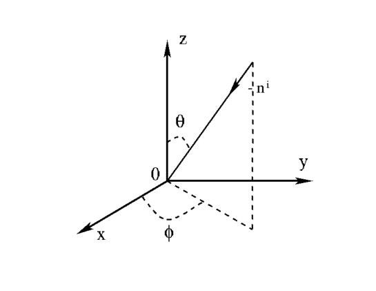
Figure 1: A gravitational wave is propagating along the spatial direction $\tilde{k}^{(0)i}\equiv-n^{i}$ to the observer located at the origin.

In the following, we shall set up the coordinates as follows LLSY10 : The observer is located at the origin with its proper time denoted by $\tau$ and world line $x^{\mu}(\tau)$. Denoting the time to receive the GW by $\tau_{r}$, this event will be recorded as $x^{\mu}(\tau)=\left(\tau_{r},\vec{o}\right)$. The emission time of the GW by an astrophysical source corresponds to the proper time $\tau_{e}$ of the observer with $x^{\mu}(\tau)=\left(\tau_{e},\vec{o}\right)$. Then, the GW will move along the null geodesics, described by $\tilde{x}^{\mu}(\tilde{\lambda})=\tilde{x}^{(0)\mu}(\tilde{\lambda})+\epsilon_{c}\tilde{x}^{(1)\mu}(\tilde{\lambda})$, which corresponds to the wave vector $\tilde{k}^{\mu}(\tilde{\lambda})=\tilde{k}^{(0)\mu}(\tilde{\lambda})+\epsilon_{c}\tilde{k}^{(1)\mu}(\tilde{\lambda})$, where $\tilde{x}^{(0)\mu}(\tilde{\lambda})=\left(\tilde{\lambda},(\tilde{\lambda}_{r}-\tilde{\lambda})n^{i}\right)$, and $\tilde{\lambda}_{r}$ is the moment when the GW arrives at the origin with $\tau(\tilde{\lambda}_{r})=\tau_{r}$.

The effects of the scalar and tensor perturbations are manifested from the perturbations of the null geodesics. Considering the fact $\tilde{\Gamma}^{(0)\mu}_{\nu\lambda}=0$ in the $\tilde{\gamma}_{\mu\nu}$ spacetime, we find that, to the first-order of $\epsilon_{c}$, $\tilde{k}^{(1)\mu}(\tilde{\lambda})$ is given by

$$\frac{d\tilde{k}^{(1)\mu}}{d\tilde{\lambda}}+\tilde{\Gamma}^{(1)\mu}_{\alpha\beta}\tilde{k}^{(0)\alpha}\tilde{k}^{(0)\beta}=0,$$ (4.29)

where $\tilde{\Gamma}^{(1)\mu}_{\alpha\beta}$ denotes the Christoffel symbols of the first-order of $\epsilon_{c}$. As mentioned previously, for the scalar perturbations, we shall not assume that $\psi=\phi$, that is, the trace of the anisotropic stress of the universe does not necessarily vanish, as shown by Eq.(A.15) in Appendix A. Then, for $\mu=0$ we find that

$$\frac{d}{d\lambda}\tilde{k}^{(1)0} = \partial_{\tau}(\phi+\psi)-2\frac{d\phi}{d\lambda}-\frac{1}{2}n^{k}n^{l}\partial_{\tau}H_{kl},~{}~{}~{}~{}~{}~{}~{}~{}~{}$$ (4.30)

where

$$\frac{d\Phi}{d\lambda}\equiv\left(\partial_{\tau}-n^{i}\partial_{i}\right)\Phi.$$ (4.31)

Thus, integrating Eq.(4.30) we find,

$$\tilde{k}^{(1)0}= -\left.\left(\phi+\psi\right)\right|^{\lambda}_{\lambda_{e}}+\frac{1}{2}n^{k}n^{l}H_{kl}|^{\lambda}_{\lambda_{e}}$$ (4.32)

$$-2\left.\phi\right|^{\lambda}_{\lambda_{e}}+I^{(s)}_{iSW}-\frac{1}{2}I^{(t)}_{iSW},~{}~{}~{}~{}~{}$$

where $I^{(s)}_{iSW}$ represents the gravitational iSW effect due to the cosmological scalar perturbations, and was first calculated in LLSY10 . The new term $I^{(t)}_{iSW}$ is the gravitational integrated effect due to the cosmological tensor perturbations. They are given, respectively, by

$$I^{(s)}_{iSW} \equiv \int^{\lambda}_{\lambda_{e}}\partial_{\tau}(\phi+\psi)d\lambda^{\prime},$$ (4.33)

$$I^{(t)}_{iSW} \equiv n^{k}n^{l}\int^{\lambda}_{\lambda_{e}}\partial_{\tau}H_{kl}d\lambda^{\prime}.$$ (4.34)

On the other hand, the spatial components of the wave-vector are given by,

$$\frac{d}{d\lambda}\tilde{k}^{(1)i}_{\parallel} = -n^{i}\Bigg{[}\partial_{\tau}(\phi+\psi)+\frac{d}{d\lambda}(\phi-\psi)$$ (4.35)

$$-\frac{1}{2}n^{k}n^{l}\Bigg{(}\frac{dH_{kl}}{d\lambda}+\partial_{\tau}H_{kl}\Bigg{)}\Bigg{]},~{}~{}~{}~{}~{}~{}$$

$$\frac{d}{d\lambda}\tilde{k}^{(1)i}_{\perp} = -\perp^{ij}\bigg{[}\partial_{j}(\phi+\psi)-n^{k}\frac{dH_{jk}}{d\lambda}$$ (4.36)

$$-\frac{1}{2}n^{k}n^{l}\partial_{j}H_{kl}\bigg{]},$$

where we had set $\tilde{k}^{(1)i}=\tilde{k}^{(1)i}_{\parallel}+\tilde{k}^{(1)i}_{\perp}$, with the parallel component of the spatial wave-vector being defined by $\tilde{k}^{(1)i}_{\parallel}=n^{i}n_{j}\tilde{k}^{(1)j}$, and the perpendicular component by $\tilde{k}^{(1)i}_{\perp}=\perp^{i}_{j}\tilde{k}^{(1)j}$. The projection operator $\perp^{i}_{j}$ is defined by $\perp^{i}_{j}=\delta^{i}_{j}-n^{i}n_{j}$, with $n_{i}\equiv\delta_{ik}n^{k}$. After integrations, the above two equations yield,

$$\tilde{k}^{(1)i}_{\parallel} = -n^{i}\Bigg{[}(\psi-\phi)|^{\lambda}_{\lambda_{e}}-\frac{1}{2}n^{k}n^{l}H_{kl}|^{\lambda}_{\lambda_{e}}$$ (4.37)

$$+I^{(s)}_{iSW}-\frac{1}{2}I^{(t)}_{iSW}\Bigg{]},$$

$$\tilde{k}^{(1)i}_{\perp} = -\perp^{ij}\Bigg{[}\int^{\lambda}_{\lambda_{e}}\partial_{j}(\phi+\psi)d\lambda^{\prime}-n^{k}H_{jk}|^{\lambda}_{\lambda_{e}}$$ (4.38)

$$-\frac{1}{2}n^{k}n^{l}\int^{\lambda}_{\lambda_{e}}\partial_{j}H_{kl}d\lambda^{\prime}\Bigg{]}.$$

The GW phase is then given by,

$$\frac{d\varphi}{d\lambda}=\phi+\psi-\frac{1}{2}n^{k}n^{l}\int^{\lambda}_{\lambda_{e}}H_{kl}d\lambda^{\prime},$$ (4.39)

which leads to

$$\delta\varphi=\varphi-\varphi_{e}= \int^{\lambda}_{\lambda_{e}}(\phi+\psi)d\lambda^{\prime}$$ (4.40)

$$-\frac{1}{2}n^{k}n^{l}\int^{\lambda}_{\lambda_{e}}H_{kl}d\lambda^{\prime}.$$

The frequency of the GW is defined as $\omega=-u^{\mu}k_{\mu}$, where $u^{\mu}$ is the 4-velocity of the fluid of the universe, given by Eqs.(Appendix A: Decompositions of cosmological perturbations and gauge choice) - (A.4), from which we find that the ratio of receiving and emitting frequencies is given by

$$\frac{\omega_{r}}{\omega_{e}}=\frac{1-\Upsilon}{1+z},$$ (4.41)

where $1+z\equiv a_{r}/a_{e}$, and

$$\Upsilon \equiv \phi|^{\lambda_{r}}_{\lambda_{e}}+v^{i}n_{i}+\frac{1}{2}n^{k}n^{l}H_{kl}|^{\lambda_{r}}_{\lambda_{e}}$$ (4.42)

$$-I^{(s)}_{iSW}|_{\lambda_{r}}+\frac{1}{2}I^{(t)}_{iSW}|_{\lambda_{r}}.$$

In addition, setting ${\cal{A}}={\cal{A}}^{(0)}(1+\epsilon_{c}\xi)$, from Eq.(4.15) we find

$$-2\frac{d\xi}{d\lambda}=\partial_{\tau}\tilde{k}^{(1)0}+\partial_{i}\tilde{k}^{(1)i}_{\parallel}+\partial_{i}\tilde{k}^{(1)i}_{\perp}+\tilde{\Gamma}^{(1)\mu}_{\mu\nu}\tilde{k}^{(0)\nu},~{}~{}~{}~{}$$ (4.43)

where

$$\partial_{\tau}\tilde{k}^{(1)0} = \partial_{\tau}\left(-2\phi+I^{(s)}_{iSW}-\frac{1}{2}I^{(t)}_{iSW}\right),$$

$$\partial_{i}\tilde{k}^{(1)i}_{\parallel} = \frac{d}{d\lambda}\left(\psi-\phi+I^{(s)}_{iSW}\right)$$

$$-\partial_{\tau}\left(\psi-\phi+I^{(s)}_{iSW}\right)$$

$$-\frac{1}{2}\frac{d}{d\lambda}\left(n^{k}n^{l}H_{kl}+I^{(t)}_{iSW}\right)$$

$$+\frac{1}{2}\partial_{\tau}\left(n^{k}n^{l}H_{kl}+I^{(t)}_{iSW}\right),$$

$$\partial_{i}\tilde{k}^{(1)i}_{\perp} = -\perp^{ij}\bigg{[}\int^{\lambda}_{\lambda_{e}}\partial_{i}\partial_{j}(\phi+\psi)d\lambda^{\prime}$$

$$-n^{k}\partial_{i}H_{kj}-\frac{1}{2}n^{k}n^{l}\int^{\lambda}_{\lambda_{e}}\partial_{i}\partial_{j}H_{kl}d\lambda^{\prime}\bigg{]},$$

$$\tilde{\Gamma}^{(1)\mu}_{\mu\nu}\tilde{k}^{(0)\nu} = \frac{d}{d\lambda}(\phi-3\psi).$$ (4.44)

Notice that in the last term, there are no contributions from the tensor perturbations. Collecting all of this together, Eq.(4.43) yields,

$$-2\frac{d\xi}{d\lambda} = -\partial_{\tau}(\phi+\psi)+\frac{d}{d\lambda}\left(-2\psi+I^{(s)}_{iSW}\right)$$ (4.45)

$$-\perp^{ij}\int^{\lambda}_{\lambda_{e}}\partial_{i}\partial_{j}(\phi+\psi)d\lambda^{\prime}$$

$$+\frac{1}{2}n^{k}n^{l}\partial_{\tau}H_{kl}-\frac{1}{2}\frac{d}{d\lambda}\left(n^{k}n^{l}H_{kl}+I^{(t)}_{iSW}\right)$$

$$+\perp^{ij}n^{k}\partial_{i}H_{jk}$$

$$+\frac{1}{2}\perp^{ij}n^{k}n^{l}\int^{\lambda}_{\lambda_{e}}\partial_{i}\partial_{j}H_{kl}d\lambda^{\prime},$$

which has the general solution,

$$\xi = -\psi|^{\lambda}_{\lambda_{e}}+\frac{1}{2}\perp^{ij}\int^{\lambda}_{\lambda_{e}}\int^{\lambda^{\prime}}_{\lambda_{e}}\partial_{i}\partial_{j}(\phi+\psi)d\lambda^{\prime}d\lambda^{\prime\prime}$$ (4.46)

$$-\frac{1}{2}n^{k}\Bigg{[}-\frac{1}{2}n^{l}H_{kl}|^{\lambda}_{\lambda_{e}}+\perp^{ij}\int^{\lambda}_{\lambda_{e}}\partial_{i}H_{jk}d\lambda^{\prime}$$

$$+\frac{1}{2}\perp^{ij}n^{l}\int^{\lambda}_{\lambda_{e}}\int^{\lambda^{\prime}}_{\lambda_{e}}\partial_{i}\partial_{j}H_{kl}d\lambda^{\prime}d\lambda^{\prime\prime}\Bigg{]}.$$

In terms of the gravitational tensorial iSW effect defined by Eq.(4.34), the above expression can be written in the form,

$$\xi = \left.\left(\psi-\frac{1}{4}n^{k}n^{l}H_{kl}\right)\right|^{\lambda}_{\lambda_{e}}+\frac{1}{2}I^{(t)}_{iSW}$$ (4.47)

$$-\frac{1}{4}\perp^{ij}\int^{\lambda}_{\lambda_{e}}\int^{\lambda^{\prime}}_{\lambda_{e}}\partial_{i}\partial_{j}\Bigg{[}n^{k}n^{l}H_{kl}-2\left(\phi+\psi\right)\Bigg{]}d\lambda^{\prime\prime}d\lambda^{\prime}$$

$$-\frac{1}{2}n^{k}\int^{\lambda}_{\lambda_{e}}\partial^{l}H_{kl}d\lambda^{\prime}.$$

Combining all of our results together, we are at the point to construct the gravitational waveform through Eq.(4.2), from which we find that

$$h_{\mu\nu} = \chi_{\mu\nu}-\frac{1}{2}\chi\gamma_{\mu\nu}=e_{\mu\nu}\tilde{h},$$

$$\tilde{h} \equiv \mathcal{A}e^{i\varphi}=\frac{(1+z)\mathcal{Q}}{d_{L}}(1+\xi)e^{i(\varphi_{e}+\delta\varphi)},$$ (4.48)

where $\delta\varphi$ and $\xi$ are given, respectively, by Eqs.(4.40) and (4.47), and $d_{L}\equiv(1+z){\cal{R}}$ is the luminosity distance. Note that in writing the expression for the response function $\tilde{h}$ we had set $\epsilon=1$.

For a binary system, we have PW14 ; LLSY10 ,

$$\mathcal{Q} = \mathcal{M}_{e}\left(\pi f_{e}\mathcal{M}_{e}\right)^{2/3},$$

$$\varphi_{e} = \varphi_{c}-\left(\pi f_{e}\mathcal{M}_{e}\right)^{-5/3},$$ (4.49)

where $\mathcal{M}_{e}$ and $f_{e}$ denote, respectively, the intrinsic chirp mass and frequency of the binary, and $\phi_{c}$ is the value of the phase at the merge, at which we have $f=\infty$. Therefore, the function $\tilde{h}$ for a binary system can be cast in the form,

$$\tilde{h}=\frac{\mathcal{M}_{r}}{D_{L}}(\pi f_{r}\mathcal{M}_{r})^{2/3}e^{i(\varphi_{e}+\delta\varphi)},$$ (4.50)

where the modified luminosity distance $D_{L}$ and the chirp mass ${\cal{M}}_{r}$ measured by the observer are given, respectively, by

$$D_{L} \equiv \frac{d_{L}}{1-\Upsilon-\xi},\quad\mathcal{M}_{r}\equiv\left(\frac{1+z}{1-\Upsilon}\right)\mathcal{M}_{e},$$ (4.51)

where $\Upsilon$ is given by Eq.(4.42).

V Conclusions

In this paper, we have systematically studied GWs, which are first produced by some remote compact astrophysical sources, and then propagate in our inhomogeneous universe through cosmic distances before arriving at the detectors. Such GWs will carry valuable information of both their sources and the cosmological expansion and inhomogeneities of the universe, whereby a completely new window to explore our universe by using GWs is opened. As the third generation (3G) detectors, such as the space-based ones, LISA PAS17 , TianQin TianQin , Taiji Taiji , DECIGO DECIGO , and the ground-based ones, ET ET and CE CE , are able to detect GWs emitted from such sources as far as at the redshift $z\simeq 100$ HE19 (See also Footnote 1), it is very important and timely to carry out such studies systematically. Such studies were already initiated some years ago LLSY10 ; BRBM17 ; BCST17 in the framework of Einstein’s theory, and more recently in scalar-tensor theories Garoffolo19 ; DFL20a ; DFL20b ; EZ20 ; EZ20 .

In this paper, in order to characterize effectively such systems, we first introduced three scales, $\lambda,\;L_{c}$ and $L$, which represent, respectively, the typical wavelength of the GWs, the scale of the cosmological perturbations, and the size of our observable universe. For GWs to be detected by the current and foreseeable (both ground- and space-based) detectors, in Sec. II we showed that the relation

$$\lambda\ll L_{c}\ll L,$$ (5.1)

is always true, that is, such GWs can be well approximated as high frequency GWs, for which the general formulas were already developed by Isaacson more than half century ago Isaacson68a ; Isaacson68b .

However, Isaacson considered only the case where the background is vacuum, while in LLSY10 ; BRBM17 ; BCST17 only the cosmological scalar perturbations were considered. In this paper, we considered the most general case in which the background also includes the cosmological tensor perturbations. The inclusion of the latter is important, as now one of the main goals of cosmological observations is the primordial GWs (the tensor perturbations) CMB-S4 . In the non-vacuum case, (in Sec. II) we showed explicitly that the conditions

$$\left|h_{\mu\nu}\right|\ll 1,\quad\epsilon\ll\epsilon_{c}\ll 1,$$ (5.2)

must hold, in order for the backreaction of the GWs to the background to be neglected, and the linearized Einstein field equations given by Eq.(2.41) to hold, where the total metric of the spacetime is expanded as $g_{\mu\nu}=\gamma_{\mu\nu}+\epsilon h_{\mu\nu}$, with $\gamma_{\mu\nu}(\equiv\bar{\gamma}_{\mu\nu}+\epsilon_{c}\hat{\gamma}_{\mu\nu})$ representing the background.

In Sec. III, we considered the gauge choices, and found that the three different gauge conditions, spatial, traceless, and Lorenz, given respectively by Eqs.(1.4) - (1.6), can be still imposed simultaneously, even when both the cosmological scalar and tensor perturbations are present, as long as the GWs can be approximated as the high-frequency GWs. However, by imposing only the spatial gauge (1.4), the linearized Einstein field equations (2.41) are explicitly given in Appendix B. If $\chi_{\mu\nu}$ is decomposed into two parts,

$$\chi_{\mu\nu}=\chi_{\mu\nu}^{(0)}+\epsilon_{c}\chi_{\mu\nu}^{(1)}+{\cal{O}}\left(\epsilon_{c}^{2}\right),$$ (5.3)

the field equations for $\chi_{\mu\nu}^{(1)}$ are given explicitly in Appendix C.

As an application of our general formulas, developed in Secs. II and III, in Sec. IV we studied the GWs by using the geometrical optics approximation,

$$\chi_{\alpha\beta}=e_{\alpha\beta}{\cal{A}}e^{i\varphi/\epsilon},$$ (5.4)

where $e_{\alpha\beta}$ represents the polarization tensor, ${\cal{A}}$ and $\varphi$ denote, respectively, the amplitude and phase of the GWs. We showed explicitly that even when both the cosmological scalar and tensor perturbations are present, such GWs are still propagating along null geodesics, and the current of gravitons moving along the null geodesics is conserved, and the polarization tensor is parallel-transported, i.e.,

$$k^{\lambda}\nabla_{\lambda}k^{\mu}=0,\quad k^{\lambda}\nabla_{\lambda}e_{\alpha\beta}=0,\quad\nabla^{\lambda}J_{\lambda}=0,$$ (5.5)

where $k_{\mu}\equiv\nabla_{\mu}\varphi,\;J_{\mu}\equiv{\cal{A}}^{2}k_{\mu}$. In fact, these are true for any curved background, provided that: (a) the GWs can be considered as high-frequency GWs; and (b) the geometrical optics approximation are valid MTW73 .

With these remarkable features, we calculated the effects of the cosmological scalar and tensor perturbations on the amplitude ${\cal{A}}$ and phase $\varphi$, given by Eqs.(4.40), (4.47) and (IV.2). Restricting to GWs produced by a binary system, the effects of the cosmological perturbations, both scalar and tensor, on the luminosity distance and the chirp mass are given explicitly by Eq.(4.51), which represent a natural generalization of the results obtained in LLSY10 ; BRBM17 ; BCST17 to the case in which the cosmological tensor perturbations are also present.

It should be noted that in cosmology the effects of the scalar and tensor perturbations of the homogeneous universe on the luminosity distances were studied in SW67 ; PC96 and DD12 . Since in the geometrical optics approximations both GWs and electromagnetic waves (EWs) are all moving alone the null geodesics, the effects of the cosmological scalar perturbations on the luminosity distance of GWs carried out in LLSY10 should be the same as that obtained in SW67 ; PC96 for EWs, while the ones of the cosmological tensor perturbations carried out in this paper should be the same as that obtained in DD12 for EWs. However, the calculations of the GW phase are new. This is mainly due to the fact that the detection of GWs depends not only their amplitudes but also their phases MM16 , while the phases of EWs in cosmology do not play a significant role SD03 .

The applications of our general formulas developed in this paper to other studies are immediate, including the gravitational analogue of the electromagnetic Faraday rotations Wang91 ; Wang20 ; HFZ19 ; FSW20 , and their detections by the space- and ground-based detectors. We wish to return to these important issues in other occasions soon.

It would be also very important to extend such studies to include the relations between the GWs and their sources, high-order corrections to the geometrical optics approximations, and more interesting the non-high frequency GWs.

Appendix A: Decompositions of cosmological perturbations and gauge choice

Following Malik01 ; DB09 , the linear perturbations $\hat{\gamma}_{\mu\nu}$ can be decomposed into scalar, vector and tensor modes, and given explicitly by Eq.(2.45).

The energy-momentum tensor ${T_{\mu\nu}}^{(0)}$ of a fluid takes the form Malik01 ,

$${T^{\mu}_{\nu}}^{(0)}=\left(\rho+p\right)u^{\mu}u_{\nu}+p\delta^{\mu}_{\nu}+\pi^{\mu}_{\nu},$$ (A.1)

where ${u}^{\mu}$ is the 4-velocity of the fluid, $\rho$ and ${p}$ are its energy density and isotropic pressure, respectively, and $\pi^{\mu}_{\nu}$ is the anisotropic stress tensor, which has only spatial components, i.e., $\pi^{\mu}_{0}=0$. Setting

$$\rho = \bar{\rho}+\epsilon_{c}\delta\rho,\quad p=\bar{p}+\epsilon_{c}\delta p,$$

$$u^{\mu} = \bar{u}^{\mu}+\epsilon_{c}\delta{u}^{\mu},$$ (A.2)

where $\bar{u}^{\mu}=a^{-1}\delta_{\eta}^{\mu}$ is the 4-velocity of the fluid of the homogenous and isotropic universe, and $\bar{\rho}$ and $\bar{p}$ are its energy density and isotropic pressure, respectively, we find that $\delta{u}^{\mu}$ can be decomposed as

$$\delta u^{\mu}=\frac{1}{a}\left(-\phi,\partial^{i}v+v^{i}\right),$$ (A.3)

where $\partial_{i}v^{i}=0$. Then, from $u_{\mu}\equiv\gamma_{\mu\nu}u^{\nu}=\bar{u}_{\mu}+\epsilon_{c}\delta{u}_{\mu}$, we find that

$$\delta u_{\mu}={a}\left(-\phi,\partial_{i}v+\partial_{i}B+v_{i}-S_{i}\right),$$ (A.4)

which leads to $u^{\mu}u_{\mu}=-1+{\cal{O}}\left(\epsilon_{c}^{2}\right)$, as expected.

On the other hand, setting $\pi^{j}_{i}=\epsilon_{c}\hat{\pi}^{j}_{i}$, similar to $\hat{\gamma}_{\mu\nu}$, the anisotropic stress tensor $\hat{\pi}^{j}_{i}$ can be decomposed into scalar, vector and tensor modes,

$$\hat{\pi}^{j}_{i} = \left(\partial^{j}\partial_{i}-\frac{1}{3}\delta^{j}_{i}\partial^{2}\right)\Pi+\frac{1}{2}\left(\partial_{i}\Pi^{j}+\partial^{j}\Pi_{i}\right)+\Pi^{j}_{\;\;i},$$

where $\partial_{i}\Pi^{i}=0=\Pi^{i}_{\;\;i}$, $\partial_{j}\Pi^{j}_{\;\;i}=0$, $\Pi^{i}\equiv\delta^{ik}\Pi_{k},\;\Pi^{i}_{\;\;j}\equiv\delta^{ik}\Pi_{kj}$, $\partial^{2}\equiv\partial^{i}\partial_{i}$, etc. Then, we find that

$${T^{0}_{\;\;\;0}}^{(0)} = -\bar{\rho}-\epsilon_{c}\delta\rho,$$

$${T^{0}_{\;\;\;i}}^{(0)} = \epsilon_{c}\left(\bar{\rho}+\bar{p}\right)\left[\partial_{i}(v+B)+v_{i}-S_{i}\right],$$

$${T^{i}_{\;\;\;0}}^{(0)} = -\epsilon_{c}\left(\bar{\rho}+\bar{p}\right)\left(\partial^{i}v+v^{i}\right),$$

$${T^{i}_{\;\;\;j}}^{(0)} = \bar{p}\delta^{i}_{j}+\epsilon_{c}\left(\delta{p}\delta^{i}_{j}+\hat{\pi}^{i}_{j}\right).$$ (A.6)

V.1 Gauge Transformations of Cosmological Perturbations

Considering the gauge transformations,

$$\tilde{\eta}=\eta+\epsilon_{c}\zeta^{0},\quad\tilde{x}^{i}=x^{i}+\epsilon_{c}\left(\partial^{i}\zeta+{\zeta}^{i}\right),$$ (A.7)

where $\partial_{i}{\zeta}^{i}=0$, we find that

$$\tilde{\phi} = \phi-{\cal{H}}\zeta^{0}-{\zeta^{0}}^{\prime},\;\;\tilde{\psi}=\psi+{\cal{H}}\zeta^{0},$$

$$\tilde{B} = B+\zeta^{0}-\zeta^{\prime},\;\;\tilde{E}=E-\zeta,$$

$$\tilde{\delta\rho} = \delta\rho-\zeta^{0}\bar{\rho}^{\prime},\;\;\tilde{\delta{p}}=\delta{p}-\zeta^{0}\bar{p}^{\prime},$$

$$\tilde{v} = v+\zeta^{\prime},$$ (A.8)

$$\tilde{F}_{i} = F_{i}-\zeta_{i},\;\;\tilde{S}_{i}=S_{i}+\zeta_{i}^{\prime},$$

$$\tilde{v}^{i} = v^{i}+{\zeta^{i}}^{\prime},$$ (A.9)

$$\tilde{H}_{ij} = H_{ij},\quad\tilde{\pi}^{i}_{j}=\pi^{i}_{j},$$ (A.10)

where ${\cal{H}}\equiv a^{\prime}/a$ with $a^{\prime}\equiv da/d\eta$. From the above gauge transformations we can see that the following quantities are gauge-invariant,

$$\Phi \equiv \phi+{\cal{H}}\left(B-E^{\prime}\right)+\left(B-E^{\prime}\right)^{\prime},$$

$$\Psi \equiv \psi-{\cal{H}}\left(B-E^{\prime}\right),$$

$$\Phi_{i} \equiv S_{i}+F_{i}^{\prime}.$$ (A.11)

On the other hand, if we choose $\zeta=E,\;\zeta^{0}=E^{\prime}-B$ and $\zeta_{i}=F_{i}$, we have

$$\tilde{B}=\tilde{E}=0,\quad\tilde{F}_{i}=0,$$ (A.12)

in which the gauge is completely fixed. This is often referred to as the Newtonian gauge. Then, we are left with six scalars, $(\phi,\psi,v,\delta\rho,\delta{p},\Pi)$, two vectors, $(S_{i},v_{i})$, and two tensors, $(H_{ij},\Pi_{ij})$. However, the vector part decreases rapidly with the expansion of the universe, so we can safely set them to zero Malik01 ; DB09 ,

$$S_{i}=F_{i}=v_{i}=\Pi_{i}=0.$$ (A.13)

Then, for the scalar perturbations, there are six-independent equations, given, respectively, by Malik01 ,

$$\psi^{\prime\prime}+2{\cal{H}}\psi^{\prime}+{\cal{H}}\phi^{\prime}+\left(2{\cal{H}}^{\prime}+{\cal{H}}^{2}\right)\phi$$

$$~{}~{}~{}~{}~{}~{}~{}~{}~{}~{}~{}~{}~{}~{}~{}~{}=4\pi Ga^{2}\left(\delta p+\frac{2}{3}\nabla^{2}\Pi\right),$$ (A.14)

$$\psi-\phi=8\pi Ga^{2}\Pi,$$ (A.15)

$$3{\cal{H}}\left(\psi^{\prime}+{\cal{H}}\phi\right)-\nabla^{2}\psi=-4\pi Ga^{2}\delta\rho,$$ (A.16)

$$\psi^{\prime}+{\cal{H}}\phi=-4\pi Ga^{2}\left(\bar{\rho}+\bar{p}\right)v,$$ (A.17)

$$\delta\rho^{\prime}+3{\cal{H}}\left(\delta\rho+\delta p\right)=\left(\bar{\rho}+\bar{p}\right)\left(3\psi^{\prime}-\nabla^{2}v\right),~{}~{}~{}~{}~{}$$ (A.18)

$$\left[\left(\bar{\rho}+\bar{p}\right)v\right]^{\prime}+\delta{p}+\frac{2}{3}\nabla^{2}\Pi$$

$$~{}~{}~{}~{}~{}~{}~{}~{}~{}~{}~{}~{}~{}~{}~{}~{}=-\left(\bar{\rho}+\bar{p}\right)\left(\phi+4{\cal{H}}v\right).$$ (A.19)

Note that Eqs.(V.1) and (A.15) are obtained from the linearized (i, j)-components of the Einstein field equations, and Eqs.(A.16) and (A.17) are the energy and momentum constraints, while Eqs.(A.18) and (V.1) are obtained from the conservation of the energy-momentum tensor.

For the tensor perturbations, we have

$$H_{ij}^{\prime\prime}+2{\cal{H}}H_{ij}^{\prime}-\nabla^{2}H_{ij}=16\pi Ga^{2}\Pi_{ij},$$ (A.20)

which is obtained from the equations $\delta{G^{(0)}}^{i}_{j}=\kappa\delta{T^{(0)}}^{i}_{j}$.

It must be noted that in writing the linearized field equations, (V.1) - (A.20), we had implicitly assumed that the quadratic terms $\epsilon_{c}^{2}\hat{R}^{(2)}_{\mu\nu}(\hat{\gamma})\simeq{\cal{O}}(\hat{\gamma}^{2})\ll 1$, which is equivalent to

$$\hat{\gamma}\ll 1,$$ (A.21)

where $\hat{R}^{(2)}_{\mu\nu}(\hat{\gamma})$ is given by Eq.(II.3) with the replacement $\left(h_{\mu\nu},\nabla_{\alpha}\right)\rightarrow\left(\hat{\gamma}_{\mu\nu},\bar{\nabla}_{\alpha}\right)$. Otherwise, these quadratic terms cannot be neglected from the Einstein field equations for the background spacetimes,

$$\bar{G}_{\mu\nu}(\bar{\gamma})+\epsilon_{c}\hat{G}_{\mu\nu}(\hat{\gamma})+\epsilon_{c}^{2}\hat{G}^{(2)}_{\mu\nu}(\hat{\gamma})=\kappa T^{(0)}_{\mu\nu},$$ (A.22)

where

$$\bar{G}_{\mu\nu}(\bar{\gamma}) \simeq {\cal{O}}(1),\quad\epsilon_{c}\hat{G}_{\mu\nu}(\hat{\gamma})\simeq{\cal{O}}(\hat{\gamma}/\epsilon_{c}),$$

$$\epsilon_{c}^{2}\hat{G}^{(2)}_{\mu\nu}(\hat{\gamma}) \simeq {\cal{O}}(\hat{\gamma}^{2}),$$ (A.23)

as can be seen from Eq.(II.3).

Appendix B: Field Equations for $\chi_{ij}$

In this Appendix, we shall calculate all the components of the quantities appearing in the field equations (3.22) for $\chi_{\alpha\beta}$, by imposing only the spatial gauge,

$$\chi_{0\mu}=0.$$

In particular, to calculate the non-vanishing components of the tensor ${\cal{G}}_{\alpha\beta}$, we first note that

$$\chi^{ij}\equiv\gamma^{i\mu}\gamma^{j\nu}\chi_{\mu\nu}=\gamma^{ik}\gamma^{jl}\chi_{kl}=\frac{1}{a^{2}}\Big{\{}\delta^{ik}\delta^{jl}+\epsilon_{c}\left[4\psi\delta^{ik}\delta^{jl}-\left(\delta^{ik}H^{jl}+\delta^{jl}H^{ik}\right)\right]\Big{\}}\hat{\chi}_{kl},$$

$$\gamma_{ij}\chi^{ij}=\hat{\chi}+\epsilon_{c}\left(2\psi\hat{\chi}-H^{kl}\hat{\chi}_{kl}\right),\quad\chi\equiv\gamma^{\mu\nu}\chi_{\mu\nu}=\gamma^{ij}\chi_{ij}=\gamma_{ij}\chi^{ij},$$

$$\gamma_{ij}\chi^{ik}\hat{\pi}^{j}_{k}=\Big{[}\hat{\pi}^{kl}+\epsilon_{c}\left(2\psi\hat{\pi}^{kl}-\hat{\pi}^{k}_{m}H^{ml}\right)\Big{]}\hat{\chi}_{kl},$$

$$\chi^{\gamma\sigma}{T_{\gamma\sigma}}^{(0)}-\frac{1}{2}\chi T^{(0)}=\frac{1}{2}\left(\bar{\rho}-\bar{p}\right)\hat{\chi}+\frac{1}{2}\epsilon_{c}\Big{[}\left(\bar{\rho}-\bar{p}\right)\left(2\psi\hat{\chi}-H^{kl}\hat{\chi}_{kl}\right)+\left(\delta\rho-\delta p\right)\hat{\chi}+2\hat{\pi}^{kl}\hat{\chi}_{kl}\Big{]},$$ (B.1)

where $\hat{\chi}\equiv\delta^{ij}\hat{\chi}_{ij}$, $\chi_{ij}\equiv a^{2}\hat{\chi}_{ij}$, $\hat{\pi}_{ij}\equiv\delta_{ik}\hat{\pi}^{k}_{j}$, etc. Then, from Eq.(2.42) we find that

$${\cal{F}}_{00} = -\frac{a^{2}}{2}\Bigg{\{}\left(\bar{\rho}-\bar{p}\right)\hat{\chi}+\epsilon_{c}\Bigg{[}\left(\bar{\rho}-\bar{p}\right)\Big{(}2\left(\psi+\phi\right)\hat{\chi}-H^{kl}\hat{\chi}_{kl}\Big{)}+\left(\delta\rho-\delta p\right)\hat{\chi}+2\hat{\pi}^{kl}\hat{\chi}_{kl}\Bigg{]}\Bigg{\}},$$

$${\cal{F}}_{0i} = -a^{2}\epsilon_{c}\left(\bar{\rho}+\bar{p}\right)\hat{\chi}_{ik}\partial^{k}v,$$

$${\cal{F}}_{ij} = \frac{1}{2}a^{2}\Big{[}4\bar{p}\hat{\chi}_{ij}+\left(\bar{\rho}-\bar{p}\right)\hat{\chi}\delta_{ij}\Big{]}+\frac{1}{2}a^{2}\epsilon_{c}\Bigg{\{}\Big{[}4\delta p\hat{\chi}_{ij}+\left(\delta\rho-\delta p\right)\hat{\chi}\delta_{ij}\Big{]}+\left(\bar{\rho}-\bar{p}\right)\left(\hat{\chi}H_{ij}-H^{kl}\hat{\chi}_{kl}\delta_{ij}\right)$$ (B.2)

$$+2\left(\hat{\pi}^{k}_{i}\hat{\chi}_{jk}+\hat{\pi}^{k}_{j}\hat{\chi}_{ik}+\hat{\pi}^{kl}\hat{\chi}_{kl}\delta_{ij}\right)\Bigg{\}}.$$

In addition, the non-vanishing (independent) components of the Riemann tensor,

$${R_{\mu\nu\alpha\beta}}^{(0)}=\bar{R}_{\mu\nu\alpha\beta}+\epsilon_{c}\hat{R}_{\mu\nu\alpha\beta},$$ (B.3)

are given, respectively, by

$$\bar{R}_{0i0j} = a^{2}\left({\cal{H}}^{2}-\frac{a^{\prime\prime}}{a}\right)\delta_{ij},\quad\quad\bar{R}_{minj}=a^{2}{\cal{H}}^{2}\left(\delta_{ij}\delta_{mn}-\delta_{in}\delta_{mj}\right),$$ (B.4)

and

$$\hat{R}_{0i0j} = a^{2}\Bigg{\{}\phi_{,ij}+{\cal{H}}\phi^{\prime}\delta_{ij}+\Bigg{[}\left(\psi^{\prime\prime}+{\cal{H}}\psi^{\prime}\right)+2\left(\frac{a^{\prime\prime}}{a}-{\cal{H}}^{2}\right)\psi\Bigg{]}\delta_{ij}-\frac{1}{2}\Bigg{[}\left({H_{ij}}^{\prime\prime}+{\cal{H}}{H_{ij}}^{\prime}\right)+2\left(\frac{a^{\prime\prime}}{a}-{\cal{H}}^{2}\right)H_{ij}\Bigg{]}\Bigg{\}},$$

$$\hat{R}_{0ijk} = a^{2}\Big{[}{\cal{H}}\left(\phi_{,j}\delta_{ik}-\phi_{,k}\delta_{ij}\right)+\left(\psi_{,j}^{\prime}\delta_{ik}-\psi_{,k}^{\prime}\delta_{ij}\right)+\frac{1}{2}\left(H_{ij,k}^{\prime}-H_{ik,j}^{\prime}\right)\Big{]},$$

$$\hat{R}_{ijkl} = -2a^{2}{\cal{H}}^{2}\phi\left(\delta_{ik}\delta_{jl}-\delta_{il}\delta_{jk}\right)-a^{2}\Big{[}\left(\delta_{jk}\psi_{,il}+\delta_{il}\psi_{,jk}-\delta_{ik}\psi_{,jl}-\delta_{jl}\psi_{,ik}\right)+2{\cal{H}}\left(\psi^{\prime}+2{\cal{H}}\psi\right)\left(\delta_{ik}\delta_{jl}-\delta_{il}\delta_{jk}\right)\Big{]}$$ (B.5)

$$+\frac{1}{2}a^{2}\Bigg{\{}\left(H_{jk,il}+H_{il,jk}-H_{ik,jl}-H_{jl,ik}\right)-{\cal{H}}\Big{[}\delta_{il}\left(H_{jk}^{\prime}+2{\cal{H}}H_{jk}\right)+\delta_{jk}\left(H_{il}^{\prime}+2{\cal{H}}H_{il}\right)$$

$$~{}~{}~{}~{}~{}~{}~{}~{}~{}~{}-\delta_{jl}\left(H_{ik}^{\prime}+2{\cal{H}}H_{ik}\right)-\delta_{ik}\left(H_{jl}^{\prime}+2{\cal{H}}H_{jl}\right)\Big{]}\Bigg{\}}.$$

Hence, we find that

$$2{R_{0i0j}}^{(0)}\chi^{ij} = 2\bigg{(}\frac{a^{\prime\prime}}{a}-\mathcal{H}^{2}\bigg{)}\hat{\chi}+\epsilon_{c}\bigg{\{}2\left(\partial^{i}\partial^{j}\phi\right)\hat{\chi}_{ij}+2\mathcal{H}\phi^{\prime}\hat{\chi}+2\big{(}\psi^{\prime\prime}+\mathcal{H}\psi^{\prime}\big{)}\hat{\chi}-4\bigg{(}\frac{a^{\prime\prime}}{a}-\mathcal{H}^{2}\bigg{)}\psi\hat{\chi}$$

$$~{}~{}~{}~{}~{}~{}~{}~{}~{}~{}~{}~{}~{}~{}~{}~{}~{}~{}~{}~{}~{}~{}~{}~{}~{}~{}~{}~{}-\big{(}{H^{ij}}^{\prime\prime}+\mathcal{H}{H^{ij}}^{\prime}\big{)}\hat{\chi}_{ij}+2\bigg{(}\frac{a^{\prime\prime}}{a}-\mathcal{H}^{2}\bigg{)}H^{ij}\hat{\chi}_{ij}\bigg{\}},$$

$$2{R_{0jik}}^{(0)}\chi^{jk} = 2\epsilon_{c}\Bigg{\{}\mathcal{H}\left[\left(\partial_{i}\phi\right)\hat{\chi}-\left(\partial^{k}\phi\right)\hat{\chi}_{ik}\right]+\left(\partial_{i}\psi^{\prime}\right)\hat{\chi}-\left(\partial^{k}\psi^{\prime}\right)\hat{\chi}_{ik}+\frac{1}{2}\left[\left(\partial^{k}{H^{j}_{i}}^{\prime}\right)-\left(\partial_{i}{H^{jk}}^{\prime}\right)\right]\hat{\chi}_{jk}\Bigg{\}},$$

$$2{R_{ikjl}}^{(0)}\chi^{kl} = 2\mathcal{H}^{2}\big{(}\delta_{ij}\hat{\chi}-\hat{\chi}_{ij}\big{)}+\epsilon_{c}\bigg{\{}4\mathcal{H}^{2}\phi\left(\hat{\chi}_{ij}-\hat{\chi}\delta_{ij}\right)+4\mathcal{H}\psi^{\prime}\left(\hat{\chi}_{ij}-\hat{\chi}\delta_{ij}\right)$$ (B.6)

$$+2\Big{[}\left(\partial_{i}\partial_{j}\psi\right)\hat{\chi}+\left(\partial^{k}\partial^{l}\psi\right)\hat{\chi}_{kl}\delta_{ij}-\left(\partial^{k}\partial_{i}\psi\right)\hat{\chi}_{jk}-\left(\partial^{k}\partial_{j}\psi\right)\hat{\chi}_{ik}\Big{]}$$

$$-2\mathcal{H}^{2}H^{kl}\hat{\chi}_{kl}\delta_{ij}+2\mathcal{H}^{2}H_{ij}\hat{\chi}-2\mathcal{H}{H^{k}_{(i}}^{\prime}\hat{\chi}_{j)k}+\mathcal{H}{H_{ij}}^{\prime}\hat{\chi}+\mathcal{H}{H^{kl}}^{\prime}\hat{\chi}_{kl}\delta_{ij}$$

$$+\left(2\partial_{(i}\partial^{l}H^{k}_{j)}-\partial^{k}\partial^{l}H_{ij}-\partial_{i}\partial_{j}H^{kl}\right)\hat{\chi}_{kl}\bigg{\}}.$$

On the other hand, similar to the above expression, writing $\square\chi_{\alpha\beta}$ in the form,

$$\square\chi_{\alpha\beta} \equiv \bar{\square}\chi_{\alpha\beta}+\epsilon_{c}\hat{\square}\chi_{\alpha\beta},$$ (B.7)

we find they are given, respectively, by

$$\bar{\square}\chi_{00} = 2{\cal{H}}^{2}\hat{\chi},\quad\bar{\square}\chi_{0i}=-2{\cal{H}}\partial^{j}\hat{\chi}_{ij},\quad\bar{\square}\chi_{ij}=-{\hat{\chi}}_{ij}^{\prime\prime}-2{\cal{H}}{\hat{\chi}}_{ij}^{\prime}+\partial^{2}\hat{\chi}_{ij}+2{{\cal{H}}^{2}}\hat{\chi}_{ij},$$ (B.8)

and

$$\hat{\square}\chi_{00} = -2{\cal{H}}\Big{[}2\left(\psi^{\prime}-{\cal{H}}\psi\right)\hat{\chi}-\left({H^{ij}}^{\prime}-{\cal{H}}H^{ij}\right)\hat{\chi}_{ij}\Big{]},$$

$$\hat{\square}\chi_{0i} = \left(\partial^{j}\phi^{\prime}\right)\hat{\chi}_{ij}+2\left(\partial^{j}\phi\right)\left(\hat{\chi}_{ij}^{\prime}+{\cal{H}}\hat{\chi}_{ij}\right)+\left(\partial^{j}\psi^{\prime}\right)\hat{\chi}_{ij}+2\left(\psi^{\prime}-2{\cal{H}}\psi\right)\partial^{j}\hat{\chi}_{ij}+2{\cal{H}}\left[\left(\partial^{j}\psi\right)\hat{\chi}_{ij}-\left(\partial_{i}\psi\right)\hat{\chi}\right]$$

$$-\left({H^{jk}}^{\prime}-2{\cal{H}}H^{jk}\right)\partial_{k}\hat{\chi}_{ij}+{\cal{H}}\left(\partial_{i}H^{jk}\right)\hat{\chi}_{jk},$$

$$\hat{\square}\chi_{ij} = 2\phi\hat{\chi}_{ij}^{\prime\prime}+\left(\phi^{\prime}+4{\cal{H}}\phi\right)\hat{\chi}_{ij}^{\prime}+\left(\partial^{k}\phi\right)\partial_{k}\hat{\chi}_{ij}-4{\cal{H}}^{2}\phi\hat{\chi}_{ij}$$ (B.9)

$$+2\psi\partial^{2}\hat{\chi}_{ij}+4\partial_{(i}\psi\partial^{k}\hat{\chi}_{j)k}+3\left(\partial^{k}\psi\right)\partial_{k}\hat{\chi}_{ij}-4\left(\partial^{k}\psi\right)\partial_{(i}\hat{\chi}_{j)k}+2\partial^{k}\partial_{(i}\psi\hat{\chi}_{j)k}+2\left(\partial^{2}\psi\right)\hat{\chi}_{ij}$$

$$-2\partial_{(i}\partial^{k}\psi\hat{\chi}_{j)k}-\psi^{\prime}{\hat{\chi}_{ij}}^{\prime}-2\left(\psi^{\prime\prime}+4{\cal{H}}\psi^{\prime}\right)\hat{\chi}_{ij}$$

$$-H^{kl}\partial_{k}\partial_{l}\hat{\chi}_{ij}-2\partial^{l}H^{k}\hskip 0.28453pt_{(i}\partial_{l}\hat{\chi}_{j)k}-2\partial_{(i}H^{kl}\partial_{l}\hat{\chi}_{j)k}+2\partial^{k}H_{(i}\hskip 0.28453pt^{l}\partial_{l}\hat{\chi}_{j)k}+2H^{k}\hskip 0.28453pt_{(i}\hskip 0.28453pt{}^{\prime}\hat{\chi}_{j)k}^{\prime}+H^{k}\hskip 0.28453pt_{(i}\hskip 0.28453pt{}^{\prime\prime}\hat{\chi}_{j)k}$$

$$+4\mathcal{H}H^{k}\hskip 0.28453pt_{(i}\hskip 0.28453pt{}^{\prime}\hat{\chi}_{j)k}-\partial^{2}H^{k}\hskip 0.28453pt_{(i}\hat{\chi}_{j)k},$$

where $2\partial^{k}\partial_{(i}\psi\hat{\chi}_{j)k}\equiv\left(\partial^{k}\partial_{i}\psi\right)\hat{\chi}_{jk}+\left(\partial^{k}\partial_{j}\psi\right)\hat{\chi}_{ik}$, that is, the partial derivative acts only to the first function. The same is true for other terms, for example, $2\partial^{l}H^{k}\hskip 0.28453pt_{(i}\partial_{l}\hat{\chi}_{j)k}\equiv\left(\partial^{l}H^{k}\hskip 0.28453pt_{i}\right)\partial_{l}\hat{\chi}_{jk}+\left(\partial^{l}H^{k}\hskip 0.28453pt_{j}\right)\partial_{l}\hat{\chi}_{ik}$.

On the other hand, defining

$${\cal{G}}_{\alpha\beta}^{(1)}\equiv\gamma_{\alpha\beta}\nabla^{\gamma}\nabla^{\delta}\chi_{\gamma\delta},$$ (B.10)

we find that

$${\cal{G}}_{00}^{(1)} = -{\cal{G}}^{(1)}_{0}-\epsilon_{c}\left(2\phi{\cal{G}}^{(1)}_{0}+{\cal{G}}^{(1)}_{1}\right),\quad{\cal{G}}_{0i}^{(1)}={\cal{G}}_{i0}^{1}=0,$$

$${\cal{G}}_{ij}^{(1)} = \delta_{ij}{\cal{G}}^{(1)}_{0}+\epsilon_{c}\left[\delta_{ij}\left({\cal{G}}^{(1)}_{1}-2\psi{\cal{G}}^{(1)}_{0}\right)+H_{ij}{\cal{G}}^{(1)}_{0}\right],$$ (B.11)

where

$${\cal{G}}^{(1)}_{0} \equiv {\cal{H}}\hat{\chi}^{\prime}+\left(\frac{a^{\prime\prime}}{a}+{\cal{H}}^{2}\right)\hat{\chi}+\partial^{i}\partial^{j}\hat{\chi}_{ij},$$

$${\cal{G}}^{(1)}_{1} \equiv -2{\cal{H}}\phi\hat{\chi}^{\prime}-\left[2\left(\frac{a^{\prime\prime}}{a}+{\cal{H}}^{2}\right)\phi+{\cal{H}}\phi^{\prime}\right]\hat{\chi}+2\left(\partial^{i}\phi\right)\left(\partial^{j}\hat{\chi}_{ij}\right)+\left(\partial^{i}\partial^{j}\phi\right)\hat{\chi}_{ij}$$ (B.12)

$$-\left(\psi^{\prime}-2{\cal{H}}\psi\right)\hat{\chi}^{\prime}-\left[\psi^{\prime\prime}+3{\cal{H}}\psi^{\prime}-\partial^{2}\psi-2\left(\frac{a^{\prime\prime}}{a}+{\cal{H}}^{2}\right)\psi\right]\hat{\chi}+(\partial^{i}\psi)\partial_{i}\hat{\chi}+4\psi\partial^{i}\partial^{j}\hat{\chi}_{ij}-\left(\partial^{i}\partial^{j}\psi\right)\hat{\chi}_{ij}$$

$$+\frac{1}{2}\Bigg{\{}\left({H^{ij}}^{\prime}-2{\cal{H}}H^{ij}\right)\hat{\chi}_{ij}^{\prime}+\left[{H^{ij}}^{\prime\prime}-2\left(\frac{a^{\prime\prime}}{a}+{\cal{H}}^{2}\right)H^{ij}-\partial^{2}H^{ij}\right]\hat{\chi}_{ij}-4H^{ik}\partial_{k}\partial^{j}\hat{\chi}_{ij}-\left(\partial_{k}H^{ij}\right)\left(\partial^{k}\hat{\chi}_{ij}\right)$$

$$~{}~{}~{}~{}~{}~{}~{}-2\left(\partial^{i}H^{jk}\right)\left(\partial_{k}\hat{\chi}_{ij}\right)\Bigg{\}}.$$

On the other hand, defining

$${\cal{G}}_{\alpha\beta}^{(2)}\equiv\nabla_{\alpha}\nabla^{\delta}\chi_{\beta\delta},$$ (B.13)

we find that it has the following non-vanishing components,

$${\cal{G}}_{00}^{(2)} = -\frac{a^{\prime}}{a}\hat{\chi}^{\prime}-\left(\frac{a^{\prime\prime}}{a}-2\mathcal{H}^{2}\right)\hat{\chi}+\epsilon_{c}\Bigg{[}\mathcal{H}\phi^{\prime}\hat{\chi}-\left(\partial^{i}\phi\right)\partial^{k}\hat{\chi}_{ik}+\left(\psi^{\prime}-2\mathcal{H}\psi\right)\hat{\chi}^{\prime}+\left(\psi^{\prime\prime}-3\mathcal{H}\psi^{\prime}\right)\hat{\chi}-2\left(\frac{a^{\prime\prime}}{a}-2\mathcal{H}^{2}\right)\psi\hat{\chi}$$

$$-\frac{1}{2}\left({H^{ij}}^{\prime}-2{\cal{H}}H^{ij}\right)\hat{\chi}_{ij}^{\prime}-\frac{1}{2}\left({H^{ij}}^{\prime\prime}-3\mathcal{H}{H^{ij}}^{\prime}\right)\hat{\chi}_{ij}+\left(\frac{a^{\prime\prime}}{a}-2\mathcal{H}^{2}\right)H^{ij}\hat{\chi}_{ij}\Bigg{]},$$

$${\cal{G}}_{0i}^{(2)} = \partial^{k}\hat{\chi}_{ik}^{\prime}-\mathcal{H}\partial^{k}\hat{\chi}_{ik}+\epsilon_{c}\Bigg{[}\left(\partial^{j}\phi\right)\hat{\chi}_{ij}^{\prime}+\left(\partial^{j}\phi^{\prime}-\mathcal{H}\partial^{j}\phi\right)\hat{\chi}_{ij}+\mathcal{H}\left(\partial_{i}\phi\right)\hat{\chi}$$

$$+2\psi\partial^{k}\hat{\chi}_{ik}^{\prime}-\left(\partial^{k}\psi\right)\hat{\chi}_{ik}^{\prime}+\left(3\psi^{\prime}-2\mathcal{H}\psi\right)\partial^{k}\hat{\chi}_{ik}+\left(\partial_{i}\psi\right)\hat{\chi}^{\prime}-\left(\partial^{k}\psi^{\prime}-\mathcal{H}\partial^{k}\psi\right)\hat{\chi}_{ik}+\left(\partial_{i}\psi^{\prime}-\mathcal{H}\partial_{i}\psi\right)\hat{\chi}$$

$$-H^{jk}\partial_{k}\hat{\chi}_{ij}^{\prime}-\left({H^{jk}}^{\prime}-\mathcal{H}H^{jk}\right)\partial_{k}\hat{\chi}_{ij}-\frac{1}{2}{H^{j}_{i}}^{\prime}\partial^{k}\hat{\chi}_{jk}-\frac{1}{2}H^{jk}\hskip 0.28453pt_{,i}\hat{\chi}_{jk}^{\prime}-\frac{1}{2}\left({H^{jk}}^{\prime}-\mathcal{H}H^{jk}\right)_{,i}\hat{\chi}_{jk}\Bigg{]},$$

$${\cal{G}}_{i0}^{(2)} = -\mathcal{H}\left(\partial^{k}\hat{\chi}_{ik}+\partial_{i}\hat{\chi}\right)+\epsilon_{c}\Bigg{[}\mathcal{H}\left(\partial_{i}\phi\right)\hat{\chi}-\mathcal{H}\left(\partial^{k}\phi\right)\hat{\chi}_{ik}$$

$$+\left(\psi^{\prime}-2\mathcal{H}\psi\right)\left(\partial^{k}\hat{\chi}_{ik}+\partial_{i}\hat{\chi}\right)+\mathcal{H}\left(\partial^{k}\psi\right)\hat{\chi}_{ik}+\left(\psi^{\prime}-3{\cal{H}}\psi\right)_{,i}\hat{\chi}$$

$$-\frac{1}{2}\left({H^{jk}}^{\prime}-2{\cal{H}}H^{jk}\right)\partial_{i}\hat{\chi}_{jk}-\frac{1}{2}{H^{j}_{i}}^{\prime}\partial^{k}\hat{\chi}_{jk}+\mathcal{H}H^{jk}\partial_{k}\hat{\chi}_{ij}-\frac{1}{2}\left({H^{jk}}^{\prime}-3{\cal{H}}H^{jk}\right)_{,i}\hat{\chi}_{jk}\Bigg{]},$$

$${\cal{G}}_{ij}^{(2)} = \partial_{i}\partial^{k}\hat{\chi}_{jk}+\mathcal{H}^{2}\hat{\chi}\delta_{ij}+\epsilon_{c}\Bigg{[}\left(\partial^{k}\phi\right)\partial_{i}\hat{\chi}_{jk}+\left(\partial_{i}\partial^{k}\phi\right)\hat{\chi}_{jk}-2\mathcal{H}^{2}\phi\hat{\chi}\delta_{ij}$$ (B.14)

$$-\partial_{i}\left[\left(\partial^{k}\psi\right)\hat{\chi}_{jk}\right]+\partial_{i}\left[\left(\partial_{j}\psi\right)\hat{\chi}\right]+2\partial_{i}(\psi\partial^{k}\hat{\chi}_{jk})+\left(\partial_{i}\psi\right)\partial^{k}\hat{\chi}_{jk}+\left(\partial_{j}\psi\right)\partial^{k}\hat{\chi}_{ik}-\left(\partial^{k}\psi\right)\partial^{l}\hat{\chi}_{kl}\delta_{ij}-2\mathcal{H}\psi^{\prime}\hat{\chi}\delta_{ij}$$

$$-\partial_{i}(H^{kl}\partial_{l}\hat{\chi}_{jk})-\frac{1}{2}\partial_{i}\left[\left(\partial_{j}H^{kl}\right)\hat{\chi}_{kl}\right]+\frac{1}{2}\left(\partial^{k}H_{ij}-H^{k}\hskip 0.28453pt_{i,j}-H^{k}\hskip 0.28453pt_{j,i}\right)\partial^{l}\hat{\chi}_{kl}$$

$$+\frac{1}{2}\mathcal{H}\left({H^{kl}}^{\prime}-2{\cal{H}}H^{kl}\right)\hat{\chi}_{kl}\delta_{ij}+\frac{1}{2}\mathcal{H}\left(H_{ij}^{\prime}+2\mathcal{H}H_{ij}\right)\hat{\chi}\Bigg{]}.$$

Note that ${\cal{G}}_{\alpha\beta}^{(2)}$ is not symmetric, ${\cal{G}}_{\alpha\beta}^{(2)}\not={\cal{G}}_{\beta\alpha}^{(2)}$, as can be seen from its definition given by Eq.(B.13).

Finally, defining ${\cal{G}}_{\alpha\beta}$ as

$${\cal{G}}_{\alpha\beta} \equiv \square\chi_{\alpha\beta}+\gamma_{\alpha\beta}\nabla^{\gamma}\nabla^{\delta}\chi_{\gamma\delta}-\nabla_{\alpha}\nabla^{\delta}\chi_{\beta\delta}-\nabla_{\beta}\nabla^{\delta}\chi_{\alpha\delta}+2{R_{\alpha\gamma\beta\sigma}}^{(0)}\chi^{\gamma\sigma},$$ (B.15)

we find that its non-vanishing components are given by

$${\cal{G}}_{00} = \mathcal{H}\hat{\chi}^{\prime}-\bigg{(}\frac{a^{\prime\prime}}{a}+\mathcal{H}^{2}\bigg{)}\hat{\chi}-\partial^{i}\partial^{j}\hat{\chi}_{ij}$$ (B.16)

$$+\epsilon_{c}\Bigg{\{}\mathcal{H}\phi^{\prime}\hat{\chi}+\left(\partial^{i}\partial^{j}\phi\right)\hat{\chi}_{ij}-2\phi\left(\partial^{i}\partial^{j}\hat{\chi}_{ij}\right)+\bigg{[}\psi^{\prime\prime}+7\mathcal{H}\psi^{\prime}-2\bigg{(}\frac{a^{\prime\prime}}{a}+\mathcal{H}^{2}\bigg{)}\psi-\partial^{2}\psi\bigg{]}\hat{\chi}-\big{(}\psi^{\prime}-2\mathcal{H}\psi\big{)}\hat{\chi}^{\prime}$$

$$+\left(\partial^{i}\partial^{j}\psi\right)\hat{\chi}_{ij}-4\psi\left(\partial^{i}\partial^{j}\hat{\chi}_{ij}\right)-\left(\partial^{k}\psi\right)\partial_{k}\hat{\chi}-\frac{1}{2}\bigg{[}\left({H^{ij}}^{\prime\prime}-\partial^{2}H^{ij}\right)+4\mathcal{H}{H^{ij}}^{\prime}-2\bigg{(}\frac{a^{\prime\prime}}{a}+\mathcal{H}^{2}\bigg{)}H^{ij}\bigg{]}\hat{\chi}_{ij}$$

$$+\frac{1}{2}\big{(}{H^{ij}}^{\prime}-2\mathcal{H}H^{ij}\big{)}\hat{\chi}^{\prime}_{ij}+2H^{i}_{k}(\partial^{k}\partial^{j}\hat{\chi}_{ij})+\frac{1}{2}(\partial^{k}H^{ij})\partial_{k}\hat{\chi}_{ij}+(\partial^{i}H^{jk})\partial^{k}\hat{\chi}_{ij}\Bigg{\}},$$

$${\cal{G}}_{0i} = \mathcal{H}\partial_{i}\hat{\chi}-\partial^{j}\hat{\chi}^{\prime}_{ij}$$

$$+\epsilon_{c}\Bigg{\{}\left(\partial^{j}\phi\right)\hat{\chi}^{\prime}_{ij}+2\mathcal{H}\left(\partial^{j}\phi\right)\hat{\chi}_{ij}-2\psi^{\prime}(\partial^{j}\hat{\chi}_{ij})+2\mathcal{H}(\partial^{i}\psi)\hat{\chi}-2\psi(\partial^{j}\hat{\chi}^{\prime}_{ij})+(\partial^{j}\psi)\hat{\chi}^{\prime}_{ij}-(\partial_{i}\psi)\hat{\chi}^{\prime}-(\psi^{\prime}-2\mathcal{H}\psi)\partial_{i}\hat{\chi}$$

$$-\mathcal{H}(\partial_{i}{H}^{jk})\hat{\chi}_{jk}+\left({\partial^{k}H^{j}_{i}}^{\prime}\right)\hat{\chi}_{jk}+{H^{j}_{i}}^{\prime}\left(\partial^{k}\hat{\chi}_{jk}\right)+H^{jk}\left(\partial_{k}\hat{\chi}^{\prime}_{ij}\right)+\frac{1}{2}(\partial_{i}H^{jk})\hat{\chi}^{\prime}_{jk}+\frac{1}{2}{H^{jk}}^{\prime}(\partial_{i}\hat{\chi}_{jk})-\mathcal{H}H^{jk}(\partial_{i}\hat{\chi}_{jk})\Bigg{\}},$$

$${\cal{G}}_{ij} = -\hat{\chi}^{\prime\prime}_{ij}+\partial^{2}\hat{\chi}_{ij}-2\mathcal{H}\hat{\chi}^{\prime}_{ij}+\mathcal{H}\delta_{ij}\hat{\chi}^{\prime}+\delta_{ij}\bigg{(}\frac{a^{\prime\prime}}{a}+\mathcal{H}^{2}\bigg{)}\hat{\chi}+\partial^{k}\partial^{l}\hat{\chi}_{kl}\delta_{ij}-\partial_{i}\partial^{k}\hat{\chi}_{jk}-\partial_{j}\partial^{k}\hat{\chi}_{ik}$$ (B.18)

$$+\epsilon_{c}\bigg{\{}2\phi\hat{\chi}^{\prime\prime}_{ij}+\big{(}\phi^{\prime}+4\mathcal{H}\phi\big{)}\hat{\chi}^{\prime}_{ij}-\bigg{[}\mathcal{H}\phi^{\prime}+2\bigg{(}\frac{a^{\prime\prime}}{a}+\mathcal{H}^{2}\bigg{)}\phi\bigg{]}\delta_{ij}\hat{\chi}-2\mathcal{H}\phi\delta_{ij}\hat{\chi}^{\prime}$$

$$-(\partial_{j}\partial^{k}\phi)\hat{\chi}_{ik}-(\partial_{i}\partial^{k}\phi)\hat{\chi}_{jk}+(\partial^{k}\phi)\partial_{k}\hat{\chi}_{ij}+2(\partial^{k}\phi)\partial^{l}\hat{\chi}_{kl}\delta_{ij}-(\partial^{k}\phi)\partial_{i}\hat{\chi}_{kj}-(\partial^{k}\phi)\partial_{j}\hat{\chi}_{ik}+(\partial^{k}\partial^{l}\phi)\hat{\chi}_{kl}\delta_{ij}$$

$$+2\big{(}\partial^{2}\psi-\psi^{\prime\prime}-2\mathcal{H}\psi^{\prime}\big{)}\hat{\chi}_{ij}+\big{(}\partial^{2}\psi-\psi^{\prime\prime}-3\mathcal{H}\psi^{\prime}\big{)}\hat{\chi}\delta_{ij}-\psi^{\prime}\big{(}\hat{\chi}^{\prime}_{ij}+\hat{\chi}^{\prime}\delta_{ij}\big{)}+2\psi\partial^{2}\hat{\chi}_{ij}$$

$$+\partial^{k}\psi\big{(}3\partial_{k}\hat{\chi}_{ij}+\partial_{k}\hat{\chi}\delta_{ij}-\partial_{i}\hat{\chi}_{jk}-\partial_{j}\hat{\chi}_{ik}+2\partial^{l}\hat{\chi}_{kl}\delta_{ij}\big{)}+2\psi\partial^{k}\partial^{l}\hat{\chi}_{kl}\delta_{ij}+(\partial^{k}\partial^{l}\psi)\hat{\chi}_{kl}\delta_{ij}$$

$$-4\partial_{(i}\psi\partial^{k}\hat{\chi}_{j)k}-2\partial_{(i}\partial^{k}\psi\hat{\chi}_{j)k}-4\psi\partial_{(i}\partial^{k}\hat{\chi}_{j)k}-2\partial_{(i}\psi\partial_{j)}\hat{\chi}$$

$$+\frac{1}{2}\big{(}{H^{kl}}^{\prime}-2\mathcal{H}H^{kl}\big{)}\hat{\chi}^{\prime}_{kl}\delta_{ij}+\bigg{[}\frac{1}{2}{H^{kl}}^{\prime\prime}-\bigg{(}\frac{a^{\prime\prime}}{a}+\mathcal{H}^{2}\bigg{)}H^{kl}\bigg{]}\hat{\chi}_{kl}\delta_{ij}+{H^{k}_{(i}}^{\prime\prime}\hat{\chi}_{j)k}+2\mathcal{H}{H^{k}_{(i}}^{\prime}\hat{\chi}_{j)k}$$

$$+2{H^{k}_{(i}}^{\prime}\hat{\chi}^{\prime}_{j)k}+\bigg{[}\mathcal{H}\hat{\chi}^{\prime}+\bigg{(}\frac{a^{\prime\prime}}{a}+\mathcal{H}^{2}\bigg{)}\hat{\chi}+\partial^{k}\partial^{l}\hat{\chi}_{kl}\bigg{]}H_{ij}-2H^{jk}\partial_{k}\partial^{m}\hat{\chi}_{lm}\delta_{ij}-\frac{1}{2}\partial^{2}H^{kl}\hat{\chi}_{kl}\delta_{ij}-\frac{1}{2}\partial_{m}H^{kl}\partial^{m}\hat{\chi}_{kl}\delta_{ij}$$

$$-2\partial^{l}H^{k}_{(i}\partial_{l}\hat{\chi}_{j)k}+2\partial^{k}H^{l}_{(i}\partial_{l}\hat{\chi}_{j)k}-\partial^{2}H^{k}_{(i}\hat{\chi}_{j)k}+\partial_{(i}H^{kl}\partial_{j)}\hat{\chi}_{kl}+\partial_{(i}H^{k}_{j)}\partial^{l}\hat{\chi}_{kl}+2\partial_{(i}\partial^{l}H^{k}_{j)}\hat{\chi}_{kl}-\partial^{k}\partial^{l}H_{ij}\hat{\chi}_{kl}$$

$$-\partial^{k}H_{ij}\partial^{l}\hat{\chi}_{kl}+2H^{kl}\partial_{(i}\partial_{l}\hat{\chi}_{j)k}-\partial^{k}H^{ml}\partial_{m}\hat{\chi}_{kl}\delta_{ij}-H^{kl}\partial_{k}\partial_{l}\hat{\chi}_{ij}\bigg{\}}.$$

Appendix C: Field Equations to the First-order of $\epsilon_{c}$

Following Eq.(4.18), we write $\hat{\chi}_{\alpha\beta}$ in the form,

$$\hat{\chi}_{\alpha\beta}\simeq\hat{\chi}^{(0)}_{\alpha\beta}+\epsilon_{c}\hat{\chi}^{(1)}_{\alpha\beta}+{\cal{O}}\left(\epsilon_{c}^{2}\right),$$ (C.1)

where to the zeroth-order, the TT gauge

$$\hat{\chi}^{(0)}_{0\beta}=0,\quad\hat{\chi}^{(0)}=0,\quad\partial^{i}\hat{\chi}^{(0)}_{ij}=0,$$ (C.2)

will be chosen. But, to the first order, we shall not impose the traceless and Lorenz gauge conditions. The only gauge that now we choose is

$$\hat{\chi}_{0\beta}^{(1)}=0.$$ (C.3)

With this gauge choice, to the first-order of $\epsilon_{c}$, the non-vanishing components of the tensor ${\cal{G}}_{\alpha\beta}$ given by Eqs.(B.16)-(B.18) yield,

$$\mathcal{G}^{(1)}_{00} = \mathcal{H}\hat{\chi}^{\prime(1)}-\bigg{(}\frac{a^{\prime\prime}}{a}+\mathcal{H}^{2}\bigg{)}\hat{\chi}^{(1)}-\partial^{i}\partial^{j}\hat{\chi}_{ij}^{(1)}+\left[\partial^{i}\partial^{j}\left(\phi+\psi\right)\right]\hat{\chi}^{(1)}_{ij}+\hat{\mathcal{G}}^{(1)}_{00},$$ (C.4)

$$\mathcal{G}^{(1)}_{0i} = \mathcal{H}\partial_{i}\hat{\chi}^{(1)}-\partial^{j}\hat{\chi}^{\prime(1)}_{ij}+\hat{\mathcal{G}}^{(1)}_{0i},$$ (C.5)

$$\mathcal{G}^{(1)}_{ij} = -\hat{\chi}^{\prime\prime(1)}_{ij}+\partial^{2}\hat{\chi}_{ij}^{(1)}-2\mathcal{H}\hat{\chi}^{\prime(1)}_{ij}+\mathcal{H}\delta_{ij}\hat{\chi}^{\prime(1)}+\delta_{ij}\bigg{(}\frac{a^{\prime\prime}}{a}+\mathcal{H}^{2}\bigg{)}\hat{\chi}^{(1)}$$ (C.6)

$$+\partial^{k}\partial^{l}\hat{\chi}^{(1)}_{kl}\delta_{ij}-\partial_{i}\partial^{k}\hat{\chi}^{(1)}_{jk}-\partial_{j}\partial^{k}\hat{\chi}_{ik}^{(1)}+\hat{\mathcal{G}}^{(1)}_{ij},$$

where

$$\hat{\mathcal{G}}^{(1)}_{00} = -\frac{1}{2}\bigg{[}\left({H^{ij}}^{\prime\prime}-\partial^{2}H^{ij}\right)+4\mathcal{H}{H^{ij}}^{\prime}-2\bigg{(}\frac{a^{\prime\prime}}{a}+\mathcal{H}^{2}\bigg{)}H^{ij}\bigg{]}\hat{\chi}^{(0)}_{ij}$$ (C.7)

$$+\frac{1}{2}\left({H^{ij}}^{\prime}-2\mathcal{H}H^{ij}\right)\hat{\chi}^{\prime(0)}_{ij}+\frac{1}{2}\left(\partial^{k}H^{ij}\right)\partial_{k}\hat{\chi}^{(0)}_{ij}+\left(\partial^{i}H^{jk}\right)\partial^{k}\hat{\chi}^{(0)}_{ij},$$

$$\hat{\mathcal{G}}^{(1)}_{0i} = +\left(\partial^{j}\phi\right)\hat{\chi}^{\prime(0)}_{ij}+2\mathcal{H}\left(\partial^{j}\phi\right)\hat{\chi}^{(0)}_{ij}+\left(\partial^{j}\psi\right)\hat{\chi}^{\prime(0)}_{ij}$$ (C.8)

$$-\mathcal{H}\left(\partial_{i}H^{jk}\right)\hat{\chi}^{(0)}_{jk}+\left(\partial^{k}H^{\prime j}_{i}\right)\hat{\chi}^{(0)}_{jk}+H^{jk}\left(\partial_{k}\hat{\chi}^{\prime(0)}_{ij}\right)+\frac{1}{2}H^{\prime jk}\left(\partial_{i}\hat{\chi}^{(0)}_{jk}\right)-\mathcal{H}H^{jk}\left(\partial_{i}\hat{\chi}^{(0)}_{jk}\right),$$

$$\hat{\mathcal{G}}^{(1)}_{ij} = +2\phi\hat{\chi}^{\prime\prime(0)}_{ij}+\left(\phi^{\prime}+4\mathcal{H}\phi\right)\hat{\chi}^{\prime(0)}_{ij}-\left(\partial_{j}\partial^{k}\phi\right)\hat{\chi}^{(0)}_{ik}-\left(\partial_{i}\partial^{k}\phi\right)\hat{\chi}^{(0)}_{jk}+\left(\partial^{k}\phi\right)\partial_{k}\hat{\chi}^{(0)}_{ij}-\left(\partial^{k}\phi\right)\partial_{i}\hat{\chi}^{(0)}_{kj}$$ (C.9)

$$-\left(\partial^{k}\phi\right)\partial_{j}\hat{\chi}^{(0)}_{ik}+\left(\partial^{k}\partial^{l}\phi\right)\hat{\chi}^{(0)}_{kl}\delta_{ij}$$

$$+2\left(\partial^{2}\psi-\psi^{\prime\prime}-2\mathcal{H}\psi^{\prime}\right)\hat{\chi}^{(0)}_{ij}-\psi^{\prime}\hat{\chi}^{\prime(0)}_{ij}+2\psi\partial^{2}\hat{\chi}^{(0)}_{ij}+\partial^{k}\psi\left(3\partial_{k}\hat{\chi}^{(0)}_{ij}-\partial_{i}\hat{\chi}^{(0)}_{jk}-\partial_{j}\hat{\chi}^{(0)}_{ik}\right)+\left(\partial^{k}\partial^{l}\psi\right)\hat{\chi}^{(0)}_{kl}\delta_{ij}$$

$$+\frac{1}{2}\left({H^{kl}}^{\prime}-2\mathcal{H}H^{kl}\right)\hat{\chi}^{\prime(0)}_{kl}\delta_{ij}+\left[\frac{1}{2}{H^{kl}}^{\prime\prime}-\left(\frac{a^{\prime\prime}}{a}+\mathcal{H}^{2}\right)H^{kl}\right]\hat{\chi}^{(0)}_{kl}\delta_{ij}+{H^{k}_{(i}}^{\prime\prime}\hat{\chi}^{(0)}_{j)k}+2\mathcal{H}{H^{k}_{(i}}^{\prime}\hat{\chi}^{(0)}_{j)k}$$

$$+2{H^{k}_{(i}}^{\prime}\hat{\chi}^{\prime(0)}_{j)k}-\frac{1}{2}\partial^{2}H^{kl}\hat{\chi}^{(0)}_{kl}\delta_{ij}-\frac{1}{2}\partial_{m}H^{kl}\partial^{m}\hat{\chi}^{(0)}_{kl}\delta_{ij}-2\partial^{l}H^{k}_{(i}\partial_{l}\hat{\chi}^{(0)}_{j)k}+2\partial^{k}H^{l}_{(i}\partial_{l}\hat{\chi}^{(0)}_{j)k}-\partial^{2}H^{k}_{(i}\hat{\chi}^{(0)}_{j)k}$$

$$+\partial_{(i}H^{kl}\partial_{j)}\hat{\chi}^{(0)}_{kl}+2\partial_{(i}\partial^{l}H^{k}_{j)}\hat{\chi}^{(0)}_{kl}-\partial^{k}\partial^{l}H_{ij}\hat{\chi}^{(0)}_{kl}+2H^{kl}\partial_{(i}\partial^{l}\hat{\chi}^{(0)}_{j)k}-\partial^{k}H^{ml}\partial_{m}\hat{\chi}^{(0)}_{kl}\delta_{ij}.$$

References

- (1) B.P. Abbott, et al., [LIGO/Virgo Scientific Collaborations], Observation of Gravitational Waves from a Binary Black Hole Merger, Phys. Rev. Lett. 116, 061102 (2016).
- (2) B.P. Abbott, et al., [LIGO/Virgo Collaborations], GWTC-1: A Gravitational-Wave Transient Catalog of Compact Binary Mergers Observed by LIGO and Virgo during the First and Second Observing Runs, Phys. Rev. X9, 031040 (2019).
- (3) B.P. Abbott, et al., [LIGO/Virgo Collaborations], GWTC-2: Compact Binary Coalescences Observed by LIGO and Virgo During the First Half of the Third Observing Run, arXiv:2010.14527.
- (4) https://www.ligo.caltech.edu/
- (5) K. Akiyama, et al., [The Event Horizon Telescope Collaboration], First M87 Event Horizon Telescope Results. I. The Shadow of the Supermassive Black Hole, Astrophys. J. L. 875, L1 (2019).
- (6) K. Akiyama, et al., [The Event Horizon Telescope Collaboration], First M87 Event Horizon Telescope Results. II. Array and Instrumentation, Astrophys. J. L. 875, L2 (2019).
- (7) K. Akiyama, et al., [The Event Horizon Telescope Collaboration], First M87 Event Horizon Telescope Results. III. Data Processing and Calibration, Astrophys. J. L. 875, L3 (2019).
- (8) K. Akiyama, et al., [The Event Horizon Telescope Collaboration], First M87 Event Horizon Telescope Results. IV. Imaging the Central Supermassive Black Hole, Astrophys. J. L. 875, L4 (2019).
- (9) K. Akiyama, et al., [The Event Horizon Telescope Collaboration], First M87 Event Horizon Telescope Results. V. Physical Origin of the Asymmetric Ring, Astrophys. J. L. 875, L5 (2019).
- (10) K. Akiyama, et al., [The Event Horizon Telescope Collaboration], First M87 Event Horizon Telescope Results. VI. The Shadow and Mass of the Central Black Hole, Astrophys. J. L. 875, L6 (2019).
- (11) C. L. Fryer, et al., COMPACT REMNANT MASS FUNCTION: DEPENDENCE ON THE EXPLOSION MECHANISM AND METALLICITY, Astrophys. J. 749, 91 (2012).
- (12) F. Ozel, et al., THE BLACK HOLE MASS DISTRIBUTION IN THE GALAXY, Astrophys. J. 725, 1918 (2010).
- (13) W.M. Farr, et al., THE MASS DISTRIBUTION OF STELLAR-MASS BLACK HOLES, Astrophys. J. 741, 103 (2011).
- (14) B.P. Abbott, et al., [LIGO/Virgo Collaborations], ASTROPHYSICAL IMPLICATIONS OF THE BINARY BLACK HOLE MERGER GW150914, Astrophys. J. Lett. 818, L22 (2016).
- (15) T.-Z. Wang, L. Li, C.-H. Zhu, Z.-J. Wang, A. Wang, Q. Wu, H.-S. Liu, G. Lu, An Alternative Channel for High-mass Binary Black Holes-Dark Matter Accretion onto Black Holes, Astrophys. J. 863, 17 (2018).
- (16) M. Sasaki, T. Suyama, T. Tanaka and S. Yokoyama, Primordial black holes - perspectives in gravitational wave astronomy, Class. Quantum Grav. 35 (2018) 063001.
- (17) R. Abbott et al., LIGO Scientific, Virgo collaboration, Properties and astrophysical implications of the 150 binary black hole merger GW190521, Astrophys. J. Lett. 900 (2020) L13.
- (18) P. Amaro-Seoane, et al., Laser Interferometer Space Antenna, arXiv:1702.00786v3.
- (19) J. Luo, et al., TianQin: a space-borne gravitational wave detector, Class. Quantum Grav. 33, 035010 (2016).
- (20) Z.-R. Luo, Z.-K. Guo, G. Jin, Y.-L. Wu, and W.-R. Hua, A brief analysis to Taiji: Science and technology, Results in Phys. 16 102918 (2020); W.-H. Ruan, Z.-K. Guo, R.-G. Cai, Y.-Z. Zhang, Taiji Program: Gravitational-Wave Sources, arXiv:1807.09495v2 [gr-qc].
- (21) S. Kawamura, et al., Current status of space gravitational wave antenna DECIGO and B-DECIGO, arXiv:2006.13545; S. Sato, et al., The status of DECIGO, J. Phys.: Conf. Series 840, 012010 (2017).
- (22) A. Sesana, Prospects for Multi-band Gravitational-Wave Astronomy after GW150914, Phys. Rev. Lett. 116, 231102 (2016).
- (23) C.J. Moore, R. H. Cole and C.P.L. Berry, Gravitational-wave sensitivity curves, Class. Quantum Grav. 32, 015014 (2015).
- (24) Z. Carson and K. Yagi, Parameterized and inspiral-merger-ringdown consistency tests of gravity with multi-band gravitational wave observations, Phys. Rev. D 101, 044047 (2020).
- (25) X. Zhang, J.-M. Yu, T. Liu, W. Zhao, and A. Wang, Testing Brans-Dicke gravity using the Einstein telescope, Phys. Rev. D95, 124008 (2017).
- (26) T. Liu, X. Zhang, W. Zhao, K. Lin, C. Zhang, S.-J. Zhang, X. Zhao, T. Zhu, and A. Wang, Waveforms of compact binary inspiral gravitational radiation in screened modified gravity, Phys. Rev. D98, 083023 (2018).
- (27) X. Zhang, W. Zhao, T. Liu, K. Lin, C. Zhang, X. Zhao, S.-J. Zhang, T. Zhu, and A. Wang, Angular momentum loss for eccentric compact binary in screened modified gravity, JCAP 01, 019 (2019).
- (28) X. Zhang, W. Zhao, T. Liu, K. Lin, C. Zhang, X. Zhao, S.-J. Zhang, T. Zhu, and A. Wang, Constraints of general screened modified gravities from comprehensive analysis of binary pulsars, Astrophys. J. 874, 121 (2019).
- (29) J. Qiao, T. Zhu, W. Zhao, A. Wang, Waveform of gravitational waves in the ghost-free parity-violating gravities, Phys. Rev. D100, 124058 (2019).
- (30) W. Zhao, T. Zhu, J. Qiao, A. Wang, Waveform of gravitational waves in the general parity-violating gravities, Phys. Rev. D101, 024002 (2020).
- (31) W. Zhao, T. Liu, L.-Q. Wen, T. Zhu, A. Wang, Q. Hu, C. Zhou, Model-independent test of the parity symmetry of gravity with gravitational waves, Eur. Phys. J. C 80, 630 (2020).
- (32) J. Qiao, T. Zhu, W. Zhao, A. Wang, Polarized primordial gravitational waves in the ghost-free parity-violating gravity, Phys. Rev. D101, 043528 (2020).
- (33) K. Lin, X. Zhao, C. Zhang, K. Lin, T. Liu, B. Wang, S.-J. Zhang, X. Zhang, W. Zhao, T. Zhu, A. Wang, Gravitational waveforms, polarizations, response functions, and energy losses of triple systems in Einstein-aether theory, Phys. Rev. D99, 023010 (2019).
- (34) X. Zhao, C. Zhang, K. Lin, T. Liu, R. Niu, B. Wang, S.-J. Zhang, X. Zhang, W. Zhao, T. Zhu, A. Wang, Gravitational waveforms and radiation powers of the triple system PSR J0337+1715 in modified theories of gravity, Phys. Rev. D100, 083012 (2019).
- (35) T. Jacobson and D. Mattingly, Einstein-aether waves, Phys. Rev. D70, 024003 (2004).
- (36) T. Jacobson, Einstein-ther gravity: a status report, arXiv:0801.1547v2.
- (37) J. Oost, S. Mukohyama and A. Wang, Constraints on -theory after GW170817, Phys. Rev. D97, 124023 (2018).
- (38) S. Ransom, et al., A millisecond pulsar in a stellar triple system, Nature 505 520 (2014).
- (39) E. Barausse, N. Yunes, and K. Chamberlain, Theory-Agnostic Constraints on Black-Hole Dipole Radiation with Multi-band Gravitational-Wave Astrophysics, Phys. Rev. Lett. 116, 241104 (2016).
- (40) Z. Carson and K. Yagi, Parameterized and Consistency Tests of Gravity with Gravitational Waves: Current and Future, Proceedings 2019, 17(1), 5 [arXiv:1908.07103v4 [gr-qc]].
- (41) B.Z. Foster, Radiation Damping in -theory, Phys. Rev. D73, 104012 (2006); Erratum-ibid. D75, 129904 (2007).
- (42) B.Z. Foster, Strong field effects on binary systems in Einstein-aether theory, Phys. Rev. D76, 084033 (2007).
- (43) K. Yagi, D. Blas, N. Yunes and E. Barausse, Strong Binary Pulsar Constraints on Lorentz Violation in Gravity, Phys. Rev. Lett. 112, 161101 (2014).
- (44) K. Yagi, D. Blas, E. Barausse, and N. Yunes, Constraints on Einstein-Æther theory and Hořava gravity from binary pulsar observations, Phys. Rev. D89, 084067 (2014).
- (45) D. Hansen, N. Yunes, and K. Yagi, Projected constraints on Lorentz-violating gravity with gravitational waves, Phys. Rev. D91, 082003 (2015).
- (46) Y.-G. Gong, S.-Q. Hou, D.-C. Liang, E. Papantonopoulos, Gravitational waves in Einstein-ther and generalized TeVeS theory after GW170817, Phys. Rev. D97, 084040 (2018).
- (47) C. Zhang, X. Zhao, A. Wang, B. Wang, K. Yagi, N. Yunes, W. Zhao, T. Zhu, Gravitational waves from the quasi-circular inspiral of compact binaries in -theory, Phys. Rev. D101, 044002 (2020).
- (48) T.Akutsu, et al., Overview of KAGRA: Calibration, detector characterization, physical environmental monitors, and the geophysics interferometer, arXiv:2009.09305; and https://gwcenter.icrr.u-tokyo.ac.jp/en/
- (49) R.X Adhikari, et al., A Cryogenic Silicon Interferometer for Gravitational-wave Detection, Class. Quantum Grav. 37 (2020) 165003.
- (50) F. Amann, et al., Site-selection criteria for the Einstein Telescope, Rev. Sci. Instrum. 91, 094504 (2020); B. Sathyaprakash et al., Corrigendum: Scientific objectives of Einstein telescope, Class. Quantum Grav. 30 (2013) 079501; M. Punturo, et al., The Einstein Telescope: a third-generation gravitational wave observatory, Class. Quantum Grav. 27, 194002 (2010); http://www.et-gw.eu.
- (51) E.D. Hall, et al., Gravitational-wave physics with Cosmic Explorer: limits to low-frequency sensitivity, arXiv:2012.03608; B.P. Abbott, et al., Exploring the sensitivity of next generation gravitational wave detectors, Class. Quantum Grav. 34, 044001 (2017); S. Dwyer, D. Sigg, S.W. Ballmer, L. Barsotti, N. Mavalvala, M. Evans, Gravitational wave detector with cosmological reach, Phys. Rev. D91, 082001 (2015); https://cosmicexplorer.org.
- (52) E.D. Hall and M. Evans, Metrics for next-generation gravitational-wave detectors, Class. Quantum Grav. 36 (2019) 225002.
- (53) D.H. Lyth and A.R. Liddle, the primordial density perturbation, cosmology, inflation and the origin of structure (Cambridge University Press, Cambridge, 2009).
- (54) G. Franciolini, V. Baibhav, V. De Luca, K.K.Y. Ng, K.W.K. Wong, E. Berti, P. Pani, A. Riotto, and S. Vitale, Evidence for primordial black holes in LIGO/Virgo gravitational-wave data, arXiv: 2105.03349.
- (55) A.M. Green and B. J. Kavanagh, Primordial black holes as a dark matter candidate, J. Phys. G: Nucl. Part. Phys. 48 043001 (2021).
- (56) E. Belgacem, et al., Testing modified gravity at cosmological distances with LISA standard sirens, JCAP 07 (2019) 024.
- (57) R.A. Isaacson, Gravitational Radiation in the Limit of High Frequency. I. The Linear Approximation and Geometric Optics, Phys. Rev. 166, 1263 (1968).
- (58) R.A. Isaacson, Gravitational Radiation in the Limit of High Frequency. II. Nonlinear TessrIs and the Effective Stress Tensor, Phys. Rev. 166, 1272 (1968).
- (59) P. Laguna, S.L. Larson, D. Spergel and N.Yunes, Integrated Sachs-Wolfe Effect for Gravitational Radiation, Astrophys. J. Lett. 715 (2010) L12.
- (60) F. Schmidt and D. Jeong, Cosmic Rulers, Phys. Rev. D86, 083527 (2012).
- (61) D. Bertacca, A. Raccanelli, N. Bartolo, S. Matarrese, Cosmological perturbation effects on gravitational-wave luminosity distance estimates, Phys. Dark Universe, 20 (2018) 32.
- (62) C. Bonvin, C. Caprini, R. Sturani, and N. Tamanini, Effect of matter structure on the gravitational waveform, Phys. Rev. D95, 044029 (2017).
- (63) S. Mukherjee, B.D. Wandelt, and J. Silk, Multimessenger tests of gravity with weakly lensed gravitational waves, Phys. Rev. D101, 103509 (2020); Probing the theory of gravity with gravitational lensing of gravitational waves and galaxy surveys, MNRAS 494, 1956 (2020); Testing the general theory of relativity using gravitational wave propagation from dark standard sirens, MNRAS 502, 1136 (2020); and S. Mukherjee, B.D. Wandelt, S.M. Nissanke, A. Silvestri, Accurate precision Cosmology with redshift unknown gravitational wave sources, Phys. Rev. D103, 043520 (2021).
- (64) A. Garoffolo, G. Tasinato, C. Carbone, D. bertacca, S. Matarrese, Gravitational waves and geometrical optics in scalar-tensor theories, JCAP 11 (2020) 040.
- (65) C. Dalang, P. Fleury, and L. Lombriser, Horndeski gravity and standard sirens, Phys. Rev. D102, 044036 (2020).
- (66) C. Dalang, P. Fleury, and L. Lombriser, Scalar and tensor gravitational waves, arXiv:2009.11827.
- (67) J.M. Ezquiaga, and M. Zumalacárregui, Gravitational wave lensing beyond general relativity: birefringence, echoes and shadows, Phys. Rev. D102, 124048 (2020).
- (68) K. Abazajian, et al., CMB-S4 Decadal Survey APC White Paper, arXiv:1908.01062.
- (69) Z. Arzoumanian, etal, [the NANOGrav Collaboration], The NANOGrav 12.5-year Data Set: Search For An Isotropic Stochastic Gravitational-Wave Background, Astrophys. J. Lett. 905, L34 (2020).
- (70) C. Dalang, G. Cusin, and M. Lagos, Polarization distortions of lensed gravitational waves, arXiv:2104.10119.
- (71) C.W. Misner, K.S. Thorne, and J.A. Wheeler, Gravitation (W.H. Greeman and company, New York, 1973).
- (72) A. Ashtekar, B. Bonga, A. Kesavan, Asymptotics with a positive cosmological constant: I. Basic framework, Class. Quant. Grav. 32, 025004 (2015).
- (73) A. Ashtekar, B. Bonga, A. Kesavan, Asymptotics with a positive cosmological constant: II. Linear fields on de Sitter space-time, Phys. Rev. D92, 044011 (2015).
- (74) A. Ashtekar, B. Bonga, A. Kesavan, Asymptotics with a positive cosmological constant: III. The quadrupole formula, Phys. Rev. D92, 10432 (2015).
- (75) A. Ashtekar, B. Bonga, A. Kesavan, Gravitational waves from isolated systems: Surprising consequences of a positive cosmological constant, Phys. Rev. Lett. 116, 051101 (2016).
- (76) A. Ashtekar, S. Bahrami, Asymptotics with a positive cosmological constant: IV. The ‘no-incoming radiation’ condition, Phys. Rev. D100, 024042 (2019).
- (77) A. Ashtekar, T. De Lorenzo, N. Khera, Compact binary coalescences: Constraints on waveforms, Gen. Rel. Gravit. 50, 107 (2020).
- (78) A. Ashtekar, T. De Lorenzo, N. Khera, Compact binary coalescences: The subtle issue of angular momentum Phys. Rev. D101, 044005 (2020).
- (79) A. Ashtekar, B. Bonga, On a basic conceptual confusion in gravitational radiation theory, Class. Quantum Grav. 34, 20LT01 (2017).
- (80) A. Ashtekar, Implications of a positive cosmological constant for general relativity, Rep. Prog. Phys. 80 (2017) 102901.
- (81) A. Ashtekar, B. Bonga, On the ambiguity in the notion of transverse traceless modes of gravitational waves, Gen. Rel. Gravit. 49, 122 (2017).
- (82) Y.-Z. Chu, Transverse traceless gravitational waves in a spatially flat FLRW universe: Causal structure from dimensional reduction, Phys. Revv. D92, 124038 (2015).
- (83) N.T. Bishop, Gravitational waves in a de Sitter universe. Phys. Rev. D93, 044025 (2016).
- (84) A. Tolish and R.M. Wald, Cosmological memory effect, Phys. Rev. D94, 044009 (2016).
- (85) G. Date and S.J. Hoque, Gravitational Waves from Compact Sources in de Sitter Background Phys. Rev. D94, 064039 (2016).
- (86) L. Bieri, D. Garfinkle, and N. Yunes, Gravitational wave memory in CDM cosmology, Class. Quantum Grav. 34 (2017) 215002.
- (87) L. Bieri, D. Garfinkle, and S.-T. Yau, Gravitational wave memory in de Sitter spacetime, Phys. Rev. D94, 064040 (2016).
- (88) Y.-Z. Chu, More on cosmological gravitational waves and their memories, Class. Quantum Grav. 34 (2017) 194001.
- (89) S.-Q. Hou, X.-L. Fan, and Z.-H. Zhu, Gravitational lensing of gravitational waves: Rotation of polarization plane, Phys. Rev. D100, 064028 (2019).
- (90) J.-X. Feng, F.-W. Shu, and A. Wang, Rotations of the polarization of a gravitational wave propagating in Universe, arXiv:2010.09224.
- (91) M. Maggiore, Gravitational Waves, Volume 1: theory and experiments (Oxford University Press, Oxford, 2016).
- (92) J. Richard Gott III, M. Juric, D. Schlegel, F. Hoyle, M. Vogeley, M. Tegmark, N. Bahcall, and J. Brinkmann, A Map of the Universe, Astrophys. J. 624, 463 (2005).
- (93) S. Dodelson, Modern Cosmology (Academic Press, New York, 2003).
- (94) M. Bersanelli, D. Maino, A. Mennella, Current Status and Perspectives of Cosmic Microwave Background Observations, AIP Conf. Proceed. 703, 385 (2004).
- (95) K.A. Malik, Cosmological Perturbations in an Inflationary Universe, arXiv:astro-ph/0101563.
- (96) D. Baumann, TASI Lectures on Inflation, arXiv:0907.5424.
- (97) D.L. Bernstein, Existence Theorems in Partial Differential Equations (Princeton University Press, Princeton, New Jersey, 1950).
- (98) R. D’Inverno, Introducing Einstein’s Relativity (Clarendon Press, Oxford, 2003).
- (99) E. Poisson and C.M. Will, Gravity - Newtonian, Post-Newtonian, Relativistic (Cambridge University Press, Cambridge, 2014).
- (100) R.K. Sachs and A.M. Wolfe, Perturbations of a Cosmological Model and Angular Variations of the Microwave Background, Astrophys. J. 147, 73 (1967).
- (101) T. Pyne, S.M. Carroll, Higher-order gravitational perturbations of the cosmic microwave background, Phys. Rev. D53, 2920 (1996).
- (102) E. Di Dio and R. Durrer, Vector and tensor contributions to the luminosity distance, Phys. Rev. D86, 023510 (2012).
- (103) A. Wang, Gravitational Faraday rotation induced from interacting gravitational plane waves, Phys. Rev. D44, 1120 (1991).
- (104) A. Wang, Interacting Gravitational, Electromagnetic, Neutrino and Other Waves (World Scientific, 2020).