Calibration of the Advanced Spectral Leakage scheme for neutron star merger simulations, and extension to smoothed-particle hydrodynamics

Abstract

We calibrate a neutrino transport approximation, called Advanced Spectral Leakage (ASL), with the purpose of modeling neutrino-driven winds in neutron star mergers. Based on a number of snapshots we gauge the ASL parameters by comparing against both the two-moment (M1) scheme implemented in the FLASH code and the Monte Carlo neutrino code Sedonu. The ASL scheme contains three parameters, the least robust of which results to be a blocking parameter for electron neutrinos and anti-neutrinos. The parameter steering the angular distribution of neutrino heating is re-calibrated compared to the earlier work. We also present a new, fast and mesh-free algorithm for calculating spectral optical depths, which, when using Smoothed Particle Hydrodynamics (SPH), makes the neutrino transport completely particle-based. We estimate a speed-up of a factor of $\gtrsim 100$ in the optical depth calculation when comparing to a grid-based approach. In the suggested calibration we recover luminosities and mean energies within $25\%$. A comparison of the rates of change of internal energy and electron fraction in the neutrino-driven wind suggests comparable accuracies of ASL and M1, but a higher computational efficiency of the ASL scheme. We estimate that the ratio between the CPU hours spent on the ASL neutrino scheme and those spent on the hydrodynamics is $\lesssim 0.8$ per timestep when considering the SPH code MAGMA2 as source code for the Lagrangian hydrodynamics, to be compared with a factor of 10 from the M1 in FLASH.

1 Introduction

The combined detection of gravitational and electromagnetic waves from the neutron star merger event GW170817 (Abbott et al., 2017a, c) has solved several decades-old puzzles. For example, the detection of the short Gamma-Ray Burst (sGRB) GRB170817A $\sim 1.74$ s after the merger (Savchenko et al., 2017; Goldstein et al., 2017) confirmed the long suspected association between sGRBs and compact binary mergers (Eichler et al., 1989; Paczynski, 1986; Narayan et al., 1992). Moreover, the detection of the macronova/kilonova transient AT2017gfo (Chornock et al., 2017; Kasliwal et al., 2017; Kilpatrick et al., 2017; Pian et al., 2017; Coulter et al., 2017; Soares-Santos et al., 2017; Lipunov et al., 2017; Arcavi et al., 2017; Evans et al., 2017; Smartt et al., 2017) confirmed binary neutron star mergers as a major, and possibly dominant, r-process nucleosynthesis site (Rosswog et al., 2018; Kasen et al., 2017; Drout et al., 2017), thus confirming earlier theoretical predictions on the subject (Lattimer & Schramm, 1974; Eichler et al., 1989; Rosswog et al., 1999; Freiburghaus et al., 1999). The event GW170817 also allowed to place important constraints on the Equation of State (EoS) of nuclear matter (Most et al., 2018; De et al., 2018; Abbott et al., 2018; Radice et al., 2018a; Radice & Dai, 2019; Coughlin et al., 2019; Kiuchi et al., 2019; Bauswein et al., 2017; Jiang et al., 2019, 2020) and provided an independent measurement of the Hubble parameter (Abbott et al., 2017b; Dhawan et al., 2020).
The luminous blue component of the macronova transient AT2017gfo has also emphasized the role played by neutrinos in changing the electron fraction $Y_{e}$ of the ejected matter. Weak interactions modify the electron fraction in a fair portion of the ejecta from initial values of $Y_{e}\sim 0.05$ to values above $Y_{e}=0.25$, where the resulting nucleosynthesis changes abruptly (Korobkin et al., 2012; Lippuner & Roberts, 2015) and no more lanthanides and heavier nuclei are produced. This increase in $Y_{e}$ also drastically reduces the optical opacities (Kasen et al., 2013; Tanaka & Hotokezaka, 2013) and leads to blue (rather than red) transients after about a day rather than a week. Fits to the blue component of the light curve from macronova models suggest ejecta of several $10^{-2}\>M_{\odot}$ with velocity $\sim 0.3c$. There is a general agreement that secular mass ejection from the remnant disk is needed to achieve such large ejecta amounts (e.g. Ciolfi & Kalinani (2020); Nedora et al. (2020); Radice et al. (2018b)), but it is still a matter of debate to which extent the different proposed secular ejection channels contribute to the blue macronova. The ejection channels include winds driven by magnetic fields (Ciolfi et al., 2017; Ciolfi & Kalinani, 2020), viscosity (Fernández & Metzger, 2013; Fernández et al., 2019; Fujibayashi et al., 2018, 2020; Siegel & Metzger, 2017), neutrinos (Dessart et al., 2009; Perego et al., 2014a; Martin et al., 2015) and spiral-waves (Nedora et al., 2019; Nedora et al., 2020). Our motivation here are neutrino-driven winds, for which no systematic study in dynamical simulations of binary neutron star mergers exists to date. For this reason, we have recently implemented an extension to the original Advanced Spectral Leakage (ASL) scheme (Perego et al., 2016) with the purpose of modelling the neutrino absorption responsible for launching the winds in merger simulations (Gizzi et al., 2019).

In this paper we extend the analysis of the ASL scheme by performing a careful calibration for the three parameters that enter the scheme. These parameters have an impact on both neutrino emission and absorption, and must therefore be gauged carefully. Two of these parameters were already introduced in Perego et al. (2016), but calibrated for core-collapse supernovae simulations. They define the neutrino emission and represent two physical effects. The first is a blocking parameter, accounting for both Pauli blocking effects due to the fermionic nature of neutrinos and for inward neutrino fluxes when calculating the neutrino emission above the decoupling region, while the second is a thermalization parameter, describing the number of weak interactions needed to thermalize neutrinos. We added a third parameter in Gizzi et al. (2019) specifically for modelling the neutrino absorption responsible for launching the neutrino-driven winds, and we gauged it by comparing the outcome of the simulations with the two-moment scheme (M1) approach implemented in FLASH (Fryxell et al., 2000; O’Connor, 2015; O’Connor & Couch, 2018). Here, we use both the M1 and the Monte Carlo neutrino transport code Sedonu (Richers et al., 2015) as sources of comparison. We use neutrino quantities directly impacted by each parameter to perform our calibration and we extract them by post-processing a number of snapshots of binary neutron star remnants.

When using the ASL scheme, we present a new, mesh-free implementation for calculating spectral, multi-group optical depths for Smoothed-Particle Hydrodynamics (SPH) (Monaghan, 1992, 2005; Rosswog, 2009, 2015a, 2015b, 2020) simulations. This makes our ASL fully mesh-free and ideal for dynamical SPH simulations of merging neutron stars with neutrino effects.

The paper is structured as follows. We begin with a description of the neutrino transport codes in Sec. 2. We then describe a new particle-based algorithm to calculate the optical depth in Sec. 3, where we also include a comparison with grid-based calculations. Sec. 4 describes the set of snapshots that we use, as well as the calibration strategy. The results of the calibration are discussed in Sec. 5. In Sec. 6 we summarise and draw our conclusions.

2 Neutrino transport methods

The neutrino transport approaches we use for our analysis are: the Monte Carlo code Sedonu, the two-moment scheme (M1) developed in the Eulerian hydrodynamics code FLASH, and the ASL scheme. All of them are spectral, (i.e., neutrino energy is treated as an independent variable and neutrino-matter interactions are calculated for different neutrino energies), an important ingredient given the energy-squared dependence entering neutrino cross sections (see e.g. Burrows & Thompson (2004) and references therein). Moreover, we choose the same set of weak interactions: production and absorption of electron neutrinos and anti-neutrinos via charged current processes involving nucleons and nuclei, neutrino emission by bremsstrahlung and pair processes, and finally elastic scattering off nucleons and nuclei. We choose the SFHo EoS (Steiner et al., 2013) to calculate spectral emissivities and opacities. Sedonu and M1 interpolate them from the NuLib tables (O’Connor, 2015). The ASL scheme calculates them following Bruenn (1985); Mezzacappa & Messer (1999); Hannestad & Raffelt (1998). Three distinct neutrino species are modelled: electron neutrinos $\nu_{e}$, electron anti-neutrinos $\bar{\nu}_{e}$ and a collective species $\nu_{x}$ for heavy-lepton neutrinos, comprising $\mu$ and $\tau$ neutrinos and anti-neutrinos.

2.1 Monte Carlo

Monte Carlo methods can be used to solve the Boltzmann equation. They provide an exact solution to the transport problem in the limit of an infinite particle number. However, Monte Carlo neutrino transport methods tend to be computationally expensive, since a large number of particles is needed to keep the numerical noise in the solution at a low level. These methods have therefore mostly been used on static, spherically symmetric core-collapse supernovae snapshots (Janka & Hillebrandt, 1989a, b; Janka, 1992; Keil et al., 2003; Abdikamalov et al., 2012). Similarly, studies of Monte Carlo neutrino transport in neutron star mergers have been carried out by post-processing snapshots, assuming the neutrino field can be approximated as steady-state (Richers et al., 2015). Recently, Foucart et al. (2020) performed the first dynamical hydrodynamic simulation of merging neutron stars up to $\sim 5$ ms post-merger with a computationally particularly efficient Monte Carlo approach. Here, we use the steady-state Monte Carlo code Sedonu (Richers et al., 2015) on axisymmetric fluid snapshots to calibrate the parameters of our ASL scheme.

We use a logarithmically spaced energy grid that spans the range $E_{\nu}\in[0.5,200]$ MeV. Neutrinos are simulated as packets passing through and interacting with a static fluid background imported from hydrodynamic simulations. Each packet is specified by the neutrino energy $E_{\nu}$, the location x, the unit vector $\hat{\textbf{d}}$ describing the propagation direction, and the total number of neutrinos in the packet. A fixed number of neutrino packets are emitted from each grid cell. In particular, Sedonu randomly samples the energy-dependent emissivity to determine the neutrino energy, and the packet direction of propagation is drawn from an isotropic distribution. Neutrino packets interact with the fluid by being partially absorbed during the packet propagation, and changing propagation direction when scattered. The distance the packet travels before interacting is randomly drawn from an exponential distribution that depends on the scattering mean free path. If the packet is scattered, it is given an isotropically random new direction. While moving, the packet deposits both energy and lepton number to the traversed grid-cells, from which the corresponding rates of change can be derived. We emit $100$ Monte Carlo packets per energy group and grid cell. In this way, integrated quantities such as luminosities and mean neutrino energies are stable in spite of Monte Carlo noise, which is estimated to be a thousand times smaller.

2.2 Two-moment scheme (M1)

A moment scheme is an approximation to the Boltzmann neutrino transport, obtained by evaluating angular integrals of the Boltzmann equation in order to time-evolve the angular moments of the distribution function (Lindquist, 1966; Bruenn et al., 1978; Bruenn, 1985; Mezzacappa & Messer, 1999). The M1 scheme is a multi-dimensional, spectral approach where only the 0th and the 1st moments of the neutrino distribution function are evolved, which respectively describe the spectral energy density and the energy flux density (Castor, 2004). The system of equations is closed by an assumed closure relation, which is often analytical (Audit et al., 2002; Levermore & Pomraning, 1981; Minerbo, 1978; Smit et al., 1997; Pons et al., 2000). Generally, the analytical form captures the physics of the transport well in specific regimes, while approximating the exact solution in others. Neutrino-matter interactions are included in appropriate source terms that appear on the right-hand side of the moment equations and which are solved via techniques that are borrowed from finite volume hydrodynamics.

The M1 scheme has been widely applied in simulations that model shock revival in core-collapse supernovae (O’Connor, 2015; O’Connor & Couch, 2018; O’Connor & Ott, 2013; Obergaulinger et al., 2014; Skinner et al., 2019) and recently compared to other transport approaches (Pan et al., 2018; Cabezón et al., 2018; O’Connor et al., 2018), showing good performance and agreement with alternative schemes at the level of $10-20\%$ in luminosities, mean energies and shock radii. However, not so much has been done in the context of binary neutron star mergers. In the work of Foucart et al. (2016) an M1 scheme has been adopted to test the impact of the energy spectrum on the composition of merger outflows. In a subsequent work Foucart et al. (2018) compared a grey M1 scheme against a Monte Carlo approach, showing the limitations of the M1 analytical closure in recovering the properties of the polar ejecta and therefore in modelling neutrino-driven winds and kilonovae. Another quantitative study of the assumptions employed in analytical closures and their violation has been carried out more recently by post-processing snapshots with Monte Carlo transport (Richers, 2020). Despite their limitations, Foucart et al. (2020) have shown that time-dependent neutrino transport in an M1 scheme with an analytical closure that carefully treats the energy spectrum approximates the Monte Carlo solution within $\sim 10-20\%$ in the composition and velocity of ejecta, as well as electron neutrino and anti-neutrino luminosities and mean energies. In Sec. 5 we explore the performance of the M1 scheme implemented in FLASH and compare it with our new ASL treatment and the Monte Carlo code Sedonu.

2.3 Advanced Spectral Leakage (ASL)

We start by briefly summarizing the original implementation of the ASL scheme in its main aspects. For more details, the reader is referred to Perego et al. (2014a); Perego et al. (2016). Subsequently, we describe the implementation of Gizzi et al. (2019).

The ASL is a spectral neutrino scheme, ideal for computationally inexpensive, multi-dimensional hydrodynamic simulations of core-collapse supernovae (Perego et al., 2016; Pan et al., 2018; Ebinger et al., 2020a; Curtis et al., 2019; Ebinger et al., 2020b) and binary neutron star mergers (Perego et al., 2014a) with neutrino transport effects. We assume a logarithmically-spaced energy grid spanning the range [3,300] MeV. The change in the internal energy and electron fraction of the matter due to weak interactions is estimated by means of calculating local neutrino emission and absorption rates. However, their computation depends on an integrated quantity, the spectral, flavour-dependent optical depth, defined at position x as:

$$\tau_{\nu}(E,\textbf{x})=\int_{\gamma:\textbf{x}\rightarrow+\infty}\frac{1}{\lambda_{\nu}(E,\textbf{x'}(s))}{\rm d}s,$$ (1)

where $\lambda_{\nu}(E,\textbf{x'})$ is the neutrino mean free path for neutrinos of species $\nu$ at energy $E$ and position x’, calculated over a path $\gamma$. Here we introduce a new, mesh-free algorithm to compute $\tau_{\nu}(E,\textbf{x})$ in a SPH context, so that neither the hydrodynamics nor the neutrino transport depend on any grid implementation, see Sec. 3 for a detailed description. Depending on the interactions that enter the computation of $\lambda_{\nu}(E,\textbf{x'})$, we can distinguish between the total optical depth $\tau_{\nu,\rm{tot}}(E,\textbf{x})$, accounting equally for both absorption and elastic scattering interactions, and the energy optical depth $\tau_{\nu,\rm{en}}(E,\textbf{x})$, giving more emphasis to energy-exchange interactions between neutrinos and matter. From the above definitions of $\tau_{\nu}$ different regimes can be defined:

$\bullet$ The equilibrium-diffusive regime, where $\tau_{\nu,\rm{tot}}\gg 1$ and $\tau_{\nu,\rm{en}}\gtrsim 1$. Neutrinos can be treated as a trapped Fermi gas in thermal and weak equilibrium with the matter.

$\bullet$ The diffusive regime, where $\tau_{\nu,\rm{tot}}\gg 1$ and $\tau_{\nu,\rm{en}}\lesssim 1$. Neutrinos still diffuse, but they are not necessarily in thermal equilibrium with the matter.

$\bullet$ The semi-transparent regime, where $\tau_{\nu,\rm{tot}}\sim 1$. Although neutrinos can still be partially absorbed, they begin to decouple from matter, and the surfaces around which this occur are called neutrino-surfaces, which can be identified when $\tau_{\nu}\sim 2/3$. Low-energy neutrinos decouple earlier than high-energy neutrinos, and therefore the neutrino surfaces for the latters are wider (Endrizzi et al., 2020). In the context of binary neutron star mergers, neutrino absorption occurring in this regime (hereafter referred to as heating) drives mass ejection via so-called neutrino-driven winds (Perego et al., 2014a; Dessart et al., 2009).

$\bullet$ In the free-streaming regime, where $\tau_{\nu,\rm{tot}}\lesssim 1$, locally produced neutrinos stream out freely, and neutrino absorption is negligible.

The local emission rate is given by

$$r_{\nu}(E,\textbf{x})=(1-\alpha_{\nu,\mathrm{blk}})\tilde{r}_{\nu}(E,\textbf{x})\frac{1}{\Psi_{\nu}(\textbf{x})}\mathrm{exp}(-\tau_{\nu,\mathrm{en}}(E,\textbf{x})/\tau_{\mathrm{cut}}),$$ (2)

where $\tilde{r}_{\nu}(E,\textbf{x})$ is given as smooth interpolation between the production rate $r_{\rm{\nu,prod}}(E,\textbf{x})$ and the diffusion rate $r_{\rm{\nu,diff}}(E,\textbf{x})$:

$$\tilde{r}_{\nu}(E,\textbf{x})=\frac{r_{\mathrm{\nu,prod}}(E,\textbf{x})\>r_{\mathrm{\nu,diff}}(E,\textbf{x})}{r_{\mathrm{\nu,prod}}(E,\textbf{x})+r_{\mathrm{\nu,diff}}(E,\textbf{x})},$$ (3)

and

$$\Psi_{\nu}(\textbf{x})=\frac{\int_{0}^{+\infty}\tilde{r}_{\nu}(E,\textbf{x})e^{-\tau_{\nu,\mathrm{en}}(E,\textbf{x})/\tau_{\mathrm{cut}}}E^{2}{\rm d}E}{\int_{0}^{+\infty}\tilde{r}_{\nu}(E,\textbf{x})E^{2}{\rm d}E}.$$ (4)

Eq. 2 depends on two parameters, so far calibrated in the context of core-collapse supernovae simulations:

1) a blocking parameter $\alpha_{\nu,\rm{blk}}$, that accounts for Pauli blocking effects due to the large amount of neutrinos locally produced or emitted at the neutrino surface, and for the fact that the interpolation given by Eq. 3 favours the production rate in the free-streaming regime. Neutrino emission in this regime is assumed to be isotropic, and a fraction of neutrinos is therefore emitted inward and does not contribute to the luminosity.

2) a thermalization parameter $\tau_{\rm{cut}}$, representing the amount of interactions needed to thermalize neutrinos, and which accounts for neutrinos that exchange energy with the fluid while propagating from the innermost to the outermost regions of the remnant, making the neutrino spectrum at the decoupling surface softer.

The computation of the heating rate requires the knowledge of the distribution of the neutrino fluxes coming from the region inside the neutrino surfaces. While the original implementation of the ASL assumes spherically symmetric neutrino fluxes (Perego et al., 2016), the more complex geometry of a binary neutron star merger causes anisotropic neutrino fluxes (Perego et al., 2014a; Dessart et al., 2009; Foucart et al., 2016; Rosswog & Liebendörfer, 2003). We have recently implemented an extension of the original ASL scheme that allows the modelling of neutrino-driven winds (Gizzi et al., 2019), which we briefly recap here.
The presence of an opaque disk around the central remnant of a binary neutron star merger makes it difficult for neutrinos to escape along the equatorial region. Therefore an observer located far from the decoupling region is expected to receive the maximum neutrino flux at angles near the poles, and the minimum flux along the equatorial region itself (Rosswog & Liebendörfer, 2003). Accordingly, we expect most of the neutrino heating to occur along the polar regions. We abbreviate as $n_{\nu,\tau\lesssim 1}(E,\textbf{x})$ the number of neutrinos with energy between $E$ and $E+dE$ available for absorption at position x in the semi-transparent and free streaming regimes. It can be approximated as:

$$n_{\mathrm{\nu,\tau\lesssim 1}}(E,\textbf{x})=\frac{(1+p)(1+\beta_{\nu}\cos^{p}(\theta))}{1+p+\beta_{\nu}}\frac{l_{\mathrm{\nu}}(E,|\textbf{x}|)}{4\pi|\textbf{x}|^{2}c\mu_{\mathrm{\nu}}(E,\textbf{x})},$$ (5)

where the first term depends of the polar angle $\theta$ defined with respect to the polar axis of the remnant, and the second term is similar to the one in Perego et al. (2016), with a spherically symmetric part divided by the flux factor $\mu_{\nu}(E,\textbf{x})$. The angular term is assumed to be axially-symmetric around the polar axis, since some increasing degree of axial symmetry is generally expected from a few tens of ms irrespective of the mass ratio (Perego et al., 2019). Moreover, it contains the quantity $\beta_{\nu}$, which is defined as:

$$\beta_{\nu}=\frac{\Lambda_{\nu}(\theta\approx 0\degree)}{\Lambda_{\nu}(\theta\approx 90\degree)}-1,$$ (6)

$\Lambda_{\nu}(\theta)$ being the luminosity per solid angle at $\theta$. The computation of $\Lambda_{\nu}(\theta)$ is done with a spectral version of the prescription of Rosswog & Liebendörfer (2003). In the context of merger simulations $\beta_{\nu}>0$, while for spherically symmetric fluxes $\beta_{\nu}=0$ and we recover the neutrino density form of Perego et al. (2016). Eq. (5) introduces a third parameter, the heating parameter $p$, providing the flux modulation as a function of $\theta$. The spherically symmetric term contains the spectral number of neutrinos $l_{\nu}$ per unit time of energy $E$ at radius $R=|\textbf{x}|$, calculated by following (Gizzi et al., 2019). The flux factor is computed analytically, similarly to O’Connor & Ott (2010):

$$\frac{1}{\mu_{\mathrm{\nu}}}(E,\textbf{x})=\begin{cases}1.5\>\tau_{\mathrm{\nu,tot}}(E,\textbf{x})+1&\text{if $\tau_{\mathrm{\nu,tot}}(E,\textbf{x})\leq 2/3$}\\ 2&\text{$\mathrm{otherwise}$}\end{cases}.$$ (7)

The flux factor describes the average cosine of the propagation angle of the streaming neutrinos. For an observer far from the neutrino surfaces the neutrino distribution function peaks radially, therefore $\mu_{\nu}\rightarrow 1$. On the other hand, for an observer close to the neutrino surface $\mu_{\nu}\rightarrow 1/2$ (Liebendörfer et al., 2009).
The parameter $p$ has been previously calibrated (Gizzi et al., 2019) by comparing the heating rate maps of electron neutrinos and anti-neutrinos for a binary neutron star merger snapshot against those obtained with the M1 scheme in FLASH (Fryxell et al., 2000; O’Connor & Couch, 2018). This demonstrated that the new ASL implementation is able to capture the heating rate distribution to better than a factor of 2, with the largest deviations right above the central remnant. In this work we further improve the analysis of the new ASL scheme and we provide values for $\alpha_{\nu,\rm{blk}}$, $\tau_{\rm{cut}}$ and $p$ that are more accurate for neutron star mergers. All the details are described in Sec.  4.

3 Particle-based optical depth

SPH is a mesh-free, particle-based method to solve the ideal hydrodynamics equations, see Monaghan (2005); Rosswog (2009, 2015a, 2015b, 2020) for reviews of and recent developments within this method.
Each particle $a$ has a smoothing length $h_{a}$, which defines the particle’s local interaction radius. In particular, given two particles a and b, the latter is a neighbour of the former if the distance $\Delta r_{ab}=|\textbf{x}_{a}-\textbf{x}_{b}|$ between a and b satisfies $\Delta r_{ab}\leq 2h_{a}$. From Eq. 1 we can define the optical depth at $\textbf{x}_{a}$ as:

$$\tau_{\nu}(E,\textbf{x}_{a})=\int_{\gamma:\textbf{x}_{a}\rightarrow+\infty}\frac{1}{\lambda_{\nu}(E,\textbf{x'}(s))}{\rm d}s,$$ (8)

or equivalently:

$$\tau_{\nu}(E,\textbf{x}_{a})=\int_{\gamma:\textbf{x}_{a}\rightarrow+\infty}\kappa(E,\textbf{x'}(s))\rho(\textbf{x'}(s)){\rm d}s,$$ (9)

where $1/\lambda_{\nu}(E,\textbf{x'}(s))=\kappa(E,\textbf{x'}(s))\rho(\textbf{x'}(s))$, with $\kappa(E,\textbf{x'})$ being the opacity for energy $E$ at position x’ and $\rho(\textbf{x'})$ the density at position x’. Obviously, the optical depth at a given location depends on the exact path $\gamma$ along which the neutrino escapes. Neutrinos that are produced inside a neutron star merger remnant will typically escape from the remnant after a potentially large number of interactions. While each radiation particle follows an individual path, particles have larger probabilities to escape if they are locally moving in a direction of increasing mean free path. We try to mimick this behaviour in our meshfree algorithm to efficiently calculate optical depths. We approximate the integral in Eq. (9) as a sum of contributions between pairs of SPH-particles so that we move from SPH-particle to SPH-particle until a transparent region has been reached. The choice of the next SPH particle on the route to escape, is guided by the aim to pick the direction that maximizes the local mean free path. In practice we use the mass density as a proxy, i.e. each SPH particle chooses as the next particle the one in its neighbour list that has the smallest density. In other words we are following the local negative density gradient until neutrinos can escape freely.
More specifically, we proceed via the following steps:

1. The SPH particle for which we search the optical depth is labelled $a$. For the convenience of the subsequent notation we also identify particle $a$ as the "zeroth neighbour particle" and label it $b_{0}$.

2. The first task is to find the particle $b_{1}$ in $a$’s neighbour list that has the minimum density among the neighbours and add the contribution, $\tau_{b_{0}\rightarrow b_{1}}$ to the optical depth of $a$.

3. Once $b_{1}$ has been found, find particle $b_{2}$ in $b_{1}$’s neighbour list that has the minimum density and so on until a particle $b_{k_{\infty}}$ has been found from which neutrinos can escape freely. We use as escape condition $\rho\lesssim 10^{9}\mathrm{g~{}cm^{-3}}$ (Endrizzi et al., 2020).

In other words, we discretize the integral of Eq. 8 as:

$$\tau_{\nu,a}(E)=\sum_{k=0}^{k_{\rm esc}}\tau_{b_{k}\rightarrow b_{k+1}}(E),$$ (10)

where

$$\begin{split}\tau_{b_{k}\rightarrow b_{k+1}}(E)=&\int_{\vec{x}_{b_{k}}}^{\vec{x}_{b_{k+1}}}\frac{ds}{\lambda_{\nu}(E,\textbf{x'}(s))}\\ \approx&\frac{|\vec{x}_{b_{k+1}}-\vec{x}_{b_{k}}|}{2}\left(\frac{1}{\lambda_{b_{k+1}}(E)}+\frac{1}{\lambda_{b_{k}}(E)}\right)\end{split}$$ (11)

and we have applied the trapezoidal rule in the last step. The local mean free paths at the particle positions are calculated following equations 1 and 2 of Perego et al. (2016), for the total and the energy mean free paths respectively.
Unlike in Gizzi et al. (2019) and in most of the literature (see Perego et al. (2014a); George et al. (2020); Endrizzi et al. (2020) as examples), where the standard approach is to pre-select radial paths on a grid, calculate the integral of Eq. 1 over these paths, and then take the minimum optical depth, here there is no assumption on the type of path, but it is the matter itself that tells neutrinos how to leak out (see also Perego et al. (2014b) for a similar methodology). Fig. 1 shows sketches of both the particle- (top) and grid-based (bottom) methods. The main advantage of our new approach is the affordable computational cost required to get spectral optical depths compared to grid-based integration methods. This is on one side due to the fact that we use directly the particle properties for the calculations, and on the other side because we adopt the fast recursive coordinate bisection tree of Gafton & Rosswog (2011) for neighbour search.
Figs. 2-3 show on the plane x-z the total and energy optical depths respectively, for case 1) described in Sec. 4.1. Both of them are calculated on a grid with the algorithm of Gizzi et al. (2019), and with our particle-based approach. We SPH-map on the plane x-z the particle-based optical depths for comparison purposes. We show the case for a low-energy bin ($\sim 10$ MeV, upper panels) and for a high-energy bin ($\sim 100$ MeV, lower panels) of our energy grid, and for electron neutrinos (top), electron anti-neutrinos (middle), and heavy-lepton neutrinos (bottom). We also show the map of the relative difference $\epsilon_{\tau}=(\tau_{\rm{grid}}-\tau_{\rm{part}})/\tau_{\rm{grid}}$. The optical depth appears to be larger along the disk with respect to the grid-based approach, and lower along the poles. Low density regions in SPH are not as well resolved as the high density ones, therefore the SPH maps in the former regime are only indicative of what the optical depth could actually be (although we expect it to be rather small anyway). Note that $\tau_{\rm{grid}}$ is calculated once initial conditions of density, temperature and electron fraction of the SPH snapshot are mapped on the grid. Therefore, $\tau_{\rm{grid}}$ suffers from the same uncertainties of $\tau_{\rm{part}}$ in low density regions. The higher optical depths along the disk with the particle-based approach leads to more extended neutrino surfaces at high neutrino energies, especially for electron neutrinos, which are the most interacting species given the neutron richness of the material. Nevertheless, our algorithm well captures the expected distribution of the neutrino surfaces according to different neutrino energies and species (see Gizzi et al. (2019); Perego et al. (2014a) for details). Accounting for different resolutions that can be used both in the particle- and grid-based approaches, we estimate the particle-based algorithm to be $\gtrsim 100$ times faster than the grid-based one.

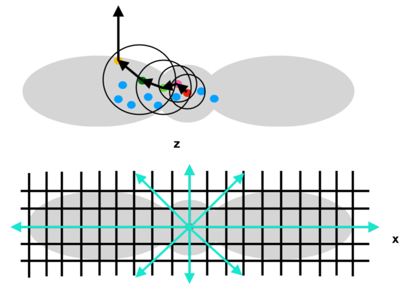
Figure 1: Simplified sketches of the particle-based (top) and grid-based (bottom) approaches for the optical depth calculation. Shown in grey is a neutron star remnant surrounded by a disk. In the particle-based model, each particle has a smoothing length defining the radius of each circle. The latter encloses the particle neighbours. Unlike the grid-based approach, where outgoing radial paths are a priori selected for calculating the optical depth, in the particle-based case the path along which neutrinos move is defined by the density distribution, and therefore it can be non-straight.

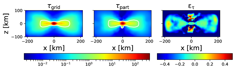
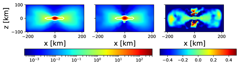
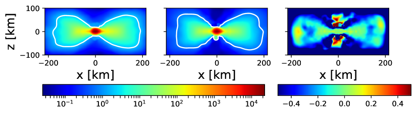
Figure 2: Total optical depth on the x-z plane for electron neutrinos (top), electron anti-neutrinos (middle) and heavy-lepton neutrinos (bottom). For each species we show the map for both a low energy ($\sim 10$ MeV, top) and a high energy ($\sim 100$ MeV, bottom) bin of the spectrum. Moreover, from left to right, we show the maps obtained from the grid-based and particle-based calculations, and a map of the relative difference $\epsilon_{\tau}=\frac{\tau_{\rm{grid}}-\tau_{\rm{part}}}{\tau_{\rm{grid}}}$, respectively.

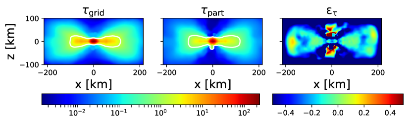
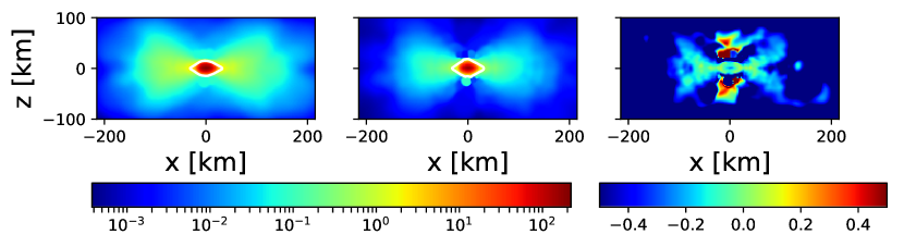
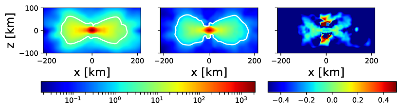
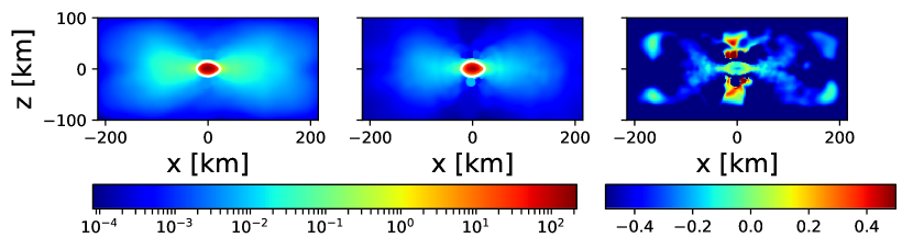
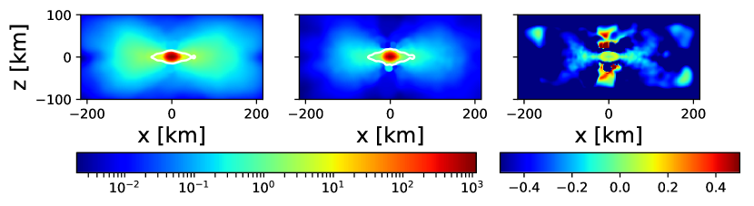
Figure 3: Same as Fig. 2, but for the energy optical depth.

4 Calibration

4.1 Setup

We take three snapshots of binary neutron star merger remnants from the SPH simulations of Rosswog et al. (2017), each one representing a specific case for calibrating our scheme:

case 1) an equal mass binary system of 1.4-1.4 $M_{\odot}$ at $\approx 38$ ms after merger. This is our late-time configuration, when the matter around the remnant has the highest degree of axial symmetry.

case 2) an equal mass binary system of 1.3-1.3 $M_{\odot}$ at $\approx 18$ ms after merger. In this way we include equal mass configurations at earlier post-merger times, when the matter distribution is not fully axially symmetric.

case 3) an unequal mass binary system of 1.2-1.3 $M_{\odot}$ at $\approx 18$ ms after merger. We consider this case as representative of unequal mass binaries at early times, with the lowest degree of axial symmetry.

We use cases 2) and 3) to test the assumption of axial symmetry entering Eq. 5. Table 1 summarises the properties of each binary configuration.

Table 1: Summary of the binary properties for each case examined. We report the masses $m_{1}$ and $m_{2}$ of each star in the binary, the mass ratio $q=m_{2}/m_{1}$ and the time after merger.

Case	$m_{1}(M_{\odot})$	$m_{2}(M_{\odot})$	$q$	time after merger (ms)
1	1.4	1.4	1.00	$\approx$ 38
2	1.3	1.3	1.00	$\approx$ 18
3	1.3	1.2	0.92	$\approx$ 18

Since the snapshots are taken from simulations that use a grey leakage scheme (Rosswog & Liebendörfer, 2003), we first map the SPH properties on a 3D grid and let the radiation field equilibrate with M1 for 3 ms without changing either the electron fraction or the temperature. Afterwards, we let the electron fraction evolve for 10 ms with M1 to remove grey leakage effects. We do not consider the temperature evolution in M1 since we do not see important differences between the corresponding evolved and non-evolved profiles. The evolution with M1 allows to make a more consistent comparison between neutrino approaches for our parameter calibration. Figs. 4-5 show density, temperature and electron fraction in the equatorial plane and on the plane orthogonal to it after the 10 ms of evolution, and for each case. In order to considerably reduce computational costs when running the Monte Carlo code Sedonu we map density, temperature and the evolved electron fraction from M1 onto a 2D, axially symmetric grid, and run the transport over the obtained profiles. At last, we map the evolved M1 data back to the SPH particles by tri-linear interpolation to run the ASL scheme.

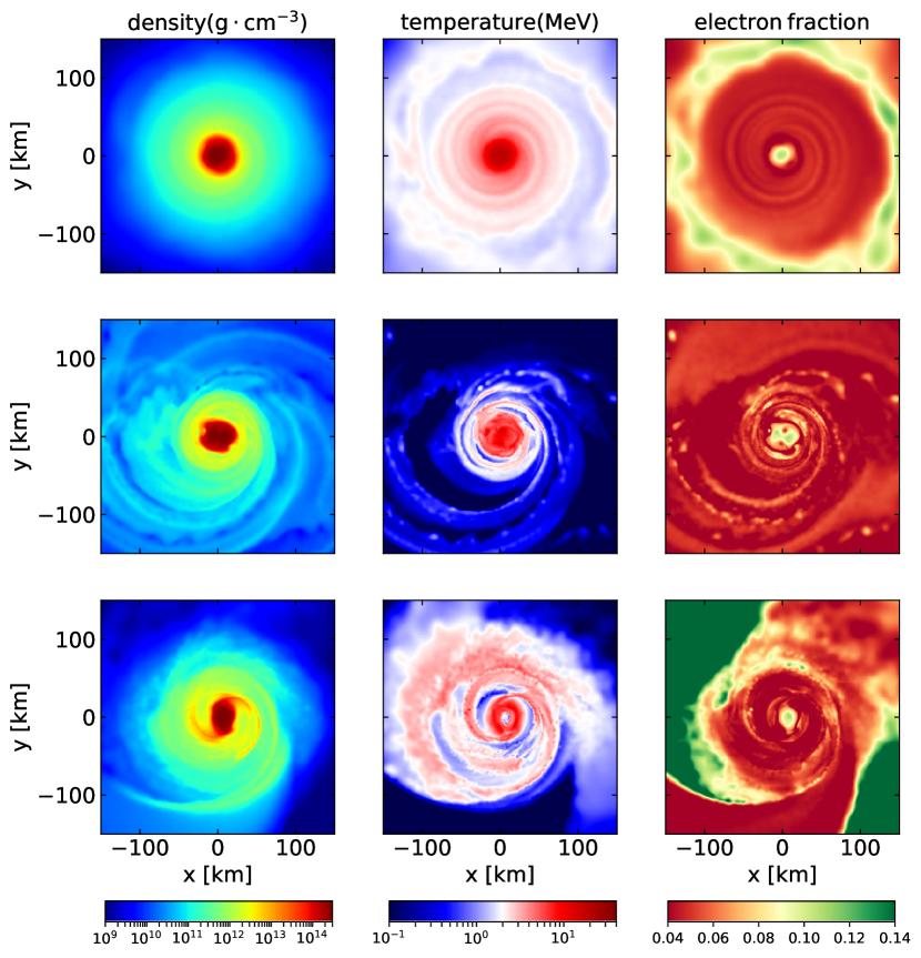
Figure 4: Density (left column), temperature (middle column), and electron fraction (right column) maps on the equatorial plane at equilibrium, for a 1.4-1.4 $M_{\odot}$ binary neutron star merger at $\approx 38$ ms after merger (top row), a 1.3-1.3 $M_{\odot}$ binary neutron star merger at $\approx 18$ ms after merger (middle row), and a 1.2-1.3 $M_{\odot}$ binary neutron star merger at $\approx 18$ ms after merger (bottom row). From top to bottom the degree of axial symmetry of the remnant decreases. Snapshots are taken from the dynamical simulations of Rosswog et al. (2017).

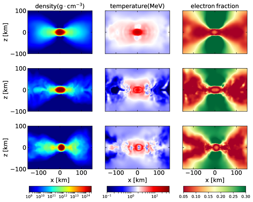
Figure 5: Same as in Fig. 4, but on the plane orthogonal to the equatorial one.

4.2 Strategy

As a first step we identify physical quantities that are directly impacted by each ASL parameter:

1) the total luminosities and mean energies, primarily affected by $\alpha_{\nu,\rm{blk}}$ and $\tau_{\rm{cut}}$.

2) the neutrino flux at different polar angles that an observer located far outside the neutrino surfaces would measure. In this respect, we focus on the trend of the flux with the polar angle for constraining the parameter $p$ in Eq. 5.

Given that the Monte Carlo approach converges (in the limit of infinite particle numbers) to an exact solution of the transport equation, the best strategy for our parameter calibration would be to extract both quantities 1) and 2) from Sedonu and compare with the ASL scheme. However, the assumption of axial symmetry may not be fully appropriate in all cases, especially shortly after merger. We then first test the assumption of azimuthal symmetry by running the M1 transport on both 2D and 3D grid setups, and compare the neutrino emission maps for each species. For those snapshots where the impact on the emission is large in at least one of the species, we decide to consider M1 in 3D for the calibration. However, given the limitations of M1 in accurately modelling the distribution of the neutrino flux at different polar angles (Foucart et al., 2018), we make use of M1 purely for calibrating $\alpha_{\nu,\rm{blk}}$ and $\tau_{\rm{cut}}$, while we keep Sedonu to calibrate the heating parameter $p$. As we shall see, the 2D assumption does not impact the trend of the flux at different polar angles, but only its local values. On the other hand, if the 2D assumption does not affect the emission of any neutrino species sensitively, the calibration of $\alpha_{\nu,\rm{blk}}$, $\tau_{\rm{cut}}$ and of the heating parameter $p$ is performed entirely with Sedonu.
The parameter space we explore is given by $\alpha_{\nu,\rm{blk}}\in[0.35,0.45,0.55,0.65,0.75,0.85]$, $\tau_{\rm{cut}}\in[5,10,15,20]$, and $p\in[2,4,6,8,10,12]$. When calibrating, we assume $\alpha_{\rm{blk}}\equiv\alpha_{\nu_{e},\rm{blk}}=\alpha_{\bar{\nu}_{e},\rm{blk}}$, and $\alpha_{\nu_{x},\rm{blk}}=0$, similarly to Perego et al. (2016). We will discuss the accuracy of the assumption $\alpha_{\nu_{e},\rm{blk}}=\alpha_{\bar{\nu}_{e},\rm{blk}}$ in Sec. 5.2. Given that heavy-lepton neutrinos do not contribute to the heating either, we decide to neglect this species entirely when calibrating, and just focus on the other two species. We will anyway report all values of luminosities and mean energies for completeness (see Table 2).
During the calibration process, when exploring luminosities and mean energies, we first compute:

$$\epsilon_{L} = \epsilon_{L_{\nu_{e}}}+\epsilon_{L_{\bar{\nu}_{e}}},$$ (12)

$$\epsilon_{\langle E\rangle} = \epsilon_{\langle E_{\nu_{e}}\rangle}+\epsilon_{\langle E_{\bar{\nu}_{e}}\rangle},$$ (13)

where

$$\epsilon_{L_{i}}=\frac{|L_{i,\rm{ref}}-L_{i,\rm{ASL}}|}{L_{i,\rm{ref}}}$$ (14)

and

$$\epsilon_{\langle E_{i}\rangle}=\frac{|\langle E_{i,\rm{ref}}\rangle-\langle E_{i,\rm{ASL}}\rangle|}{\langle E_{i,\rm{ref}}\rangle},$$ (15)

$i$ labeling neutrinos of species $i\in[\nu_{e},\bar{\nu}_{e}]$, while $L_{i,\rm{ref}}$ and $\langle E_{i,\rm{ref}}\rangle$ are the luminosity and mean energy of species $i$ from the reference solution (either Sedonu or M1). We compare $\epsilon_{L}$ and $\epsilon_{\langle E\rangle}$ and eventually consider the error among the two more sensitive to a variation of the parameters. We look for regions in the parameter space where this error is minimal for a first pre-selection, and subsequently explore $\epsilon_{L_{i}}$ and $\epsilon_{\langle E_{i}\rangle}$ individually for a more detailed analysis.
When calibrating $p$ with Sedonu we assume an analytical form of the neutrino fluxes as function of the polar angle in the ASL scheme. In particular, the flux of neutrinos of species $i$ leaving the source at some distance $R$ is:

$$\textbf{F}_{i}=\frac{1}{R^{2}}\frac{dL_{i}}{d\Omega}\textbf{n},$$ (16)

n being the unit vector orthogonal to the surface $dS=R^{2}d\Omega$, and $d\Omega=d\mathrm{cos}(\theta)d\phi=d\mu d\phi$ being the solid angle of polar angle $\theta$ and azimuthal angle $\phi$. For axial symmetry with $d\Omega=2\pi d\mu$ we have:

$$\textbf{F}_{i}=\frac{1}{2\pi R^{2}}\Big{(}\frac{dL_{i}}{d\mu}\Big{)}\textbf{n}.$$ (17)

Given the analytical angular term in Eq. 5, we assume that:

$$\frac{dL_{i}}{d\Omega}=\frac{1}{4\pi}\frac{(1+p)(1+\beta_{i}\cos^{p}(\theta))}{1+p+\beta_{i}}L_{i}$$ (18)

and

$$\frac{dL_{i}}{d\mu}=\frac{1}{2}\frac{(1+p)(1+\beta_{i}\cos^{p}(\theta))}{1+p+\beta_{i}}L_{i}\,.$$ (19)

We caution the reader that Eq. 19 is purely to understand which value of $p$ best reproduces the trend of the flux as function of the polar angle from Sedonu. We do not attempt to estimate the magnitude of the flux at each polar angle via Eq. 19 because it is not possible to extract this information with a leakage scheme.

We summarise the values of luminosities and mean energies for the three cases described in Sec. 4.1 in Table 2. We include the 2D values from Sedonu, the 2D and 3D values from M1, and the values from the ASL with the corresponding best parameter set when assuming $\alpha_{\rm{blk}}\equiv\alpha_{\nu_{e},\rm{blk}}=\alpha_{\bar{\nu}_{e},\rm{blk}}$.

Table 2: Summary of the values of luminosities and mean energies for each species from Sedonu (2nd column), M1 in 2D (3rd colum), M1 in 3D (4th column) and the ASL (5th column), for each of the three cases (1st column) examined. For the ASL, we also specify the best parameter set resulting from the calibration (6th column) when assuming $\alpha_{\rm{blk}}\equiv\alpha_{\nu_{e},\rm{blk}}=\alpha_{\bar{\nu}_{e},\rm{blk}}$. The reported numbers from Sedonu are accurate in spite of the Monte Carlo noise, which is estimated to be a thousand times smaller.

Case	Sedonu (2D)	M1(2D)	M1(3D)	ASL	[$\alpha_{\rm{blk}}$,$\tau_{\rm{cut}}$,$p$]
1	$L_{\nu_{e}}^{1}=7.50\cdot 10^{51}\rm{erg\>s^{-1}}$	$L_{\nu_{e}}^{1}=7.73\cdot 10^{51}\rm{erg\>s^{-1}}$	$L_{\nu_{e}}^{1}=7.46\cdot 10^{51}\>\rm{erg\>s^{-1}}$	$L_{\nu_{e}}^{1}=6.81\cdot 10^{51}\>\rm{erg\>s^{-1}}$
	$L_{\bar{\nu}_{e}}^{1}=1.50\cdot 10^{52}\>\rm{erg\>s^{-1}}$	$L_{\bar{\nu}_{e}}^{1}=1.63\cdot 10^{52}\>\rm{erg\>s^{-1}}$	$L_{\bar{\nu}_{e}}^{1}=1.75\cdot 10^{52}\>\rm{erg\>s^{-1}}$	$L_{\bar{\nu}_{e}}^{1}=1.71\cdot 10^{52}\>\rm{erg\>s^{-1}}$
	$L_{\nu_{x}}^{1}=2.14\cdot 10^{52}\>\rm{erg\>s^{-1}}$	$L_{\nu_{x}}^{1}=2.91\cdot 10^{52}\>\rm{erg\>s^{-1}}$	$L_{\nu_{x}}^{1}=2.73\cdot 10^{52}\>\rm{erg\>s^{-1}}$	$L_{\nu_{x}}^{1}=2.97\cdot 10^{52}\>\rm{erg\>s^{-1}}$	[0.45,10,2]
	$\langle{}E_{\nu_{e}}\rangle{}=9.24\>\rm{MeV}$	$\langle{}E_{\nu_{e}}\rangle{}=9.37\>\rm{MeV}$	$\langle{}E_{\nu_{e}}\rangle{}=9.38\>\rm{MeV}$	$\langle{}E_{\nu_{e}}\rangle{}=8.70\>\rm{MeV}$
	$\langle{}E_{\bar{\nu}_{e}}\rangle{}=13.05\>\rm{MeV}$	$\langle{}E_{\bar{\nu}_{e}}\rangle{}=13.00\>\rm{MeV}$	$\langle{}E_{\bar{\nu}_{e}}\rangle{}=13.10\>\rm{MeV}$	$\langle{}E_{\bar{\nu}_{e}}\rangle{}=12.88\>\rm{MeV}$
	$\langle{}E_{\nu_{x}}\rangle{}=13.87\>\rm{MeV}$	$\langle{}E_{\nu_{x}}\rangle{}=15.27\>\rm{MeV}$	$\langle{}E_{\nu_{x}}\rangle{}=15.28\>\rm{MeV}$	$\langle{}E_{\nu_{x}}\rangle{}=13.63\>\rm{MeV}$
2	$L_{\nu_{e}}^{1}=8.85\cdot 10^{51}\>\rm{erg\>s^{-1}}$	$L_{\nu_{e}}^{1}=9.03\cdot 10^{51}\>\rm{erg\>s^{-1}}$	$L_{\nu_{e}}^{1}=7.29\cdot 10^{51}\>\rm{erg\>s^{-1}}$	$L_{\nu_{e}}^{1}=5.65\cdot 10^{51}\>\rm{erg\>s^{-1}}$
	$L_{\bar{\nu}_{e}}^{1}=8.64\cdot 10^{51}\>\rm{erg\>s^{-1}}$	$L_{\bar{\nu}_{e}}^{1}=9.39\cdot 10^{51}\>\rm{erg\>s^{-1}}$	$L_{\bar{\nu}_{e}}^{1}=1.90\cdot 10^{52}\>\rm{erg\>s^{-1}}$	$L_{\bar{\nu}_{e}}^{1}=1.80\cdot 10^{52}\>\rm{erg\>s^{-1}}$
	$L_{\nu_{x}}^{1}=2.00\cdot 10^{52}\>\rm{erg\>s^{-1}}$	$L_{\nu_{x}}^{1}=2.57\cdot 10^{52}\>\rm{erg\>s^{-1}}$	$L_{\nu_{x}}^{1}=2.90\cdot 10^{52}\>\rm{erg\>s^{-1}}$	$L_{\nu_{x}}^{1}=4.10\cdot 10^{52}\>\rm{erg\>s^{-1}}$	[0.65,10,2]
	$\langle{}E_{\nu_{e}}\rangle{}=10.65\>\rm{MeV}$	$\langle{}E_{\nu_{e}}\rangle{}=10.89\>\rm{MeV}$	$\langle{}E_{\nu_{e}}\rangle{}=11.11\>\rm{MeV}$	$\langle{}E_{\nu_{e}}\rangle{}=10.43\>\rm{MeV}$
	$\langle{}E_{\bar{\nu}_{e}}\rangle{}=15.74\>\rm{MeV}$	$\langle{}E_{\bar{\nu}_{e}}\rangle{}=15.69\>\rm{MeV}$	$\langle{}E_{\bar{\nu}_{e}}\rangle{}=16.23\>\rm{MeV}$	$\langle{}E_{\bar{\nu}_{e}}\rangle{}=16.61\>\rm{MeV}$
	$\langle{}E_{\nu_{x}}\rangle{}=14.01\>\rm{MeV}$	$\langle{}E_{\nu_{x}}\rangle{}=14.98\>\rm{MeV}$	$\langle{}E_{\nu_{x}}\rangle{}=16.05\>\rm{MeV}$	$\langle{}E_{\nu_{x}}\rangle{}=15.54\>\rm{MeV}$
3	$L_{\nu_{e}}^{1}=2.04\cdot 10^{52}\>\rm{erg\>s^{-1}}$	$L_{\nu_{e}}^{1}=9.36\cdot 10^{51}\>\rm{erg\>s^{-1}}$	$L_{\nu_{e}}^{1}=6.27\cdot 10^{51}\>\rm{erg\>s^{-1}}$	$L_{\nu_{e}}^{1}=3.01\cdot 10^{51}\>\rm{erg\>s^{-1}}$
	$L_{\bar{\nu}_{e}}^{1}=2.78\cdot 10^{51}\>\rm{erg\>s^{-1}}$	$L_{\bar{\nu}_{e}}^{1}=2.98\cdot 10^{51}\>\rm{erg\>s^{-1}}$	$L_{\bar{\nu}_{e}}^{1}=2.24\cdot 10^{52}\>\rm{erg\>s^{-1}}$	$L_{\bar{\nu}_{e}}^{1}=2.86\cdot 10^{52}\>\rm{erg\>s^{-1}}$
	$L_{\nu_{x}}^{1}=1.24\cdot 10^{52}\>\rm{erg\>s^{-1}}$	$L_{\nu_{x}}^{1}=1.45\cdot 10^{52}\>\rm{erg\>s^{-1}}$	$L_{\nu_{x}}^{1}=2.40\cdot 10^{52}\>\rm{erg\>s^{-1}}$	$L_{\nu_{x}}^{1}=3.55\cdot 10^{52}\>\rm{erg\>s^{-1}}$	[0.75,10,2]
	$\langle{}E_{\nu_{e}}\rangle{}=6.88\>\rm{MeV}$	$\langle{}E_{\nu_{e}}\rangle{}=10.60\>\rm{MeV}$	$\langle{}E_{\nu_{e}}\rangle{}=9.90\>\rm{MeV}$	$\langle{}E_{\nu_{e}}\rangle{}=9.61\>\rm{MeV}$
	$\langle{}E_{\bar{\nu}_{e}}\rangle{}=13.17\>\rm{MeV}$	$\langle{}E_{\bar{\nu}_{e}}\rangle{}=14.10\>\rm{MeV}$	$\langle{}E_{\bar{\nu}_{e}}\rangle{}=15.61\>\rm{MeV}$	$\langle{}E_{\bar{\nu}_{e}}\rangle{}=18.85\>\rm{MeV}$
	$\langle{}E_{\nu_{x}}\rangle{}=11.42\>\rm{MeV}$	$\langle{}E_{\nu_{x}}\rangle{}=12.39\>\rm{MeV}$	$\langle{}E_{\nu_{x}}\rangle{}=15.56\>\rm{MeV}$	$\langle{}E_{\nu_{x}}\rangle{}=16.62\>\rm{MeV}$

5 Results

In Sec. 5.1, we describe the calibration of each ASL parameter based on a separate analysis for each snapshot. Afterwards, we combine the results in Sec. 5.2 and discuss the performance of using the same blocking parameter for electron neutrinos and anti-neutrinos.

5.1 Parameter constraints

5.1.1 Blocking

From Table 2 we can see that by comparing the 2D and 3D luminosities of electron neutrinos and anti-neutrinos from M1 the impact of the 2D averaging is only of the order of $\lesssim 7\%$ for both species in case 1). This suggests the usage of Sedonu for the comparison with the ASL scheme. On the other hand, for cases 2) and 3) the 2D averaging implies a reduction in the electron anti-neutrino luminosity by about a factor of 2 and 10 respectively. We examine the effect of the 2D averaging on the emission maps for each species, and we indeed notice that the 2D assumption affects the neutrino species to a different extent, depending on the respective location of the bulk of the emission. We therefore decide to take the 3D M1 values of luminosities and mean energies as reference for calibrating $\alpha_{\rm{blk}}$ and $\tau_{\rm{cut}}$ in cases 2) and 3). We also notice that the heavy-lepton neutrino luminosity from M1 in 3D and from the ASL is systematically larger by a factor of a few than the one from Sedonu in all snapshots. This is different from the results of Foucart et al. (2020). However, the fact that only heavy-lepton neutrinos show large deviations with respect to a Monte Carlo approach is an indication that the cause might be associated to some ingredient in the particular transport approach adopted, and for which heavy-leptons are more affected than the other species. Regarding the ASL, a likely explanation is the treatment of the emission rate, which is calculated as smooth interpolation between production and diffusion rates as shown in Eq. 2. The diffusion rate depends on the diffusion timescale, which is estimated via a random-walk argument. As pointed out in Ardevol-Pulpillo et al. (2019), this derivation leads to a steeper decrease of the diffusion timescale with radius. Combined with the fact that most of the neutrinos escape around the rather small region of the neutrino surface, a lower diffusion timescale in this region can boost the emission up to more than a factor of 2, depending on the species. For our binary neutron star configurations, this is particularly true for heavy-lepton neutrinos because their sources of production are just pair processes and bremsstrahlung, which are both extremely temperature-dependent. Combined with the fact that heavy-lepton neutrinos decouple at inner and still rather hot regions with respect to the other two species, it is likely that their emission is more affected by the treatment of the diffusion.
Fig. 6 shows line plots of $\epsilon_{L}$ and $\epsilon_{\langle E\rangle}$ as a function of $\alpha_{\rm{blk}}$, for different values of $p$ and $\tau_{\rm{cut}}$. Lines of the same color are for fixed $p$, while lines of the same type are for fixed $\tau_{\rm{cut}}$. We neglect the cases with $\tau_{\rm{cut}}=5$ and $p=12$ to reduce the amount of data to show, but the results do not change. From the top to the bottom row we show the cases from 1) to 3) respectively. Generally, we see that neither $\epsilon_{L}$ nor $\epsilon_{\langle E\rangle}$ is largely affected by varying $p$ for a given $\alpha_{\rm{blk}}$ and $\tau_{\rm{cut}}$. The mild dependence can be explained by the fact that $p$ defines the distribution of the heating rather than its intensity. However, because the neutrino absorption is typically more pronounced for electron neutrinos than for anti-neutrinos, we should expect a somewhat larger dependence of $\epsilon_{L}$ on $p$ for the former species. Nevertheless, since we are evaluating the species-summed $\epsilon_{L}$, even in case there is such dependence from the electron neutrinos, this must be associated to a rather small $\epsilon_{L_{\nu_{e}}}$ (see later Fig. 7), and it is thus not appreciable. On the other hand, the blocking parameter $\alpha_{\rm{blk}}$ has a major impact on $\epsilon_{L}$. This comes directly from the $r_{\nu}\rightarrow(1-\alpha_{\rm{blk}})r_{\nu}$ correction to the emission rate $r_{\nu}$ when accounting for blocking, see Eq. 2. This is different from the impact on $\epsilon_{E}$, which is basically negligible. The reason is the fact that $\langle E_{i}\rangle$ is computed from the ratio between the luminosity $L_{i}$ [erg/s] and the total number of emitted neutrinos of species $i$ per unit time, both affected by blocking for the case of electron neutrinos and anti-neutrinos. At last, a noticeable dependence to $\tau_{\rm{cut}}$ can be seen from $\epsilon_{\langle E\rangle}$, as a consequence of the fact that $\tau_{\rm{cut}}$ impacts the neutrino spectrum at the decoupling region, and therefore the mean energies of the species. We find that $\epsilon_{\langle E\rangle}$ has a maximum value of $\sim 18\%$ and $\sim 12\%$ at $\tau_{\rm{cut}}=5$ for cases 1) and 2) respectively. Case 3) shows larger values, but limited to $<30\%$. On the other hand, $\epsilon_{L}$ varies from $\sim 10\%$ to more than $100\%$ for cases 1) and 2), while case 3) shows values $\epsilon_{L}\gtrsim 0.75$. The large $\epsilon_{L}$ for any parameter combination for the latter case is a consequence of the $\alpha_{\rm{blk}}=\alpha_{\nu_{e},\rm{blk}}=\alpha_{\bar{\nu}_{e},\rm{blk}}$ assumption, which makes it cumbersome to always well catch the luminosities of both electron neutrinos and anti-neutrinos (see also Fig. 7 and next paragraph). Since $\epsilon_{L}$ is more sensitive than $\epsilon_{\langle E\rangle}$ to a change in $\alpha_{\rm{blk}}$, we just look at $\epsilon_{L}$ for a first parameter pre-selection. In particular, we find a minimum $\epsilon_{L}$ around $\alpha_{\rm{blk}}=0.45$ for case 1), $\alpha_{\rm{blk}}=0.65$ for case 2), and $\alpha_{\rm{blk}}=0.75$ for case 3).

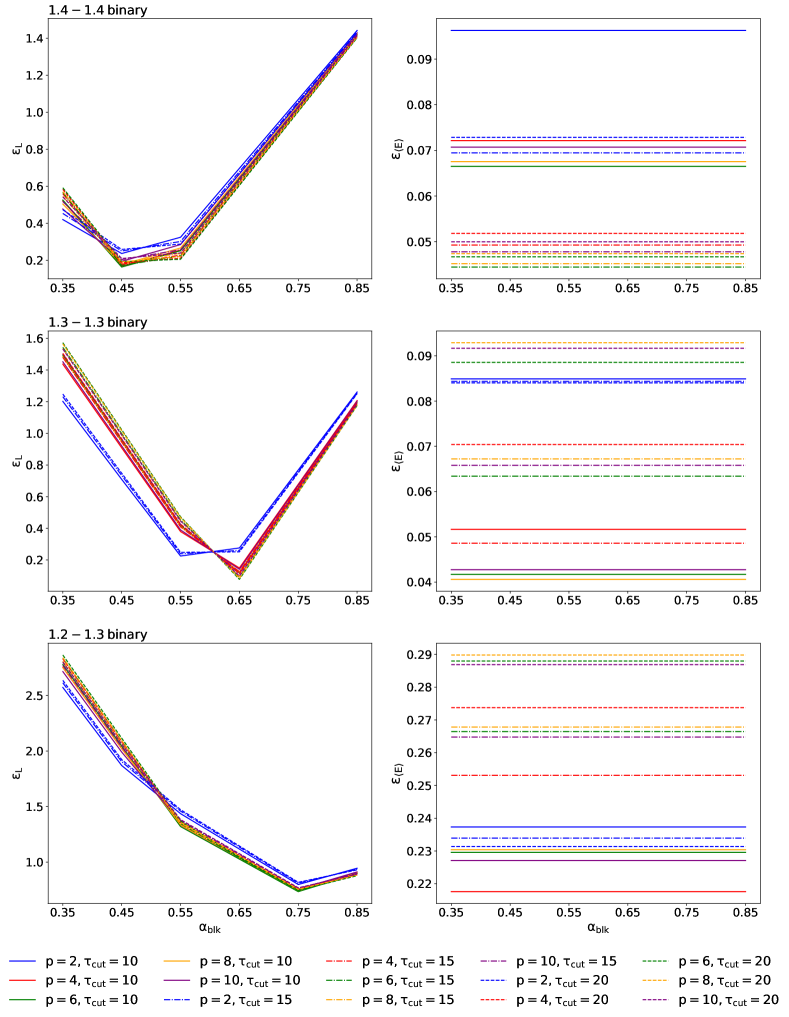
Figure 6: Relative difference on the luminosity $\epsilon_{L}$ (left panels) and the mean neutrino energy $\epsilon_{\langle E\rangle}$ (right panels) as a function of $\alpha_{\rm{blk}}$ and for different values of $p$ and $\tau_{\rm{cut}}$, calculated by comparing the results from the ASL with the reference solution. From top to bottom, we show cases from 1) to 3). We use Sedonu as reference solution for case 1), and M1 for cases 2) and 3). Lines of the same color are for fixed $p$, while lines of the same type are for fixed $\tau_{\rm{cut}}$. We neglect the cases with $\tau_{\rm{cut}}=5$ to reduce the amount of data to show. The parameter $\alpha_{\rm{blk}}$ has a large impact on $\epsilon_{L}$, but not on $\epsilon_{\langle E\rangle}$. The thermalization parameter $\tau_{\rm{cut}}$ has some effect on $\epsilon_{\langle E\rangle}$, while $p$ mildly impacts both $\epsilon_{L}$ and $\epsilon_{\langle E\rangle}$.

5.1.2 Thermalization

We set $\alpha_{\rm{blk}}$ to the above values, and look at both $\epsilon_{L_{i}}$ and $\epsilon_{\langle E_{i}\rangle}$ for each species $i\in[\nu_{e},\bar{\nu}_{e}]$ in Fig. 7. The first two rows correspond to the results for case 1), the third and fourth row to the results for case 2), and the last two rows for case 3). We show both results for electron neutrinos (left column) and for electron anti-neutrinos (right column). As anticipated before, $\epsilon_{L_{\nu_{e}}}$ shows the largest dependence on $p$ for a given $\tau_{\rm{cut}}$. We find that for electron neutrinos $\epsilon_{L_{\nu_{e}}}\lesssim 12\%$, $\epsilon_{L_{\nu_{e}}}\lesssim 23\%$ and $\epsilon_{L_{\nu_{e}}}\lesssim 52\%$ for cases 1), 2) and 3) respectively. If we look at electron anti-neutrinos we have $\epsilon_{L_{\bar{\nu}_{e}}}$ up to $\sim 20\%$, $\epsilon_{L_{\bar{\nu}_{e}}}\lesssim 8\%$ and $\epsilon_{L_{\bar{\nu}_{e}}}\lesssim 31\%$ respectively. On the other hand, $\epsilon_{\langle E_{i}\rangle}\lesssim 12\%$ for each species $i$ in cases 1) and 2), while case 3) shows $\epsilon_{\langle E_{\bar{\nu}_{e}}\rangle}\lesssim 23\%$. While the overall limited values in both $\epsilon_{L_{i}}$ and $\epsilon_{\langle E_{i}\rangle}$ suggest that any value of $\tau_{\rm{cut}}\in[5,10,15,20]$ seems good enough to describe the thermalization for both cases 1) and 2), in case 3) only either $\tau_{\rm{cut}}=5$ or $\tau_{\rm{cut}}=10$ is able to keep $\epsilon_{L_{\bar{\nu}_{e}}}<30\%$, in spite of the large $\epsilon_{L_{\nu_{e}}}\gtrsim 52\%$. We therefore always take $\tau_{\rm{cut}}=10$ as reference for the ASL luminosities and mean energies shown in Table 2.
We notice that the electron neutrino and anti-neutrino mean energies are systematically higher for cases 2) and 3) in both the M1 and the ASL by up to $\sim 1-3$ MeV with respect to case 1). We provide an explanation by calculating the average temperatures at which both neutrino species are emitted by means of equation 9 of Rosswog & Liebendörfer (2003). Table 3 shows the results we find. The average temperatures are higher by $\gtrsim 1$ MeV with respect to case 1), implying that most of the emission for both electron neutrinos and anti-neutrinos comes from hotter regions. Since neutrinos thermalize with matter before free-streaming, the mean neutrino energy is higher if temperatures are higher. The presence of hotter regions is also confirmed by the fact that the maximum temperature seen for case 1) is $\sim 25$ MeV, while for case 2) reaches $\sim 40$ MeV and for case 3) $\sim 32$ MeV. However, the higher electron anti-neutrino mean energy in case 3) is also a consequence of the rather large $\epsilon_{\bar{\nu}_{e}}$ (Fig. 7, right panel on the sixth row).

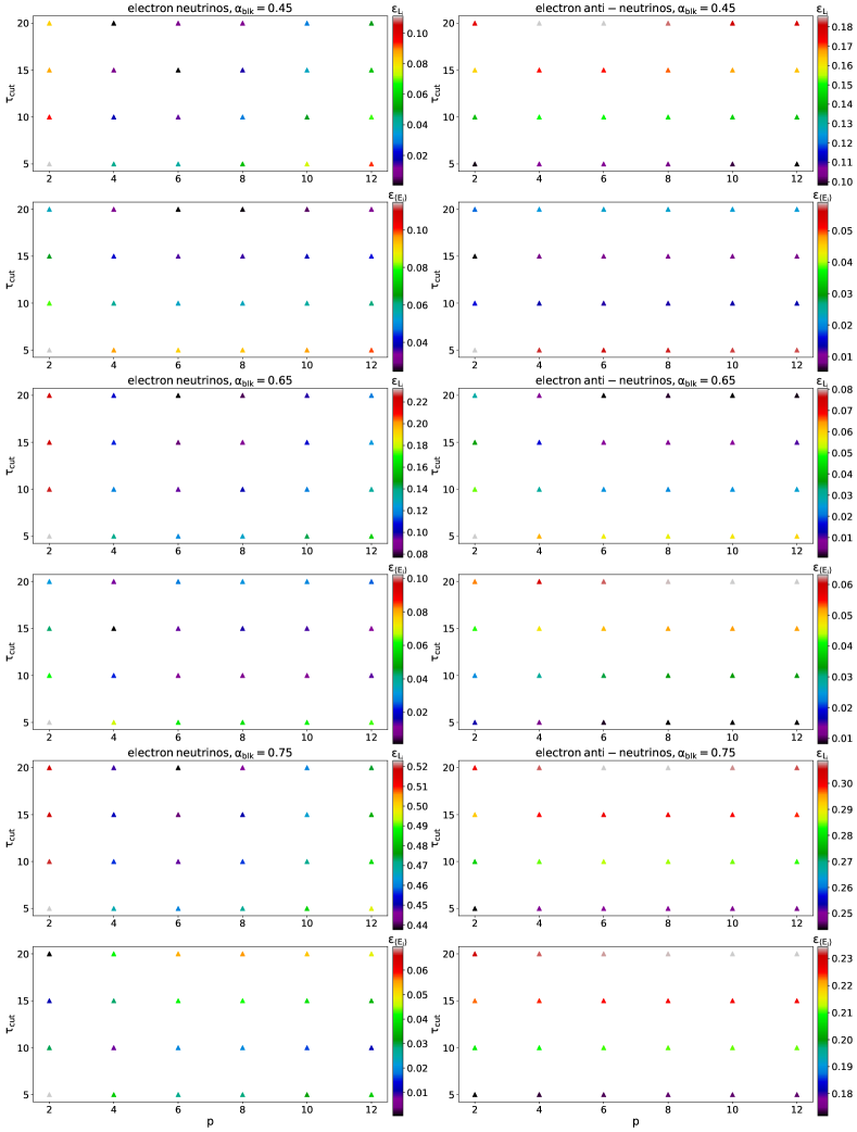
Figure 7: Relative difference on the luminosity $\epsilon_{L_{i}}$ and the mean energy $\epsilon_{\langle E_{i}\rangle}$ for $i=\nu_{e}$ (left panels) and $i=\bar{\nu}_{e}$ (right panels), and for case 1) (first and second row), case 2) (third and fourth row), and case 3) (fifth and sixth row), calculated by comparing the results from the ASL with the reference solution. We use Sedonu as reference solution for case 1), and M1 for cases 2) and 3). While $\epsilon_{\langle E_{i}\rangle}$ is always limited to $\lesssim 23\%$ at the most for electron anti-neutrinos in case 3), the assumption of a single blocking parameter for both electron neutrinos and anti-neutrinos leads to inaccurate recoveries of the neutrino luminosities in some cases, with $\epsilon_{L_{\nu_{e}}}$ up to $52\%$.

5.1.3 Heating

To constrain the heating parameter $p$, we show in the first three rows of Fig. 8 $dL_{i}/d\mu$ as a function of $\theta$ for all cases examined, and for $i=\nu_{e}$ (left panels), $i=\bar{\nu}_{e}$ (right panels). The curve from M1 is obtained by taking an average of $dL_{i}/d\mu$ over different azimuthal angles $\phi$ of the domain for each polar angle $\theta$, while the ASL curve is obtained by means of Eq. 19, with the best blocking parameter, a reference value of $\tau_{\rm{cut}}=10$ , and the best $p$ from the direct comparison between the polar angle profiles of the luminosities. Unlike case 1), we only show the 2D result from Sedonu and the ASL curve of $dL_{\bar{\nu}_{e}}/d\mu$ for cases 2) and 3) because of the impact of the 2D assumption on the electron anti-neutrino emission. We see that $p=2$ nicely fits trends from Sedonu for both electron neutrinos and anti-neutrinos and in all cases. We can also see that M1 overestimates the flux close to the polar axis for both electron neutrinos and anti-neutrinos in cases 1) and 2), with a maximum disagreement with respect to the result from Sedonu by a factor of $\lesssim 2$ at the pole in case 1). This is in accordance with the previous findings of Foucart et al. (2018, 2020), and it is the result of the approximations introduced by the analytical closure. It is also important to notice that our new estimate of the parameter $p=2$ is lower than the one we found in Gizzi et al. (2019), where we estimated $p=8$. The reason is the fact that there we chose M1 as source for comparison. As just said, the approximations introduced by the analytical closure inevitably leads to a steeper decrease of the neutrino fluxes with the polar angle, consequently suggesting a larger value of $p$ than the one found here. We justify our decision of using the 2D data from Sedonu of electron anti-neutrinos in cases 2) and 3) for the calibration of $p=2$ by noticing that the 2D assumption does not impact the trend of $dL_{\bar{\nu}_{e}}/d\mu$ in M1 (see purple curve in the last row of Fig. 8). The last row shows also the quantity $dL_{\bar{\nu}_{e}}/d\mu$ as function of the polar angle $\theta$ for different azimuthal angles $\phi$, obtained with M1 in 3D (green dots). We can clearly see that the variation with $\phi$ is limited, particularly at angles $\theta\lesssim\pi/3\approx 1.05$ where the bulk of neutrino-driven winds is located. This justifies the assumption of axially symmetric fluxes entering Eq. 5.

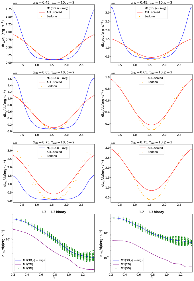
Figure 8: $dL_{i}/d\mu$ as a function of $\theta$. From the first to the third row we show the results for cases from 1) to 3) respectively, for $i=\nu_{e}$ (left) and $i=\bar{\nu}_{e}$ (right). Dots represent the exact solution from Sedonu. The blue curve describes the trend of $dL_{i}/d\mu$ obtained with M1 when performing an azimuthal average over different $\phi$ at each $\theta$, while the red curve describes the one from the ASL, scaled by some constant, and obtained via Eq. 19 with the best parameter set of each case. We only show the trends from Sedonu and ASL for anti-neutrinos in cases 2) and 3). The trend from Sedonu is overall well described by a $\rm{cos}^{2}(\theta)$ for both species and in all cases. M1 tends to overestimate the flux close to the polar axis for both electron neutrinos and anti-neutrinos, as a consequence of the approximations introduced by the analytical closure. The last row shows $dL_{\bar{\nu}_{e}}/d\mu$ as a function of $\theta$ for case 2) (left), and case 3) (right). The 2D assumption does not affect the trend of $dL_{\bar{\nu}_{e}}/d\mu$. Moreover, for a given $\theta$ we see a limited variation of $dL_{\bar{\nu}_{e}}/d\mu$ with $\phi$ at polar angles relevant for neutrino-driven winds ($\theta\lesssim\pi/3$).

Table 3: Average densities (2nd and 3rd columns), temperatures (4th and 5th columns) and electron fractions (6th and 7th columns) at which electron neutrinos and anti-neutrinos are emitted, and difference between average electron anti-neutrino and electron neutrino degeneracy parameters (8th column), for each of the three cases examined (1st column). The computation of the averages follows equation 9 of Rosswog & Liebendörfer (2003). For the computation of the neutrino chemical potentials entering the degeneracy parameters, we assume weak equilibrium.

Case	$\langle\rho\rangle_{\nu_{e}}$[$\rm{10^{13}\>g\cdot cm^{-3}}$]	$\langle\rho\rangle_{\bar{\nu}_{e}}$[$\rm{10^{13}\>g\cdot cm^{-3}}$]	$\langle T\rangle_{\nu_{e}}$[MeV]	$\langle T\rangle_{\bar{\nu}_{e}}$[MeV]	$\langle Y_{e}\rangle_{\nu_{e}}$	$\langle Y_{e}\rangle_{\bar{\nu}_{e}}$	$\langle\eta\rangle_{\bar{\nu}_{e}}-\langle\eta\rangle_{\nu_{e}}$
1	0.86	1.77	4.37	5.46	0.075	0.070	1.38
2	1.18	1.03	5.51	6.55	0.104	0.091	0.95
3	0.80	0.52	5.16	6.41	0.085	0.073	1.93

5.2 Combination of parameter constraints

Among the three calibrated parameters, both $\tau_{\rm{cut}}$ and $p$ do not show variations by changing the binary configuration. In particular, $\tau_{\rm{cut}}$ is always around a value of 10, and $p=2$. On the other hand, $\alpha_{\rm{blk}}$ is more sensitive than the other parameters when moving from one binary configuration to another. Similar to the results of Perego et al. (2016), the blocking parameter may vary in a range [0.45,0.75], depending on the configuration of the binary and its time after merger. Under the assumption $\alpha_{\rm{blk}}\equiv\alpha_{\nu_{e},\rm{blk}}=\alpha_{\bar{\nu_{e}},\rm{blk}}$, we find larger values of $\alpha_{\rm{blk}}$ for cases 2) and 3) with respect to case 1). Specifically, $\alpha_{\rm{blk}}$ is $\sim 44\%$ and $\sim 66\%$ larger respectively. However, it is important to consider that the values of luminosities and mean energies from M1 that we have taken as reference in cases 2) and 3) might be off by $\sim 20\%$ with respect to an exact solution to the transport (Foucart et al., 2020), implying that our calibrated $\alpha_{\rm{blk}}$ might be slightly affected too.
We find that assuming $\alpha_{\nu_{e},\rm{blk}}=\alpha_{\bar{\nu_{e}},\rm{blk}}$ is not a good choice at early times after merger. In particular, we notice that higher values of $\alpha_{\rm{blk}}$ do not well capture the total luminosity of electron neutrinos (see left panels in the third and fifth row of Fig. 7), pointing to the need for $\alpha_{\nu_{e},\rm{blk}}<\alpha_{\bar{\nu}_{e},\rm{blk}}$. This conclusion is consistent with the fact that electron anti-neutrinos are the most emitted species in merger environments, and therefore likely more affected by blocking effects. Moreover, we find the electron anti-neutrino gas to have on average fewer energy states available to be populated by new emitted neutrinos of the same species. Indeed, by calculating the difference between the average degeneracy parameter of electron neutrinos and anti-neutrinos, we find positive values for all the cases examined (see 8th column of Table 3). In light of this, we optimize the choice of blocking parameter by exploring in Fig 9 $\epsilon_{L_{i}}$ for $i=[\nu_{e},\bar{\nu}_{e}]$ and for the three cases examined in Sec. 4 by assuming $\tau_{\rm{cut}}=10$, $p=2$ and $\alpha_{\nu_{e},\rm{blk}}\neq\alpha_{\bar{\nu_{e}},\rm{blk}}$. We confirm that for each binary the value of the blocking corresponding to the minimum $\epsilon_{L_{i}}$ is lower for $i=\nu_{e}$ than for $i=\bar{\nu}_{e}$. For electron neutrinos, the largest blocking parameter at which $\epsilon_{L_{\nu_{e}}}$ is minimum is found in case 2), with $\alpha_{\nu_{e},\rm{blk}}=0.55$. By looking at Table 3, this is on one side due to the larger average emission temperature (${\langle T\rangle}_{\nu_{e}}=5.51\>\rm{MeV}$), for which the emission rate is enhanced considerably due to the $\sim T^{5}$ dependence for charged-current interactions (Rosswog & Liebendörfer, 2003), and on the other side to the less neutron-rich environment (${\langle Y_{e}\rangle}_{\nu_{e}}=0.104$) that favours electron captures on protons. Both factors contribute in providing more electron neutrinos, and therefore enhancing Pauli blocking effects. For electron anti-neutrinos the largest blocking parameter at which $\epsilon_{L_{\bar{\nu}_{e}}}$ is minimum is found for case 3), with $\alpha_{\bar{\nu}_{e},\rm{blk}}=0.75-0.85$. Again, this is due to both a rather hot (${\langle T\rangle}_{\bar{\nu}_{e}}=6.41\>\rm{MeV}$) and neutron-rich material (${\langle Y_{e}\rangle}_{\nu_{e}}=0.073$) that favours positron captures on neutrons. A value of $\alpha_{\nu_{e},\rm{blk}}=0.45$ provides $\epsilon_{L_{\nu_{e}}}\lesssim 20\%$ for all binaries, and we therefore set it as fiducial for this species. Regarding the anti-neutrinos, the variability of $\epsilon_{L_{\bar{\nu}_{e}}}$ with $\alpha_{\bar{\nu}_{e},\rm{blk}}$ is larger and makes the choice of the best blocking parameter more cumbersome. In particular, equal mass binaries prefer $\alpha_{\bar{\nu}_{e},\rm{blk}}=0.55$ and $\alpha_{\bar{\nu}_{e},\rm{blk}}=0.65$, for cases 1) and 2) respectively, while case 3) prefers $\alpha_{\bar{\nu}_{e},\rm{blk}}>0.65$. We therefore suggest a fiducial value of $\alpha_{\bar{\nu}_{e},\rm{blk}}=0.55$ for equal mass binaries, such that $\epsilon_{L_{\bar{\nu}_{e}}}\lesssim 20\%$, and $\alpha_{\bar{\nu}_{e},\rm{blk}}=0.75$ for unequal mass binaries, such that $\epsilon_{L_{\bar{\nu}_{e}}}<30\%$. However, the unequal mass case might need to be explored in other test cases for a more robust gauging of $\alpha_{\bar{\nu}_{e},\rm{blk}}$. Beside the thermodynamical, compositional and degeneracy properties of the matter described in Table 3 and determining the extent of Pauli blocking, the increasing value of the blocking parameter for both electron neutrinos and anti-neutrino species when moving from case 1) to case 3) is also consistent with the fact that generally less massive and/or unequal mass binaries produce larger disks (Rosswog et al., 2000; Vincent et al., 2020; Bernuzzi et al., 2020). As stated in Sec. 2.3, the blocking parameter takes also into account the reduction of neutrino emission due to inward neutrino fluxes in the semi-transparent regime. The presence of larger disks in less massive and/or unequal mass binaries leads to larger neutrino surfaces, and consequently to an overall larger effect of inward neutrino fluxes, therefore contributing to an increase in the size of blocking.
We conclude by showing in Figs. 10-11 the distribution of the rate of change of the specific matter internal energy $\dot{e}$ (units of $10^{20}\>\rm{erg}\>\rm{g}^{-1}\>\rm{s}^{-1}$) and of the electron fraction $\dot{Y}_{\rm{e}}$ in the winds for case 1) and for the different transport approaches, assuming $\alpha_{\nu_{e},\rm{blk}}=0.45,\alpha_{\bar{\nu}_{e},\rm{blk}}=0.55,\tau_{\rm{cut}}=10,p=2$. The upper plots are 3D maps in a box of $x\times y\times z=150\>\rm{km}\times 150\>\rm{km}\times 150\>\rm{km}$, while the lower ones are projections on the x-y plane. We assume as threshold density below which we identify the wind region a value of $5\cdot 10^{9}\>\rm{g\>cm^{-3}}$. However, this limit in the end also includes the outer regions of the disk, visible as $\dot{e}<0$ regions around z=0 km. The plots show the particle distribution, and we recover the values of $\dot{e}$ and $\dot{Y}_{\rm{e}}$ of each SPH particle from M1 and Sedonu via interpolation from the respective grids. Overall, both the ASL and the M1 $\dot{e}$ and $\dot{Y}_{\rm{e}}$ distributions agree well with the solution from Sedonu. However, they both show some cooling ($\dot{e}<0$) above the remnant which is weaker or absent in Sedonu, as well as a few particles with $\dot{Y}_{\rm{e}}<0$. More precisely, for the ASL $\approx 14\%$ of the particles have $\dot{e}_{\rm{ASL}}\cdot\dot{e}_{\rm{Sed}}<0$, and $\approx 3\%$ have $\dot{Y}_{e,\rm{ASL}}\cdot\dot{Y}_{e,\rm{Sed}}<0$. For the M1, these numbers are $\approx 27\%$ and $\approx 1\%$ respectively. Considering the overall similarity between the maps of the ASL and M1 we can conclude within the limits of this analysis that the ASL may show similar performances of M1 in dynamical simulations when comparing the wind properties against exact solutions to the transport. Nevertheless, a more robust assessment requires to explore this comparison dynamically and for different binary configurations. The main advantage of our SPH-ASL is in its efficiency. We indeed estimate that, if we had to assume the same timestep as in M1 for a dynamical simulation, and by taking MAGMA2 as our Lagrangian hydrodynamics code (Rosswog, 2020), the ratio between the CPU hours spent for the transport and those for the hydrodynamics is about 0.8 per timestep, to be compared with a factor of 10 for the M1 in FLASH. The number we find is similar to the one in Pan et al. (2018). The ratio for the SPH-ASL could be further cut down if we consider that the optical depth computation may not be required at every timestep, unless the thermodynamical and compositional properties of the matter change considerably. Future dynamical simulation will definitely provide a more robust assessment of the performance.

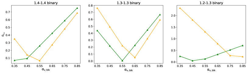
Figure 9: $\epsilon_{L_{\nu}}$ as a function of $\alpha_{\nu,\rm{blk}}\in[0.35,0.45,0.55,0.65,0.75,0.85]$, for the three binary setups and for both electron neutrinos (green curve) and anti-neutrinos (orange curve). Plots are obtained with $\tau_{\rm{cut}}=10$ for all binaries, and with $p=2$ and $p=4$ for equal and unequal mass binaries respectively. For each binary, the value of the blocking corresponding to the minimum $\epsilon_{L_{i}}$ is lower for $i=\nu_{e}$ than for $i=\bar{\nu}_{e}$. While for $\alpha_{\nu_{e},\rm{blk}}=0.45$ $\epsilon_{L_{\nu_{e}}}\lesssim 20\%$ in all binaries, for the anti-neutrinos the larger variability of $\epsilon_{L_{\bar{\nu}_{e}}}$ with $\alpha_{\bar{\nu}_{e},\rm{blk}}$ when exploring different cases leads to a different fiducial value for equal and unequal mass binaries. In particular, $\alpha_{\bar{\nu}_{e},\rm{blk}}=0.55$ for the former case, and $\alpha_{\bar{\nu}_{e},\rm{blk}}=0.75$ for the latter case. In this way, $\epsilon_{L_{\bar{\nu}_{e}}}\lesssim 20\%$ and $\epsilon_{L_{\bar{\nu}_{e}}}<30\%$ respectively.

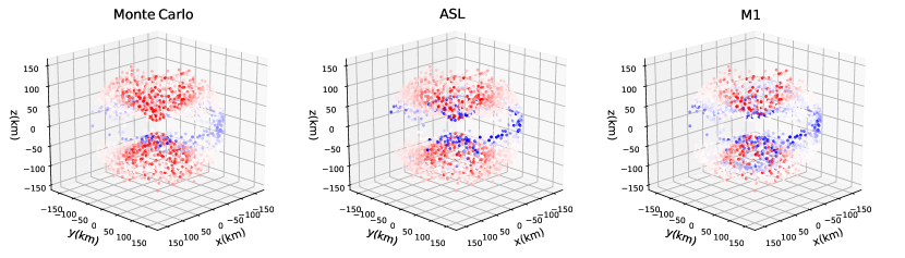
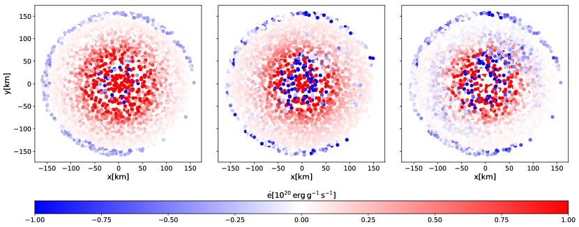
Figure 10: 3D maps (top row) and projection of the 3D maps on the x-y plane (bottom row) of the rate of change of the internal energy $\dot{e}$ in the winds (units of $10^{20}\>\rm{erg}\>\rm{g}^{-1}\>\rm{s}^{-1}$) for Sedonu (left column), the ASL (middle column) and M1 (right column), case 1). The ASL performance is similar to M1, and they both generally reproduce the distribution of $\dot{e}$ from Sedonu. The main difference with respect to Sedonu is in somewhat lower $\dot{e}>0$ and stronger $\dot{e}<0$ locally. The domain size is $x\times y\times z=150\>\rm{km}\times 150\>\rm{km}\times 150\>\rm{km}$. The map for the ASL is obtained with the parameter set $\alpha_{\nu_{e},\rm{blk}}=0.45,\alpha_{\bar{\nu}_{e},\rm{blk}}=0.55,\tau_{\rm{cut}}=10,p=2$.

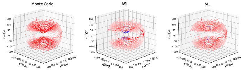
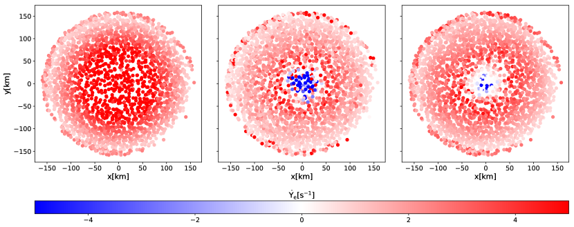
Figure 11: 3D maps (top row) and projection of the 3D maps on the x-y plane (bottom row) of the rate of change of the electron fraction $\dot{Y}_{\rm{e}}$ in the winds for Sedonu (left column), the ASL (middle column) and M1 (right column). The ASL performance is very similar to M1, and they both generally reproduce the distribution of $\dot{Y}_{\rm{e}}$ from Sedonu. The latter provides always $\dot{Y}_{\rm{e}}>0$, while both the ASL and M1 show a few particles with $\dot{Y}_{\rm{e}}<0$. Moreover, $\dot{Y}_{\rm{e}}>0$ from Sedonu appears stronger than in the ASL and M1. The domain size is $x\times y\times z=150\>\rm{km}\times 150\>\rm{km}\times 150\>\rm{km}$. The map for the ASL is obtained with the parameter set $\alpha_{\nu_{e},\rm{blk}}=0.45,\alpha_{\bar{\nu}_{e},\rm{blk}}=0.55,\tau_{\rm{cut}}=10,p=2$.

6 Conclusions

In this paper we have provided a detailed calibration analysis of the Advanced Spectral Leakage (ASL) scheme presented earlier in Gizzi et al. (2019), which is based on the original work of Perego et al. (2016). Our main motivation is the study of neutrino-driven winds emerging from neutron star mergers. The gauging process is performed by post-processing a number of snapshots of a binary neutron star merger remnant. We extract neutrino quantities directly impacted by each parameter, and we compare the ASL results for different parameter combinations with the ones obtained from the Monte Carlo neutrino transport code Sedonu (Richers et al., 2015) and from a two-moment scheme (M1) implemented in FLASH (Fryxell et al., 2000; O’Connor, 2015; O’Connor & Couch, 2018). In the calibration process we focus on electron-type neutrinos and anti-neutrinos, since they determine the properties of neutrino-driven winds. We summarise our main findings as follows:

$\bullet$ Performing neutrino transport in 2D by post-processing initial 3D post-merger configurations is of limited accuracy at early ($t\lesssim 20$ ms) times post-merger. In particular, the 2D averaging can severely impact the total luminosities by more than a factor of 2.

$\bullet$ The assumption of axially symmetric neutrino fluxes entering the heating rate in the ASL is validated by 3D neutrino transport simulations. In particular, variations of the fluxes with the azimuthal angle $\phi$ and for a given polar angle $\theta$ are limited in the bulk region of neutrino-driven winds.

$\bullet$ In agreement with Perego et al. (2016), the thermalization parameter $\tau_{\rm{cut}}$ has an impact mainly on the neutrino mean energies. However, a value of $\tau_{\rm{cut}}=10$ robustly recovers neutrino mean energies within $\lesssim 25\%$ accuracy.

$\bullet$ The heating parameter introduced in Gizzi et al. (2019) is re-calibrated to a lower value, as a result of the usage of Sedonu as reference solution. We find $p=2$ to best reproduce the distribution of the neutrino fluxes in all the cases examined. Using a M1 scheme rather than Sedonu would lead to the artifact of a larger $p$ than the ones calibrated here because of the approximations introduced by the analytical closure.

$\bullet$ The blocking parameter $\alpha_{\rm{blk}}$ mainly impacts the total neutrino luminosities, in agreement with the results of Perego et al. (2016). Moreover, unlike the other two parameters it is the most sensitive to a change of binary configuration.

$\bullet$ The assumption $\alpha_{\rm{blk}}\equiv\alpha_{\nu_{e},\rm{blk}}=\alpha_{\bar{\nu}_{e},\rm{blk}}$ adopted in Perego et al. (2016) can be rather inaccurate for recovering neutrino luminosities. In particular, electron neutrino luminosities are lower by up to a factor of 2 with respect to the reference solution, suggesting $\alpha_{\nu_{e},\rm{blk}}<\alpha_{\bar{\nu}_{e},\rm{blk}}$.

$\bullet$ Assuming $\alpha_{\nu_{e},\rm{blk}}\neq\alpha_{\bar{\nu}_{e},\rm{blk}}$, we indeed find that $\alpha_{\nu_{e},\rm{blk}}=0.45$ provides electron neutrino luminosities in agreement with the reference solution at the level of $\lesssim 20\%$ accuracy, for both equal and unequal mass binaries. Similarly, $\alpha_{\bar{\nu}_{e},\rm{blk}}=0.55$ results in electron anti-neutrino luminosities off by $\lesssim 20\%$ for equal mass binaries.

$\bullet$ We find $\alpha_{\bar{\nu}_{e},\rm{blk}}=0.75$ for unequal mass binaries, leading to a relative error in the anti-neutrino luminosity of $<30\%$. However, more test cases might be needed for a more robust evaluation and to reduce systematics.

$\bullet$ In contrast to Foucart et al. (2020), the heavy-lepton neutrino luminosity is systematically larger by a factor of a few in both the ASL and M1 with respect to an exact solution to the transport. This enhances the overall cooling of the remnant in our snapshot calculations. For the ASL, the most probable explanation is the poor treatment of the diffusion timescale, which according to Ardevol-Pulpillo et al. (2019) can boost luminosities by more than a factor of 2. We expect this treatment to affect also the electron neutrino and anti-neutrino luminosities to some extent.

$\bullet$ The properties of neutrino-driven winds are shaped by the rates of change of internal energy and electron fraction, $\dot{e}$ and $\dot{Y}_{e}$, respectively. The corresponding maps for a 1.4-1.4 $M_{\odot}$ binary demonstrate that for our suggested parameter choice the ASL scheme performs similar to the M1 approach. From the perspective of dynamical simulations, our SPH-ASL comes with the advantage of a better efficiency. In particular, by taking the Lagrangian hydrodynamics code MAGMA2 (Rosswog, 2020), we estimate that the ratio between the CPU hours spent for the transport and those spent for the hydrodynamics would be $\lesssim 0.8$ per timestep, while for the M1 in FLASH is about 10. In other words, the ASL scheme could be applied in SPH simulations with only a moderate additional computational effort.

Although the geometry of a binary neutron star merger allows neutrinos to escape with more directional freedom than in a spherically symmetric core-collapse supernova, the results we find here show that the blocking parameter can still be quite high in merger remnants. Apart from the different thermodynamics and composition of the matter, the major reason is the disk geometry that increases the effect of inward neutrino fluxes at the neutrino surfaces with respect to a spherically symmetric geometry. In this paper we have also presented a completely mesh-free, particle-based algorithm to compute spectral, species-dependent optical depths, based on the Smoothed-Particle Hydrodynamics (SPH) (Monaghan, 1992, 2005; Rosswog, 2009, 2015a, 2015b, 2020). This algorithm makes our ASL fully grid-independent, and therefore suitable for future SPH dynamical simulations of binary neutron star mergers with neutrino transport.

Data Availability

The data concerning the initial conditions needed to run the simulations, as well as the extracted neutrino quantities from all neutrino transport codes and neutrino-driven wind maps are available from the authors of this manuscript upon request.

References

- Abbott et al. (2017a) Abbott B. P., et al., 2017a, Physical Review Letters, 119, 161101
- Abbott et al. (2017b) Abbott B. P., et al., 2017b, Nature, 551, 85
- Abbott et al. (2017c) Abbott B. P., et al., 2017c, ApJ, 848, L12
- Abbott et al. (2018) Abbott B. P., et al., 2018, Physical Review Letters, 121, 161101
- Abdikamalov et al. (2012) Abdikamalov E., et al., 2012, The Astrophysical Journal, 755, 111
- Arcavi et al. (2017) Arcavi I., et al., 2017, Nature, 551, 64
- Ardevol-Pulpillo et al. (2019) Ardevol-Pulpillo R., Janka H. T., Just O., Bauswein A., 2019, MNRAS, 485, 4754
- Audit et al. (2002) Audit E., et al., 2002, arXiv e-prints, pp astro–ph/0206281
- Bauswein et al. (2017) Bauswein A., Just O., Janka H.-T., Stergioulas N., 2017, The Astrophysical Journal, 850, L34
- Bernuzzi et al. (2020) Bernuzzi S., et al., 2020, MNRAS, 497, 1488
- Bruenn (1985) Bruenn S. W., 1985, ApJS, 58, 771
- Bruenn et al. (1978) Bruenn S. W., Buchler J. R., Yueh W. R., 1978, Ap&SS, 59, 261
- Burrows & Thompson (2004) Burrows A., Thompson T. A., 2004, in Fryer C. L., ed., Astrophysics and Space Science Library Vol. 302, Astrophysics and Space Science Library. pp 133–174, doi:10.1007/978-0-306-48599-2_5
- Cabezón et al. (2018) Cabezón R. M., Pan K.-C., Liebendörfer M., Kuroda T., Ebinger K., Heinimann O., Perego A., Thielemann F.-K., 2018, A&A, 619, A118
- Castor (2004) Castor J. I., 2004, Radiation Hydrodynamics. Cambridge University Press, doi:10.1017/CBO9780511536182
- Chornock et al. (2017) Chornock R., et al., 2017, ApJL, 848, L19
- Ciolfi & Kalinani (2020) Ciolfi R., Kalinani J. V., 2020, ApJ, 900, L35
- Ciolfi et al. (2017) Ciolfi R., Kastaun W., Giacomazzo B., Endrizzi A., Siegel D. M., Perna R., 2017, Phys. Rev. D, 95, 063016
- Coughlin et al. (2019) Coughlin M. W., Dietrich T., Margalit B., Metzger B. D., 2019, MNRAS, 489, L91
- Coulter et al. (2017) Coulter D. A., et al., 2017, Science, 358, 1556
- Curtis et al. (2019) Curtis S., et al., 2019, ApJ, 870, 2
- De et al. (2018) De S., Finstad D., Lattimer J., et al., 2018, Phys. Rev. Lett., 121, 091102
- Dessart et al. (2009) Dessart L., Ott C. D., Burrows A., Rosswog S., Livne E., 2009, ApJ, 690, 1681
- Dhawan et al. (2020) Dhawan S., Bulla M., Goobar A., et al., 2020, The Astrophysical Journal, 888, 67
- Drout et al. (2017) Drout M. R., et al., 2017, Science, 358, 1570
- Ebinger et al. (2020a) Ebinger K., et al., 2020a, ApJ, 888, 91
- Ebinger et al. (2020b) Ebinger K., et al., 2020b, ApJ, 888, 91
- Eichler et al. (1989) Eichler D., Livio M., Piran T., Schramm D. N., 1989, Nature, 340, 126
- Endrizzi et al. (2020) Endrizzi A., et al., 2020, European Physical Journal A, 56, 15
- Evans et al. (2017) Evans P. A., et al., 2017, Science, 358, 1565
- Fernández & Metzger (2013) Fernández R., Metzger B. D., 2013, MNRAS, 435, 502
- Fernández et al. (2019) Fernández R., Tchekhovskoy A., Quataert E., Foucart F., Kasen D., 2019, MNRAS, 482, 3373
- Foucart et al. (2016) Foucart F., O’Connor E., Roberts L., Kidder L. E., Pfeiffer H. P., Scheel M. A., 2016, Phys. Rev. D, 94, 123016
- Foucart et al. (2018) Foucart F., Duez M. D., Kidder L. E., Nguyen R., Pfeiffer H. P., Scheel M. A., 2018, Phys. Rev. D, 98, 063007
- Foucart et al. (2020) Foucart F., Duez M. D., Hebert F., Kidder L. E., Pfeiffer H. P., Scheel M. A., 2020, ApJ, 902, L27
- Freiburghaus et al. (1999) Freiburghaus C., Rosswog S., Thielemann F.-K., 1999, ApJ, 525, L121
- Fryxell et al. (2000) Fryxell B., et al., 2000, ApJS, 131, 273
- Fujibayashi et al. (2018) Fujibayashi S., et al., 2018, The Astrophysical Journal, 860, 64
- Fujibayashi et al. (2020) Fujibayashi S., et al., 2020, Phys. Rev. D, 101, 083029
- Gafton & Rosswog (2011) Gafton E., Rosswog S., 2011, MNRAS, 418, 770
- George et al. (2020) George M., et al., 2020, arXiv e-prints, p. arXiv:2009.04046
- Gizzi et al. (2019) Gizzi D., O’Connor E., Rosswog S., Perego A., Cabezón R. M., Nativi L., 2019, MNRAS, 490, 4211
- Goldstein et al. (2017) Goldstein A., et al., 2017, ApJ, 848, L14
- Hannestad & Raffelt (1998) Hannestad S., Raffelt G., 1998, The Astrophysical Journal, 507, 339
- Janka (1992) Janka H. T., 1992, A&A, 256, 452
- Janka & Hillebrandt (1989a) Janka H. T., Hillebrandt W., 1989a, A&AS, 78, 375
- Janka & Hillebrandt (1989b) Janka H. T., Hillebrandt W., 1989b, A&A, 224, 49
- Jiang et al. (2019) Jiang J.-L., et al., 2019, The Astrophysical Journal, 885, 39
- Jiang et al. (2020) Jiang J.-L., et al., 2020, The Astrophysical Journal, 892, 55
- Kasen et al. (2013) Kasen D., Badnell N. R., Barnes J., 2013, ApJ, 774, 25
- Kasen et al. (2017) Kasen D., Metzger B., Barnes J., Quataert E., Ramirez-Ruiz E., 2017, Nature, 551, 80
- Kasliwal et al. (2017) Kasliwal M. M., Nakar E., Singer L. P., Kaplan D. L., et al. 2017, Science, 358, 1559
- Keil et al. (2003) Keil M. T., Raffelt G. G., Janka H.-T., 2003, ApJ, 590, 971
- Kilpatrick et al. (2017) Kilpatrick C. D., et al., 2017, Science, 358, 1583
- Kiuchi et al. (2019) Kiuchi K., Kyutoku K., Shibata M., Taniguchi K., 2019, The Astrophysical Journal, 876, L31
- Korobkin et al. (2012) Korobkin O., Rosswog S., Arcones A., Winteler C., 2012, MNRAS, 426, 1940
- Lattimer & Schramm (1974) Lattimer J. M., Schramm D. N., 1974, ApJ, (Letters), 192, L145
- Levermore & Pomraning (1981) Levermore C. D., Pomraning G. C., 1981, ApJ, 248, 321
- Liebendörfer et al. (2009) Liebendörfer M., Whitehouse S. C., Fischer T., 2009, The Astrophysical Journal, 698, 1174
- Lindquist (1966) Lindquist R. W., 1966, Annals of Physics, 37, 487
- Lippuner & Roberts (2015) Lippuner J., Roberts L. F., 2015, ApJ, 815, 82
- Lipunov et al. (2017) Lipunov V. M., et al., 2017, ApJ, 850, L1
- Martin et al. (2015) Martin D., et al., 2015, The Astrophysical Journal, 813, 2
- Mezzacappa & Messer (1999) Mezzacappa A., Messer O. E. B., 1999, Journal of Computational and Applied Mathematics, 109, 281
- Minerbo (1978) Minerbo G. N., 1978, J. Quant. Spectrosc. Radiative Transfer, 20, 541
- Monaghan (1992) Monaghan J. J., 1992, Ann. Rev. Astron. Astrophys., 30, 543
- Monaghan (2005) Monaghan J. J., 2005, Reports on Progress in Physics, 68, 1703
- Most et al. (2018) Most E. R., Weih L. R., Rezzolla L., Schaffner-Bielich J., 2018, Physical Review Letters, 120, 261103
- Narayan et al. (1992) Narayan R., Paczynski B., Piran T., 1992, The Astrophysical Journal, 395, L83
- Nedora et al. (2019) Nedora V., Bernuzzi S., Radice D., Perego A., Endrizzi A., Ortiz N., 2019, ApJ, 886, L30
- Nedora et al. (2020) Nedora V., et al., 2020, arXiv e-prints, p. arXiv:2008.04333
- O’Connor (2015) O’Connor E., 2015, ApJS, 219, 24
- O’Connor & Couch (2018) O’Connor E. P., Couch S. M., 2018, The Astrophysical Journal, 854, 63
- O’Connor & Ott (2010) O’Connor E., Ott C. D., 2010, Classical and Quantum Gravity, 27, 114103
- O’Connor & Ott (2013) O’Connor E., Ott C. D., 2013, ApJ, 762, 126
- O’Connor et al. (2018) O’Connor E., et al., 2018, Journal of Physics G Nuclear Physics, 45, 104001
- Obergaulinger et al. (2014) Obergaulinger M., Janka H. T., Aloy M. A., 2014, MNRAS, 445, 3169
- Paczynski (1986) Paczynski B., 1986, The Astrophysical Journal, 308, L43
- Pan et al. (2018) Pan K.-C., Mattes C., O’Connor E. P., Couch S. M., Perego A., Arcones A., 2018, Journal of Physics G: Nuclear and Particle Physics, 46, 014001
- Perego et al. (2014a) Perego A., Rosswog S., Cabezón R. M., Korobkin O., Käppeli R., Arcones A., Liebendörfer M., 2014a, MNRAS, 443, 3134
- Perego et al. (2014b) Perego A., Gafton E., Cabezón R., Rosswog S., Liebendörfer M., 2014b, A&A, 568, A11
- Perego et al. (2016) Perego A., Cabezón R. M., Käppeli R., 2016, ApJS, 223, 22
- Perego et al. (2019) Perego A., Bernuzzi S., Radice D., 2019, European Physical Journal A, 55, 124
- Pian et al. (2017) Pian E., et al., 2017, Nature, 551, 67
- Pons et al. (2000) Pons J. A., Ibáñez J. M., Miralles J. A., 2000, MNRAS, 317, 550
- Radice & Dai (2019) Radice D., Dai L., 2019, European Physical Journal A, 55, 50
- Radice et al. (2018a) Radice D., Perego A., Zappa F., Bernuzzi S., 2018a, ApJ, 852, L29
- Radice et al. (2018b) Radice D., Perego A., Hotokezaka K., Fromm S. A., Bernuzzi S., Roberts L. F., 2018b, The Astrophysical Journal, 869, 130
- Richers (2020) Richers S., 2020, Phys. Rev. D, 102, 083017
- Richers et al. (2015) Richers S., Kasen D., O’Connor E., Fernández R., Ott C. D., 2015, ApJ, 813, 38
- Rosswog (2009) Rosswog S., 2009, New Astron. Rev., 53, 78
- Rosswog (2015a) Rosswog S., 2015a, Living Reviews of Computational Astrophysics (2015), 1
- Rosswog (2015b) Rosswog S., 2015b, MNRAS, 448, 3628
- Rosswog (2020) Rosswog S., 2020, MNRAS, 498, 4230
- Rosswog & Liebendörfer (2003) Rosswog S., Liebendörfer M., 2003, MNRAS, 342, 673
- Rosswog et al. (1999) Rosswog S., Liebendörfer M., Thielemann F.-K., Davies M., Benz W., Piran T., 1999, A & A, 341, 499
- Rosswog et al. (2000) Rosswog S., et al., 2000, A&A, 360, 171
- Rosswog et al. (2017) Rosswog S., Feindt U., Korobkin O., Wu M. R., Sollerman J., Goobar A., Martinez-Pinedo G., 2017, Classical and Quantum Gravity, 34, 104001
- Rosswog et al. (2018) Rosswog S., Sollerman J., Feindt U., Goobar A., Korobkin O., Wollaeger R., Fremling C., Kasliwal M. M., 2018, A&A, 615, A132
- Savchenko et al. (2017) Savchenko V., et al., 2017, ApJ, 848, L15
- Siegel & Metzger (2017) Siegel D. M., Metzger B. D., 2017, Phys. Rev. Lett., 119, 231102
- Skinner et al. (2019) Skinner M. A., Dolence J. C., Burrows A., Radice D., Vartanyan D., 2019, ApJS, 241, 7
- Smartt et al. (2017) Smartt S. J., et al., 2017, Nature, 551, 75
- Smit et al. (1997) Smit J. M., Cernohorsky J., Dullemond C. P., 1997, A&A, 325, 203
- Soares-Santos et al. (2017) Soares-Santos M., et al., 2017, The Astrophysical Journal, 848, L16
- Steiner et al. (2013) Steiner A. W., Hempel M., Fischer T., 2013, ApJ, 774, 17
- Tanaka & Hotokezaka (2013) Tanaka M., Hotokezaka K., 2013, ApJ, 775, 113
- Vincent et al. (2020) Vincent T., et al., 2020, Phys. Rev. D, 101, 044053