Variational Inference for Shrinkage Priors: The R package vir

Abstract

We present vir, an R package for variational inference with shrinkage priors. Our package implements variational and stochastic variational algorithms for linear and probit regression models, the use of which is a common first step in many applied analyses. We review variational inference and show how the derivation for a Gibbs sampler can be easily modified to derive a corresponding variational or stochastic variational algorithm. We provide simulations showing that, at least for a normal linear model, variational inference can lead to similar uncertainty quantification as the corresponding Gibbs samplers, while estimating the model parameters at a fraction of the computational cost. Our timing experiments show situations in which our algorithms converge faster than the frequentist LASSO implementations in glmnet while simultaneously providing superior parameter estimation and variable selection. Hence, our package can be utilized to quickly explore different combinations of predictors in a linear model, while providing accurate uncertainty quantification in many applied situations. The package is implemented natively in R and RcppEigen, which has the benefit of bypassing the substantial operating system specific overhead of linking external libraries to work efficiently with R.

Keywords: Bayesian statistics, big data, Gibbs sampling, shrinkage priors, variational inference

1 Introduction

Bayesian statistics assumes that all information about a parameter of interest is contained in a probability distribution called the posterior. In most modern problems, the posterior is hard to compute due to an intractable normalizing constant, and approximations to it are necessary to conduct inference. The most popular choice for approximating the posterior distribution has been the use of Markov Chain Monte Carlo (MCMC) algorithms (Robert and Casella, 2013). MCMC algorithms work by constructing a Markov chain which has the posterior as its stationary distribution. Once the stationary distribution is reached, samples collected from chain serve as an approximation of the posterior distribution.

A variety of MCMC algorithms exist, with the two most important being the Metropolis-Hastings algorithm (Metropolis et al., 1953; Hastings, 1970) and the Gibbs sampler (Geman and Geman, 1984; Gelfand and Smith, 1990). The use of these algorithms is simplified by software which implement them in an automatic fashion by allowing the user to define a model; the R packages rjags (Plummer et al., 2019) and r2winbugs (Sturtz et al., 2005) implement Gibbs samplers, while the package rstan (Stan Development Team, 2018) uses the No-U-Turn sampler (Hoffman and Gelman, 2014) for Hamiltonian Monte Carlo (Betancourt, 2017).

Unfortunately, an issue with MCMC based approaches is that they scale poorly with dataset size or when the number of parameters is large. Consequently, modern work in MCMC has focused on dealing with these limitations. To name a few, these methods work by exploiting modern computing architecture such as GPUs (Terenin et al., 2019), splitting the dataset into smaller chunks (data sharding) and running independent chains asynchronously (Terenin et al., 2020) or combining the results after convergence (Scott et al., 2016; Srivastava et al., 2015), compressing the data before analysis (Guhaniyogi and Dunson, 2015), sub-sampling data to approximate expensive likelihoods (Quiroz et al., 2018; Ma et al., 2015), or using low-rank proposals for high dimensional parameter spaces (Saibaba et al., 2019). Most of these approaches are not readily available for use in statistical software, something which inhibits the use of the Bayesian paradigm in many applied problems of interest.

An alternative to sampling based approaches for posterior approximation is to use variational inference (VI) (Blei et al., 2017a), which casts the problem into an optimization framework. The main idea is to find an optimal distribution from a family of densities which is closest to the posterior based on some distance measure, where the family is chosen to balance computational tractability and the quality of the posterior approximation. Since variational inference is an optimization based approach, it has the advantage that it can be easily scaled to large data sets using stochastic optimization (Hoffman et al., 2013). At present, only a few R packages exist which implement variational methods: rstan, which utilizes the STAN framework to implement automatic differentiation variational inference (ADVI), but includes a warning that their implementation is unstable and subject to change (Stan Development Team, 2018; Kucukelbir et al., 2017), and the package varbvs (Carbonetto et al., 2012), which incorporates methods for variable selection using spike-and-slab priors for normal and logistic linear models.

In this chapter we present a new R package vir, which includes a set of variational and stochastic variational algorithms to estimate parameters in linear and probit regression with shrinkage priors. We incorporate the normal (ridge), double-exponential (LASSO) (Park and Casella, 2008), and horseshoe (Carvalho et al., 2010) priors to conduct variable selection and inference, a problem which arises as a first step in almost all applied analyses. Our package adds to the R ecosystem by providing a suite of computationally efficient variational algorithms, which scale with both the number of parameters, by allowing independence assumptions between regression coefficients, and the number of data points, by utilizing stochastic optimization methods. We implement the algorithms natively in R and RcppEigen, which has the benefit of bypassing the substantial operating system specific overhead of linking external libraries to work efficiently with R. Through our simulation studies, we show that the variational algorithms presented in this chapter are competitive with the popular glmnet package (Simon et al., 2011), which is widely used for variable selection, in both computation time and variable selection accuracy. Additionally, our simulation studies calculate empirical coverage probabilities for the regression coefficients, showing that the variational algorithms have the potential to recover the correct coverage in many applied scenarios.

The rest of this chapter proceeds as follows: Section 2 provides a short review of Gibbs sampling, Section 3 reviews relevant details for variational and stochastic variational inference, Section 4 reviews the use and implementation of our package, Sections 5 and 6 contain numerical studies comparing vir with glmnet, and Section 7 provides a short discussion of our results.

2 Markov Chain Monte Carlo Methods

As discussed in Section 1, the core problem in conducting Bayesian inference for a parameter, ${{\bm{\mathbf{{\theta}}}}}$, is the calculation of its posterior distribution conditioned on the data, ${\bf y}$: $p({{\bm{\mathbf{{\theta}}}}}|{\bf y})$. This quantity is rarely available in closed form, and approximations to it are necessary to estimate functions of ${{\bm{\mathbf{{\theta}}}}}$ that may be of interest. The variational algorithms implemented in this package are an example of such approximation algorithms, but their use in the Bayesian literature pales in comparison to the use of Markov Chain Monte Carlo (MCMC) methods. In this section, we focus our discussion of MCMC on Gibbs sampling because of its close relationship with variational inference: the derivations necessary to derive and implement a Gibbs sampler can be extended to derive the corresponding variational algorithms. For a comprehensive treatment of MCMC algorithms, we refer the reader to Robert and Casella (2013) and Brooks et al. (2011).

2.1 Gibbs Sampling

Gibbs sampling is one of the most popular MCMC algorithms in use today. It is a widely applicable special case of the Metropolis-Hastings algorithm and is straightforward to use when the full conditional distributions of each parameter are easy to sample from.

To understand how these algorithms are implemented, first note that the posterior distribution, $p({{\bm{\mathbf{{\theta}}}}}|{\bf y})$ can also be written as $p(\theta_{1},\dots,\theta_{P}|{\bf y})$. We then choose an initial state of the Markov chain for ${{\bm{\mathbf{{\theta}}}}}$, $(\theta_{1}^{(0)},\dots,\theta_{P}^{(0)})$ and update this state one element at a time by sampling from its full conditional, the distribution of that parameter conditioned on all others. If we continue this procedure for many iterations, updating each element one at a time in no particular order, the Markov chain will converge to the posterior distribution of interest, and storing the state at the end of each iteration after a ‘burn-in’ period will give us approximate draws from $p({{\bm{\mathbf{{\theta}}}}}|{\bf y})$; the full description of the algorithm is given in Algorithm 1. An important technique to allow the use of a Gibbs sampler in a model is to use conjugate priors for the parameters, which lead to each full conditional being of the same form as the prior distribution. All the models we consider in this chapter have priors with this conjugate relationship.

Result: Samples from a posterior approximation

Input: Integers: burn_in and n_iter, with $\texttt{burn\_in}<\texttt{n\_iter}$

Set ${{\bm{\mathbf{{\theta}}}}}^{(0)}=(\theta_{1}^{(0)},\dots,\theta_{P}^{(0)})$ ;

for $i\leftarrow 0$ to n_iter do

       $\theta_{1}^{(i+1)}\sim p(\theta_{1}|\theta_{2}^{(i)},\theta_{3}^{(i)},\dots,\theta_{P}^{(i)})$;

       $\theta_{2}^{(i+1)}\sim p(\theta_{2}|\theta_{1}^{(i+1)},\theta_{3}^{(i)},\dots,\theta_{P}^{(i)})$;

       ⋮$\theta_{p}^{(i+1)}\sim p(\theta_{p}|\theta_{1}^{(i+1)},\theta_{2}^{(i+1)},\dots,\theta_{p-1}^{(i+1)},\theta_{p+1}^{(i)},\dots,\theta_{P}^{(i)})$;

       ⋮$\theta_{P}^{(i+1)}\sim p(\theta_{p}|\theta_{1}^{(i+1)},\dots\theta_{P-1}^{(i+1)})$;

      

end for

Output: $\left\{{{\bm{\mathbf{{\theta}}}}}^{(\texttt{burn\_in}+1)},\dots,{{\bm{\mathbf{{\theta}}}}}^{(\texttt{n\_iter})}\right\}$

Algorithm 1 Gibbs Sampler

2.1.1 Exponential Families

Finding a conjugate prior for a distribution is always possible for regular exponential families (Bernardo and Smith (2000), Proposition 5.4), where the probability density (mass) function for a random variable, ${\bf y}$, can be written in the form:

$$f({\bf y}|{{\bm{\mathbf{{\theta}}}}})=h({\bf y})\exp\left\{\langle{{\bm{\mathbf{{\delta}}}}}_{y}({{\bm{\mathbf{{\theta}}}}})|{\bf t}({\bf y})\rangle-A[{{\bm{\mathbf{{\delta}}}}}_{y}({{\bm{\mathbf{{\theta}}}}})]\right\},$$ (1)

where ${{\bm{\mathbf{{\delta}}}}}_{y}({{\bm{\mathbf{{\theta}}}}})$ is called the natural parameter of the distribution, ${\bf t}({\bf y})$ is a vector of sufficient statistics, and $\langle\cdot|\cdot\rangle$ is an inner product. It should be noted that ${\bf t}({\bf y})$ lies in a general vector space and its elements can be scalars, vectors, or matrices, with the inner product $\langle\cdot|\cdot\rangle$ defined to be the sum of the inner products of the respective spaces. For example, a $p$ dimensional multivariate normal distribution for a random variable ${\bf y}$, has sufficient statistics ${\bf y}\in\mathbb{R}^{p}$ and ${\bf y}{\bf y}^{\sf T}\in\mathbb{R}^{p\times p}$. Hence, ${\bf t}({\bf y})\in\mathbb{R}^{p}\times\mathbb{R}^{p\times p}$ with $\langle\cdot|\cdot\rangle=\langle\cdot|\cdot\rangle_{\mathbb{R}^{p}}+\langle\cdot|\cdot\rangle_{\mathbb{R}^{p\times p}}$.

For any distribution that can be written in the form of (1), there exists a conjugate prior for the parameter ${{\bm{\mathbf{{\theta}}}}}$ that can be written in the same form:

$$p({{\bm{\mathbf{{\theta}}}}}|{{\bm{\mathbf{{\alpha}}}}})=h({{\bm{\mathbf{{\theta}}}}})\exp\left\{\langle{{\bm{\mathbf{{\alpha}}}}}|{\bf t}({{\bm{\mathbf{{\theta}}}}})\rangle-A({{\bm{\mathbf{{\alpha}}}}})\right\},$$

where the sufficient statistic ${\bf t}({{\bm{\mathbf{{\theta}}}}})$ is,

$${\bf t}({{\bm{\mathbf{{\theta}}}}})=\begin{pmatrix}{{\bm{\mathbf{{\delta}}}}}_{y}({{\bm{\mathbf{{\theta}}}}})\\ -A[{{\bm{\mathbf{{\delta}}}}}_{y}({{\bm{\mathbf{{\theta}}}}})]\end{pmatrix},$$

and ${{\bm{\mathbf{{\alpha}}}}}$, the natural parameter of the prior distribution, can be partitioned into ${{\bm{\mathbf{{\alpha}}}}}=({{\bm{\mathbf{{\alpha}}}}}_{1},\alpha_{2})^{T}$, with ${{\bm{\mathbf{{\alpha}}}}}_{1}$ being of the same dimension as ${{\bm{\mathbf{{\delta}}}}}_{y}({{\bm{\mathbf{{\theta}}}}})$ and $\alpha_{2}$ being a scalar. Assuming we have $N$ independent and identically distributed samples from $f({\bf y}|{{\bm{\mathbf{{\theta}}}}})$, multiplying the likelihood with the prior we see that:

$$p({{\bm{\mathbf{{\theta}}}}}|{\bf y}_{1},\dots,{\bf y}_{N},{{\bm{\mathbf{{\alpha}}}}}) \propto\prod_{n=1}^{N}p({\bf y}_{n}|{{\bm{\mathbf{{\theta}}}}})p({{\bm{\mathbf{{\theta}}}}}|{{\bm{\mathbf{{\alpha}}}}}),$$

$$\propto\prod_{n=1}^{N}\exp\left\{\langle{{\bm{\mathbf{{\delta}}}}}_{y}({{\bm{\mathbf{{\theta}}}}})|{\bf t}({\bf y}_{n})\rangle-A[{{\bm{\mathbf{{\delta}}}}}_{y}({{\bm{\mathbf{{\theta}}}}})]\right\}h({{\bm{\mathbf{{\theta}}}}})\exp\left\{\langle{{\bm{\mathbf{{\alpha}}}}}|{\bf t}({{\bm{\mathbf{{\theta}}}}})\rangle-A({{\bm{\mathbf{{\alpha}}}}})\right\},$$

$$\propto h({{\bm{\mathbf{{\theta}}}}})\exp\left\{\langle{{\bm{\mathbf{{\delta}}}}}_{{{\bm{\mathbf{{\theta}}}}}}^{*}|{\bf t}({{\bm{\mathbf{{\theta}}}}})\rangle-A({{\bm{\mathbf{{\alpha}}}}})\right\},$$

where,

$${{\bm{\mathbf{{\delta}}}}}^{*}_{{{\bm{\mathbf{{\theta}}}}}}=\begin{pmatrix}\sum_{n=1}^{N}{\bf t}({\bf y}_{n})+{{\bm{\mathbf{{\alpha}}}}}_{1}\\ N+\alpha_{2}\end{pmatrix},$$ (2)

and we use the fact that $-A[{{\bm{\mathbf{{\delta}}}}}_{y}({{\bm{\mathbf{{\theta}}}}})]=\langle-A[{{\bm{\mathbf{{\delta}}}}}_{y}({{\bm{\mathbf{{\theta}}}}})]|1\rangle_{\mathbb{R}}$.

Such manipulations with exponential families are of critical importance when deriving variational algorithms. We will see that writing the full conditionals of a Gibbs sampler in a natural parameter exponential family form simplifies the derivation of the stochastic gradient descent algorithms implemented in the package.

3 Variational Inference

MCMC methods are known to scale poorly to large datasets, both in the number of observations ($N$) and the number of parameters ($P$). Variational Inference (Blei et al., 2017b; Bishop, 2006; Murphy, 2012) aims to alleviate these issues by approximating the probability distribution of interest by utilizing optimization instead of sampling. As will be seen in our numerical experiments in Section 5, when compared with Gibbs sampling, these methods yield similar results for many quantities of interest while approximating the posterior at a fraction of the computational cost. In the following sections we will review some of the salient details of variational inference while referring the reader to Blei et al. (2017b); Hoffman et al. (2013); Bishop (2006); Murphy (2012) for a thorough review.

3.1 General Setup

For the rest of this section, let $p({{\bm{\mathbf{{\theta}}}}}|{\bf Y})$, be the posterior distribution of interest, with ${{\bm{\mathbf{{\theta}}}}}$ being the parameter and ${\bf Y}$ being the observed data, ${\bf Y}=({\bf y}_{1},\dots,{\bf y}_{n})$. While MCMC aims to sample from this distribution, VI aims to approximate it minimizing the Kullbak-Leibler (KL) divergence using a family of candidate densities, $\mathcal{D}$. The optimization problem is:

$$\begin{split}q^{*}({{\bm{\mathbf{{\theta}}}}})&=\operatorname*{arg\,min}_{q({{\bm{\mathbf{{\theta}}}}})\in\mathcal{D}}KL\left\{q({{\bm{\mathbf{{\theta}}}}}),\ p({{\bm{\mathbf{{\theta}}}}}|{\bf Y})\right\},\\ &=\operatorname*{arg\,min}_{q({{\bm{\mathbf{{\theta}}}}})\in\mathcal{D}}\int q({{\bm{\mathbf{{\theta}}}}})\log\left\{\frac{q({{\bm{\mathbf{{\theta}}}}})}{p({{\bm{\mathbf{{\theta}}}}}|{\bf Y})}\right\}d{{\bm{\mathbf{{\theta}}}}}.\end{split}$$ (3)

By utlizing Bayes’ rule, we can write (3) as a maximization problem:

$$\begin{split}\operatorname*{arg\,min}_{q({{\bm{\mathbf{{\theta}}}}})\in\mathcal{D}}KL\left\{q({{\bm{\mathbf{{\theta}}}}}),\ p({{\bm{\mathbf{{\theta}}}}}|{\bf Y})\right\}&=\operatorname*{arg\,min}_{q({{\bm{\mathbf{{\theta}}}}})\in\mathcal{D}}\left\{\mathbb{E}_{q}[\log q({{\bm{\mathbf{{\theta}}}}})]-\mathbb{E}_{q}[\log p({{\bm{\mathbf{{\theta}}}}}|{\bf Y})]\right\},\\ &=\operatorname*{arg\,min}_{q({{\bm{\mathbf{{\theta}}}}})\in\mathcal{D}}\left\{\mathbb{E}_{q}[\log q({{\bm{\mathbf{{\theta}}}}})]-\mathbb{E}_{q}[\log p({{\bm{\mathbf{{\theta}}}}},{\bf Y})]+\log p({\bf Y})\right\},\\ &=\operatorname*{arg\,min}_{q({{\bm{\mathbf{{\theta}}}}})\in\mathcal{D}}\left\{\mathbb{E}_{q}[\log q({{\bm{\mathbf{{\theta}}}}})]-\mathbb{E}_{q}[\log p({{\bm{\mathbf{{\theta}}}}},{\bf Y})]\right\},\\ &=\operatorname*{arg\,max}_{q({{\bm{\mathbf{{\theta}}}}})\in\mathcal{D}}\left\{\mathbb{E}_{q}[\log p({{\bm{\mathbf{{\theta}}}}},{\bf Y})]-\mathbb{E}_{q}[\log q({{\bm{\mathbf{{\theta}}}}})]\right\},\end{split}$$ (4)

where the second to last line drops $\log p({\bf Y})$ because it does not depend on ${{\bm{\mathbf{{\theta}}}}}$ and the last multiplies the equation by negative one. We call the term being maximized in (4) the evidence lower bound (ELBO) because it is a lower bound for the marginal distribution of ${\bf Y}$, $p({\bf Y})$, also called the evidence in the machine learning literature (Blei et al., 2017b).

3.2 Mean-Field Approximations

The tractability of the optimization problem depends on the family of densities under consideration; the more complicated the family of densities the harder the optimization problem will become. Additionally, once we find the optimal density, we will need to calculate expectations and quantiles with respect to it, which pushes us towards simpler approximations. One of the most popular families to use in variational inference is to assume that the distribution of subsets of the parameter vector, ${{\bm{\mathbf{{\theta}}}}}=({{\bm{\mathbf{{\theta}}}}}^{T}_{1},\dots,{{\bm{\mathbf{{\theta}}}}}^{T}_{P})^{T}$, are independent, where the subsets are chosen for computational convenience. Hence,

$$\mathcal{D}=\left\{q({{\bm{\mathbf{{\theta}}}}}):q({{\bm{\mathbf{{\theta}}}}})=\prod_{p=1}^{P}q_{p}({{\bm{\mathbf{{\theta}}}}}_{p})\right\}.$$ (5)

The class of densities in (5) do not make an assumption regarding the optimal distributions for each ${{\bm{\mathbf{{\theta}}}}}_{p}$ except for the fact that they are independent. Additionally, the groups within ${{\bm{\mathbf{{\theta}}}}}$ can be selected to with a particular structure in mind, with a focus on grouping correlated parameters together.

3.2.1 Coordinate Ascent Variational Inference (CAVI)

Coordinate ascent is the most popular approach for finding the optimal distribution under the mean-field restrictions in (5). This approach iteratively optimizes the ELBO with respect to each factorized density, while holding all other constant. The resulting algorithm is dubbed coordinate ascent variational interference (CAVI). The derivations for the optimal density are given in various texts Bishop (2006); Blei et al. (2017b); Murphy (2012) and we state the result below for convenience. First, note that the ELBO with respect to the factor, $q_{p}({{\bm{\mathbf{{\theta}}}}}_{p})$, can be written as:

$$\begin{split}\text{ELBO}[q_{p}({{\bm{\mathbf{{\theta}}}}}_{p})]&={\bf E}_{q({{\bm{\mathbf{{\theta}}}}})}\left[\log p({{\bm{\mathbf{{\theta}}}}},{\bf Y})\right]-\sum_{j=1}^{P}{\bf E}_{q_{j}({{\bm{\mathbf{{\theta}}}}}_{j})}\left[\log q_{j}({{\bm{\mathbf{{\theta}}}}}_{j})\right],\\ &={\bf E}_{q_{p}({{\bm{\mathbf{{\theta}}}}}_{p})}\left[{\bf E}_{q_{r}({{\bm{\mathbf{{\theta}}}}}_{r})}\left\{\log p({{\bm{\mathbf{{\theta}}}}},{\bf Y})\right\}\right]-{\bf E}_{q_{p}({{\bm{\mathbf{{\theta}}}}}_{p})}\left[\log q_{p}({{\bm{\mathbf{{\theta}}}}}_{p})\right]+\text{const},\\ &=-KL\left[q_{p}({{\bm{\mathbf{{\theta}}}}}_{p}),\ \exp\left\{{\bf E}_{q_{r}({{\bm{\mathbf{{\theta}}}}}_{r})}\left[\log p({{\bm{\mathbf{{\theta}}}}},{\bf Y})\right]\right\}\right]+\text{const},\end{split}$$

where we define $q_{r}({{\bm{\mathbf{{\theta}}}}}_{r})$ as the variational distribution for the rest of the parameters: $q_{r}({{\bm{\mathbf{{\theta}}}}}_{r})=\prod_{j\neq p}^{P}q_{j}({{\bm{\mathbf{{\theta}}}}}_{j})$. Since the $KL$ divergence between two probability distributions is always positive, the negative KL divergence is maximized when the divergence between two probability densities is equal to zero. Hence the optimal variational density for the $p^{th}$ factor is:

$$q^{*}_{p}({{\bm{\mathbf{{\theta}}}}}_{p}) \propto\exp\left\{{\bf E}_{q_{r}({{\bm{\mathbf{{\theta}}}}}_{r})}\left[\log p({{\bm{\mathbf{{\theta}}}}},{\bf Y})\right]\right\},$$ (6)

$$\propto\exp\left\{{\bf E}_{q_{r}({{\bm{\mathbf{{\theta}}}}}_{r})}\left[\log p({{\bm{\mathbf{{\theta}}}}}_{p}|{{\bm{\mathbf{{\theta}}}}}_{r},{\bf Y})\right]\right\}.$$ (7)

Consequently, the optimal variational density for the $p^{th}$ coordinate is a function of the full conditional distribution the parameter, a density that is required calculation for a Gibbs sampler.

It should be noted that, in most situations, the difficulty of calculating the expectations in (6) is a direct function of the simplicity of the variational family in (5). Assuming that a larger number of parameters independently factor in the posterior simplifies the calculations of the expectations of, for example, the inner product of two vector parameters.

3.3 Stochastic Variational Inference (SVI)

If we further assume that the complete conditionals of the parameter given all others are in the exponential family (1), and require the individual factors in the mean-field family (5) to be in the same exponential family, we can scale variational inference to large datasets that do not fit in memory. This approach, termed Stochastic Variational Inference (SVI) (Hoffman et al., 2013), utilizes gradient based optimization to maximize the ELBO instead of using the coordinate ascent algorithm presented in Section 3.2. SVI compares favorable to CAVI in models that have local variables; this means that for each data point $y_{n}$ there exists a latent parameter $z_{n}$ that needs to be estimated. In such cases, both Gibbs sampling and the CAVI algorithm process the entire dataset every iteration.

For the rest of this section, we present SVI in the context of probit regression with a normal (ridge) prior. This model has the hierarchy:

$$\begin{split}y_{n}&=\mathbb{I}(z_{n}>0),\\ z_{n}&\sim\mathcal{N}({\bf x}_{n}^{\sf T}{\bf b},1),\\ {\bf b}&\sim\mathcal{N}(0,\lambda^{-1}{\bf I}),\\ \lambda&\sim\mathcal{G}(a_{\lambda},b_{\lambda}).\end{split}$$ (8)

In this situation, the observed data is $y_{n}$, and each $y_{n}$ has a corresponding local variable, $z_{n}$, which allows the use of the probit link in the calculation of $P(y_{n}=1)=\Phi({\bf x}_{n}^{\sf T}{\bf b})$ where $\Phi(\cdot)$ is the CDF of the standard normal distribution. In a Gibbs sampler and a CAVI algorithm, we would have to update each $z_{n}$ before we can update the parameter vector ${\bf b}$, estimation of which is of primary interest.

It is well known that the complete conditional distributions of the parameters in (8) are given by:

$$\begin{split}z_{n}|\cdot&\sim\begin{cases}\mathcal{N}_{+}\left({\bf x}_{n}^{\sf T}{\bf b},1\right)\text{if }y_{n}=1\\ \mathcal{N}_{-}\left({\bf x}_{n}^{\sf T}{\bf b},1\right)\text{if }y_{n}=0\\ \end{cases},\\ {\bf b}|\cdot&\sim\mathcal{N}\left(({{\bf X}^{\sf T}{\bf X}}+\lambda{\bf I})^{-1}{\bf X}^{\sf T}{\bf z},\ ({{\bf X}^{\sf T}{\bf X}}+\lambda{\bf I})^{-1}\right),\\ \lambda|\cdot&\sim\mathcal{G}\left(a_{\lambda}+\frac{P}{2},\frac{1}{2}||{\bf b}||^{2}_{2}+b_{\lambda}\right),\end{split}$$

where, for example, ${\bf b}|\cdot$ denotes the distribution of ${\bf b}$ conditioned on all other parameters in the model, ${\bf X}=({\bf x}_{1}^{\sf T},\dots,{\bf x}_{N}^{\sf T})^{\sf T}$, and $\mathcal{N}_{+}$ and $\mathcal{N}_{-}$ are truncated normal distributions on $(0,\infty)$ and $(-\infty,0]$, respectively. Consequently, under this setup, we would restrict the optimal variational distribution of ${\bf b}$ to be a normal distribution, i.e. $q_{b}({\bf b})=\mathcal{N}\left({{\bm{\mathbf{{\mu}}}}}_{b},{{\bm{\mathbf{{\Sigma}}}}}_{b}\right)$. Because the normal distribution is part of the exponential family, it can be written in the form of (1):

$$q({\bf b}|{{\bm{\mathbf{{\delta}}}}}_{b}({{\bm{\mathbf{{\theta}}}}})) =h({\bf b})\exp\left\{\langle{{\bm{\mathbf{{\delta}}}}}_{b}({{\bm{\mathbf{{\theta}}}}})|{\bf t}_{b}({\bf b})\rangle-A\left[{{\bm{\mathbf{{\delta}}}}}_{b}({{\bm{\mathbf{{\theta}}}}})\right]\right\},$$ (9)

where,

$${\bf t}({\bf b}) =\begin{pmatrix}{\bf b}\\ {\bf b}{\bf b}^{\sf T}\end{pmatrix}\text{ and }{{\bm{\mathbf{{\delta}}}}}_{b}({{\bm{\mathbf{{\theta}}}}})=\begin{pmatrix}-\frac{1}{2}{{\bm{\mathbf{{\Sigma}}}}}_{b}^{-1}{{\bm{\mathbf{{\mu}}}}}_{b}\\ -\frac{1}{2}{{\bm{\mathbf{{\Sigma}}}}}_{b}^{-1}\end{pmatrix}.$$ (10)

Now, looking at the full conditional for ${\bf b}$, we can also put it into exponential family form as:

$$p({\bf b}|{\bf X},{\bf z},\lambda) =h({\bf b})\exp\left\{\langle{{\bm{\mathbf{{\delta}}}}}_{b}({\bf X},{\bf z},\lambda)|{\bf t}_{b}({\bf b})\rangle-A\left[{{\bm{\mathbf{{\delta}}}}}_{b}({\bf X},{\bf z},\lambda)\right]\right\}.$$ (11)

Instead of taking the gradient of the ELBO with respect to ${{\bm{\mathbf{{\delta}}}}}_{b}({{\bm{\mathbf{{\theta}}}}})$, Hoffman et al. (2013) utilize the natural gradient (Amari, 1998), which accounts for the geometry of the parameter space. Applying their derivation for the natural gradient of the ELBO to our case (Hoffman et al. (2013) ; Equation 14), gives us the natural gradient with respect to ${{\bm{\mathbf{{\delta}}}}}_{b}({{\bm{\mathbf{{\theta}}}}})$:

$$\begin{split}\nabla_{{{\bm{\mathbf{{\delta}}}}}_{b}({{\bm{\mathbf{{\theta}}}}})}ELBO&=\mathbb{E}_{q}[{{\bm{\mathbf{{\delta}}}}}_{b}({\bf X},{\bf z},\lambda)]-{{\bm{\mathbf{{\delta}}}}}_{b}({{\bm{\mathbf{{\theta}}}}}),\\ &=\mathbb{E}_{q}\left[\begin{pmatrix}\sum_{n=1}^{N}z_{n}{\bf x}_{n}\\ \sum_{n=1}^{N}{\bf x}_{n}{\bf x}_{n}^{\sf T}+\lambda{\bf I}\end{pmatrix}\right]-{{\bm{\mathbf{{\delta}}}}}_{b}({{\bm{\mathbf{{\theta}}}}}),\\ &=\begin{pmatrix}\sum_{n=1}^{N}\mathbb{E}_{q}\left[z_{n}\right]{\bf x}_{n}\\ \sum_{n=1}^{N}{\bf x}_{n}{\bf x}_{n}^{\sf T}+\mathbb{E}_{q}\left[\lambda\right]{\bf I}\end{pmatrix}-{{\bm{\mathbf{{\delta}}}}}_{b}({{\bm{\mathbf{{\theta}}}}}).\end{split}$$ (12)

This expression can be used in a gradient descent algorithm where, at each iteration, the natural parameters of the variational distribution, ${{\bm{\mathbf{{\delta}}}}}_{b}({{\bm{\mathbf{{\theta}}}}})$, are updated using the following formula:

$$\begin{split}{{\bm{\mathbf{{\delta}}}}}_{b}({{\bm{\mathbf{{\theta}}}}})^{(t)}&={{\bm{\mathbf{{\delta}}}}}_{b}({{\bm{\mathbf{{\theta}}}}})^{(t-1)}+\rho_{t}\left[\mathbb{E}_{q}[{{\bm{\mathbf{{\delta}}}}}_{b}({\bf X},{\bf z},\lambda)]-{{\bm{\mathbf{{\delta}}}}}_{b}({{\bm{\mathbf{{\theta}}}}})^{(t-1)}\right],\\ &=(1-\rho_{t}){{\bm{\mathbf{{\delta}}}}}_{b}({{\bm{\mathbf{{\theta}}}}})^{(t-1)}+\rho_{t}\mathbb{E}_{q}[{{\bm{\mathbf{{\delta}}}}}_{b}({\bf X},{\bf z},\lambda)],\end{split}$$ (13)

where $\rho_{t}$ is a predetermined step size.

Note that the gradient in (12) requires the processing of all data points due to the summation over $N$. Instead of calculating the gradient with respect to the full data, we can calculate an approximation which is equal to full gradient in expectation, and follow the iterative procedure in (13). If the sequence of step sizes, $\rho_{t}$, meets the conditions in (14), ${{\bm{\mathbf{{\delta}}}}}_{b}({{\bm{\mathbf{{\theta}}}}})^{(t)}$ will converge to a local optimum.

$$\begin{split}\sum_{t}\rho_{t}=\infty\text{ and }\sum_{t}\rho_{t}^{2}<\infty\end{split}$$ (14)

A noisy estimate of the gradient can be calculated by using only one uniformly sampled data point replicated $N$ times. This means that the summation in (12) would change to the value for one data point multiplied by $N$; that is, the parameter update in (13) becomes:

$$\begin{split}{{\bm{\mathbf{{\delta}}}}}_{b}({{\bm{\mathbf{{\theta}}}}})^{(t)}&=(1-\rho_{t}){{\bm{\mathbf{{\delta}}}}}_{b}({{\bm{\mathbf{{\theta}}}}})^{(t-1)}+\rho_{t}\left\{N\mathbb{E}_{q}\left[{{\bm{\mathbf{{\delta}}}}}_{b}({\bf x}_{n},z_{n})\right]\right\},\end{split}$$ (15)

with

$$N\mathbb{E}_{q}\left[{{\bm{\mathbf{{\delta}}}}}_{b}({\bf x}_{n},z_{n})\right]=\begin{pmatrix}N\mathbb{E}_{q}\left[z_{n}\right]{\bf x}_{n}\\ N{\bf x}_{n}{\bf x}_{n}^{\sf T}+\mathbb{E}_{q}\left[\lambda\right]{\bf I}\end{pmatrix}.$$

Finally, while the stochastic gradient updates in (15) are only computed for one data point at a time, the methodology can be extended to process S data points simultaneously. The only difference would be to average the individual results from each data point. The update step becomes:

$$\begin{split}{{\bm{\mathbf{{\delta}}}}}_{b}({{\bm{\mathbf{{\theta}}}}})^{(t)}&=(1-\rho_{t}){{\bm{\mathbf{{\delta}}}}}_{b}({{\bm{\mathbf{{\theta}}}}})^{(t-1)}+\frac{\rho_{t}}{S}\left\{N\sum_{s\in\mathcal{S}}\mathbb{E}_{q}\left[{{\bm{\mathbf{{\delta}}}}}_{b}({\bf x}_{s},z_{s})\right]\right\},\end{split}$$

which implies that,

$$N\sum_{s\in\mathcal{S}}\mathbb{E}_{q}\left[{{\bm{\mathbf{{\delta}}}}}_{b}({\bf x}_{n},z_{n})\right]=\begin{pmatrix}N{\bf X}_{s}^{\sf T}\mathbb{E}_{q}\left[{\bf z}_{s}\right]\\ N{\bf X}_{s}^{\sf T}{\bf X}_{s}+S\mathbb{E}_{q}\left[\lambda\right]{\bf I}\\ \end{pmatrix},$$

where $\mathcal{S}$ is the set of sub-sampled data points, $S=|\mathcal{S}|$, and ${\bf X}_{s}$ and ${\bf z}_{s}$ are ${\bf X}$ and ${\bf z}$ restricted to the corresponding indices in $\mathcal{S}$.

4 Implementation and Usage

The package vir contains implementations of the CAVI and SVI algorithms for univariate and multivariate regression models with the normal and probit link. For the univariate linear models, we derive and implement a Gibbs sampler, and the CAVI and SVI algorithms for the ridge (normal), LASSO (double-exponential) (Park and Casella, 2008), and horseshoe (Carvalho et al., 2010; Makalic and Schmidt, 2015) priors, while the multivariate linear models are implemented with non-informative priors for the regression coefficients and a factor model for the covariance structure. Each function is implemented in C++ and leverages the Rcpp (Eddelbuettel and Francois, 2011) and RcppEigen (Bates et al., 2013) packages to optimize performance.

The functions in the package are named according to the link function, lm for normal linear models and probit for binary regression, followed by the shrinkage prior type: ridge, lasso, hs, uninf; and then the algorithm: gibbs, cavi, or svi. Therefore, if an analyst wishes to use the svi algorithm with a linear model and horseshoe prior, they can call the function lm_hs_svi to analyze the data. Table 1 contains a summary of the names for the functions in the package. All functions take, as arguments, a matrix of predictors, ${\bf X}$ and a vector or matrix of responses, ${\bf y}$ or ${\bf Y}$.

The variational algorithms utilize two assumptions regarding the regression coefficients. The first assumes that each regression coefficient is correlated, and sets the optimal distribution of the parameter to be a multivariate normal, that is: $q({\bf b})=\mathcal{N}\left({{\bm{\mathbf{{\mu}}}}}_{b},{{\bm{\mathbf{{\Sigma}}}}}_{b}\right)$. Alternatively, we also implement a version of the algorithm which assumes that all regression coefficients are independent, i.e., $q({\bf b})=\prod_{p=1}^{P}q(b_{p})$, where each component, $q(b_{p})$ is a univariate normal distribution. The use of these two options is problem dependent; assuming the full correlation structure may lead to superior variance estimates at the expense of slower computation time.

Table 1: List of functions implemented in the vir package. The functions have the format model_prior_algorithm. Consequently, if an analyst wishes to use a Gibbs sampler to fit a multivariate linear model with a non-informative prior then they could call the function mv_lm_uninf_gibbs(). If they wished to fit a univariate probit model with a horseshoe prior using CAVI, they would call the function probit_hs_cavi(). Each function is implemented in C++ using the RcppEigen package.

Model	Priors	Algorithms
Normal: lm Probit: probit	Ridge: ridge LASSO: lasso Horseshoe: hs	Gibbs: gibbs CAVI: cavi SVI: svi
Multivariate Normal: mv_lm Multivariate Probit: mv_probit	Non-informative: uninf

Below we provide an example use case, analyzing a simulated dataset with a univariate normal linear model (16). We first demonstrate the use of CAVI with a normal prior. As described earlier, the function to be called in this situation is lm_ridge_cavi(); the documentation for which can be seen by executing ?lm_ridge_cavi in the R console. We install the package from GitHub and start by simulating a small dataset and fitting the model.

> devtools::install_github("suchitm/vir")> library(vir)> set.seed(42)> X = matrix(nrow = 100, ncol = 5, rnorm(5 * 100))> colnames(X) = paste0("X", 1:5)> b = rnorm(5)> y = rnorm(1) + X %*% b + rnorm(100)> ridge_cavi_fit = lm_ridge_cavi(y, X, n_iter = 100, rel_tol = 0.0001) Each of the algorithms output a nested list. The first layer contains an element for each of the parameters and the ELBO, while the second lists the form of the optimal distribution (normal, gamma, etc.), and the corresponding optimal parameters. Since the normal ridge model has four parameters, the first level of the list has the names:

> names(ridge_cavi_fit)

[1] "b0"     "b"      "tau"    "lambda" "elbo" where b0 is the intercept term, b is a vector of regression coefficients, tau is the error precision, and lambda is the prior precision. The optimal distribution of the regression coefficients, ${\bf b}$, is a multivariate normal with mean, ${{\bm{\mathbf{{\mu}}}}}$, and covariance matrix, ${{\bm{\mathbf{{\Sigma}}}}}$, the names for that parameter element contain the distribution type and corresponding parameters.

> names(ridge_cavi_fit$b)

[1] "dist"      "mu"        "sigma_mat"

> ridge_cavi_fit$b$dist> ridge_cavi_fit$b$mu> round(ridge_cavi_fit$b$sigma_mat, 4)

[1] "multivariate normal"[1]  0.87668826  0.92639922  0.08866204  0.10254637 -0.75907903        [,1]    [,2]    [,3]    [,4]    [,5][1,]  0.0110 -0.0006  0.0017 -0.0006 -0.0010[2,] -0.0006  0.0144 -0.0011 -0.0005  0.0017[3,]  0.0017 -0.0011  0.0115  0.0007 -0.0010[4,] -0.0006 -0.0005  0.0007  0.0156 -0.0025[5,] -0.0010  0.0017 -0.0010 -0.0025  0.0118 These parameter estimates can be summarized via the mean and credible intervals using summary_vi().

> summary_vi(ridge_cavi_fit, level = 0.95, coef_names = colnames(X))

             Estimate      Lower       UpperIntercept -0.17491248 -0.3901667  0.04034176X1         0.87668826  0.6711879  1.08218858X2         0.92639922  0.6909048  1.16189365X3         0.08866204 -0.1218641  0.29918818X4         0.10254637 -0.1424468  0.34753954X5        -0.75907903 -0.9717937 -0.54636432 Using the model fit, one can generate estimates and corresponding credible intervals for new data by utilizing the predict_lm_vi() function.

> X_test = matrix(nrow = 5, ncol = 5, rnorm(25))> predict_lm_vi(ridge_cavi_fit, X_test)

$estimate[1] -1.0235563  2.3194540 -0.5776915 -0.6762113 -1.2336189$ci           [,1]      [,2][1,] -3.1989515 1.1518389[2,]  0.1016273 4.5372806[3,] -2.7163884 1.5610055[4,] -2.8682399 1.5158172[5,] -3.4223356 0.9550978

4.1 SVI

The are three material differences between the CAVI and SVI implementations, with the first being the stopping criteria. The CAVI algorithms use a relative tolerance criteria (rel_tol) comparing the ELBO at the current iteration with the ELBO five iterations in the past. On the other hand, the SVI algorithms do not terminate based on a stopping criteria, but will instead run until the maximum number of iterations (n_iter) is reached. For each sub-sample of the data, a noisy estimate for the ELBO is calculated and stored, which can then be used to assess convergence of the algorithms.

Second, the step sizes, $\rho_{t}$, in stochastic gradient algorithms have to follow the schedule outlined in (14). We implement two ways of meeting the necessary conditions. The default approach allows setting a constant step size via the parameter const_rhot, which keeps the step size constant for each iteration of the algorithm. Alternatively, we also allow the user to specify a schedule based on the equation $\rho_{t}=(t+\omega)^{-\kappa}$, where $\omega\geq 0$ is called a delay while $\kappa\in(0.5,1]$ is called the forgetting rate (Hoffman et al., 2013). Finally, SVI algorithms utilize sub-samples of the data, and the size of these samples has to be set via the batch_size parameter. Below we show how the corresponding SVI algorithm for normal linear regression with a normal prior can be implemented in our package; in this case we set a constant learning rate of $0.1$ and use a sub-sample of ten data points for each iteration. After fitting the model, all other operations regarding parameter summaries and predictions are identical to the CAVI exposition above.

> ridge_svi_fit = lm_ridge_svi(+   y, X, n_iter = 1000, verbose = FALSE, batch_size = 10, const_rhot = 0.1+ )

It should be noted that their exists an interaction between the batch size and the step size for any stochastic gradient descent algorithm. For our numerical experiments in Section 5, we use a constant learning rate of 0.01, which seemed to work well for our purposes. Consequently, this is the default rate for our algorithms. The choice of adaptive learning rates is an open area of research in the stochastic optimization literature (Schaul et al., 2013; Kingma and Ba, 2014) and we leave their implementation to later iterations of our package.

5 Simulations

In this section we provide a simulation study comparing the ridge and LASSO penalties implemented in glmnet, to a Gibbs sampler, and the CAVI and SVI algorithms for linear and probit regression with ridge, LASSO, and horseshoe priors. For each set of simulations we generate $D=50$ datasets for our comparisons.

5.1 Linear Regression

In this section, we simulate from the model

$${\bf y}=\bm{1}b_{0}+{\bf X}{\bf b}+{\bf e};\ {\bf e}\sim\mathcal{N}\left(\bm{0},\sigma^{2}{\bf I}\right),$$ (16)

where $b_{0}\sim\mathcal{N}(0,1)$, the $n^{th}$ row of ${\bf X}$, ${\bf x}_{n}\sim\mathcal{N}({\bm{\mathbf{{0}}}},{\bm{\mathbf{{V}}}})$, ${\bm{\mathbf{{V}}}}_{j,j^{\prime}}=cov(x_{j},x_{j^{\prime}})=0.5^{|j-j^{\prime}|}$, ${\bf b}\sim\mathcal{N}({\bm{\mathbf{{0}}}},{\bf I})$, and $\sigma^{2}$ is chosen to set the signal-to-noise ratio in the data to one. We hold the number of predictors $P$ constant at $75$, and vary the size of the dataset, $N$. We set 80% of the values in ${\bf b}$ to zero, which motivates our comparison of the shrinkage priors below.

Table 2: Simulation results for the normal linear model.

	N = 100				N = 1000				N = 5000
	MSE	Cov.	MSPE		MSE	Cov.	MSPE		MSE	Cov.	MSPE
Ridge
GLM-1SE	0.160	-	0.917		0.038	-	0.732		0.012	-	0.708
GLM-Min	0.160	-	0.913		0.039	-	0.732		0.012	-	0.707
Gibbs-Corr	0.125	0.941	0.856		0.024	0.948	0.718		0.005	0.951	0.700
CAVI-Corr	0.135	0.946	0.868		0.024	0.949	0.718		0.005	0.952	0.700
CAVI-Indep	0.122	0.913	0.853		0.024	0.871	0.718		0.005	0.871	0.700
SVI-Corr	0.135	0.946	0.866		0.026	0.943	0.721		0.008	0.893	0.703
SVI-Indep	0.122	0.913	0.854		0.025	0.868	0.720		0.006	0.819	0.704
LASSO
GLM-1SE	0.129	-	0.859		0.029	-	0.721		0.010	-	0.705
GLM-Min	0.131	-	0.864		0.029	-	0.721		0.010	-	0.705
Gibbs-Corr	0.120	0.968	0.852		0.017	0.966	0.713		0.004	0.963	0.700
CAVI-Corr	0.133	0.937	0.863		0.018	0.958	0.713		0.004	0.959	0.700
CAVI-Indep	0.106	0.901	0.833		0.017	0.911	0.712		0.004	0.897	0.700
SVI-Corr	0.129	0.938	0.859		0.019	0.952	0.714		0.006	0.908	0.701
SVI-Indep	0.091	0.917	0.814		0.014	0.930	0.709		0.005	0.877	0.701
HS
Gibbs-Corr	0.097	0.945	0.809		0.010	0.975	0.705		0.002	0.983	0.698
CAVI-Corr	0.113	0.909	0.834		0.011	0.956	0.706		0.002	0.967	0.698
CAVI-Indep	0.099	0.888	0.813		0.010	0.931	0.706		0.002	0.941	0.698
SVI-Corr	0.110	0.908	0.831		0.011	0.954	0.706		0.002	0.961	0.698
SVI-Indep	0.099	0.888	0.812		0.010	0.933	0.705		0.002	0.937	0.698

We compare the mean squared error for the coefficients (MSE), coverage for 95% credible intervals (Cov.), and the relative mean squared prediction error (MSPE) for predictions on a test set of size 500 simulated from the model in (16). The formulas to calculate our metrics are below:

$$\begin{split}\text{MSE}&=\frac{1}{DP}\sum_{d=1}^{D}\sum_{p=1}^{P}(b_{p}-\hat{b}_{p})^{2},\\ \text{MPSE}&=\sqrt{\frac{||{\bf X}{\bf b}-{\bf X}\hat{{\bf b}}||^{2}_{2}}{||{\bf X}{\bf b}||^{2}_{2}}},\\ \text{COV}&=\frac{1}{DP}\sum_{d=1}^{D}\sum_{p=1}^{P}\mathbb{I}(l_{p}\leq b_{p}\leq u_{p}),\end{split}$$

where $b_{p}$ is the true coefficient, $\hat{b}_{p}$ is the corresponding estimated value, ${\bf X}$ is the predictor matrix for the test set, and $(l_{p},u_{p})$ is the credible set for the $p^{th}$ predictor.

The results for our simulations are given in Table 2. As can be seen, all implementations of the variational algorithms are competitive with glmnet and the Gibbs sampler in regards to MSE and MSPE. The variational algorithms for linear regression with the horseshoe prior provide superior parameter estimation with respect to the LASSO or ridge priors, along with outperforming the ridge and LASSO glmnet implementations.

With regards to coverage, the variational algorithms which assume posterior independence between the regression parameters have the lowest coverage among the Bayesian approaches. However, the coverage improves as $N$ increases for the horseshoe priors, which has approximately 94% coverage for the 95% credible sets measured. On the other hand, the variational algorithms which estimate a correlated structure among the parameters seem to retain coverage similar to that of the Gibbs samplers while being estimated at a fraction of the computational cost. Therefore, while, in general variational algorithms are known to underestimate the posterior variance of the model parameters, this does not seem to be an issue in the simulation settings considered. Additionally, the SVI and CAVI algorithms perform comparably in terms of point and variance estimation, providing confidence for using SVI approaches in the context of a linear regression where the data does not fit in memory.

5.2 Probit Regression

We compare the probit regression algorithms in the package using a similar design as in Section 5.1 with the modification that $z_{n}=b_{0}+{\bf x}_{n}^{\sf T}{\bf b}$ and $P(y_{n}=1)=\Phi(z_{n})$ for the probit link or $P(y_{n}=1)=\text{expit}(z_{n})$ for the logit link. Because glmnet implements the logistic link instead of the probit, we simulate from both the logistic and probit models and compare the algorithms using only one design with $N=500$, $P=50$, and set 40 of the parameters to zero.

Table 3: Simulation results for binary regression with shrinkage priors.

	Logit				Probit
	MSE	RAND	AUC-PR		MSE	Coverage	RAND	AUC-PR
Ridge
GLM-1SE	0.079	0.673	0.881		-	-	0.673	0.924
GLM-Min	0.174	0.673	0.885		-	-	0.673	0.922
Gibbs-Corr	-	0.852	0.885		0.023	0.951	0.850	0.930
CAVI-Corr	-	0.772	0.886		0.034	0.700	0.706	0.929
CAVI-Indep	-	0.671	0.886		0.035	0.588	0.607	0.929
SVI-Corr	-	0.765	0.885		0.031	0.692	0.692	0.929
SVI-Indep	-	0.660	0.885		0.032	0.568	0.588	0.929
LASSO
GLM-1SE	0.180	0.819	0.894		-	-	0.794	0.934
GLM-Min	0.174	0.621	0.898		-	-	0.591	0.938
Gibbs-Corr	-	0.866	0.892		0.024	0.970	0.863	0.936
CAVI-Corr	-	0.811	0.895		0.016	0.782	0.790	0.939
CAVI-Indep	-	0.779	0.895		0.019	0.740	0.763	0.939
SVI-Corr	-	0.810	0.894		0.017	0.782	0.790	0.939
SVI-Indep	-	0.846	0.898		0.019	0.779	0.829	0.942
HS
Gibbs-Corr	-	0.845	0.900		0.012	0.981	0.875	0.943
CAVI-Corr	-	0.871	0.901		0.010	0.856	0.869	0.944
CAVI-Indep	-	0.869	0.901		0.010	0.845	0.873	0.944
SVI-Corr	-	0.871	0.901		0.009	0.857	0.868	0.944
SVI-Indep	-	0.868	0.901		0.009	0.845	0.870	0.944

We calculate the mean squared error for the parameter estimates for each of the algorithms when the data generating process is the same as the one assumed by the model (logistic for glmnet and probit for vir), and compare the coverage of the parameter estimates in the probit case for the Gibbs sampler and the variational algorithms. We also compare the variable selection quality of the respective algorithms by using the RAND index Rand (1971), thinking of the variable selection problem as one of calculating the dissimilarities between two cluster indicator vectors. Finally, we compare the predictive capacity of our models by using the area under the precision recall curve (AUC-PR). The results for our simulation are given in Table 3.

In both simulation settings, the Gibbs samplers remain the most consistent in terms of the RAND index. The CAVI and SVI algorithms with the horseshoe prior perform comparably to the Gibbs samplers but the variational algorithms with the ridge prior perform meaningfully worse, while the ones with the LASSO perform only slightly worse. All algorithms perform similarly in terms of AUC-PR, with the horseshoe prior being slightly better than the others.

In terms of parameter estimation in the probit simulation case, we see that the estimation quality of the variational algorithms is comparable to the Gibbs samplers for the LASSO and horseshoe priors, while being worse for the ridge prior. As with the linear regression simulations, the performance of the SVI and CAVI algorithms is similar, giving us confidence in their use for large scale regression problems.

Unfortunately, when it comes to coverage, the variational algorithms meaningfully under perform the corresponding Gibbs samplers, likely due to the mean-field assumption that the latent variables for each data point are uncorrelated with the regression coefficients. Fasano et al. (2019) show that a mean-field approach for probit regression causes the regression estimates to be shrunk towards zero, and propose a variational algorithm in the spirit of the Gibbs sampler developed by Holmes et al. (2006) to remedy the issue. However, their proposed algorithm requires the prior for the regression coefficients be fixed a-priori, and their updates for the latent variables require the whole data set. Consequently, their algorithms cannot be readily extended to the adaptive shrinkage priors considered in this article, and their CAVI algorithm cannot be easily extended to utilize stochastic optimization. Therefore, we recommend that the estimated posterior variance of the regression coefficients be viewed with skepticism for the variational algorithms and note that if one desires accurate uncertainty quantification in this situation, one may, ironically, be able to utilize the bootstrap (Chen et al., 2018).

6 Computational Performance

A motivating factor for the development of our package was the computational efficiency provided by variational methods relative to MCMC; we aimed to scale linear regression with shrinkage priors to large datasets. While it is known that variational algorithms outperform their MCMC counterparts computationally, in this section we provide timing comparisons of our implementations for linear and binary regression to those in the package glmnet. Before we proceed to a discussion of the relative timing results for each model, it should be noted that the variational algorithms provide relatively accurate uncertainty quantification for normal linear models while glmnet implementations provide only a point estimate; in fact, frequentist uncertainty quantification for $L1$ penalties is an open area of research (Kyung et al., 2010). Additionally, glmnet implements a path algorithm for estimating the regression coefficients at various values of the tuning parameter, which is not easily extendable to utilize stochastic optimization. Therefore, to obtain point estimates for stochastic optimization based approaches for the LASSO, one would have to perform cross-validation to find the optimal value of the tuning parameter, an issue that does not exist for variational algorithms.

We conducted two sets of timing experiments. First, we fixed $N$ at 1000 and varied $P$ from 100 to 800 (with 80% set to zero) to estimate how our methods scale with the number of predictors. Second, we fixed $P$ at 100 and varied $N$ from 1000 to 50000 to estimate how our methods scale with dataset size. We simulated five different datasets and calculated the time to convergence for cv.glmnet() and the CAVI algorithms with a relative tolerance of $0.0001$. We ran the SVI algorithms for 15,000 iterations in the increasing $N$ case for the binary regressions, since the primary reason to use SVI is its applicability in large $N$ settings where there are a large number of local variables that need to be updated.

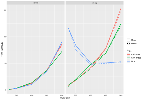
Figure 1: Timing results as the number of predictors is varied with sample size fixed.

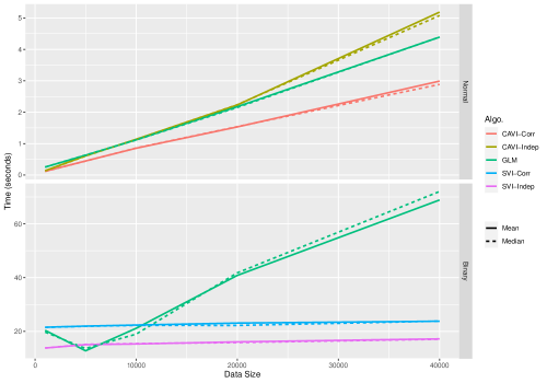
Figure 2: Timing results when the sample size is varied with the number of predictors fixed at 100.

Figure 1 shows our results for the timing experiments when $N$ is fixed and $P$ is varied. For the linear models, we see that the time to convergence increases for each model as the number of predictors is increased. Interestingly, we see that, for the settings considered, our CAVI implementations for normal linear models converge faster than the path algorithm implemented in cv.glmnet(). It can also be seen that assuming an independence structure among the regression coefficients can lead to computational benefits as the number of predictors increases. In the case of the probit regression models, we see, as expected, that the time to convergence for the CAVI algorithms increases with the number of predictors. However, perplexingly, the cv.glmnet() implementation does not seem to increase in computational complexity as the number of predictors increases.

Figure 2 shows the time to convergence when $P$ is fixed and $N$ is varied. We see that in the normal linear model case, our CAVI-Corr implementations continue to outperform cv.glmnet() as the sample size increases. It should be noted that the CAVI-Indep implementation is slower than CAVI-Corr because a large error term needs to be calculated for each predictor in each iteration of the algorithm. In the binary regression cases, the CAVI implementations were substantially slower the glmnet implementations and were omitted from the plot. However, since Bayesian binary regression is an appropriate use case for the SVI algorithm even when the data fits in memory, we see that the use of such algorithms for a fixed batch size and number of iterations done not lead to an increase in computation time as the size of the dataset increases.

7 Discussion

In this chapter we proposed a new R package, vir, for computationally efficient Bayesian linear regression with shrinkage priors. We compared its performance to glmnet, which is one of the most widely used tools for quickly performing variable selection and prediction in linear regression.

We conducted a simulation study which showed that variational algorithms can be relied upon for variable selection and their performance is comparable to MCMC based approaches for parameter estimation and uncertainty quantification in normal linear models. Hence, we have provided a new tool in the Bayesian toolbox for quickly exploring a large number of models before doing a final MCMC based analysis. Second, our timing comparisons showed situations in which our package outperforms state of the art approaches in glmnet, while at the same time providing approximate uncertainty quantification for the coefficients. Additionally, in the normal linear model case, our approach does not require the use of the bootstrap to do uncertainty quantification, which creates substantial computational overhead for frequentist penalization-based approaches to linear regression.

Future work will focus on increasing the number of variational algorithms implemented in our package. At present, we focused on linear and binary regression, and will extend the algorithms to count and survival data. We also aim to add additional methods for clustering with Dirichlet Processes and non-parametric regression models. Finally, while variational algorithms are one way to approximate a posterior distribution for large datasets, our long term goal is to create a package which solves common problems using a variety of methodology for big data analysis in Bayesian models (stochastic gradient MCMC, GPU acceleration, etc.).

References

- Amari (1998) Amari, S.-I. (1998). Natural gradient works efficiently in learning. Neural computation 10, 251–276.
- Bates et al. (2013) Bates, D., Eddelbuettel, D., et al. (2013). Fast and elegant numerical linear algebra using the rcppeigen package. Journal of Statistical Software 52, 1–24.
- Bernardo and Smith (2000) Bernardo, J. M. and Smith, A. F. (2000). Bayesian theory, volume 405. John Wiley & Sons.
- Betancourt (2017) Betancourt, M. (2017). A conceptual introduction to hamiltonian monte carlo. arXiv preprint arXiv:1701.02434 .
- Bishop (2006) Bishop, C. M. (2006). Pattern recognition and machine learning. springer.
- Blei et al. (2017a) Blei, D. M., Kucukelbir, A., and McAuliffe, J. D. (2017a). Variational inference: A review for statisticians. Journal of the American Statistical Association 112, 859–877.
- Blei et al. (2017b) Blei, D. M., Kucukelbir, A., and McAuliffe, J. D. (2017b). Variational inference: A review for statisticians. Journal of the American Statistical Association 112, 859–877.
- Brooks et al. (2011) Brooks, S., Gelman, A., Jones, G., and Meng, X.-L. (2011). Handbook of markov chain monte carlo. CRC press.
- Carbonetto et al. (2012) Carbonetto, P., Stephens, M., et al. (2012). Scalable variational inference for bayesian variable selection in regression, and its accuracy in genetic association studies. Bayesian analysis 7, 73–108.
- Carvalho et al. (2010) Carvalho, C. M., Polson, N. G., and Scott, J. G. (2010). The horseshoe estimator for sparse signals. Biometrika 97, 465–480.
- Chen et al. (2018) Chen, Y.-C., Wang, Y. S., Erosheva, E. A., et al. (2018). On the use of bootstrap with variational inference: Theory, interpretation, and a two-sample test example. The Annals of Applied Statistics 12, 846–876.
- Eddelbuettel and Francois (2011) Eddelbuettel, D. and Francois, R. (2011). Rcpp: Seamless r and c++ integration. Journal of Statistical Software, Articles 40, 1–18.
- Fasano et al. (2019) Fasano, A., Durante, D., and Zanella, G. (2019). Scalable and accurate variational bayes for high-dimensional binary regression models. arXiv pages arXiv–1911.
- Gelfand and Smith (1990) Gelfand, A. E. and Smith, A. F. (1990). Sampling-based approaches to calculating marginal densities. Journal of the American statistical association 85, 398–409.
- Geman and Geman (1984) Geman, S. and Geman, D. (1984). Stochastic relaxation, gibbs distributions, and the bayesian restoration of images. IEEE Transactions on pattern analysis and machine intelligence pages 721–741.
- Guhaniyogi and Dunson (2015) Guhaniyogi, R. and Dunson, D. B. (2015). Bayesian compressed regression. Journal of the American Statistical Association 110, 1500–1514.
- Hastings (1970) Hastings, W. K. (1970). Monte carlo sampling methods using markov chains and their applications.
- Hoffman et al. (2013) Hoffman, M. D., Blei, D. M., Wang, C., and Paisley, J. (2013). Stochastic variational inference. The Journal of Machine Learning Research 14, 1303–1347.
- Hoffman and Gelman (2014) Hoffman, M. D. and Gelman, A. (2014). The no-u-turn sampler: Adaptively setting path lengths in hamiltonian monte carlo. Journal of Machine Learning Research 15, 1593–1623.
- Holmes et al. (2006) Holmes, C. C., Held, L., et al. (2006). Bayesian auxiliary variable models for binary and multinomial regression. Bayesian analysis 1, 145–168.
- Kingma and Ba (2014) Kingma, D. P. and Ba, J. (2014). Adam: A method for stochastic optimization. arXiv preprint arXiv:1412.6980 .
- Kucukelbir et al. (2017) Kucukelbir, A., Tran, D., Ranganath, R., Gelman, A., and Blei, D. M. (2017). Automatic differentiation variational inference. Journal of Machine Learning Research 18, 1–45.
- Kyung et al. (2010) Kyung, M., Gill, J., Ghosh, M., and Casella, G. (2010). Penalized regression, standard errors, and bayesian lassos. Bayesian Analysis 5, 369–411.
- Ma et al. (2015) Ma, Y.-A., Chen, T., and Fox, E. (2015). A complete recipe for stochastic gradient mcmc. In Advances in Neural Information Processing Systems, pages 2917–2925.
- Makalic and Schmidt (2015) Makalic, E. and Schmidt, D. F. (2015). A simple sampler for the horseshoe estimator. IEEE Signal Processing Letters 23, 179–182.
- Metropolis et al. (1953) Metropolis, N., Rosenbluth, A. W., Rosenbluth, M. N., Teller, A. H., and Teller, E. (1953). Equation of state calculations by fast computing machines. The journal of chemical physics 21, 1087–1092.
- Murphy (2012) Murphy, K. P. (2012). Machine learning: a probabilistic perspective. MIT press.
- Park and Casella (2008) Park, T. and Casella, G. (2008). The bayesian lasso. Journal of the American Statistical Association 103, 681–686.
- Plummer et al. (2019) Plummer, M., Stukalov, A., Denwood, M., and Plummer, M. M. (2019). Package ‘rjags’.
- Quiroz et al. (2018) Quiroz, M., Kohn, R., Villani, M., and Tran, M.-N. (2018). Speeding up mcmc by efficient data subsampling. Journal of the American Statistical Association .
- Rand (1971) Rand, W. M. (1971). Objective criteria for the evaluation of clustering methods. Journal of the American Statistical association 66, 846–850.
- Robert and Casella (2013) Robert, C. and Casella, G. (2013). Monte Carlo statistical methods. Springer Science & Business Media.
- Saibaba et al. (2019) Saibaba, A. K., Bardsley, J., Brown, D. A., and Alexanderian, A. (2019). Efficient marginalization-based mcmc methods for hierarchical bayesian inverse problems. SIAM/ASA Journal on Uncertainty Quantification 7, 1105–1131.
- Schaul et al. (2013) Schaul, T., Zhang, S., and LeCun, Y. (2013). No more pesky learning rates. In International Conference on Machine Learning, pages 343–351.
- Scott et al. (2016) Scott, S. L., Blocker, A. W., Bonassi, F. V., Chipman, H. A., George, E. I., and McCulloch, R. E. (2016). Bayes and big data: The consensus monte carlo algorithm. International Journal of Management Science and Engineering Management 11, 78–88.
- Simon et al. (2011) Simon, N., Friedman, J., Hastie, T., and Tibshirani, R. (2011). Regularization paths for cox’s proportional hazards model via coordinate descent. Journal of Statistical Software 39, 1–13.
- Srivastava et al. (2015) Srivastava, S., Cevher, V., Dinh, Q., and Dunson, D. (2015). Wasp: Scalable bayes via barycenters of subset posteriors. In Artificial Intelligence and Statistics, pages 912–920.
- Stan Development Team (2018) Stan Development Team (2018). Rstan: the r interface to stan. r package version 2.17. 3.
- Sturtz et al. (2005) Sturtz, S., Ligges, U., and Gelman, A. E. (2005). R2winbugs: a package for running winbugs from r.
- Terenin et al. (2019) Terenin, A., Dong, S., and Draper, D. (2019). Gpu-accelerated gibbs sampling: a case study of the horseshoe probit model. Statistics and Computing 29, 301–310.
- Terenin et al. (2020) Terenin, A., Simpson, D., and Draper, D. (2020). Asynchronous gibbs sampling. In International Conference on Artificial Intelligence and Statistics, pages 144–154.