A Simple Mathematical Model for the Asymmetry of Time

1 ABSTRACT

A mathematical model is presented for the dynamics of time relative to space. The model design is analogous to a chemical kinetic reaction based on transition state theory which posits the existence of reactants, activated complex, and products. Here, time future is considered to be analogous to reactants, time now to transition state (activated complex) and time past to products. Thus, future, now, and past events are considered to be distinct from one another in the progression of time which flows from future to now to past. The model also incorporates a cyclical reaction (in a quasi-equilibrium state) between time future and time now as well as an irreversible reaction (that is unidirectional and not in equilibrium) from time now to time past. The results from modeling show that modeling time in terms of changes in space can explain the asymmetric nature of time.

2 INTRODUCTION

It is generally accepted that there is an asymmetry to time as reflected in the “arrow of time” [1, 2, 3]. A common example of this asymmetry is that we can remember the past but we cannot remember the future. However, how time’s asymmetry arises is not well understood. Even in Physics, most mathematical expressions work as well for time in the past as for time in the future, and the only mathematical expressions that capture the asymmetry of time are ones based on the second law of thermodynamics where there is an asymmetric increase in entropy. But this concept only shifts the question to: Where in the past did lower entropy arise that causes time’s behavior to be asymmetric? The objective of the study was to create a model that explains the asymmetric behavior of time.

In designing the model, it was important to incorporate the accepted idea that time is intimately related to space. Indeed, the two were merged together into spacetime in Einstein’s Special and General Relativity theories. Moreover, Minkowski immortalized the concept of spacetime via his address called “Space and Time” which was delivered at the 80${}^{\text{th}}$Assembly of German Natural Scientists and Physicians on September 21, 1908. According to these scientists, our understanding of time can only be complete if we study it with reference to spacetime. Thus, we want to understand time’s asymmetry, including past, present and future, with reference to spacetime.

In his recent book [1], “The Order of Time”, Carlo Rovelli states “The distinction between past, present, and future is not an illusion. It is the temporal structure of the world.” The goal was to model dynamics of time by considering past, present and future as distinct from one another. So, in the model, time past ($t_{\text{P}}$), time now ($t_{\text{N}}$) and time future ($t_{\text{F}}$) events are distinct from one another based on differences in their spatial properties. Time is modeled here as a dynamic process that changes as a function of change in space. Thus, in the model, time was considered as a distinct, quantized variable. The rationale for this assumption is four-fold. (i) That changes in time can occur as a function of gravity and velocity [1, 2, 3]. (ii) Moreover, based on recent work [4] on physical theories of quantum gravity, it is possible to derive a minimum meaningful amount of time, about $10^{-44}$ sec, which is termed “Planck time”. (iii) Based on studies of the red shifts of galaxies [5], it appears that red shifts take on discrete (quantized) values, suggesting that the structure of time intervals makes up the fabric of galaxies. (iv) Finally, a recent hypothesis in physics [6] proposes that there is a quantum of time (the chronon), which is a discrete and indivisible unit of time, and that time is not continuous.

In designing the model, the Universe was considered to be made up of events that are in continuous motion and constant interaction, where an event is any change that happens or takes place in both space and time. The terms and direction of time in the model are best understood using concepts from the philosophy of time [7, 8] where essential facts about time are described in terms of events: “First, we think of events as being arrayed in a certain order, where what is happening depends on where we are in that order. Second, we think of events as coming to be and passing away, as undergoing change over, or in, time.”

The model terms (time future, time now, and time past) are used to describe how events are arrayed in an order, and the model’s direction of time (from future to now to past) is used to describe how events come to be and pass away. In the model, the term time now is a point of reference anywhere in the universe where events progress in one direction and time flows from future to past. In this view, some events, termed time future, are happening prior to time now and are coming to be in time now. Other events, termed time past, take place later than after the given point of reference of time now. This process of “becoming” and “passing” is modeled here as being analogous to a chemical reaction whereby the reactants (time future events) are converted to products (time past events) caused by the interaction of a time future event with another event. The change from time future to past occurs as a time now event that happens instantaneously when an interaction of events happens as a result of a change in entropy.

In this view, spacetime dynamics is considered to be analogous to changes in elements that occur in a chemical reaction as described by transition state theory (TST) [9, 10, 11]. TST provides an explanation for how a reaction takes place at the molecular level defined by rates of elementary chemical reactions. In TST, a transition state (also called an activated complex) exists between reactants and products, which is the instantaneous state immediately before formation of the product. TST also assumes that a unique type of chemical equilibrium exists (described by an equilibrium constant K) between reactants and activated transition state complexes. Figure 1A shows how TST models the energy barrier (i.e. energy of activation or $E_{a}$) that reactants have to cross to form products, and explains how the rate at which reactants form products relates to the energy landscape. In this way, enthalpy ($\Delta\text{H}$), entropy ($\Delta\text{S}$) and the Gibbs free energy ($\Delta\text{G}$) can be computed for various chemical reactions. The TST concept is applied here to explain the flow of time relative to space (Figure 1B).

3 MODEL ASSUMPTIONS

The model, and the six assumptions on which it is based, are given below. Note that, in the design, the rate constant “$k$” has spatial units of $s^{-1}$ where $s=$ space. Time and space variables in the model do not consider dimensions of time or space, but simply consider time as a dynamic variable of space. Of course, the physical measurement of time depends on changes in space.

1. Time past ($t_{\text{P}}$), time now ($t_{\text{N}}$) & time future ($t_{\text{F}}$) events are distinct from one another.

2. $t_{\text{N}}$ is a transition state between $t_{\text{F}}$ and $t_{\text{P}}$ in the progression of $t_{\text{F}}$ to $t_{\text{P}}$ (Note that this is a different view from the common notion of the arrow of time which is held to flow from past to future).
   Namely, time future ($t_{\text{F}}$) progresses to time now ($t_{\text{N}}$) which progresses to time past ($t_{\text{P}}$).

3. There is no $t_{\text{F}}$ without $t_{\text{N}}$, This is modeled as self-renewal of $t_{\text{N}}$ in the generation of $t_{\text{F}}$ based on the rate constant $k_{\text{1}}$.

   $$t_{N}\xlongrightarrow{k_{1}}t_{N}+\text{$t_{\text{F}}$}$$

4. $t_{\text{N}}$ arises from $t_{\text{F}}$, This is modeled as self-renewal of $t_{\text{F}}$ in the generation of $t_{\text{N}}$ based on the rate constant $k_{\text{2}}$

   $$\text{$t_{\text{F}}$}\xlongrightarrow{k_{2}}\text{$t_{\text{F}}$}+t_{N}$$

5. $t_{\text{P}}$ arises from $t_{\text{N}}$. This is modeled as an irreversible reaction from $t_{\text{N}}$ to $t_{\text{P}}$ based on the rate constant $k_{\text{3}}$

   $$t_{N}\xlongrightarrow{k_{3}}\text{$t_{\text{P}}$}$$

6. Time is measured as a sequence of events where time changes ($dt$) as a function of changes in space ($ds$).Time & space are entities expressed in terms of units of time and space.

   $$\frac{\text{$d\text{$t_{\text{F}}$}$}}{\text{$ds$}} =k_{1}\text{$t_{\text{N}}$}$$

   $$\frac{\text{$d\text{$t_{\text{N}}$}$}}{\text{$ds$}} =k_{2}\text{$t_{\text{F}}$}-k_{3}\text{$t_{\text{N}}$}$$

   $$\frac{\text{$d\text{$t_{\text{P}}$}$}}{\text{$ds$}} =k_{3}\text{$t_{\text{N}}$}.$$

4 RESULTS

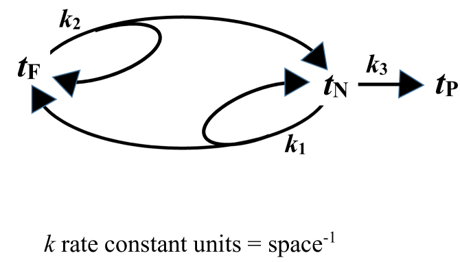
Figure 2: Model design.

Model Design. The model design (Figure 2) was created based on the above assumptions. It incorporates features of cyclical, self-renewal and linear properties of time. The linear feature is consistent with the common notion of an arrow of time that flows in a single direction. However, when time is considered as a kinetic reaction, time progresses from $t_{\text{F}}$ to $t_{\text{N}}$ to $t_{\text{P}}$, which is a different view than the one in classical and modern physics (and Western world cultures) in which time flows from past to present to future. The cyclical feature of time is consistent with beliefs in many Eastern cultures and religions (e.g., the wheel of time) that time is cyclical and quantized [1]. Indeed there are many examples of rhythms, periodicities and cyclical patterns in nature and in biology such as the cycle of birth, life and death, the day/night cycle, and the oscillation of cesium atoms (in atomic clocks). Moreover, there are several cosmological models in which it is proposed that the Universe and time follow infinite or indefinite self-sustaining cycles [1]. Additionally, the cyclical property of the model design is consistent with the idea that an equilibrium exists, based on the use of TST concepts, between $t_{\text{F}}$ and $t_{\text{N}}$ (i.e., equilibrium constant $K_{\text{eq}}=\frac{\text{$t_{\text{N}}$}}{\text{$t_{\text{F}}$}}=\frac{k_{1}}{k_{2}}$). The self-renewal property in the design is consistent with the notion that future and present time always exist and are endless. Self-renewal is not a term (or concept) used very often in physics, but in that field many mechanisms describe oscillatory behavior of elementary particles which resemble self-renewal mechanism. Nonetheless, in biology, self-renewal is a well-understood mechanism that explains the renewal of various living systems.

Transition State Probabilities. Based on the model design, the probability that time now ($t_{\text{N}}$) will transition to time past ($t_{\text{P}}$) or to time future ($t_{\text{F}}$) can be computed as follows:

$$P_{\text{$t_{\text{N}}$}\to\text{$t_{\text{F}}$}} =\frac{k_{1}}{k_{1}+k_{3}}$$

$$P_{\text{$t_{\text{N}}$}\to\text{$t_{\text{P}}$}} =\frac{k_{3}}{k_{1}+k_{3}}$$

In TST (Figure 1A), a similar probability is modeled whereby the activated complex will transition to either the reactant or to the product. Anything that stabilizes the activated complex will increase the probability of its transition to the product [9, 10, 11]. This state is reminiscent of the wave function in quantum mechanics. The probabilities in the wave function represent possible results for measurements made on the system. Wave function collapse occurs when a wave function, initially in superposition of several eigenstates, reduces to a single eigenstate by observation. While the model (Figure 1B) is not intended to relate to quantum mechanics, it is interesting that the dynamics of the transition state (representing $t_{\text{N}}$) consists of a probabilistic state between transition to reactants ($t_{\text{F}}$) vs. products ($t_{\text{P}}$) based on the equations above. Also, according to the model, there are two possible paths to time past, one directly from $t_{\text{N}}$ to $t_{\text{P}}$, and the other from $t_{\text{N}}$ to $t_{\text{F}}$ to $t_{\text{N}}$ to $t_{\text{P}}$. Thus, although this is quite speculative, it could be predicted, based on the model, that there are two possible outcomes for events in time past depending upon the theoretical spacetime frame of the observer.

The general solution. The general solution (see Supplemental material) to the system provides expressions for three eigenvalues ($\lambda_{\text{1,2,3}}$). One eigenvalue ($\lambda_{\text{1}}$) is zero and the others are negative ($\lambda_{\text{2}}$) and positive ($\lambda_{\text{3}}$).

$$\lambda_{1}=0,\,\,\lambda_{2}=\frac{-k_{3}-\sqrt{k_{3}^{2}+4k_{1}k_{2}}}{2}\,\,\,\,\,\,\text{and}\,\,\,\,\,\,\lambda_{3}=\frac{-k_{3}+\sqrt{k_{3}^{2}+4k_{1}k_{2}}}{2}$$

Given “initial conditions” at $s=s_{0}$

$$t_{F}(s_{0})=t_{F,0}\,\,\,\,\,t_{N}(s_{0})=t_{N,0}\,\,\,\,\,\,\text{and}\,\,\,\,\,\,t_{P}(s_{0})=t_{P,0},$$

the constants are determined as

$$c_{1}=\frac{k_{1}\text{$t_{\text{P,0}}$}-k_{3}t_{F,0}}{k_{1}},\,\,\,\,c_{2}=\frac{\lambda_{3}t_{F,0}-k_{1}t_{N,0}}{k_{1}(\lambda_{3}-\lambda_{2})},\,\,\,\,c_{3}=\frac{k_{1}t_{N,0}-\lambda_{2}t_{F,0}}{k_{1}(\lambda_{3}-\lambda_{2})}.$$

Based on the model assumptions, the general solution (below) shows that both $t_{\text{N}}$ and $t_{\text{F}}$ will grow exponentially as long as time zero (0), i.e., either $t_{\text{N}}$($s_{0}$) or $t_{F}$($s_{0}$), or both, is nonzero.

$$t_{F}(s)=\frac{\lambda_{3}t_{F,0}-k_{1}t_{N,0}}{\lambda_{3}-\lambda_{2}}e^{\lambda_{2}(s-s_{0})}+\frac{k_{1}t_{N,0}-\lambda_{2}t_{F,0}}{\lambda_{3}-\lambda_{2}}e^{\lambda_{3}(s-s_{0})}$$

$$t_{N}(s)=\frac{\lambda_{3}t_{F,0}-k_{1}t_{N,0}}{\lambda_{3}-\lambda_{2}}e^{\lambda_{2}(s-s_{0})}+\frac{k_{1}t_{N,0}-\lambda_{2}t_{F,0}}{\lambda_{3}-\lambda_{2}}e^{\lambda_{3}(s-s_{0})}$$

$$\begin{split}\text{$t_{\text{P}}$}(s)=&\frac{k_{1}\text{$t_{\text{P,0}}$}-k_{3}t_{F,0}}{k_{1}}+\frac{k_{3}(\lambda_{3}t_{F,0}-k_{1}t_{N,0})}{k_{1}(\lambda_{3}-\lambda_{2})}\\ &+\frac{k_{3}(k_{1}t_{N,0}-\lambda_{2}t_{F,0})}{k_{1}(\lambda_{3}-\lambda_{2})}\end{split}$$

This result is interesting because, in physics, both theoretical and physical evidence shows that spacetime and the universe are intrinsically expanding. The cause of the expansion is unknown, but it is postulated [2, 3] to be due to dark energy. Although the model does not contribute much understanding to the nature of the expansion of the universe, it does have an emergent (intrinsic) behavior and the general solution shows that both $t_{\text{N}}$ and $t_{\text{F}}$ will grow exponentially as long as either $t_{\text{N}}$(0) or $t_{\text{F}}$(0), or both, are nonzero.

Display of model output in discrete terms. To understand the dynamics of the model, model output is presented visually (Figure 3), in discrete terms, for the equilibrium between $t_{\text{F}}$ and $t_{\text{N}}$. This output assumes that an equilibrium exists between $t_{\text{F}}$ and $t_{\text{N}}$ (i.e., $K_{\text{eq}}=\frac{\text{$t_{\text{N}}$}}{\text{$t_{\text{F}}$}}=\frac{k_{1}}{k_{2}}$), and it does not include the irreversible progression of $t_{\text{N}}$ to $t_{\text{P}}$. It also assumes that the rate from $t_{\text{F}}$ to $t_{\text{N}}$ is slower than the rate from $t_{\text{N}}$ to $t_{\text{F}}$, which provides an asymmetry for time in the system (i.e., $k_{1}\,>\,k_{2};\,\,K_{\text{eq}}>1$). Based on this temporal asymmetry, whereby there is a spatial delay ($dt$/$ds$) in the progression of $t_{\text{F}}$ to $t_{\text{N}}$ relative to $t_{\text{N}}$ to $t_{\text{F}}$, the model output generates the Fibonacci Sequence of numbers (Figure 3, right column). If the spatial delay is longer, then the p-Fibonacci sequence of numbers is generated.

5 DISCUSSION

That there is an asymmetry to the direction of time is generally well-accepted, but there are few models in physics that explain time’s asymmetry. Consequently, the goal of the study was to develop a new model that explains time’s asymmetric behavior. Toward this objective, the widely held idea that space and time are intimately related in a space-time continuum was incorporated in the model. Additionally, to understand time’s asymmetry with reference to spacetime the model design considered past, present and future events as distinct from one another. In this design, time past ($t_{\text{P}}$), time now ($t_{\text{N}}$) and time future ($t_{\text{F}}$) were distinct from one another based on differences in their characteristics relative to space. Time was taken to be a distinct, quantized variable and modeled as a kinetic process that changes as a function of changes in space. In this view, spacetime dynamics were considered to be analogous to changes in elements that occur in a “chemical” kinetic reaction as described by TST. This theory was then applied to explain the flow of time relative to space.

The application of TST to the model yields a concept of the direction of time that is different than the one commonly held in physics in which the present (“now”) is thought to arise out of time past. The notion that time flows from future to present to past is not new. For example, as early as the fourth century, the philosopher Iamblichus spoke of the flow of time from future to present to past [7]. Also, in the book entitled “History of Eternity” [12], Borges states that “It [time] is commonly held to flow from past to future, but the opposite notion… is no less logical. Both are equally probable and equally unverifiable.

The concept of the flow of time as a process is similar to ones found in chemistry, which view chemical reactions as a continuous process involving a gradual transition from reactants to products. In this view, $t_{\text{F}}$ progresses as a continuous process from $t_{\text{F}}$ to $t_{\text{P}}$ with $t_{\text{N}}$ being a transition state. According to TST, a quasi-equilibrium exists between the reactants and the activated complex, which, when applied to the model, corresponds to an equilibrium between $t_{\text{F}}$ and $t_{\text{N}}$. According to TST, the transition state has properties of both reactants and products. Thus, based on reasoning from TST, a time now event would theoretically have properties of both time future and tine past events.

Additionally, in TST, reactants need to have a sufficient energy of activation (Ea) to cross the energy barrier to form products (Figure 1A). Thus, TST provides a mechanism, based on the energy landscape, which explains the rate at which reactants form products. In modeling time here, it is theorized that the interaction of time now events needs to create a sufficiently low level of entropy to increase the potential (available) entropy to cross the transition state (time now) barrier to progress to form time past events (Figure 1B). Also, if an equilibrium does exist between $t_{\text{F}}$ and $t_{\text{N}}$, there would theoretically be a reversal of time, i.e. in the reverse reaction $t_{\text{N}}$ to $t_{\text{F}}$.

Furthermore, in TST, factors that stabilize the transition state will lower the peak of the activation energy curve (Figure 4A). That is, the higher the energy of activation the slower the rate of reaction and vice versa. Thus, factors that stabilize the activation complex (e.g. catalysis by enzymes) will lower the Ea and increase the rate of the reaction. Thus, in modeling time (Figure 4B), it is conjectured that the effect of gravity could raise the peak of the curve, which would delay progression of $t_{\text{F}}$ to $t_{\text{P}}$, and slow time down.

If equilibrium is modeled as a reversible reaction between $t_{\text{N}}$ and $t_{\text{F}}$, but does not include the self-renewal mechanisms for $t_{\text{N}}$ and $t_{\text{F}}$, it would require the assumption that there is an excess of $t_{\text{F}}$ or an endless amount of $t_{\text{F}}$. In the latter case, a large amount of $t_{\text{F}}$ would theoretically have to be produced at the beginning of the universe through a mechanism such as the singularity of a big bang. The model does not address events such as the beginning of time or of the Universe that might have occurred. It was designed mainly to explain the asymmetry of time.

So how does the model simulate the asymmetric nature of time whereby the flow of time occurs in a single direction? The answer is that when the progression of time is modeled like “chemical” reaction (whereby $t_{\text{F}}$ is analogous to reactants, $t_{\text{N}}$ to transition state, and $t_{\text{P}}$ to products), time progresses asymmetrically. There are two components to this asymmetry, i). If, based on reasoning from TST, an equilibrium exists between $t_{\text{N}}$ and $t_{\text{F}}$, any difference in the rates of forward and reverse reactions ($k_{\text{1}}$ vs. $k_{\text{2}}$) generates an asymmetry in the dynamics of time. ii). An irreversible reaction from $t_{\text{N}}$ to $t_{\text{P}}$ produces a unidirectional aspect of time flow.

The next question is: What is the possible source of $t_{\text{F}}$ as a “reactant” species? The model does not answer this question, but the general solution does indicate that $t_{\text{F}}$ is not initially zero. The self-renewing property of time in the model in which $t_{\text{N}}$ and $t_{\text{F}}$ inter-convert and self-renew, simulates the persistent nature of future and present time. Indeed, time appears to be endless and continuously renewing in the Universe. Self-renewal is also consistent with the equilibrium concept in TST in which $t_{\text{F}}$ and $t_{\text{N}}$ are in equilibrium in the application of this theory to the model.

In conclusion, the model of time presented here simulates the self-renewal, cyclic and linear properties of spacetime. By studying the difference between $k_{\text{1}}$ and $k_{\text{2}}$, the model might also help us determine what changes in spacetime could account for the effects of gravity and velocity on the flow of time. Thus, the results from the study not only show that modeling time in terms of changes in space can explain the asymmetric (and cyclic) nature of time, but also, they indicate that time is self-renewing and grows exponentially.

6 ACKNOWLEDGEMENTS:

I want to express sincere gratitude to my close colleagues Drs Gilberto Schleiniger and Jeremy Fields for their extremely helpful input and assistance with the writing of this manuscript.

7 FIGURE LEGENDS:

Figure 1. Model of $t_{\text{N}}$ as a transition state. Panel A shows the classic diagram from transition state theory for the sequence of a chemical reaction. In this concept, the progress of the reaction is from reactants to transition state to products. The transition state (activated complex) is an instantaneous point in the conversion of the initial state into the final state, which can be used to model any process that occurs at a finite rate. In the TST, it is assumed that an equilibrium exists between the reactants and the transition state activated complex. Panel B shows the progression of time based on the concepts of transition state theory. In this view, time progresses as a process or a reaction from $t_{\text{F}}$ to $t_{\text{N}}$ to $t_{\text{P}}$. And, $t_{\text{N}}$ is considered to be the momentary transition state between $t_{\text{F}}$ and $t_{\text{P}}$. The reaction from $t_{\text{N}}$ to $t_{\text{N}}$ is considered to be irreversible.

Figure 2. Model design. The model design in this figure incorporates features of cyclical, self-renewal and linear properties of time. The linear feature is consistent with the common notion of an arrow of time that flows in a single direction. It is important to note, however, when time is considered as a reaction, time progresses from $t_{\text{F}}$ to $t_{\text{N}}$ to $t_{\text{P}}$, which is in contrast to the view in classical and modern Physics (and Western world cultures) that time flows from past to present to future. Additionally, the cyclical property of the model design is consistent with the idea that an equilibrium exists, based on TST concepts, between $t_{\text{N}}$ and $t_{\text{F}}$. The self-renewal property in the design is consistent with the notion that future and present time always exist and are endless.

Figure 3. Discrete model for the evolution of time in space. This model is based on the assumption that there is an equilibrium between $t_{\text{F}}$ and $t_{\text{N}}$ and it does not include the irreversible progression of $t_{\text{N}}$ to $t_{\text{P}}$. It also assumes that the rate from $t_{\text{F}}$ to $t_{\text{N}}$ is slower than the rate from $t_{\text{N}}$ to $t_{\text{F}}$, which provides an asymmetry for time in the system (i.e., $k_{1}>k_{2}$). Based on this asymmetry, whereby there is a spatial delay ($dt$/$ds$) in the progression of $t_{\text{F}}$ to $t_{\text{N}}$ relative to $t_{\text{N}}$ to $t_{\text{F}}$, the model output generates the Fibonacci Sequence of numbers. If the spatial delay is longer, then the p-Fibonacci sequence of number is generated.

Figure 4. Model of $t_{\text{N}}$ as a transition state. Panel A shows, based on transition state theory, how factors that stabilize the transition state effect the peak of the activation energy curve. That is, the higher the energy of activation the slower the rate of reaction and vice versa. Thus, factors that stabilize the activation complex (e.g. catalysis by enzymes) will lower the Ea and increase the rate of the reaction. Panel B shows the progression of time based on the concepts of transition state theory and how gravity could affect the peak of the curve. In the model, it is conjectured that an increase in gravity could raise the peak of the curve, which would delay progression of $t_{\text{F}}$ to $t_{\text{P}}$, and slow time down.

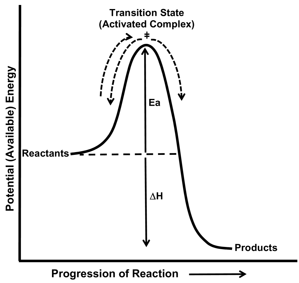
Figure 1A: Model of $t_{\text{N}}$ as a transition state. Panel A.

Figure 1B: Model of $t_{\text{N}}$ as a transition state. Panel B.

Figure 3: Discrete model for the evolution of time in space.

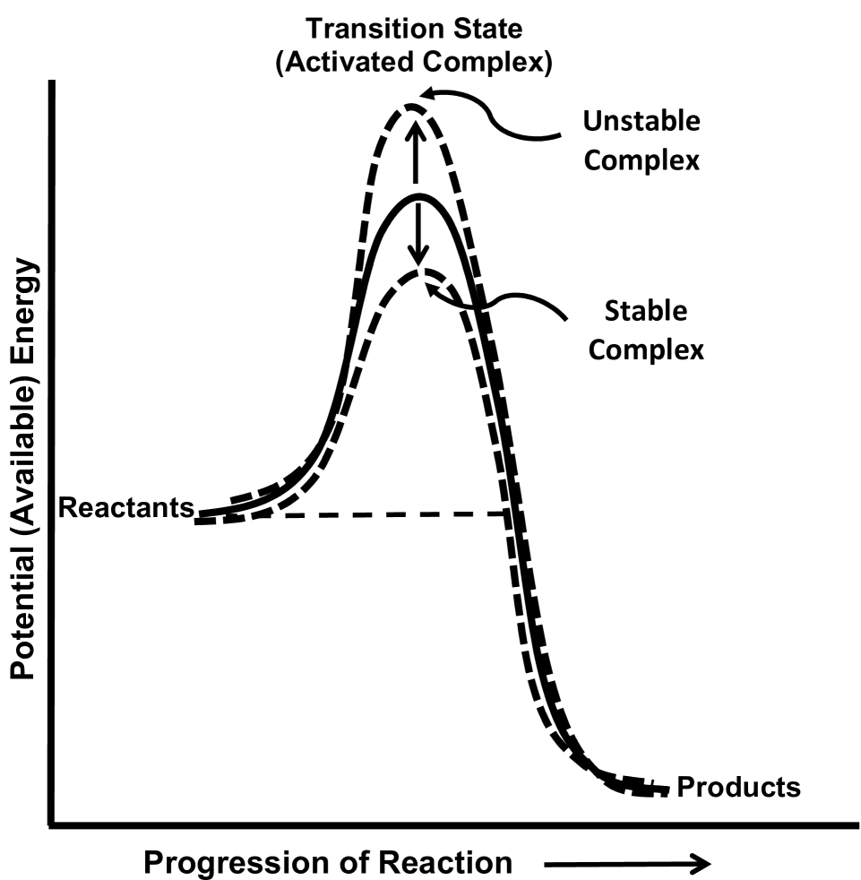
Figure 4A: Model of $t_{\text{N}}$ as a transition state. Panel A.

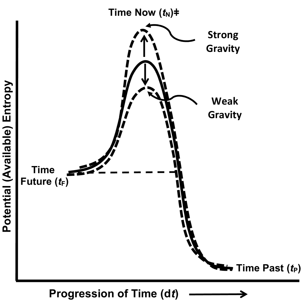
Figure 4B: Model of $t_{\text{N}}$ as a transition state. Panel B.

8 Supplemental Materials

The system of ordinary differential equations (ODEs) is ($\text{$k_{\text{j}}$}>0,\,j\,=\,1,\,2,\,3$)

$$\frac{\text{$d\text{$t_{\text{F}}$}$}}{\text{$ds$}}=k_{1}t_{N}$$ (1)

$$\frac{\text{$dt_{N}$}}{\text{$ds$}}=k_{2}\text{$t_{\text{F}}$}-k_{3}t_{N}$$ (2)

$$\frac{\text{$d\text{$t_{\text{P}}$}$}}{\text{$ds$}}=k_{3}t_{N}.$$ (3)

This system can be written in vector form as follows.

$$\frac{\text{$d\textbf{t}$}}{\text{$ds$}}=A\textbf{t},$$ (4)

where

$$\text{{t}}=\begin{pmatrix}t_{F}\\ t_{N}\\ t_{P}\end{pmatrix},\,\,\,\,\,\,\text{and}\,\,\,\,\,\,\text{{A}}=\begin{pmatrix}0&k_{1}&0\\ k_{2}&-k_{3}&0\\ 0&k_{3}&0\end{pmatrix}.$$

The eigenvalues of the system satisfy

$$\text{det}(\lambda\text{{I - A}})=0,\,\text{i.e}\,\,\begin{vmatrix}\lambda&-k_{1}&0\\ -k_{2}&\lambda+k_{3}&0\\ 0&-k_{3}&\lambda\end{vmatrix}=\lambda^{2}(\lambda+k_{3})-k_{1}k_{2}\lambda=0.$$

Hence, the eigenvalues satisfy $\lambda(\lambda^{2}+k_{3}\lambda-k_{1}k_{2})=0$ and they are

$$\lambda_{1}=0,\,\,\lambda_{2}=\frac{-k_{3}-\sqrt{k_{3}^{2}+4k_{1}k_{2}}}{2}\,\,\,\,\,\,\text{and}\,\,\,\,\,\,\lambda_{3}=\frac{-k_{3}+\sqrt{k_{3}^{2}+4k_{1}k_{2}}}{2}$$ (5)

Therefore, there is one zero eigenvalue ($\lambda_{\text{1}}$), one negative eigenvalue ($\lambda_{\text{2}}$), and one positive eigenvalue ($\lambda_{\text{3}}$). The corresponding eigenvectors are calculated below.

• For $\lambda_{\text{1}}$ = 0:

  $$V_{1}=\begin{pmatrix}0\\ 0\\ 1\\ \end{pmatrix}$$

• For $\lambda_{\text{1, 2}}$ = $\frac{-k_{3}\pm\sqrt{k_{3}^{2}+4k_{1}k_{2}}}{2}$:

  $$V_{2}=\begin{pmatrix}k_{1}\\ \lambda_{2}\\ k_{3}\\ \end{pmatrix}\,\,\,\,\,\,\text{and}\,\,\,\,\,\,V_{3}=\begin{pmatrix}k_{1}\\ \lambda_{3}\\ k_{3}\end{pmatrix}.$$

  
  

The general solution of the system of ODEs (4) is

$$\text{t}=c_{1}V_{1}+c_{2}e^{\lambda_{2}(s-s_{0})V_{2}}+c_{3}e^{\lambda_{3}(s-s_{0})}V_{3}.$$ (6)

Given “initial conditions” at $s=s_{0}$

$$t_{F}(s_{0})=t_{F,0}\,\,\,\,\,t_{N}(s_{0})=t_{N,0}\,\,\,\,\,\,\text{and}\,\,\,\,\,\,t_{P}(s_{0})=t_{P,0},$$ (7)

the constants are determined as

$$c_{1}=\frac{k_{1}t_{P,0}-k_{3}t_{F,0}}{k_{1}},\,\,\,\,\,c_{2}=\frac{\lambda_{3}t_{F,0}-k_{1}t_{N,0}}{k_{1}(\lambda_{3}-\lambda_{2})},\,\,\,\,\,c_{3}=\frac{k_{1}t_{N,0}-\lambda_{2}t_{F,0}}{k_{1}(\lambda_{3}-\lambda_{2})}.$$

Thus, the solution to the initial-value problem (1)–(3), (7) is

$$t_{F}(s)=\frac{\lambda_{3}t_{F,0}-k_{1}t_{N,0}}{\lambda_{3}-\lambda_{2}}e^{\lambda_{2}(s-s_{0})}+\frac{k_{1}t_{N,0}-\lambda_{2}t_{F,0}}{\lambda_{3}-\lambda_{2}}e^{\lambda_{3}(s-s_{0})}$$ (8)

$$t_{N}(s)=\frac{\lambda_{3}t_{F,0}-k_{1}t_{N,0}}{\lambda_{3}-\lambda_{2}}e^{\lambda_{2}(s-s_{0})}+\frac{k_{1}t_{N,0}-\lambda_{2}t_{F,0}}{\lambda_{3}-\lambda_{2}}e^{\lambda_{3}(s-s_{0})}$$ (9)

$$\begin{split}\text{$t_{\text{P}}$}(s)=&\frac{k_{1}\text{$t_{\text{P,0}}$}-k_{3}t_{F,0}}{k_{1}}+\frac{k_{3}(\lambda_{3}t_{F,0}-k_{1}t_{N,0})}{k_{1}(\lambda_{3}-\lambda_{2})}\\ &+\frac{k_{3}(k_{1}t_{N,0}-\lambda_{2}t_{F,0})}{k_{1}(\lambda_{3}-\lambda_{2})}\end{split}$$ (10)

where $\lambda_{j},\,\,j=2,\,3$, are given in (5).

References

- [1] Rovielli C (2018) The Order of Time, (Riverhead Books, New York).
- [2] Davies P (1995) About Time: Einstein’s Unfinished Revolution, (Simon & Schuster, New York).
- [3] Muller RA (2016) Now: The Physics of Time, (WW Norton & Company, New York & London).
- [4] Planck Time: Wikipedia (2018) https://en.wikipedia.org/wiki/Planck_time.
- [5] Redshift quantization – Wikipedia (2018), http://en.wikipedia.org/wiki/Redshift_quantization.
- [6] Chronon – Wikipedia (2018) https://en.wikipedia.org/wiki/Chronon.
- [7] Bardon A (2013) A Brief History of the Philosophy of Time, (Oxford University Press, New York).
- [8] Reichembach (1956) The Direction of Time, ( Dover Publications Inc, Mineola, New York).
- [9] Beynon JH and Gilbert JR (1984) Application of Transition State Theory to Unimolecular Reactions: An Introduction, (John Wiley & Sons, New York).
- [10] Glasstone S, Laidler KJ, Eyring H (1941) The Theory of Rate Processes: The Kinetics of Chemical Reactions, Viscosity, Diffusion and Electrochemical Phenomena, (McGraw-Hill Book Company Inc, New York & London).
- [11] Transition state theory – Wikipedia (2018), https://en.wikipedia.org/wiki/Transition_state_theory
- [12] Borges JL (1936) History of Eternity, (Viau y Zona, Buenos Aires).