Entropy production and entropy extraction rates for a Brownian particle that walks in underdamped medium

Abstract

The expressions for entropy production, free energy, and entropy extraction rates are derived for a Brownian particle that walks in an underdamped medium. Our analysis indicates that as long as the system is driven out of equilibrium, it constantly produces entropy at the same time it extracts entropy out of the system. At steady state, the rate of entropy production ${\dot{e}}_{p}$ balances the rate of entropy extraction ${\dot{h}}_{d}$. At equilibrium both entropy production and extraction rates become zero. The entropy production and entropy extraction rates are also sensitive to time. As time progresses, both entropy production and extraction rates increase in time and saturate to constant values. Moreover employing microscopic stochastic approach, several thermodynamic relations for different model systems are explored analytically and via numerical simulations by considering a Brownian particle that moves in overdamped medium. Our analysis indicates that the results obtained for underdamped cases quantitatively agree with overdamped cases at steady state. The fluctuation theorem is also discussed in detailed.

I Introduction

Exploring the thermodynamic feature of equilibrium systems is vital and recently have received significant attentions since these systems serve as a starting point to study the thermodynamic properties of systems which are far from equilibrium. Because most physically relevant systems are far from equilibrium, it is vital to explore the thermodynamic properties of systems which are driven out of equilibrium. However such systems are often challenging since their thermodynamic relations such as entropy and free energy depend on their reaction rates. Despite the challenge, the thermodynamic relations of systems which are far from equilibrium are explored in the works mu1 ; mu2 ; mu3 ; mu4 . Particularly, the Boltzmann-Gibbs nonequilibrium entropy along with the entropy balance equation serves as an important tool to explore the nonequilibrium thermodynamic features mu1 ; mu2 ; mu3 .

In the past, microscopic stochastic approach has been used by Schnakenberg to derive various thermodynamic quantities such as entropy production rate in terms of local probability density and transition probability rate mu3 . Later, many theoretical studies were conducted see for example the works mu4 ; mu5 ; mu6 ; mu7 ; mu8 ; mu9 ; mu10 ; mu11 ; mu12 ; mu13 ; mu14 ; mu15 ; mu16 . Recently, we presented an exactly solvable model and studied the factors that affect the entropy production and extraction rates mu17 ; muu17 ; muuu17 for a Brownian particle that walks on discrete lattice system. More recently, using Boltzmann-Gibbs nonequilibrium entropy, we derived the general expressions for the free energy, entropy production and entropy extraction rates for a Brownian particle moving in a viscous medium where the dynamics of its motion is governed by the Langevin equation. Employing Boltzmann-Gibbs nonequilibrium entropy as well as from the knowledge of local probability density and particle current, it is shown that as long as the system is far from equilibrium, it constantly produces entropy and at the same time extracts entropy out of the system. Since many biological problems such as intracellular transport of kinesin or dynein inside the cell can be studied by considering a simplified model of particles walking on lattice as discussed in works by T. Bameta $et$. $al$. mu28 , D. Oriola $et$. $al$. mu29 and O. Campas $et$. $al$. mu30 , the model considered will serve as a starting point to study the thermodynamics features of two or more interacting particles hopping on a lattice. At this point, it is important to stress that most of our studies are focused on exploring the thermodynamic property of systems that operate in the classical regimes. For systems that operate at quantum realm, the dependence of thermodynamic quantities on the model parameters is studied in the works mu25 ; mu26 ; mu27 . Particularly, Boukobza. $et$. $al.$ investigated the thermodynamic feature of a three-level maser. Not only the entropy production rate is defined in terms of the system parameters but it is shown that the first and second laws of thermodynamics are always satisfied in the model system mu27 .

In this work, using Langevin equation and Boltzmann-Gibbs nonequilibrium entropy, the general expressions for the free energy, entropy production ${\dot{e}}_{p}$ and entropy extraction rates ${\dot{h}}_{d}$ are derived in terms of velocity and probability distribution considering a Brownian particle that moves in underdamped medium. It is shown that the entropy production and extraction rates increase in time and saturate to a constant value. At steady state, the rate of entropy production balances the rate of entropy extraction while at equilibrium both entropy production and extraction rates become zero. Moreover, after extending the results obtained by Tome. $et.$ $al.$ ta1 to a spatially varying temperature case, we further analyze our model systems. Once again, we show that the entropy production rate ${\dot{e}}_{p}$ increases in time and at steady state (in the presence of load), ${\dot{e}}_{p}={\dot{h}}_{d}>0$. At stationary state (in the absence of load), ${\dot{e}}_{p}={\dot{h}}_{d}=0$. Moreover, when the particle hops in nonisothermal medium where the medium temperature linearly decreasing (in the presence of load), the exact analytic results exhibit that the velocity approach zero when the load approach zero and as long as a periodic boundary condition is imposed. We also show that the approximation performed based on Tome. $et.$ $al.$ ta1 and our general analytic expression agree quantitively. The analytic results also justified via numerical simulations.

Furthermore, we discuss the non-equilibrium thermodynamic features of a Brownian particle that hops in a ratchet potential where the potential is coupled with a spatially varying temperature. It is shown that the operational regime of such Brownian heat engine is dictated by the magnitude of the external load $f$. The steady state current or equivalently the velocity of the engine is positive when $f$ is smaller and the engine acts as a heat engine. In this regime ${\dot{e}}_{p}={\dot{h}}_{d}>0$. When $f$ increases, the velocity of the particle decreases and at stall force, we find that ${\dot{e}}_{p}={\dot{h}}_{d}=0$ showing that the system is reversible at this particular choice of parameter. For large load, the current is negative and the engine acts as a refrigerator. In this region ${\dot{e}}_{p}={\dot{h}}_{d}>0$. Here we first study the underdamped case via simulations and then for overdamped case, the thermodynamic feature for the model system is explored analytically.

The rest of paper is organized as follows: in Section II, we present the model system as well as the derivation of entropy production and free energy. In Section III, we explore the dependence for the entropy production, entropy exaction and free energy rates on the system parameters for a Brownian particle that freely diffuses in isothermal underdamped medium. In section IV, the dependence for various thermodynamic quantities on system parameters is explored considering a Brownian particle that undergoes a biased random walk in a spatially varying thermal arrangement in the presence of external load. In section V, we consider a Brownian particle walking in rachet potential. The fluctuation theorem is discussed in section VI. Section VII deals with summary and conclusion.

II Free energy and Entropy production

In the work ta1 , the expressions for entropy production and entropy extraction rates were presented in terms of particle velocity and probability distribution considering underdamped and isothermal medium. For a spatially varying thermal arrangement, next we derive the thermodynamic quantities by considering a single Brownian particle that hops in underdamped medium along the potential $U(x)=U_{s}(x)+fx$ where $U_{s}(x)$ and $f$ are the periodic potential and the external force, respectively.

For a single particle that is arranged to undergo a random walk, the dynamics of the particle is governed by Langevin equation

$$m{dv\over dt}=-\gamma{dx\over dt}-{dU(x)\over dx}+\sqrt{2k_{B}\gamma T(x)}\xi(t).$$ (1)

The Boltzmann constant $k_{B}$ is assumed to be unity. The random noise $\xi(t)$ is assumed to be Gaussian white noise satisfying the relations $\left\langle\xi(t)\right\rangle=0$ and $\left\langle\xi(t)\xi(t^{\prime})\right\rangle=\delta(t-t^{\prime})$. The viscous friction $\gamma$ is assumed to be constant while the temperature $T(x)$ varies along the medium. For underdamped Langevin case neither Ito nor Stratonovich interpretation is needed as discussed by Sancho. $et$ .$at$ am3 and Jayannavar $et$ .$at$ am33 .

For overdamped case, the above Langevin equation can be written as

$$\gamma(x){dx\over dt} = {-\partial U(x)\over\partial x}-{(1-\epsilon)\over\gamma(x)}{\partial\over\partial x}(\gamma(x)T(x))+$$ (2)

$$\sqrt{2k_{B}\gamma(x)T(x)}\xi(t).$$

Here the Ito and Stratonovich interpretations correspond to the case where $\epsilon=1$ and $\epsilon=1/2$, respectively while the case $\epsilon=0$ is called the Hänggi a post-point or transform-form interpretation am1 ; am2 ; am3 .

The Fokker-Plank equation for underdamped case is given by

$${\partial P\over\partial t} = -{\partial(vP)\over\partial x}-{1\over m}{\partial(U^{\prime}(x)P)\over\partial v}+$$ (3)

$${\gamma\over m}{\partial(vP)\over\partial v}+{\gamma T(x)\over m^{2}}{\partial^{2}P\over\partial v^{2}}$$

where $P(x,v,t)$ is the probability of finding the particle at particular position, velocity and time. The Gibbs entropy is given by

$$S(t)=-\int P(x,v,t)\ln P(x,v,t)dxdv.$$ (4)

The entropy production and dissipation rates can be derived via the approach stated in the work mu7 . The derivative of $S$ with time leads to

$${dS(t)\over dt} = -k_{B}\int{\partial P(x,v,t)\over\partial t}\ln[P(x,v,t)]dxdv.$$ (5)

Eq. (5) can be rewritten as

$${dS(t)\over dt} = {\dot{e}}_{p}-{\dot{h}}_{d}$$ (6)

where ${\dot{e}}_{p}$ and ${\dot{h}}_{d}$ are the entropy production and extraction rates.

In order to calculate ${\dot{h}}_{d}$, let us first find the heat dissipation rate ${\dot{H}}_{d}$ via stochastic energetics that discussed in the works am4 ; am5 . Accordingly the energy extraction rate can be written as

$${\dot{H}}_{d} = -\left\langle\left(-\gamma(x){\dot{x}}+\sqrt{2k_{B}\gamma(x)T(x)}\right).{\dot{x}}\right\rangle$$ (7)

$$= -\left\langle m{vdv\over dt}+vU^{\prime}(x)\right\rangle.$$

Once the energy dissipation rate is obtained, based on our previous works mu17 ; muu17 ; muuu17 , the entropy extraction rate ${\dot{h}}_{d}$ then can be found as

$${\dot{h}}_{d} = -\int\left({m{vdv\over dt}+vU^{\prime}(x)\over T(x)}\right)Pdxdv.$$ (8)

At this point we want to stress that Eq. (8) is exact and do not depend on any boundary condition (as it can be seen in the next sections). Since ${dS(t)\over dt}$ and ${\dot{h}}_{d}$ are computable, the entropy production rate can be readily obtained as

$${\dot{e}}_{p} = {dS(t)\over dt}+{\dot{h}}_{d}.$$ (9)

In high friction limit, Eq. (8) converges to

$${\dot{h}}_{d} = -\int\left[J{U^{\prime}(x)\over T(x)}\right]dx$$ (10)

where the probability current

$$J(x,t) = -\left[U^{\prime}(x)P(x,t)+T(x){\partial P(x,t)\over\partial x}\right].$$ (11)

At steady state ${dS(t)\over dt}=0$ which implies that ${\dot{e}}_{p}={\dot{h}}_{d}>0$. For isothermal case, at stationary state (approaching equilibrium), ${\dot{e}}_{p}={\dot{h}}_{d}=0$.

Moreover, for the case where the probability distribution is either periodic or vanishes at the boundary, Tome $et$. $at.$ ta1 derived the expressions for the entropy production and entropy extraction rates for isothermal case. Following their approach, let us rewrite Eq. (3) as

$${\partial P\over\partial t} = k+{\partial J^{\prime}\over\partial v}$$ (12)

where

$$k=v{\partial P\over\partial x}+{1\over m}(U^{\prime}){\partial P\over\partial v}$$ (13)

and

$$J^{\prime}=-{\gamma\over m}vP-{T(x)\over m^{2}}{\partial P\over\partial v}.$$ (14)

The expression $k$ vanishes after imposing a boundary condition. After some algebra one gets

$${\dot{e}}_{p} = -\int{m^{2}J^{\prime 2}\over PT(x)\gamma}dxdv$$ (15)

and

$${\dot{h}}_{d} = -\int{mvJ^{\prime}\over T(x)}dxdv$$ (16)

respectively. In the next sections we show that indeed Eqs. (8) and (16) as well Eqs. (9) and (15) agree as long as a periodic boundary condition is imposed.

In general, since the expressions for ${\dot{S}}(t)$, ${\dot{e}}_{p}(t)$ and ${\dot{h}}_{d}(t)$ can obtained at any time $t$, the analytic expressions for the change in entropy production, heat dissipation and total entropy can be found analytically via

$$\Delta h_{d}(t) = \int_{0}^{t}{\dot{h}}_{d}(t)dt$$

$$\Delta e_{p}(t) = \int_{0}^{t}{\dot{e}}_{p}(t)dt$$

$$\Delta S(t) = \int_{0}^{t}{\dot{S}}(t)dt$$ (17)

where $\Delta S(t)=\Delta e_{p}(t)-\Delta h_{d}(t)$.

Derivation for the free energy — The free energy dissipation rate ${\dot{F}}(t)$ can be expressed in terms of ${\dot{E}}_{p}(t)$ and ${\dot{H}}_{d}(t)$. ${\dot{E}}_{p}(t)$ and ${\dot{H}}_{d}(t)$ are the terms that are associated with ${\dot{e}}_{p}(t)$ and ${\dot{h}}_{d}(t)$. Let us now introduce ${\dot{H}}_{d}(t)$ for the model system we considered. The heat dissipation rate is either given by Eq. (7) (for any cases) or if a periodic boundary condition is imposed, ${\dot{H}}_{d}(t)$ is given by

$${\dot{H}}_{d} = -\int{mvJ^{\prime}dxdv}.$$ (18)

Equation (18) is notably different from Eqs. (8) and (16), due to the the term $T(x)$. On the other hand, the term ${\dot{E}}_{p}$ is related to ${\dot{e}}_{p}$ and it is given by

$${\dot{E}}_{p} = -\int{m^{2}J^{\prime 2}\over P\gamma}dxdv.$$ (19)

The new entropy balance equation

$${dS^{T}(t)\over dt} = {\dot{E}}_{p}-{\dot{H}}_{d}$$ (20)

is associated to Eq. (6) except the term $T(x)$. Once again, because the expressions for ${\dot{S}}^{T}(t)$, ${\dot{E}}_{p}(t)$ and ${\dot{H}}_{d}(t)$ can be obtained as a function of time $t$, the analytic expressions for the change related to the rate of entropy production, heat dissipation and total entropy can be found analytically via

$$\Delta H_{d}(t) = \int_{0}^{t}{\dot{H}}_{d}(t)dt$$

$$\Delta E_{p}(t) = \int_{0}^{t}{\dot{E}}_{p}(t)dt$$

$$\Delta S(t)^{T} = \int_{0}^{t}{\dot{S}}(t)^{T}dt$$ (21)

where $\Delta S(t)^{T}=\Delta E_{p}(t)-\Delta H_{d}(t)$.

On the other hand, the internal energy is given by

$${\dot{E}}_{in}=\int({\dot{K}}+vU^{\prime}_{s}(x))P(x,v,t)dvdx.$$ (22)

where ${\dot{K}}=m{vdv\over dt}$ and $U^{\prime}_{s}$ denote the rate of kinetic and potential energy, respectively. For a Brownian particle that operates due to the spatially varying temperature case, the total work done is then given by

$${\dot{W}} = \int vfP(x,v,t)dvdx.$$ (23)

The first law of thermodynamics can be written as

$${\dot{E}}_{in}=-{\dot{H}}_{d}(t)-{\dot{W}}.$$ (24)

The change in the internal energy reduces to $\Delta E_{in}=-\int_{0}^{t}({\dot{H}}_{d}(t)+{\dot{W}})dt$

As discussed in the work mu17 ; muu17 ; muuu17 , the rate of free energy is given by ${\dot{F}}={\dot{E}}-T{\dot{S}}$ for isothermal case and ${\dot{F}}={\dot{E}}-{\dot{S}}^{T}$ for nonisothermal case where ${\dot{S}}^{T}={\dot{E}}_{p}-{\dot{H}}_{d}$. Hence we write the free energy dissipation rate as

$${\dot{F}} = {\dot{E}}_{in}-{\dot{S}}^{T}$$ (25)

$$= {\dot{E}}_{in}-{\dot{E}}_{p}+{\dot{H}}_{d}.$$

The change in the free energy is given by

$$\Delta F(t) = -\int_{0}^{t}\left({\dot{W}}+{\dot{E}}_{p}(t)\right)dt.$$ (26)

For isothermal case, at quasistatic limit where the velocity approaches zero $v=0$, ${\dot{E}}_{p}(t)=0$ and ${\dot{H}}_{d}(t)=0$ and far from quasistatic limit $E_{p}={\dot{H}}_{d}>0$ which is expected as the particle operates irreversibly.

III Isothermal case

In this section we discuss the thermodynamic properties for a Brownian particle moving freely without any boundary condition in underdamped medium under the influence of a force $f$ in the absence of a potential $U^{\prime}_{s}$. The general expression for the probability distribution $P(v,t)$ is calculated as

$$P(v,t) = {e^{-{m({-(1-e^{-{\gamma t\over m}})f\over\gamma}+v)^{2}\over 2(1-e^{-{2\gamma t\over m}})T}}\sqrt{{m\over(1-e^{-{2\gamma t\over m})}t}}\over\sqrt{2\pi}}.$$ (27)

The average velocity has a form

$$\left\langle v(t)\right\rangle=\left({1-e^{-{\gamma t\over m}}\over\gamma}\right)f.$$ (28)

At steady state ( the long time limit), the velocity approach $v=f/\gamma$ as expected.

III.1 Free particle diffusion

For a Brownian particle that moves in underdamped medium without an external force, $f=0$, next let us explore how the entropy production and extraction rates behave. From now on, whenever we plot any figures, we use the following dimensionless load ${\bar{f}}=fL_{0}/T_{c}$, temperature ${\bar{T}}=T/T_{c}$ where $T_{c}$ is the reference temperature of the isothermal medium. We also introduced dimensionless parameter ${\bar{x}}=x/L_{0}$. Hereafter the bar will be dropped. From now on all the figures in this section will be plotted in terms of the dimensionless parameters.

The expression for the entropy can be readily calculated by substituting Eq. (27) in Eq. (4). Figure 1 exhibits that the entropy $S(t)$ increases with time and saturates to a constant value which agrees with the results shown in the works muu17 ; muuu17 . On the other hand the entropy production and extraction rates explored via Eqs. (6), (8) and (9) (see Fig.2). The plot ${\dot{e}}_{p}(t)$ (red solid line) and ${\dot{h}}_{d}(t)$ (black solid line) as a function of $t$ for parameter choice $\tau=1$ is depicted in Fig. 2. The figure exhibits that ${\dot{e}}_{p}(t)$ decreases as time increases and in long time limit, it approaches its stationary value ${\dot{e}}_{p}(t)=0$. On the other hand ${\dot{h}}_{d}(t)=0$ regardless of $t$. In the limit $t\to\infty$, ${dS(t)\over dt}=0$ since ${\dot{e}}_{p}(t)={\dot{h}}_{d}(t)=0$ in the long time limit.

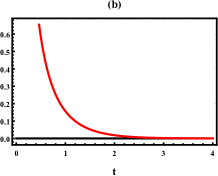
Figure 1: (Color online) (a) The entropy $S(t)$ as a function of $t$ for fixed $\tau=1$. $S(t)$ monotonously increases with $t$ and saturates to a constant value as $t$ further increases. (b) The plot ${\dot{e}}_{p}(t)$ (black solid line) and ${\dot{h}}_{d}(t)$ (red solid line) as a function of $t$ for parameter choice $T=1$. The figure exhibits that ${\dot{e}}_{p}(t)$ decreases as time increases and in the long time limit, it approaches its stationary value ${\dot{e}}_{p}(t)={\dot{h}}_{d}(t)=0$.

III.2 Particle diffusion in the presence of force

In the presence of non-zero force, the particle diffuses under the influence of the external load. Exploiting Eqs. (6), (8) and (9), the dependence of $S(t)$, ${\dot{S}}(t)$, ${\dot{e}}_{p}(t)$ and ${\dot{h}}_{d}(t)$ on model parameters is explored. In Fig. 2a, ${\dot{S}}(t)$ as a function of $t$ is depicted for fixed values of $T=1$ and $f=1.0$. The figure shows that ${\dot{S}}(t)$ monotonously decreases with $t$ and in the limit $t\to\infty$, ${S}(t)$ saturates to zero . Fig. 2b shows the plot ${\dot{e}}_{p}(t)$ as a function of $t$ (red solid lines). In the same figure, the plot of ${\dot{h}}_{d}(t)$ versus $t$ is shown (black solid line). The figure exhibits that in the presence of load, ${\dot{e}}_{p}(t)$ increases as time increases and in long time limit, it approaches its steady state value (see the red solid line). ${\dot{h}}_{d}(t)$ also approaches its steady state value (see the black solid line) and at steady state ${\dot{h}}_{d}(t)={\dot{e}}_{p}(t)>0$. This also indicates that in the presence of symmetry breaking fields such as external force, the system is driven out of equilibrium.

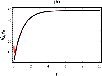
Figure 2: (Color online) (a) The entropy $S(t)$ as a function of $t$ for fixed $\tau=1$. $S(t)$ monotonously increases with $t$ and saturates to a constant value as $t$ further increases. (b) The plot ${\dot{e}}_{p}(t)$ (red solid line) and ${\dot{h}}_{d}(t)$ (black solid line) as a function of $t$ for parameter choice $\tau=1$. The figure exhibits that ${\dot{e}}_{p}(t)$ increases as time increases and in long time limit, it approaches its stationary value ${\dot{e}}_{p}(t)={\dot{h}}_{d}(t)>0$.

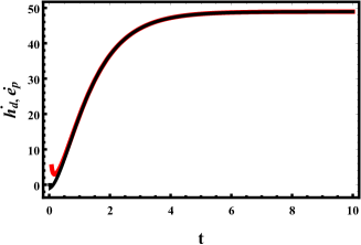
Figure 3: (Color online) The plot ${\dot{e}}_{p}(t)$ (black solid line) and ${\dot{h}}_{d}(t)$ (red solid line) as a function of $t$ for parameter choice $\tau=1$. The figure exhibits that ${\dot{e}}_{p}(t)$ increases as time increases and in long time limit, it approaches its stationary value ${\dot{e}}_{p}(t)={\dot{h}}_{d}(t)>0$.

Even if no periodic boundary condition is imposed, the results shown in Fig. 2 can be also reproduced by employing Eqs. (6), (15) and (16). In fact Fig. 3 is identical to Fig. 2 except that Fig. 3 is plotted via Eqs. (6), (15) and (16) while in plotting Fig. 2, Eqs. (6), (8) and (9) are used. Our analysis also indicates that the free energy dissipation rate ${\dot{F}}$ is always less than zero ${\dot{F}}<0$. As time steps up, it increases with time and approaches zero in the long time limit. All of the results shown in this work also agree with our previous results mu17 ; muu17 ; muuu17 . As before $\Delta h_{d}(t)=h_{d}(t)-h_{d}(t_{0})>0$, $\Delta S(t)=S(t)-S(t_{0})>0$ or $\Delta e_{p}(t)=e_{p}(t)-e_{p}(t_{0})>0$.

IV Nonisothermal case

IV.1 Periodic boundary condition

Now let us consider an important model system where a colloidal particle that undergoes a biased random walk in a spatially varying thermal arrangement in the presence of external load $f$ with no potential. The load is also coupled with a heat bath that decreases from $T_{h}$ at $x=0$ to $T_{c}$ at $x=L_{0}$ along the reaction coordinate in the manner

$$T(x)=\left\{{x(T_{c}-T_{h})\over L_{0}}+T_{h}\right\}.$$ (29)

Here $L_{0}$ denotes the width of the ratchet potential. $T_{h}$ and $T_{c}$ denote the temperature of the hot and cold baths.

Solving Eq. (3) at steady state and imposing a periodic boundary condition, the general expression for the probability distribution is obtained as

$$P(x,v)=e^{-{L_{0}m(f-\gamma v)^{2}\over{2\gamma^{2}L_{0}(L_{0}T_{h}+(T_{c}-T_{h})x)}}}\sqrt{\frac{L_{0}m}{2L_{0}\pi T_{h}+2\pi T_{c}x-2\pi T_{h}x}}.$$ (30)

The average velocity is found to be

$$v={f\over\gamma}.$$ (31)

In the absence of force, the velocity approach zero.

Employing Eqs. (6), (8) and (9), the entropy production and extraction rates are calculated as

$${\dot{h}}_{d}(t) = {\dot{e}}_{p}(t)$$ (32)

$$= {(2fL_{0})^{2}Log[T_{c}/T_{h}]\over{4\gamma L_{0}(T_{c}-T_{h})}}$$

We reproduce the above result (using Tome $et$. $at.$ ta1 approach) via Eqs. (6), (15) and (16) as

$${\dot{h}}_{d}(t) = {\dot{e}}_{p}(t)$$ (33)

$$= {(2fL_{0})^{2}Log[T_{c}/T_{h}]\over{4\gamma L_{0}(T_{c}-T_{h})}}.$$

Surprisingly, in the limit where the load approaches the the stall force, ${\dot{h}}_{d}(t)={\dot{e}}_{p}(t)=0$.

The rate of heat dissipation is calculated using Eq. (7) (or Eq. (18)) and it converges to

$${\dot{H}}_{d}(t) = {\dot{E}}_{p}(t)$$ (34)

$$= {(fL_{0})^{2}\over\gamma L_{0}}.$$

In the limit where the load approach zero, ${\dot{H}}_{d}(t)={\dot{E}}_{p}(t)=0$ showing that at quasistatic limt the system is reversible. On the other hand, the rate of work done is given by

$${\dot{W}}(t) = {\dot{E}}_{p}(t)$$ (35)

$$= {(fL_{0})^{2}\over\gamma L_{0}}.$$

For isothermal case $T_{h}=T_{c}$ one gets $v=f/\gamma$, ${\dot{h}}_{d}(t)={\dot{e}}_{p}(t)=f^{2}L_{0}/\gamma T_{c}$ and ${\dot{H}}_{d}(t)={\dot{E}}_{p}(t)=f^{2}L_{0}/\gamma$.

All of the results shown in this section are justified via numerical simulations by integrating the Langevin equation (1) (employing Brownian dynamics simulation). In the simulation, a Brownian particle is initially situated in one of the potential wells. Then the trajectories for the particle is simulated by considering different time steps $\Delta t$ and time length $t_{max}$. In order to ensure the numerical accuracy $10^{9}$ ensemble averages have been obtained. Fig. 4 depicts the plot $v$ as a function of load $f$. The figure shows the velocity steps up linearly with the load $f$.The simulation results obtained agree with analytic results.

The plot ${\dot{e}}_{p}(t)$ and ${\dot{h}}_{d}(t)$ as a function of $f$ is depicted in Fig. 5a for parameter choice $\tau=2$. The figures show that ${\dot{e}}_{p}(t)$ and ${\dot{h}}_{d}(t)$ have a nonlinear dependence on the load. Figure 5b also exhibits the plot ${\dot{e}}_{p}(t)$ and ${\dot{h}}_{d}(t)$ as a function of $\tau$ for fixed $f=2$. The figure depicts that ${\dot{e}}_{p}(t)$ and ${\dot{h}}_{d}(t)$ decrease as the temperature increases.

Figure 4: (Color online) The plot $v$ as a function of load $f$. The dotted lines are plotted via Brownian dynamic simulation while the solid lines are potted using the analytic Eq. (32).

Figure 5: (Color online) (a) The plot ${\dot{e}}_{p}(t)$ and ${\dot{h}}_{d}(t)$ as a function of $f$ for parameter choice $\tau=2$. (b) The plot ${\dot{e}}_{p}(t)$ and ${\dot{h}}_{d}(t)$ as a function of $\tau$ for parameter choice $f=2$.

IV.2 Nonisothermal case without boundary condition

All the discussed thermodynamic quantities are quite sensitive to the choice of the boundary condition. For instance, when no boundary condition is imposed, we find the velocity for underdamped case as

$$v={2fL_{0}+(T_{c}-T_{h})\over 2\gamma L_{0}}.$$ (36)

showing the particle stalls when

$$f_{s}={(T_{h}-T_{c})\over 2\gamma L_{0}}.$$ (37)

When $f<f_{s}$, the particle velocity $v>0$ and if $f>f_{s}$, the particle velocity $v<0$. At stall force $f=f_{s}$, $v=0$. The entropy production and extraction rates are given as

$${\dot{h}}_{d}(t) = {\dot{e}}_{p}(t)$$ (38)

$$= {(2fL_{0}+T_{c}-T_{h})^{2}Log[T_{c}/T_{h}]\over{4\gamma L_{0}(T_{c}-T_{h})}}$$

while

$${\dot{H}}_{d}(t) = {\dot{E}}_{p}(t)={(2fL_{0}+T_{c}-T_{h})^{2}\over 4\gamma L_{0}}.$$ (39)

Exploiting Eq. (38), one can see that in the limit $f\to f_{s}$, ${\dot{h}}_{d}(t)\to 0$ and ${\dot{e}}_{p}(t)\to 0$. All of these results indicate that in the absence of boundary conditions, most of the thermodynamic quantities have a functional dependence on $\Delta T=Th-T_{c}$ which agrees with the work by Matsuo $et.$. $al.$ mi1 .

V Brownian particle walking in a ratchet potential where the potential is coupled with a spatially varying temperature

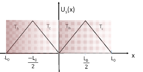
Figure 6: Schematic diagram for a Brownian particle in a piecewise linear potential in the absence of external load. Due to the thermal background kicks, the particle ultimately attains a steady state current (velocity) as long a distinct temperature difference between the hot and the cold reservoirs is retained.

In this section, let us consider a Brownian particle that moves along the potential $U(x)=U_{s}(x)+fx$ where $f$ and $U_{s}(x)$ denote the load and ratchet potential, respectively. The ratchet potential $U_{s}(x)$

$$U_{s}(x)=\left\{\begin{array}[]{cl}2U_{0}[{x\over L_{0}}],&if~{}0<x\leq L_{0}/2;\\ 2U_{0}[{-x\over L_{0}}+1],&if~{}L_{0}/2<x\leq L_{0};\end{array}\right.$$ (40)

is coupled with a heat bath that decreases from $T_{h}$ at $x=0$ to $T_{c}$ at $x=L_{0}$ along the reaction coordinate in the manner

$$T(x)=\left\{{x(T_{c}-T_{h})\over L_{0}}+T_{h}\right\}.$$ (41)

Here $U_{0}$ denots the barrier height. The ratchet potential has a potential maxima at $x=L_{0}/2$ and potential minima at $x=0$ and $x=L_{0}$. The potential profile repeats itself such that $U_{s}(x+L_{0})=U_{s}(x)$. Next let us consider the undrdamped case.

V.1 Underdamped case

Let us now explore the dependence of thermodynamic quantities via numerical simulations by integrating Eq. (1). In Fig. 7a, the plot of $v$ as a function of $U_{0}$ is depicted for fixed $\tau=2$, $f=0.0$, $m=1$ and $\gamma=1$. The figure shows that the velocity peaks at a certain $U_{0}$. On the other hand the plot of $v$ as a function of $U_{0}$ is shown in Fig. 7b for fixed $\tau=2$, $f=0.5$, $m=1$ and $\gamma=1$. The figure shows that the velocity is negative below a certain $U_{0}$. As $U_{0}$ steps up the velocity steps up and attains an optimum value.

Figure 7: (Color online)(a) $v$ as a function of $U_{0}$ for fixed $\tau=2$, $f=0.0$, $m=1$ and $\gamma=1$. (b) $v$ as a function of $U_{0}$ for fixed $\tau=2$, $f=0.5$, $m=1$ and $\gamma=1$.

Figure 8: (Color online)(a) $v$ as a function of $f$ for fixed $\tau=2$, $U_{O}=2.0$ (top) and $U_{O}=1.0$ (bottom), $m=1$ and $\gamma=1$.

The velocity decreases monotonously when the load steps as shown in Fig. 8. At stall force the velocity becomes zero. Further increases in the load leads to a current reversal. The plot ${\dot{e}}_{p}(t)$ and ${\dot{h}}_{d}(t)$ as a function of $U_{0}$ for parameter choice $f=2$ is determined via simulations as shown in Fig. 9.

Figure 9: (Color online) (a) The plot ${\dot{e}}_{p}(t)$ and ${\dot{h}}_{d}(t)$ as a function of $U_{0}$ for parameter choice $\tau=12$ and $f=0.5$. (b) The plot ${\dot{e}}_{p}(t)$ and ${\dot{h}}_{d}(t)$ as a function of $U_{0}$ for parameter choice $f=2.0$ (solid line) and $\tau=2.0$.

V.2 Overdamped case

In the high friction limit, as discussed before, the dynamics of the particle is governed by the Langevin equation

$$\gamma(x){dx\over dt} = -{\partial(U(x)+{T(x)\over 2})\over\partial x}+\sqrt{2k_{B}\gamma(x)T(x)}\xi(t).$$ (42)

The corresponding Fokker Planck equation is given by

$${\partial P(x,t)\over\partial t}={\partial\over\partial x}(U^{\prime}(x)P(x,t)+{T^{\prime}(x)\over 2}P(x,t)+T(x){\partial\over\partial x}P(x,t))$$ (43)

where $P(x,t)$ is the probability density of finding the particle at position x at time t, $U^{\prime}(x)={d\over dx}U$. The current is given by

$$J(x,t) = -\left[U^{\prime}(x)P(x,t)+{T^{\prime}(x)\over 2}P(x,t)+T(x){\partial P(x,t)\over\partial x}\right].$$ (44)

In long time limit, the expression for the constant current, $J$, is given in Appendix A. The change in entropy is given as muuu17

$${dS(t)\over dt} = {\dot{e}}_{p}-{\dot{h}}_{d}$$ (45)

$$= \int{{J^{2}\over P(x,t)T(x)}+J{U^{\prime}(x)\over T(x)}+J{T^{\prime}(x)\over 2T(x)}}dx$$

where the entropy production rate ${\dot{e}}_{p}$ and dissipation rate ${\dot{h}}_{d}$ are given as

$${\dot{e}}_{p} = \int{J^{2}\over P(x,t)T(x)}dx$$ (46)

and

(47)

respectively. Here unlike isothermal case, we have additional term $J{T^{\prime}(x)\over 2T(x)}dx$. At steady state ${dS(t)\over dt}=0$ which implies that ${\dot{e}}_{p}={\dot{h}}_{d}>0$. At stationary state (approaching equilibrium), $J=0$ since detailed balance condition is preserved. Hence ${\dot{e}}_{p}={\dot{h}}_{d}=0$.

In order to relate the free energy dissipation rate with ${\dot{E}}_{p}(t)$ and ${\dot{H}}_{d}(t)$ let us now introduce ${\dot{H}}_{d}(t)$ for the model system we considered. The heat dessipation rate is given by

$${\dot{H}}_{d} = \int\left(JU^{\prime}(x)+{JT^{\prime}(x)\over 2}\right)dx.$$ (48)

${\dot{E}}_{p}$ is the term related to to ${\dot{e}}_{p}$ and it is given by

$${\dot{E}}_{p} = \int\left({J^{2}\over P(x,t)}\right)dx.$$ (49)

We have now a new entropy balance equation

$${dS(t)^{T}\over dt} = {\dot{E}}_{p}-{\dot{H}}_{d}$$ (50)

$$= \int\left({J^{2}\over P(x,t)}+JU^{\prime}(x)+JT^{\prime}(x)\right).$$

Since the analytic expressions for $J(x,t)$ and $P(x,t)$ is given in Appendix A, all of the above expressions are exact but lengthy.

If one considers a periodic boundary condition at steady state in the absence of ratchet potential $U_{0}=0$, the results obtained are quantitatively agree with underdmaped case (Section IV ) and one gets

$${\dot{h}}_{d}(t) = {\dot{e}}_{p}(t)$$ (51)

$$= {(2fL_{0})^{2}Log[T_{c}/T_{h}]\over{4\gamma L_{0}(T_{c}-T_{h})}}$$

and

$${\dot{H}}_{d}(t) = {\dot{E}}_{p}(t)$$ (52)

$$= {(fL_{0})^{2}\over\gamma L_{0}}.$$

The steady state current is zero at stall load

$$f_{s}={2U_{0}\over L}{\ln\left[{4\tau\over(1+\tau)^{2}}\right]\over\ln\left[{1\over\tau}\right]}$$ (53)

which implies the particle velocity $v>0$ when $f<f_{s}$ and at stall force $v=0$. When $f>f_{s}$, $v<0$. In the quasistatic limit $v\to 0$ ($J\to 0$), the system is reversible.

On the contrary, in the absence of any boundary condition, the calculated thermodynamic quantities are quantitatively the same as to result shown in Section IV B. For instance, in the absence of potential, the velocity can be calculated as $v=JL$. Alternatively, we can also find $v$ by taking the time average of Eq. (42) as

$$\gamma v = \left\langle{\partial(fx+{T(x)\over 2})\over\partial x}+\sqrt{2k_{B}\gamma(x)T(x)}\xi(t)\right\rangle$$

$$\gamma v = f+{(T_{h}-T_{c})\over 2L_{0}}$$

$$v = {2fL_{0}+(T_{c}-T_{h})\over 2\gamma L_{0}}.$$ (54)

Eq. (54) is the same as Eq. (36). At this point, we want to stress that at steady state, most of the derived physical quantities are similar both quantitatively and qualitatively whether the particle is in undrdamped or overdamped medium.

Derivation for the free energy — Next assuming a periodic boundary condition where the term $T^{\prime}(x)$ vanishes, let us further explore the model system. The expressions for the work done by the Brownian particle as well as the amount heat taken from the hot bath and the amount of heat given to the cold reservoir can be derived in terms of the stochastic energetics discussed in the works am4 ; am5 . The heat taken from any heat bath can be evaluated via am4 ; am5 ${\dot{Q}}=\left\langle\left(-\gamma(x){\dot{x}}+\sqrt{2k_{B}\gamma(x)T(x)}\right).{\dot{x}}\right\rangle$ while the work done by the Brownian particle against the load is given by ${\dot{W}}=\left\langle f{\dot{x}}\right\rangle.$ We can also find the expression for the input heat $Q_{in}^{s}$ and $W^{s}$ as

$${\dot{Q}}_{in} = \int_{0}^{L_{0}/2}\left(-\gamma(x){\dot{x}}+\sqrt{2k_{B}\gamma(x)T(x)}\right)Jdx$$

$$= \int_{0}^{L_{0}/2}\left[\left({2U_{0}\over L_{0}}\right)+f\right]Jdx$$

$$= U_{0}J+{fL_{0}J\over 2}.$$

Here the integral is evaluated in the interval of $(0,L_{0}/2)$ since the particle has to get a minimal amount of heat input from the heat bath located in the left side of the ratchet potential to surmount the potential barrier. The work done is also given by

$${\dot{W}} = \int_{0}^{L_{0}}fdx=fL_{0}J.$$ (56)

The first law of thermodynamics states that $Q_{in}^{s}-Q_{out}^{s}=W^{s}$ where $Q_{out}^{s}$ is the heat given to the colder heat bath. Thus

$${\dot{Q}}_{out} = {\dot{Q}}_{in}-{\dot{W}}=U_{0}J-{fL_{0}J\over 2}.$$ (57)

The second law of thermodynamics can be rewritten in terms of the housekeeping heat and excess heat. For the model system we consider, when the particle undergoes a cyclic motion, at least it has to get $fLJ$ amount of energy rate from the hot reservoir in order to keep the system at steady state. Hence $fLJ$ is equivalent to the housekeeping heat $Q_{hk}$ and we can rewrite Eq. (25) as

$${\dot{F}}(t)+{\dot{E}}_{p}(t)={\dot{E}}_{in}(t)+{\dot{H}}_{d}(t)=-fLJ=-{\dot{Q}}_{hk}$$ (58)

while the expression for the excess heat ${\dot{Q}}_{ex}$ is given by

$$Q_{ex}={\dot{H}}_{d}-{\dot{Q}}_{hk}.$$ (59)

For isothermal case, we can rewrite the second law of thermodynamics as

$${\dot{S}}^{T}(t)={\dot{E}}_{p}-{\dot{H}}_{d}={-\dot{F}}-{\dot{Q}}_{ex}$$ (60)

and

$${\dot{F}}={\dot{Q}}_{hk}-{\dot{E}}_{p}.$$ (61)

At this point we want to stress that such kind of Brownian motor is inherently irreversible. This can be more appreciated by calculating the efficiency of the engine. The efficiency is given as

$$\eta=W/Q_{in}.$$ (62)

In the quasistatic limit ($J\to 0$), we find

$$\eta=1-{ln\left[{1+\tau\over 2\tau}\right]\over ln\left[{2\over\tau+1}\right]}$$ (63)

which is approximately equal to the efficiency of the endorevesible heat engine $\eta_{CA}$

$$\eta_{CA}=1-\sqrt{1/\tau}$$ (64)

as long as the temperature difference between the hot and the cold reservoirs is not large. In order to appreciate this let us Taylor expand Eqs. (63) and (64) around $\tau=1$ and after some algebra one gets

$$\eta = \eta_{CA}={\tau-1\over 2}-{3\over 8}(\tau-1)^{2}+\ldots$$ (65)

$$= {\eta_{CAR}\over 2}+{\eta_{CAR}^{2}\over 8}+{\eta_{CAR}^{3}\over 96}+\ldots$$

which exhibits that both efficiencies are equivalent in this regime. Here $\eta_{CAR}$ is the Carnot efficiency $\eta_{CAR}=1-1/\tau$.

Next we study how the rate of entropy production ${\dot{e}}_{p}(t)$ and the rate of entropy extraction ${\dot{h}}_{d}(t)$ behave. The plot of ${\dot{e}}_{p}(t)$ and ${\dot{h}}_{d}(t)$ as a function of $f$ is depicted in Fig. 10a for fixed values of $U_{0}=2.0$ and $\tau=12.0$. The plot ${\dot{e}}_{p}(t)$ and ${\dot{h}}_{d}(t)$ as a function of $\tau$ is depicted for parameter choice $f=2.0$ (solid line) and $U_{0}=2.0$. Figure 10b indicates that far from steady state ${\dot{e}}_{p}(t)>0$ and ${\dot{h}}_{d}(t)>0$.

Figure 10: (Color online) (a) The plot ${\dot{e}}_{p}(t)$ and ${\dot{h}}_{d}(t)$ as a function of $f$ for parameter choice $\tau=12$ and $U_{0}=2$. (b) The plot ${\dot{e}}_{p}(t)$ and ${\dot{h}}_{d}(t)$ as a function of $\tau$ for parameter choice $f=2.0$ (solid line) and $U_{0}=2.0$.

VI Fluctuation theorem

As discussed in our previous work muuu17 , the phase space trajectory is defined as $x(t)={x_{0},x_{1},x_{\tau}}$ where $x_{s}$ signifies the phase space at $t=t_{s}$. Whenever the sequence of noise terms for the total time of observation $\xi={\xi_{0},\xi_{1},...,\xi_{s_{1}}}$ is available, from the knowledge of the initial point $x_{0}$, $x(t)$ will be then determined. The probability of obtaining the sequence $\xi$ is given as

$$P[\xi(t)]\propto e^{[-{1\over 2}\int_{0}^{\tau}\xi^{2}(t)dt]}.$$ (66)

Since the Jacobian for reverse and forward process is the same, $P[x(t)|x_{0}]$ is proportional

$$P[x(t)|x_{0}] \propto e^{[-{1\over 2}\int_{0}^{\tau}\xi^{2}(t)dt]}$$ (67)

$$\propto e^{[-{{1\over 4}\int_{0}^{\tau}dt{(m{dv\over dt}+U+{T\over 2}+{\dot{x}})^{2})\over T}}]}$$

Because the Jacobian for reverse and forward process is the same, $P[x(t)|x_{0}]$ is proportional, one gets

$${P[x(t)|x_{0}]\over P[\widetilde{x}(t)|\widetilde{x}_{0}]} = {e^{[-{1\over 4}\int_{0}^{\tau}dt{(m{dv\over dt}+U+{T\over 2}+{\dot{x}})^{2}\over T}]}\over e^{[-{1\over 4}\int_{0}^{\tau}dt{(m{dv\over dt}+U+{T\over 2}-{\dot{x}})^{2})\over T}]}}$$ (68)

$$= e^{-\int_{0}^{\tau}dt{(m{dv\over dt}+U+{T\over 2}){\dot{x}}\over T}]}$$

$$= =e^{-\Delta h_{d}^{*}(t)}$$

Here $h_{d}^{*}(t)$ is related with Eq. (8). This implies $ln[{P[x(t)|x_{0}]\over P[\widetilde{x}(t)|\widetilde{x}_{0}]}]=-\Delta h_{d}^{*}(t)$. For Markov chain, since $P[x(t)|x(0)]={P[x(t),x(0)]\over P[x(0)]}$, $ln[{P[x(t)|x_{0}]\over P[\widetilde{x}(t)|\widetilde{x}_{0}]}]=ln[{P[x(t)]\over P[\widetilde{x}(t)]}]-ln[{P[x_{0}]\over P[\widetilde{x}_{0}]}]=-\Delta h_{d}^{*}(t)$. This also implies that, $ln[{P[x(t)]\over P[\widetilde{x}(t)]}]=-\Delta e_{h}^{*}(t)$ and $ln[{P[x_{0}]\over P[\widetilde{x}_{0}]}]=-\Delta s^{*}(t)$. Clearly the integral fluctuation relation

$$\left\langle e^{-\Delta e_{h}^{*}(t)}\right\rangle=1.$$ (69)

VII Summary and conclusion

In this work, via Langevin equation and using Boltzmann-Gibbs nonequilibrium entropy, the general expressions for the free energy, entropy production rate ${\dot{e}}_{p}$ and entropy extraction rate ${\dot{h}}_{d}$ are derived in terms of velocity and probability distribution considering underdamped Brownian motion case. After extending the results obtained by Tome. $et.$ $al$ to spatially varying temperature case, we further analyze our model systems. We show that the entropy production rate ${\dot{e}}_{p}$ increases in time and at steady state (in the presence of load), ${\dot{e}}_{p}={\dot{h}}_{d}>0$. At stationary state (in the absence of load), ${\dot{e}}_{p}={\dot{h}}_{d}=0$. When the particle hops on nonisothermal medium where the medium temperature linearly decreasing (in the presence of load), the exact analytic results exhibit that the velocity approach zero only when the load approach zero. We show that the approximation performed based on Tome. $et.$ $al$ and our general analytic expression agree quantitatively. The analytic results also justified via numerical simulations.

Furthermore, we discuss the non-equilibrium thermodynamic features of a Brownian particle that hops in a ratchet potential where the potential is coupled with a spatially varying temperature. It is shown that the operational regime of such Brownian heat engine is dictated by the magnitude of the external load $f$. The steady state current or equivalently the velocity of the engine is positive when $f$ is smaller and the engine acts as a heat engine. In this regime ${\dot{e}}_{p}={\dot{h}}_{d}>0$. When $f$ increases, the velocity of the particle decreases and at stall force, we find that ${\dot{e}}_{p}={\dot{h}}_{d}=0$ showing that the system is reversible at this particular choice of parameter. For large load, the current is negative and the engine acts as a refrigerator. In this region ${\dot{e}}_{p}={\dot{h}}_{d}>0$.

In conclusion, several thermodynamic relations are derived for a Brownian particle moving in underdamped medium by considering different relevant model systems. The present theoretical work not only serves as an important tool to investigate thermodynamic features of the particle but also advances the physics of nonequilibruim thermodynamics.

Appendix A:Derivation of steady state current

For Brownian particle that moves along the ratchet potential (Eq. (40)) with load $U_{s}(x+L_{0})=U_{s}(x)$, in the high friction limit, the dynamics of the particle is governed by the Langevin equation

$$\gamma(x){dx\over dt} = -{\partial(U(x)+{T(x)\over 2})\over\partial x}+\sqrt{2k_{B}\gamma(x)T(x)}\xi(t)$$ (70)

where $T(x)$ is given in Eq. (41). The corresponding Fokker Planck equation is given by

$${\partial P(x,t)\over\partial t}={\partial\over\partial x}(U^{\prime}(x)P(x,t)+{T^{\prime}(x)\over 2}P(x,t)+T(x){\partial\over\partial x}P(x,t))$$ (71)

where $P(x,t)$ is the probability density of finding the particle at position x at time t, $U^{\prime}(x)={d\over dx}U$. The current is given by

$$J(x,t) = -\left[U^{\prime}(x)P(x,t)+{T^{\prime}(x)\over 2}P(x,t)+T(x){\partial P(x,t)\over\partial x}\right].$$ (72)

The general expression for the steady state current $J$ for any periodic potential with or without load is reported in the works am14 . Following the same approach, we find the steady state current J as

$$J={-F\over G_{1}G_{2}+HF}.$$ (73)

where the expressions for F, G1, G2, and H are given as

$$F = -1+e^{-\frac{2U_{2}\text{ln}\left[\frac{2}{1+\tau}\right]}{1-\tau}+\frac{2U_{1}\text{ln}\left[\frac{1+\tau}{2\tau}\right]}{1-\tau}},$$ (74)

$$G_{1} = \frac{1-4^{\frac{U_{1}}{1-\tau}}\left(\frac{\tau}{1+\tau}\right)^{\frac{2U_{1}}{1-\tau}}}{2U_{1}}+$$ (75)

$$\frac{2^{-1+\frac{2U_{1}}{1-\tau}}\left(\frac{1+\tau}{\tau}\right)^{-\frac{2U_{1}}{1-\tau}}\left(-1+4^{\frac{U_{2}}{1-\tau}}\left(\frac{1}{1+\tau}\right)^{\frac{2U_{2}}{1-\tau}}\right)}{U_{2}},$$

$$G_{2} = \frac{1}{2}\left(\frac{2\tau}{-1+\tau-2U_{1}}-\frac{4^{\frac{U_{1}}{-1+\tau}}\left(1+\frac{1}{\tau}\right)^{-\frac{2U_{1}}{-1+\tau}}(1+\tau)}{-1+\tau-2U_{1}}\right)+$$ (76)

$${1\over 2}\left(\frac{4^{\frac{U_{1}}{-1+\tau}}\left(1+\frac{1}{\tau}\right)^{-\frac{2U_{1}}{-1+\tau}}\left(1+\tau-2^{1+\frac{2U_{2}}{-1+\tau}}\left(\frac{1}{1+\tau}\right)^{\frac{2U_{2}}{-1+\tau}}\right)}{-1+\tau+2U_{2}}\right),$$

$$H = T_{1}+T_{2}(T_{3}+T_{4}+T_{5}),$$ (77)

$$T_{1} = \frac{\tau\left(-1+4^{\frac{U_{1}}{1-\tau}}\left(\frac{\tau}{1+\tau}\right)^{\frac{2U_{1}}{1-\tau}}\right)+U_{1}}{2U_{1}(1-\tau+2U_{1})},$$ (78)

$$T_{2} = 2^{-2+\frac{2(U_{1}+U_{2})}{1-\tau}}\left(\frac{1+\tau}{\tau}\right)^{-\frac{2U_{1}}{1-\tau}},$$ (79)

$$T_{3} = \frac{2^{\frac{1-\tau-2(U_{1}+U_{2})}{1-\tau}}\left(\frac{1+\tau}{\tau}\right)^{\frac{2U_{1}}{1-\tau}}}{1-\tau-2U_{2}}+\frac{2\tau\left(-4^{-\frac{U_{2}}{1-\tau}}+\left(\frac{1}{1+\tau}\right)^{\frac{2U_{2}}{1-\tau}}\right)}{(-1+\tau-2U_{1})U_{2}},$$ (80)

$$T_{4} = \frac{2^{-\frac{2U_{1}}{1-\tau}}(1+\tau)\left(\frac{1+\tau}{\tau}\right)^{\frac{2U_{1}}{1-\tau}}\left(-2^{-\frac{2U_{2}}{1-\tau}}+\left(\frac{1}{1+\tau}\right)^{\frac{2U_{2}}{1-\tau}}\right)}{(1-\tau+2U_{1})U_{2}},$$ (81)

$$T_{5} = -\frac{2^{-\frac{2U_{1}}{1-\tau}}(1+\tau)\left(\frac{1+\tau}{\tau}\right)^{\frac{2U_{1}}{1-\tau}}\left(-2^{-\frac{2U_{2}}{1-\tau}}+\left(\frac{1}{1+\tau}\right)^{\frac{2U_{2}}{1-\tau}}\right)}{(1-\tau-2U_{2})U_{2}}.$$ (82)

Here $U_{1}=U_{0}+f/2$ and $U_{2}=U_{0}-f/2$. The expression for the velocity is then given by $V=LJ$.

References

• (1) H. Ge and H. Qian, Phys. Rev. E 81, 051133 (2010).
• (2) T. Tome and M. J. de Oliveira, Phys. Rev. Lett. 108, 020601 (2012).
• (3) J. Schnakenberg, Rev. Mod. Phys. 48, 571 (1976).
• (4) T. Tome and M.J. de Oliveira, Phys. Rev. E 82, 021120 (2010).
• (5) R.K.P. Zia and B. Schmittmann, J. Stat. Mech. P07012 (2007).
• (6) U. Seifert, Phys. Rev. Lett. 95, 040602 (2005).
• (7) T. Tome, Braz. J. Phys. 36, 1285 (2006).
• (8) G. Szabo, T. Tome and I. Borsos, Phys. Rev. E 82, 011105 (2010).
• (9) B. Gaveau, M. Moreau and L.S. Schulman, Phys. Rev. E 79, 010102 (2009).
• (10) J.L. Lebowitz and H. Spohn, J. Stat. Phys. 95, 333 (1999).
• (11) D. Andrieux and P. Gaspar, J. Stat. Phys. 127, 107 (2007).
• (12) R.J. Harris and G.M. Schutz, J. Stat. Mech. P07020 (2007).
• (13) J.-L. Luo, C. Van den Broeck, and G. Nicolis, Z. Phys. B 56, 165 (1984).
• (14) C.Y. Mou, J.-L. Luo, and G. Nicolis, J. Chem. Phys. 84, 7011 (1986).
• (15) C. Maes and K. Netocny, J. Stat. Phys. 110, 269 (2003).
• (16) L. Crochik and T. Tome, Phys. Rev. E 72, 057103 (2005).
• (17) M. Asfaw, Phys. Rev. E 89, 012143 (2014).
• (18) M. Asfaw, Phys. Rev. E 92, 032126 (2015).
• (19) M. Asfaw, Phys. Rev. E 94, 032111 (2016).
• (20) T. Bameta, D. Das, R. Padinhateeri and M. M. Inamdar, ArXiv:1503.06529 (2015).
• (21) D. Oriola and J. Casademunt, Phys. Rev. Lett. 111, 048103 (2013).
• (22) O. Campa, Y. Kafri, K.B. Zeldovich, J. Casademunt and J.-F. Joanny, Phys. Rev. Lett. 97, 038101 (2006).
• (23) K. Brandner, M. Bauer, M. Schmid and U. Seifert, New. J. Phys. 17, 065006 (2015).
• (24) B. Gaveau, M. Moreau and L. S. Schulman, Phys. Rev. E 82, 051109 (2010).
• (25) E. Boukobza and D.J. Tannor, Phys. Rev. Lett. 98, 240601 (2007).
• (26) Tania Tome and Mario J. de Oliveira, Phys. Rev. E 9, 042140 (2015).
• (27) J. M. Sancho, M. S. Miguel and D. Duerr, J. Stat. Phys. 28, 291 (1982).
• (28) A. M. Jayannavar and M. C. Mahato, Pramana J. Phys. 45, 369, (1995).
• (29) P. HΓ€nggi, Helv. Phys. Acta 51, 183 (1978).
• (30) P. HΓ€nggi, Helv. Phys. Acta 53, 491 (1980).
• (31) K. Sekimoto, J. Phys. Soc. Jpn. 66, 1234 (1997).
• (32) K. Sekimoto, Prog. Theor. Phys. Suppl. 130, 17 (1998).
• (33) M. Asfaw, Eur. Phys. J. B 86, 189 (2013).
• (34) M. Matsuo and S. Sasa, Physica A 276, 188 (2000).