Supplementary Material: Informational entropy thresholds as a physical mechanism to explain power-law time distributions in sequential decision-making

I Generalization of the toy-model

In the Main Text we have examined the output of the ERT in an idealized working example. It consisted in a binary decision with options labeled as $A$ and $B$. Here, we extend this idealized working example to a multiple decision situation with options $A$, $B$, $C$ and $D$ (whose actual payoffs are $\mu_{A}$, $\mu_{B}$, $\mu_{C}$ and $\mu_{D}$, respectively). For this, the individual can sample successively data from the options, and from this data it can obtain estimates $E_{A,n}$, $E_{B,n}$, $E_{C,n}$ and $E_{D,n}$ of the payoffs, following the same procedure as described in the main text. To simplify, we assume that the process to generate the estimations $E_{A,n}$, $E_{B,n}$, $E_{C,n}$ and $E_{D,n}$ is such that at the $i$-th step, or sample, the piece of information obtained by the individual consists of four Gaussian variables $\epsilon_{A_{i}}$, $\epsilon_{B,i}$, $\epsilon_{C,i}$, $\epsilon_{D,i}$ with corresponding means $\mu_{A}$, $\mu_{B}$, $\mu_{C}$, $\mu_{D}$ respectively, and unit variance. Then, the information obtained provides an approximation to the actual values $\mu_{A}$, $\mu_{B}$, $\mu_{C}$, $\mu_{D}$ and the estimated payoff can be computed through the average over the information sampled to date, so $E_{j,n}=\frac{1}{n}\sum_{i=1}^{n}\epsilon_{j,i}$, with $j={A,B,C,D}$.

Once the estimated payoffs are available, we can successively compute (with the help of equation $2$ in the Main Text) the Shannon’s entropy over the information sampled, and explore the decision dynamics if a threshold $S_{th}$ is used to trigger the decision. We explore the statistics of decision times, this is, the number of samples $n$ that the individual requires to reach the entropy threshold.

We carry out numerical experiments using the rules above and determine the distribution of decision times one typically finds when the ERT are used in this $4$ options scenario. The results in figure 1 confirm that the multi-optional case also reports the same exponent $-3$ for multiple distances between the Gaussians means $d$ that was reported for the binary case in the Main Text.

Figure 1: a) Probability distributions for the stochastic variables $\epsilon_{j,i}$, with $j={A,B,C,D}$. The means $\mu_{A,B,C,D}$ correspond to the real value of each option $A$, $B$, $C$ and $D$. b) Probability distribution for the number of of necessary samples ($n$) to reach the corresponding entropic threshold for different different distances between the means $d$.

II Prospective algorithm

II.1 Definition

We propose an algorithm in which virtual subjects are able to prospect the paths available within $d_{p}$ steps in the lattice (we call this parameter the prospection length). For each path prospected, the walker assigns a payoff $E_{i}$ to the neighbour node at which that path starts (for a simple visualization, see Fig. 2). The payoff is taken to be equal to the fraction of visited nodes that the prospected path crosses (so $E$ is bounded between $0$ and $1$, with $E=1$ for a path that does not cover any visited patches, and $E=0$ if all patches covered by the path have been previously visited).

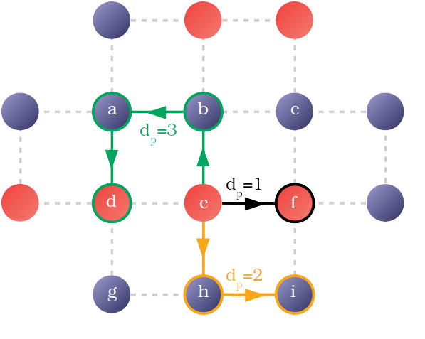
Figure 2: Scheme of three different prospection paths corresponding to three different prospection lengths $d_{p}=1$ (black), $d_{p}=2$ (yellow) and $d_{p}=3$ (green). The patches that are already visited are marked in red (so they add $0$ to the payoff), while the unvisited ones appear in blue (so they add $1$ to the payoff). The payoff assigned in each one of the paths depicted would be a) $E_{f}=0$ to option $f$ for $d_{p}=1$, b) $E_{i}=(1+1)/2=1$ to option $h$ for $d_{p}=2$, and $E=(1+1+0)/3=2/3$ to option $b$ for $d_{p}=3$.

The walker keeps in memory its previous trajectory during a characteristic number of steps. In particular, the visits are remembered by the virtual subject during a time $\tau$ obtained from the exponential distribution $P(\tau)=\frac{1}{\tau_{m}}e^{-\frac{t}{\tau_{m}}}$, with $\tau_{m}$ then representing the characteristic timescale of memory. After this time, the walker will forget that this particular patch has been previously visited and will contribute as a non-visited patch for computing the corresponding payoffs.

As a result, the algorithm will assign lower payoffs to the options that it remembers having visited and/or that are adjacent to regions that it remembers having visited. So, according to equation $2$ in the Main Text, the probability to choose those options will decrease, so leading the virtual subject to regions that are still unvisited (or at least it does not remember having visited before). A larger prospection length $d_{p}$ allows the walker to sample the state of further regions and to compute the payoff the information of distant patches, but this will be only efficient if the memory parameter $\tau_{m}$ is large enough.

Successive prospections of the paths available in each direction are carried out at random among all possible ones of length $d_{p}$, and so values of the payoffs and the probabilities $p_{i}$ are continuously updated. Note that for a given value of $d_{p}$ the number of paths that can be prospected is of the order of $\sim 4^{d_{p}}$ (if assuming that all bonds between neighbours are available). The algorithm makes the virtual walker to move to one of the available nodes according to the decision criterion described in the Main Text. After each single prospection of one path in each direction, the Shannon’s entropy $S=\sum_{i}-p_{i}\ln p_{i}$ is computed; if the value falls below a fixed threshold $S_{th}$, the walker makes a move according to the probabilities $p_{i}$ computed at that time (we have checked to decide according to the highest probability does not change qualitatively the walker dynamics). On the contrary, if $S>S_{th}$ then the prospection process continues. However, we additionally introduce a rule such that the maximum number of prospections is limited to $100$ to avoid (extremely unusual) situations in which $S$ would never decay below $S_{th}$ because all options available persistently exhibit very similar payoffs. We have carefully checked that this rule doesn’t modify any of the results reported in a significant way.

II.2 Coverage time study

The results of the algorithm shown in the Main Text have been obtained under the same conditions that in the task presented to the human subjects; this is, for $49$-step trajectories through the $7x7$ lattice with the same topological structure as presented in Fig. 3 in the Main Text. However, for the sake of completeness we also analyze here the dynamics of the prospective algorithm when removing the limitation of $49$ moves, and measuring instead the number of moves it takes to cover all the patches. This gives us an additional insight about the navigation efficiency of the algorithm as a function of the memory and prospection parameters, $\tau_{m}$ and $d_{p}$. In particular, we study the mean coverage time ($T_{Cov}$) (this is, the mean time required to cover all sites in the lattice). Minimization of this magnitude would then give an estimation of the navigation efficiency of the algorithm.

The main conclusion we can extract (as one can deduce from the results in Fig. 3) is that the ability to prospect future paths (so, having a large $d_{p}$) is useless unless the individual has good memory skills (this is, a large $\tau_{m}$ value in our context). This makes clear sense, as when the walker cannot remember the previously visited patches (low values of $\tau_{m}$), the optimal strategy consists of removing prospection ($d_{p}=1$); in that case the information provided by further patches represents just useless noise as the walker always sees them as non-visited patches. On the other side, for large $\tau_{m}$ the walker can correctly identify the previously visited patches (large values of $\tau_{m}$), so then progressively higher prospection lengths $d_{p}$ are found to optimize the coverage of the structure and the search of a target.

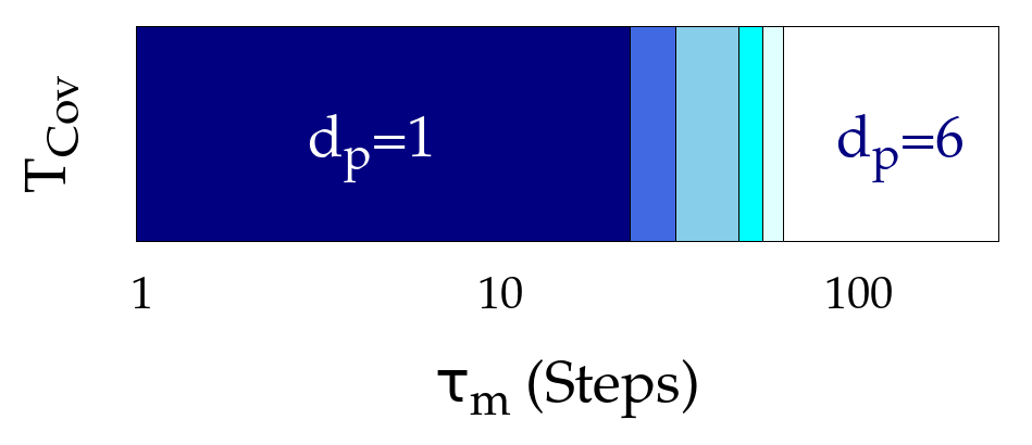
Figure 3: Prospection length $d_{p}$ that minimizes the coverage process, i. e., the parameter that provides a performance that minimizes then mean coverage time ($T_{Cov}$) for different values of the memory time $\tau_{m}$.

II.3 Distributed prospection lengths

Assigning a constant prospection length $d_{p}$ to all the prospected paths may seem rather unrealistic. Human individuals are expected instead to prospect paths with different lengths depending on the specific situation (complexity, number of choices available, etc). The results reported in fig 5 b) in the Main Text also support this statement (the number of gazed patches is not fixed to a constant number but exhibits a variation which spans almost one order of magnitude).

We have studied then our algorithm for the case when a distribution of $d_{p}$ is introduced instead of a constant value. We have tried in particular a distribution $P(d_{p})\propto\frac{1}{d_{p}^{\gamma}}$ (for $d_{p}\geq 1$), with $\sum_{d_{p}=1}^{\infty}P(d_{p})=1$ to guarantee normalization. For $\gamma\to\infty$, the paths are then fixed to $d_{p}=1$, so the prospection algorithm is only to identify whether the neighbour nodes have been visited or not. On the other side, for $\gamma\rightarrow 0$ the probability is uniformly distributed among all $d_{p}$ values (at practice we limit $d_{p}$ to $1\leq d_{p\leq 6}$ since much larger values would be absurd, given the 7x7 maze we have used). Figure 4 reports that sampling a small (but not negligible) number of long paths combined with a majority of short paths (as happens for intermediate $\gamma$ values) is sufficient to recover the same dynamics as obtained for a large fixed $d_{p}$ value. This can be seen by comparing results obtained for lower values of $\gamma$ to those of large values of $d_{p}$, which are extremely similar. This result is remarkable from an evolutionary perspective, since it suggests that improving navigation efficiency would not necessarily require to process much more information continually (note that the number of paths available for prospection grows in general as $n^{d_{p}}$ for a sequential decision task in which $n$ choices are given to the subject at any step, so processing costs grow exponentially with $d_{p}$). Instead, having the ability to carry out longer prospections and use this ability just promptly would be enough to increase efficiency significantly.

Figure 4: Averaged total number of covered patches after the 49 steps trajectory as a function of the memory time $\tau_{m}$ for the Virtual Walker. The graph a) corresponds to a walker prospecting with a fixed for prospection length $d_{p}$ and the graph b), to a walker prospecting with a variable prospection $d_{p}$ obtained from a power-law distribution with exponent $\gamma$.

By exploring the whole range of $\gamma$ and $\tau_{m}$ values, we can divide the parameter phase space into four regions (figure 5 b)), analogously as shown in the Main Text for fixed $d_{p}$. The region I produces an averaged performance that visits less patches than the individuals in any of the experimental graphs. The region II produces a performance which lies between the results obtained between Circular Ordered and Disordered. The region III overcomes the results for the Circular Ordered performance but not for the Rectangular. The region IV, finally, outperforms all the experimental results. The regions are equivalent to the obtained for fixed path lengths. Again, this shows that distributed values of $d_{p}$ can be used to obtain higher navigation efficiencies without consuming much higher times of information processing.

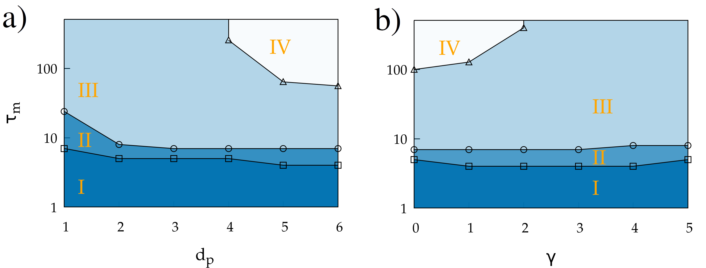
Figure 5: Diagram for the walker covered patches in comparison with experimental results. Regime $I$ corresponds to a worse averaged performance than all geometries. Regime $II$ corresponds to a better performance than in Circular Disordered. Regime $III$ corresponds to a better performance than in Circular Ordered and Disordered. Regime $IV$ corresponds to a better performance than in all geometries. The graph a) corresponds to a walker prospecting with a fixed for prospection length $d_{p}$ and the graph b), to a walker prospecting with a variable prospection $d_{p}$ obtained from a power-law distribution with exponent $\gamma$.

II.4 Robustness of the power-law exponent for the distribution of decision times

We have reported in the Main Text that the decision time for the walker, defined as the number of required prospected paths that makes $S<S_{th}$, exhibits again the same power-law distribution (with exponent $-3$) as the Gaussian working example. The results in Fig. 5 in the Main Text correspond to the values $t_{m}$ and $d_{p}$ obtained from fits to the experimental data. Here we provide an analysis to check that the $-3$ exponent remains as a characteristic feature of the algorithm, independent of the memory and prospection parameters, as well as the threshold $S_{th}$ used in the algorithm.

First, in Fig. 6a we show the explicit dependence on the entropy threshold, and verify that the power-law behavior is kept as long as reasonable values of this parameter are chosen (extreme choices, with, $S_{th}\rightarrow 0$ for example, would modify the results, but we stress that this represents a rather unrealistic case for the purposes here). While the behavior of the walker is equivalent for different $S_{th}$, we fix it in our results in the Main Text to $S_{th}=0.5$ so it can be conveniently applied to all choices in our maze, regardless the algorithm has two, three or four options available at that movement. On the other side, we observe at Fig. 6b that neither variations in $d_{p}$ nor $\tau_{m}$ modify significantly the $\sim n^{-3}$ behavior as long as some significant level of memory and prospection is kept.

We stress that the classical SPRT criterion, as well as other variations we have numerically explored, are unable to reproduce the $-3$ exponent and would lead to much smaller exponents and/or faster (exponential-like) decays in $P(n)$. This, together with the robustness analysis reported here, provides significant robustness to the entropy threshold criterion proposed here.

Figure 6: a) Distribution of the number of prospections $n$ performed by the walker to force the entropy $S$ to fall below the threshold $S_{th}$. The parameters $d_{p}$ and $\tau_{m}$ are fixed to $d_{p}=6$ and $\tau_{m}=100$, respectively, while different $S_{th}$ are explored. b) Distribution of the number of prospections $n$ performed by the walker to force the entropy $S$ to fall below the threshold $S_{th}$. The parameter $S_{th}$ is fixed to $S_{th}=0.5$, while different $d_{p}$ and $\tau_{m}$ are explored.