On Roli’s Cube

Abstract

First described in 2014, Roli’s cube $\mathcal{R}$ is a chiral $4$-polytope, faithfully realized in Euclidean $4$-space (a situation earlier thought to be impossible). Here we describe $\mathcal{R}$ in a new way, determine its minimal regular cover, and reveal connections to the Möbius-Kantor configuration.

Key Words: regular and chiral polytopes; realizations of polytopes

AMS Subject Classification (2000): Primary: 51M20. Secondary: 52B15.

1 Introduction

Actually Roli’s cube $\mathcal{R}$ isn’t a cube, although it does share the $1$-skeleton of a $4$-cube. First described by Javier (Roli) Bracho, Isabel Hubard and Daniel Pellicer in [3], $\mathcal{R}$ is a chiral $4$-polytope of type $\{8,3,3\}$, faithfully realized in $\mathbb{E}^{4}$ (a situation earlier thought impossible). Of course, Roli didn’t himself name $\mathcal{R}$; but the eponym is pleasing to his colleagues and has taken hold.

Chiral polytopes with realizations of ‘full rank’ had (incorrectly) been shown not to exist by Peter McMullen in [11, Theorem 11.2]. Mind you, these objects do seem to be elusive. Pellicer has proved in [15] that chiral polytopes of full rank can exist only in ranks $4$ or $5$.

Roli’s cube $\mathcal{R}$ was constructed in [3] as a colourful polytope, starting from a hemi-$4$-cube in projective $3$-space. (For more on this, see Section 3.) The construction given here in Section 6 is a bit different, though certainly closely related. In Section 7 we can then easily manufacture the minimal regular cover $\mathcal{T}$ for $\mathcal{R}$, and give both a presentation and faithful representation for its automorphism group. Along the way, we encounter both the Möbius-Kantor Configuration $8_{3}$ and the regular complex polygon $3\{3\}3$.

In what follows, we can make our way with concrete examples, so we won’t need much of the general theory of abstract regular or chiral polytopes and their realizations. We refer the reader to [13], [12] and [16] for more.

2 The $4$-cube: convex, abstract and colourful

The most familiar of the regular convex polytopes in Euclidean space $\mathbb{E}^{4}$ is surely the $4$-cube $\mathcal{P}=\{4,3,3\}$. A familiar projection of $\mathcal{P}$ into $\mathbb{E}^{3}$ is displayed in Figure 1.

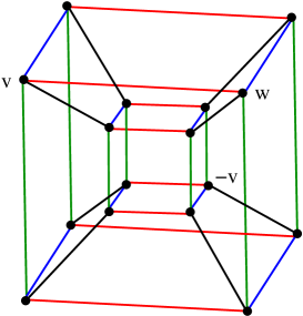
Figure 1: A $2$-dimensional look at a $3$-dimensional projection of the $4$-cube.

Let us equip $\mathbb{E}^{4}$ with its usual basis $b_{1},\ldots,b_{4}$ and inner product. Then we may take the vertices of $\mathcal{P}$ to be the $16$ sign change vectors

$$e=(\varepsilon_{1},\ldots,\varepsilon_{4})\in\{\pm 1\}^{4}.$$ (1)

At any such vertex there is an edge (of length $2$) running in each of the $4$ coordinate directions, so that $\mathcal{P}$ has $32=\frac{16\cdot 4}{2}$ edges. Similarly we count the $24$ squares $\{4\}$ as faces of dimension $2$. Finally, $\mathcal{P}$ has $8$ facets; these faces of dimension $3$ are ordinary cubes $\{4,3\}$. They lie in four pairs of supporting hyperplanes orthogonal to the coordinate axes. It is enjoyable to hunt for these faces in Figure 2, where the $8$ parallel edges in each of the coordinate directions have colours black, red, blue and green, respectively.

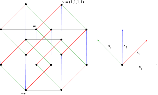
Figure 2: The most symmetric $2$-dimensional projection of the $4$-cube.

Let us turn to the symmetry group $G$ for $\mathcal{P}$. Each symmetry $\gamma$ is determined by its action on the vertices, which clearly can be permuted with sign changes in all possible ways. Thus $G$ has order $2^{4}\cdot 4!=384$, and we may think of it as being comprised of all $4\times 4$ signed permutation matrices.

In fact, $G$ can be generated by reflections $\rho_{0},\rho_{1},\rho_{2},\rho_{3}$ in hyperplanes. Here $\rho_{0}$ negates the first coordinate $x_{1}$ (reflection in the coordinate hyperplane orthogonal to $b_{1}$); and, for $1\leqslant j\leqslant 3$, $\rho_{j}$ transposes coordinates $x_{j},x_{j+1}$ (reflection in the hyperlane orthogonal to $b_{j}-b_{j+1}$).

Note that the reflection in the $j$-th coordinate hyperplane is $\rho_{0}^{\rho_{1}\cdots\rho_{j-1}}$ for $1\leqslant j\leqslant 4$. (We use the notation $\gamma^{\eta}:=\eta^{-1}\gamma\eta$.) The product of these $4$ special reflections, in any order, is the central element $\zeta:t\mapsto-t$. It is easy to check as well that

$$\zeta=(\rho_{0}\rho_{1}\rho_{2}\rho_{3})^{4}\;.$$ (2)

The Petrie symmetry $\pi=\rho_{0}\rho_{1}\rho_{2}\rho_{3}$ therefore has period $8$.

For purposes of calculation, we note that $G\simeq C_{2}^{4}\rtimes S_{4}$ is a semidirect product. Under this isomorphism, each $\gamma\in G$ factors uniquely as $\gamma=e\mu$, where $\mu\in S_{n}$ is a permutation of $\{1,\ldots,4\}$ (labelling the coordinates); and $e$ is a sign change vector, as in (1). Note that

$$e^{\mu}=(\varepsilon_{1},\varepsilon_{2},\varepsilon_{3},\varepsilon_{4})^{\mu}=(\varepsilon_{(1)\mu^{-1}},\varepsilon_{(2)\mu^{-1}},\varepsilon_{(3)\mu^{-1}},\varepsilon_{(4)\mu^{-1}})\,.$$

Now really $\gamma$ is a signed permutation matrix. But it is convenient to abuse notation, keeping in mind that each $e$ corresponds to a diagonal matrix of signs and each $\mu$ to a permutation matrix. Thus we might write

$$\pi=\rho_{0}\rho_{1}\rho_{2}\rho_{3}=(-1,1,1,1)\cdot(4,3,2,1)=\left[\begin{array}[]{rrrr}0&0&0&-1\\ 1&0&0&0\\ 0&1&0&0\\ 0&0&1&0\end{array}\right]\;.$$ (3)

Next we use the group $G=\langle\rho_{0},\rho_{1},\rho_{2},\rho_{3}\rangle$ to remanufacture the cube. In this (geometric) version of Wythoff’s construction [7, §2.4] we choose a base vertex $v$ fixed by the subgroup $G_{0}:=\langle\rho_{1},\rho_{2},\rho_{3}\rangle$ (which permutes the coordinates in all ways). Thus, $v=c(1,1,1,1)$ for some $c\in\mathbb{R}$. To avoid a trivial construction we take $c\neq 0$, so, up to similarity, we may use $c=1$. Then the orbit of $v$ under $G$ is just the set of $16$ points in (1); and their convex hull returns $\mathcal{P}$ to us. Since $G_{0}$ is the full stabilizer of $v$ in $G$, the vertices correspond to right cosets $G_{0}\gamma$.

The beauty of Wythoff’s construction is that all faces of $\mathcal{P}$ can be constructed in a similar way by induction on dimension ([13, Section 1B], [4] and [12]). For example, the vertices $v=(1,1,1,1)$ and $v\rho_{0}=(-1,1,1,1)$ of the base edge of $\mathcal{P}$ are just the orbit of $v$ under the subgroup $G_{1}:=\langle\rho_{0},\rho_{2},\rho_{3}\rangle$; and edges of $\mathcal{P}$ correspond to right cosets of the new subgroup $G_{1}$. Furthermore, a more careful look reveals that a vertex is incident with an edge just when the corresponding cosets have non-trivial intersection.

Pursuing this, we see that the face lattice of $\mathcal{P}$ can be recontructed as a coset geometry based on subgroups

$$G_{0},G_{1},G_{2},G_{3},\;\;\mathrm{where}\;G_{j}:=\langle\rho_{0},\ldots,\widehat{\rho_{j}},\ldots,\rho_{3}\rangle.$$ (4)

From this point of view, $\mathcal{P}$ becomes an abstract regular $4$-polytope, a partially ordered set whose automorphism group is $G$. Notice that the distinguished subgroups in (4) provide the proper faces in a flag in $\mathcal{P}$, namely a mutually incident vertex, edge, square and $3$-cube.

The crucial structural property of $G$ is that it should be a string C-group with respect to the generators $\rho_{j}$. A string C-group is a quotient of a Coxeter group with linear diagram under which an ‘intersection condition’ on subgroups generated by subsets of generators, such as those in (4), is preserved [13, Sections 2E].

For the $4$-cube $\mathcal{P}$, $G$ is actually isomorphic to the Coxeter group $B_{4}$ with diagram

$${\bullet}\frac{4}{\;\;\;\;\;\;\;}{\bullet}\frac{3}{\;\;\;\;\;\;\;}{\bullet}\frac{3}{\;\;\;\;\;\;\;}{\bullet}$$ (5)

Comparing the geometric and abstract points of view, we say that the convex $4$-cube is a realization of its face lattice (the abstract $4$-cube).

When we think of a polytope from the abstract point of view, we often use the term rank instead of ‘dimension’. An abstract polytope $\mathcal{Q}$ is said to be regular if its automorphism group is transitive on flags (maximal chains in $\mathcal{Q}$). Intuitively, regular polytopes have maximal symmetry (by reflections). Next up are chiral polytopes, with exactly two flag orbits and such that adjacent flags are always in different orbits (so maximal symmetry by rotations, but without reflections).

We will soon encounter less familiar abstract regular or chiral polytopes, with their realizations. For a first example, suppose that we map (by central projection) the faces of $\mathcal{P}$ onto the $3$-sphere $\mathbb{S}^{3}$ centred at the origin. We can then reinterpret $\mathcal{P}$ as a regular spherical polytope (or tessellation), with the same symmetry group $G$. Now the centre of $G$ is the subgroup $\langle\zeta\rangle$ of order $2$. The quotient group $G/\langle\zeta\rangle$ has order $192$ and is still a string C-group. The corresponding regular polytope is the hemi-$4$-cube $\mathcal{H}=\{4,3,3\}_{4}$, now realized in projective space $\mathbb{P}^{3}$ [13, Section 6C]; see Figure 3. By (2), the product of the four generators of $G/\langle\zeta\rangle$ has order $4$; this is recorded as the subscript in the Schläfli symbol for $\mathcal{H}$.

Now we can outline the construction of Roli’s cube given in [3].

3 Colourful polyopes

The image in Figure 1 or on the left in Figure 2 can just as well be understood as a graph $\mathcal{G}$, namely the $1$-skeleton of the $4$-cube $\mathcal{P}$. In fact, we can recreate the abstract (or combinatorial) structure of $\mathcal{P}$ from just the edge colouring of $\mathcal{G}$: for $0\leqslant j\leqslant 4$, the $j$-faces of $\mathcal{P}$ can be identified with the components of those subgraphs obtained by keeping just edges with some selection of the $j$ colours (over all such choices). We therefore say that $\mathcal{P}$ is a colourful polytope.

Such polytopes were introduced in [1]. In general, one begins with a finite, connected $d$-valent graph $\mathcal{G}$ admitting a (proper) edge colouring, say by the symbols $1,\ldots,d$. Thus each of the colours provides a $1$-factor for $\mathcal{G}$. The graph $\mathcal{G}$ determines an (abstract) colourful polytope $\mathcal{P}_{\mathcal{G}}$ as follows. For $0\leqslant j\leqslant d$, a typical $j$-face $(C,v)$ is identified with the set all vertices of $\mathcal{G}$ connected to a given vertex $v$ by a path using only colours from some subset $C$ of size $j$ taken from $\{1,\ldots,d\}$. The $j$-face $(C,v)$ is incident with the $k$-face $(D,w)$ just when $C\subseteq D$ and $w$ can be reached from $v$ by a $D$-coloured path. (This means that $j\leqslant k$; and we can just as well take $w=v$. The minimal face of rank $-1$ in $\mathcal{P}_{\mathcal{G}}$ is formal.) Notice that $\mathcal{P}_{\mathcal{G}}$ is a simple $d$-polytope whose $1$-skeleton is just $\mathcal{G}$ itself. From [1, Theorem 4.1], the automorphism group of $\mathcal{P}_{\mathcal{G}}$ is isomorphic to the group of colour-preserving graph automorphisms of $\mathcal{G}$. (Such automorphisms are allowed to permute the $1$-factors.)

It is easy to see that the hemi-$4$-cube $\mathcal{H}$ is also colourful. Its $1$-skeleton is the complete bipartite graph $K_{4,4}$ found in Figure 3. We obtain this graph from Figure 1 or Figure 2 by identifying antipodal pairs of points, like $v$ and $-v$.

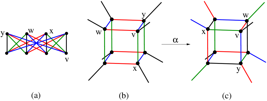
Figure 3: The graph $K_{4,4}$ in (a) is the $1$-skeleton of the hemi-$4$-cube $\{4,3,3\}_{4}$ (b),(c).

If we lift $\mathcal{H}$, as it is now, to $\mathbb{S}^{3}$, we regain the coloured $4$-cube $\mathcal{P}$. Now keep $K_{4,4}$ embedded in $\mathbb{P}^{3}$, as in Figure 3. But, following [3], observe that $K_{4,4}$ admits the automorphism $\alpha$ which cyclically permutes, say, the first three vertices $y,w,x$ in the top block, leaving the rest fixed. Clearly, $\alpha$ is a non-colour-preserving automorphism of $K_{4,4}$, so its effect is to recolour $12$ of the edges in the embedded graph. On the abstract level nothing has changed for the resulting colourful polytope; it is still the hemi-$4$-cube $\mathcal{H}$. But faces of ranks $2$ and $3$ are now differently embedded in $\mathbb{P}^{3}$. For example, the red-blue $2$-face on $v$, which is planar in Figure 3(b), becomes a helical quadrangle Figure 3(c) and thereby acquires an orientation. According to Definition 4.1, these helical polygons are Petrie polygons for the standard realization of $\mathcal{H}$ in Figure 3(b).

The newly coloured geometric object, which we might label $\mathcal{H}^{R}$, is a chiral realization of the abstract regular polytope $\mathcal{H}$. Comforted by the fact that $\mathbb{P}^{3}$ is orientable, we could just as well apply $\alpha^{-1}$ to obtain the left-handed version $\mathcal{H}^{L}$. These two enantiomorphs are oppositely embedded in $\mathbb{P}^{3}$, though both remain isomorphic to $\mathcal{H}$ as partially ordered sets. If we lift either enantiomorph to $\mathbb{S}^{3}$, we obtain a chiral $4$-polytope faithfully realized in $\mathbb{E}^{4}$ [3, Theorem 2]. This is Roli’s cube $\mathcal{R}$.

Next we set the stage for a slightly different construction of $\mathcal{R}$, without the use of $\mathbb{P}^{3}$.

4 Petrie polygons of the $4$-cube

Let us consider the progress of the base vertex $v=(1,1,1,1)$ as we apply successive powers of $\pi$ in (3). We get a centrally symmetric $8$-cycle of vertices

$$v\rightarrow(1,1,1,-1)\rightarrow(1,1,-1,-1)\rightarrow(1,-1,-1,-1)\rightarrow-v=(-1,-1,-1,-1)\rightarrow\ldots\;.$$

Starting from $v$ in Figure 2 we therefore proceed in coordinate directions 4, 3, 2, 1 (indicated by different colours), then repeat again. This traces out the peripheral octagon $\mathcal{C}$, which in fact is a Petrie polygon for $\mathcal{P}$.

Definition 4.1.

A Petrie polygon of a $3$-polytope is an edge-path such that any $2$ consecutive edges, but no $3$, belong to a $2$-face. We then say that a Petrie polygon of a $4$-polytope $\mathcal{Q}$ is an edge-path such that any $3$ consecutive edges, but no $4$, belong to (a Petrie polygon of) a facet of $\mathcal{Q}$.

For the cube $\mathcal{P}$, the parenthetical condition is actually superfluous; compare [9].

Clearly, we can begin a Petrie polygon at any vertex, taking any of the $4!$ orderings of the colours. But this counts each octagon in $16$ ways. We conclude that $\mathcal{P}$ has $24$ Petrie polygons. What we really use here is the fact that $G$ is transitive on vertices, and that at any fixed vertex, $G$ permutes the edges in all possible ways. We see that $G$ acts transitively on Petrie polygons.

But the (global) stabilizer of $\mathcal{C}$ (constructed above with the help of $\pi$ and $v$) is the dihedral group $K$ of order $16$ generated by $\mu_{0}=\rho_{0}\rho_{2}\rho_{3}\rho_{2}=(-1,1,1,1)\cdot(2,4),$ and $\mu_{1}=\mu_{0}\pi=\rho_{2}\rho_{3}\rho_{2}\rho_{1}\rho_{2}\rho_{3}=(1,1,1,1)\cdot(1,4)(2,3)$. (Such calculations are routine using either signed permutation matrices or the decomposition in $C_{2}^{4}\rtimes S_{4}$. Note that any $4$ consecutive vertices of $\mathcal{C}$ form a basis of $\mathbb{E}^{4}$.) We confirm that $\mathcal{P}$ has $24=384/16$ Petrie polygons.

Now we move to the rotation subgroup

$$G^{+}=\langle\rho_{0}\rho_{1},\rho_{1}\rho_{2},\rho_{2}\rho_{3}\rangle.$$

It has order $192$ and consists of the signed permutation matrices of determinant $+1$. Note that $K<G^{+}$. Thus, under the action of $G^{+}$, there are two orbits of Petrie polygons of $12$ each. Let’s label these two chiral classes $R$ and $L$ for right- and left-handed, taking $\mathcal{C}$ in class $R$.

The two chiral classes must be swapped by any non-rotation, such as any $\rho_{j}$. To distinguish them, we could take the determinant of the matrix whose rows are any $4$ consecutive vertices on a Petrie polygon. The two chiral classes $R$ and $L$ then have determinants $+8$, respectively, $-8$. Or starting from a common vertex, the edge-colour sequence along a polygon in one class is an odd permutation of the colour sequence for a polygon in the other class.

The inner octagram ${\mathcal{C}}^{*}$ in Figure 2 is another Petrie polygon. Start at the vertex $w=(v)\rho_{1}\rho_{0}\rho_{1}=(1,-1,1,1)$ which is adjacent to $v$ along a red edge; then proceed in directions 4, 1, 2, 3 and repeat. However, the remaining Petrie polygons appear in less symmetrical fashion in Figure 2.

Note that $\mu_{0}$ actually acts on the diagram in Figure 2 as a reflection in a vertical line, whereas $\pi$ rotates the octagon $\mathcal{C}$ and octagram $\mathcal{C}^{*}$ in opposite senses. On the other hand, $\mu_{2}=\rho_{1}\rho_{2}\rho_{0}\rho_{1}=(1,-1,1,1)\cdot(1,3)$ is an element of $G^{+}$ which swaps $\mathcal{C}$ and $\mathcal{C}^{*}$. Thus there are $6$ such unordered pairs like $\mathcal{C},\mathcal{C}^{*}$ in class $R$ and another $6$ pairs in class $L$.

Remark 4.2.

It can be shown that Figure 2 is the most symmetric orthogonal projection of $\mathcal{P}$ to a plane [6, §13.3]. Since all edges after projection have a common length, we may say that this projection is isometric.

The Petrie symmetry $\pi$ is one instance of a Coxeter element in the group $G=B_{4}$, namely a product of the four generators in some order. All such Coxeter elements are conjugate. Each of them has invariant planes which give rise to the sort of orthogonal projection displayed in Figure 2. A procedure for finding these planes is detailed in [10, 3.17]. For $\pi$, the two planes are spanned by the rows of

$$\left[\begin{array}[]{rrrr}\frac{1}{\sqrt{2}}&\frac{1}{2}&0&\frac{-1}{2}\\ 0&\frac{1}{2}&\frac{1}{\sqrt{2}}&\frac{1}{2}\end{array}\right]\;\mathrm{and}\;\left[\begin{array}[]{rrrr}\frac{1}{\sqrt{2}}&\frac{-1}{2}&0&\frac{1}{2}\\ 0&\frac{1}{2}&\frac{-1}{\sqrt{2}}&\frac{1}{2}\end{array}\right].$$

These planes are orthogonal complements; and $\pi$ acts on them by rotations through $45^{\circ}$ and $135^{\circ}$, respectively. Figure 2 results from projecting $\mathcal{P}$ onto the first plane. $\square$

5 The map $\mathcal{M}$ and the Möbius-Kantor Configuration $8_{3}$

Look again at the companion Petrie polygons $\mathcal{C},\mathcal{C}^{*}$ in Figure 2. Now working around the rim clockwise from $v$ delete the edges coloured blue, red, black, green, and repeat. We are left with the trivalent graph $\mathcal{L}$ displayed in Figure 4.

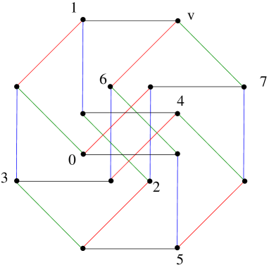
Figure 4: The Levi graph $\mathcal{L}=\{8\}+\{\frac{8}{3}\}$ for the configuration $8_{3}$.

In fact, $\mathcal{L}$ is the generalized Petersen graph $\{8\}+\{\frac{8}{3}\}$, studied in detail by Coxeter in [5, Section 5]. The graph is $2$-arc transitive, so that its automorphism group has order $96=16\cdot 3\cdot 2^{2-1}$ [2, Chapter 18]. We return to this group later.

We have labelled alternate vertices of $\mathcal{L}$ by the residues $0,1,2,3,4,5,6,7\pmod{8}$. These will represent the points in a Möbius-Kantor configuration $8_{3}$. The remaining (unlabelled) vertices of $\mathcal{L}$ represent the $8$ lines in the configuration. Thus we have lines $013$ (represented by the ‘north-west’ vertex $(-1,-1,1,1)$), $124$, $235$, and so on, including line $671$ represented by $v$.

Notice that we can interpret the configuration as being comprised of two quadrangles with vertices $0,2,4,6$ and $1,3,5,7$, each inscribed in the other: vertex $0$ lies on edge $13$, vertex $1$ lies on edge $24$, and so on.

So far this configuration $8_{3}$ is purely abstract. In fact, it can be realized as a point-line configuration in a projective (or affine) plane over any field in which

$$z^{2}-z+1=0$$

has a root, certainly over $\mathbb{C}$. However, $8_{3}$ cannot be realized in the real plane.

Coxeter made other observations in [5], including the fact that the graph $\mathcal{L}$ is a sub-$1$-skeleton of the $4$-cube. Altogether $\mathcal{L}$ contains $6$ Petrie polygons, which we can briefly describe by their alternate vertices:

$$\begin{array}[]{ccc}0246(=\mathcal{C}^{*})&0541&1256\\ 1357(=\mathcal{C})&2367&0743\\ \end{array}$$

Hence, the configuration can be regarded as a pair of mutually inscribed quadrangles in three ways.

Observe that each edge of $\mathcal{L}$ lies on exactly two of the $6$ octagons. For example, the top edge with vertices labelled $1$ and $v$ lies on octagons $1357$ and $1256$. (It does not matter that two such octagons then share a second edge opposite the first.) Furthermore, each vertex lies on the three octagons determined by choices of two edges. We can thereby construct a $3$-polytope $\mathcal{M}$ of type $\{8,3\}$, with $6$ octagonal faces, whose $1$-skeleton is $\mathcal{L}$. In short, $\mathcal{M}$ is realized by substructures of the $4$-cube $\mathcal{P}$.

Moving sideways, we can reinterpret $\mathcal{M}$ in a more familiar topological way as a map on a compact orientable surface of genus $2$. Recall that $\mathcal{M}$ is covered by the tessellation $\{8,3\}$ of the hyperbolic plane, as indicated in Figure 5.

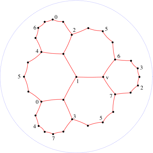
Figure 5: Part of the tessellation $\{8,3\}$ of the hyperbolic plane.

Now return to $\mathbb{E}^{4}$ where the combinatorial structure of $\mathcal{M}$ is handed to us as faithfully realized. Drawing on [8, Section 8.1], we have that the rotation group $\varGamma(\mathcal{M})^{+}$ for $\mathcal{M}$ is generated by two special Euclidean symmetries:

$\sigma_{1}=\pi=\rho_{0}\rho_{1}\rho_{2}\rho_{3}=(-1,1,1,1)\cdot(4,3,2,1)$ (preserving the base octagon $\mathcal{C}$); and

$\sigma_{2}=\rho_{3}\rho_{2}\rho_{1}\rho_{3}=(1,1,1,1)\cdot(1,2,4)$ (preserving the base vertex $v$ on $\mathcal{C}$).

The order of $\varGamma(\mathcal{M})^{+}$ must then be twice the number of edges in $\mathcal{M}$, namely $48$. Let us assemble these and further observations in

Proposition 5.1.

(a) The $3$-polytope $\mathcal{M}$ is abstractly regular of type $\{8,3\}$, here realized in $\mathbb{E}^{4}$ in a geometrically chiral way.

(b) The rotation subgroup $\varGamma(\mathcal{M})^{+}=\langle\sigma_{1},\sigma_{2}\rangle$ has order $48$ and presentation

$$\langle\sigma_{1},\sigma_{2}\,|\,\sigma_{1}^{8}=\sigma_{2}^{3}=(\sigma_{1}\sigma_{2})^{2}=(\sigma_{1}^{-3}\sigma_{2})^{2}=1\rangle$$ (6)

(c) The full automorphism group $\varGamma(\mathcal{M})$ has order $96$ and presentation

$$\langle\tau_{0},\tau_{1},\tau_{2}\,|\,\tau_{0}^{2}=\tau_{1}^{2}=\tau_{2}^{2}=(\tau_{0}\tau_{1})^{8}=(\tau_{1}\tau_{2})^{3}=(\tau_{0}\tau_{2})^{2}=((\tau_{1}\tau_{0})^{3}\tau_{1}\tau_{2})^{2}=1\rangle$$ (7)

Proof. We begin with (b), where it is easy to check that the relations in (6) do hold for the matrix group $\langle\sigma_{1},\sigma_{2}\rangle$. By a straightforward coset enumeration [8, Chapter 2], we conclude from the presentation in (6) that the subgroup $\langle\sigma_{1}\rangle$ has the $6$ coset representatives

$$1,\sigma_{1},\sigma_{1}^{2},\sigma_{2}\sigma_{1}^{-1},\sigma_{2}^{2}\sigma_{1},\sigma_{2}\sigma_{1}^{-1}\sigma_{2}.$$

(We abuse notation by passing freely between the matrix group and abstract group.) This finishes (b).

We next note that $\langle\sigma_{1}\rangle\cap\langle\sigma_{2}\rangle=\{1\}$, since $\sigma_{1}^{j}$ fixes $v$ only for $j\equiv 0\pmod{8}$. Now we are justified in invoking [16, Theorem 1(c)], whereby the $3$-polytope $\mathcal{M}$ is regular (rather than just chiral) if and only if the mapping $\sigma_{1}\mapsto\sigma_{1}^{-1},\;\sigma_{2}\mapsto\sigma_{1}^{2}\sigma_{2}$ induces an involutory automorphism $\tau$ of $\varGamma(\mathcal{M})^{+}$. But the new relations induced by applying the mapping to (6) are easily verified formally, or even by matrices. For instance, since $\sigma_{1}\sigma_{2}=\sigma_{2}^{-1}\sigma_{1}^{-1}$, we have

$$(\sigma_{1}^{2}\sigma_{2})^{3}=(\sigma_{1}\sigma_{2}^{-1}\sigma_{1}^{-1})^{3}=\sigma_{1}\sigma_{2}^{-3}\sigma_{1}^{-1}=1.$$

Thus $\mathcal{M}$ is abstractly regular and $\varGamma(\mathcal{M})$ has order $96$. The presentation in (7) follows at once by extending $\varGamma(\mathcal{M})^{+}$ by $\langle\tau\rangle$, then letting $\tau_{0}:=\tau,\tau_{1}:=\tau\sigma_{1},\tau_{0}:=\tau\sigma_{1}\sigma_{2}$.

It remains to check that our realization is geometrically chiral. This means that $\tau$ is not represented by a symmetry of $\mathcal{M}$ as realized in $\mathbb{E}^{4}$. From the combinatorial structure, $\tau$ would have to swap vertices $1$ and $v$ while preserving the two Petrie polygons on that edge. This means that $\tau$ would have to act just like $\mu_{0}$, that is, just like reflection in a vertical line in Figure 2. But $\mu_{0}$ does not preserve the set of $8$ edges deleted to give $\mathcal{L}$ in Figure 4. $\square$

Remark 5.2.

It is helpful to note that the centre of $\varGamma(\mathcal{M})^{+}$ is generated by $\sigma_{1}^{4}$. Referring to [8, Section 6.6], we find that $\varGamma(\mathcal{M})^{+}$ is isomorphic to the group $\langle-3,4|2\rangle$, which in turn is an extension by $C_{2}$ of the binary tetrahedral group $\langle 3,3,2\rangle$. Indeed, $a=\sigma_{1}^{-1}\sigma_{2}\sigma_{1}^{-1},b=\sigma_{2}\sigma_{1}^{4}$ satisfy $a^{3}=b^{3}=(ab)^{2}\;(=\zeta)$. Thus, $\langle 3,3,2\rangle\triangleleft\varGamma(\mathcal{M})^{+}$.

6 Roli’s cube – a chiral polytope $\mathcal{R}$ of type $\{8,3,3\}$

Under the action of $G^{+}$ we expect to find $4=192/48$ copies of $\mathcal{M}$. To understand this better, recall that there are $12$ Petrie polygons in one chiral class, say $R$. As with $\mathcal{C}$ and $\mathcal{C}^{*}$, each polygon $\mathcal{D}$ is paired with a unique polygon $\mathcal{D}^{*}$ (with the disjoint set of $8$ vertices). For each $\mathcal{D}$ there are then two ways to remove $8$ edges so as to get a copy of $\mathcal{L}$ and hence a copy of $\mathcal{M}$. Since $\mathcal{M}$ has six $2$-faces like $\mathcal{C}$, we once more find $12\cdot 2/6=4$ copies of $\mathcal{M}$.

Each Petrie polygon lies on $2$ copies of $\mathcal{M}$, again from the two ways to remove $8$ edges. For example, $\mathcal{C}$ lies on both $\mathcal{M}$ and $(\mathcal{M})\mu_{0}$. (The same is true for $\mathcal{C}^{*}$.)

The pointwise stabilizer in $G^{+}$ of the base edge joining $v=(1,1,1,1)$ and $(v)\mu_{0}=(-1,1,1,1)$ must consist of pure, unsigned even permutations of $\{2,3,4\}$. Therefore it is generated by

$$\sigma_{3}:=\rho_{2}\rho_{3}=(1,1,1,1)\cdot(2,4,3).$$

It is easy to check that $G^{+}=\langle\sigma_{1},\sigma_{2},\sigma_{3}\rangle$.

Since three consecutive edges of a Petrie polygon lie on two adjacent square faces in a cubical facet of of $\mathcal{P}$, it must be that every vertex of $\mathcal{R}$ has the same vertex-figure as $\mathcal{P}$, thus of tetrahedral type $\{3,3\}$.

We have enumerated and (implicitly) assembled the faces of a $4$-polytope $\mathcal{R}$, faithfully realized in $\mathbb{E}^{4}$ and symmetric under the action of $G^{+}$. Let’s take stock of its proper faces:

rank	stabilizer in $G^{+}$	order	number of faces	type
$0$	$\langle\sigma_{2},\sigma_{3}\rangle$	12	$16$	vertex of cube $\mathcal{P}$
$1$	$\langle\sigma_{1}\sigma_{2},\sigma_{3}\rangle$	6	$32$	edge of $\mathcal{P}$
$2$	$\langle\sigma_{1},\sigma_{2}\sigma_{3}\rangle$	16	$12$	Petrie polygons of $\mathcal{P}$ in one class $R$
$3$	$\langle\sigma_{1},\sigma_{2}\rangle$	48	$4$	copy of $\mathcal{M}$

It is not hard to see that our $4$-polytope $\mathcal{R}$ is isomorphic to Roli’s cube, as constructed in [3] and as described in Section 3.

Theorem 6.1.

(a) The $4$-polytope $\mathcal{R}$ is abstractly chiral of type $\{8,3,3\}$. Its symmetry group $\varGamma(\mathcal{R})\simeq G^{+}$ has order $192$ and the presentation

$$\langle\sigma_{1},\sigma_{2},\sigma_{3} | \sigma_{1}^{8}=\sigma_{2}^{3}=\sigma_{3}^{3}=(\sigma_{1}\sigma_{2})^{2}=(\sigma_{2}\sigma_{3})^{2}=(\sigma_{1}\sigma_{2}\sigma_{3})^{2}=1$$ (10)

$$\hskip 56.9055pt(\sigma_{1}^{-3}\sigma_{2})^{2}=1$$

$$\hskip 56.9055pt(\sigma_{1}^{-1}\sigma_{3})^{4}=1\;\;\rangle$$

(b) $\mathcal{R}$ is faithfully realized as a geometrically chiral polytope in $\mathbb{E}^{4}$.

Proof. The relations in (10) are standard for chiral $4$-polytopes [16, Theorem 1]; and we have seen that the relation in (10) is a special feature of the facet $\mathcal{M}$. Enumerating cosets of the subgroup $\langle\sigma_{1},\sigma_{2}\rangle$, which still has order $48$, we find at most the $8$ cosets represented by

$$1,\sigma_{3},\sigma_{3}^{2},\sigma_{3}^{2}\sigma_{1},\sigma_{3}^{2}\sigma_{1}^{2},\sigma_{3}^{2}\sigma_{1}^{2}\sigma_{2},\sigma_{3}^{2}\sigma_{1}^{2}\sigma_{2}^{2},\sigma_{3}^{2}\sigma_{1}^{2}\sigma_{3}.$$

Thus the group defined by (10) and (10) has order at most $384$. But $G^{+}$, where these relations do hold, has order $192$. We require an independent relation. In Section 7, we will see why (10) is just what we need.

To show that $\mathcal{R}$ is abstractly chiral we must demonstrate that the mapping $\sigma_{1}\mapsto\sigma_{1}^{-1},\sigma_{2}\mapsto\sigma_{1}^{2}\sigma_{2},\sigma_{3}\mapsto\sigma_{3}$ does not extend to an automorphism of $G^{+}$. This is easy, since

$$(\sigma_{1}\sigma_{3})^{4}=\zeta\;\mathrm{whereas}\;(\sigma_{1}^{-1}\sigma_{3})^{4}=1.$$ (11)

Clearly, $\mathcal{R}$ is realized in a geometrically chiral way in $\mathbb{E}^{4}$; we have already seen this for its facet $\mathcal{M}$.

Our concrete geometrical arguments should suffice to convince the reader that we really have described here a chiral $4$-polytope identical to the original Roli’s cube. A skeptic can nail home the proof by applying [16, Theorem 1] to the group $G^{+}$, as generated above. $\square$

7 Realizing the Minimal Regular Cover of $\mathcal{R}$

The rotation group $G^{+}$ for the cube has order $192$ and ‘standard’ generators $\rho_{0}\rho_{1},\rho_{1}\rho_{2},\rho_{2}\rho_{3}$. But for our purposes we use either of two alternate sets of generators. We already have

$$\sigma_{1}=(\rho_{0}\rho_{1})(\rho_{2}\rho_{3}),\;\sigma_{2}=(\rho_{3}\rho_{2})(\rho_{1}\rho_{2})(\rho_{2}\rho_{3}),\;\sigma_{3}=\rho_{2}\rho_{3}.$$ (12)

Now we also want

$$\overline{\sigma}_{1}=\sigma_{1}^{-1},\;\overline{\sigma}_{2}=\sigma_{1}^{2}\sigma_{2},\;\overline{\sigma}_{3}=\sigma_{3}.$$ (13)

Recalling our the shorthand for such matrices, we have

$$\sigma_{1}=(-1,1,1,1)\cdot(4,3,2,1);\;\sigma_{2}=(1,1,1,1)\cdot(1,2,4);\;\sigma_{3}=(1,1,1,1)\cdot(2,4,3),$$

and

$$\overline{\sigma}_{1}=(1,1,1,-1)\cdot(1,2,3,4);\;\overline{\sigma}_{2}=(-1,-1,1,1)(1,3,2);\;\overline{\sigma}_{3}=(1,1,1,1)\cdot(2,4,3).$$

We have seen that the group $G^{+}=\langle\sigma_{1},\sigma_{2},\sigma_{3}\rangle$ (with these specified generators) is the rotation (and full automorphism) group of the chiral polytope $\mathcal{R}$ of type $\{8,3,3\}$. From [17, Section 3] we have that the (differently generated) group $\overline{G^{+}}=\langle\overline{\sigma}_{1},\overline{\sigma}_{2},\overline{\sigma}_{3}\rangle$ is the automorphism group for the enantiomorphic chiral polytope $\overline{\mathcal{R}}$ . By generating the common group in these two ways we effectively exhibit right- and left-handed versions of the same polytope.

Our geometrical realization of $\mathcal{R}$ began with the base vertex $v=(1,1,1,1)$ (which also served as base vertex for the $4$-cube $\mathcal{P}$). It is crucial here that $v$ does span the subspace fixed by $\sigma_{1}$ and $\sigma_{2}$. By instead taking $\overline{G^{+}}$ with base vertex $\overline{v}=(-1,1,1,1)$ fixed by $\overline{\sigma}_{2},$ and $\overline{\sigma}_{3}\rangle$, we have a faithful geometric realization of $\overline{R}$, still in $\mathbb{E}^{4}$, of course.

We will soon have good reason to mix $G^{+}$ and $\overline{G^{+}}$ in a geometric way. Each group acts irreducibly on $\mathbb{E}^{4}$. Construct the block matrices, $\kappa_{j}=(\sigma_{j},\overline{\sigma}_{j})$, $j=1,2,3$, now acting on $\mathbb{E}^{8}$ and preserving two orthogonal subspaces of dimension $4$. Obviously we may extend our notation for signed permutation matrices to the cubical group $B_{8}$ acting on $\mathbb{E}^{8}$. Thus, taking the second copy of $\mathbb{E}^{4}$ to have basis $b_{5},b_{6},b_{7},b_{8}$, we may combine our descriptions of $\sigma_{j},\overline{\sigma}_{j}$ to get

$$\kappa_{1} = (-1,1,1,1,1,1,1,-1)\cdot(4,3,2,1)(5,6,7,8),$$

$$\kappa_{2} = (1,1,1,1,-1,-1,1,1)\cdot(1,2,4)(5,7,6),$$

$$\kappa_{3} = \;\;\;\;\;(1,1,1,1,1,1,1,1)\cdot(2,4,3)(6,8,7).$$

Now let $T^{+}=\langle\kappa_{1},\kappa_{2},\kappa_{3}\rangle$. In slot-wise fashion, $\kappa_{1},\kappa_{2},\kappa_{3}$ satisfy relations like those in (10) and (10). From the proof of Theorem 6.1, we conclude that $T^{+}$ has order $384$. We even get a presentation for it.

Recall that the centre of $G^{+}$ is generated by $\zeta=\sigma_{1}^{4}=\overline{\sigma}_{1}^{4}$. Thus the centre of $T^{+}$ has order $4$, with non-trivial elements

$$(\zeta,1)=(\kappa_{1}\kappa_{3})^{4},\;(1,\zeta)=(\kappa_{1}^{-1}\kappa_{3})^{4},\mathrm{and}\;(\zeta,\zeta)=\kappa_{1}^{4}.$$ (14)

(This is at the heart of the proof that $\mathcal{R}$ is abstractly chiral.) Looking at (11), we see that

$$T^{+}/\langle(1,\zeta)\rangle\simeq\varGamma(\mathcal{R}),$$

and thus see the reason for the special relation in (10). Similarly, $T^{+}/\langle(\zeta,1)\rangle\simeq\varGamma(\overline{\mathcal{R}})$. Finally, we have

$$T^{+}/\langle(\zeta,\zeta)\rangle\simeq\varGamma(\mathcal{P})^{+},$$ (15)

the rotation group of the $4$-cube (isomorphic to $G^{+}$ generated in the customary way).

Now $T^{+}$ is clearly isomorphic to the mix $G^{+}\diamondsuit\,\overline{G^{+}}$ described in [14, Theorem 7.2]. Guided by that result, we seek an isometry $\tau_{0}$ of $\mathbb{E}^{8}$ which swaps the two orthogonal subspaces, while conjugating each $\sigma_{j}$ to $\overline{\sigma}_{j}$. It is easy to check that

$$\tau_{0}=(1,1,1,1,1,1,1,1)\cdot(1,5)(2,6)(3,7)(4,8)$$

does the job. We find that $T^{+}$ is the rotation subgroup of a string C-group $T=\langle\tau_{0},\tau_{1},\tau_{2},\tau_{3}\rangle$, where $\tau_{1}=\tau_{0}\kappa_{1},\tau_{2}=\tau_{0}\kappa_{1}\kappa_{2},\tau_{3}=\tau_{0}\kappa_{1}\kappa_{2}\kappa_{3}$. The corresponding directly regular $4$-polytope has type $\{8,3,3\}$ and must be the minimal regular cover of each of the chiral polytopes $\mathcal{R}$ and $\overline{\mathcal{R}}$. We consolidate all this in

Theorem 7.1.

(a) The group $T=\langle\tau_{0},\tau_{1},\tau_{2},\tau_{3}\rangle$ is a string C-group of order $768$ and with the presentation

$$\langle\tau_{0},\tau_{1},\tau_{2},\tau_{3}\ |\ \tau_{j}^{2}=(\tau_{0}\tau_{1})^{8}=(\tau_{1}\tau_{2})^{3}=(\tau_{3}\tau_{3})^{3}=1,\;0\leqslant j\leqslant 3,$$

$$(\tau_{0}\tau_{2})^{2}=(\tau_{0}\tau_{3})^{2}=(\tau_{1}\tau_{3})^{2}=((\tau_{1}\tau_{0})^{3}\tau_{1}\tau_{2})^{2}=1\rangle$$

(b) The corresponding regular $4$-polytope $\mathcal{T}$ has type $\{8,3,3\}$ and is faithfully realized in $\mathbb{E}^{8}$, with base vertex $(v,\overline{v})=(1,1,1,1,-1,1,1,1,1)$. The polytope $\mathcal{T}$ is the minimal regular cover for Roli’s cube $\mathcal{R}$ and its enantiomorph $\overline{R}$. It is also a double cover of the $4$-cube $\mathcal{P}$.

(c) $\mathcal{T}\simeq\{\mathcal{M}\,,\,\{3,3\}\}$ is the universal regular polytope with facets $\mathcal{M}$ and tetrahedal vertex-figures.

Proof. The centre of $T$ is generated by $(\zeta,\zeta)$. It is easy to check that $T/\langle(\zeta,\zeta)\rangle\simeq G$, the full symmetry group of the cube; compare (15). In other words, the mapping $\tau_{j}\mapsto\rho_{j},\;0\leqslant j\leqslant 3$, induces an epimorphism $\varphi:T\rightarrow G$. Since $\tau_{1},\tau_{2},\tau_{3}$ and $\rho_{1},\rho_{2},\rho_{3}$ both satisfy the defining relations for $\varGamma(\{3,3\})\simeq S_{4}$, $\varphi$ is one-to-one on $\langle\tau_{1},\tau_{2},\tau_{3}\rangle$. By the quotient criterion in [13, 2E17], $T$ really is a string C-group. The remaining details are routine. For background on (c) we refer to [13, 4A]. $\square$

Much as in the proof, the assignment $\kappa_{j}\mapsto\sigma_{j},\,(j=1,2,3)$, induces an epimorphism $\varphi_{R}:T^{+}\rightarrow G^{+}$. On the abstract level, this in turn induces a covering $\widetilde{\varphi}_{R}:\mathcal{T}^{+}\rightarrow\mathcal{R}$, in other words, a rank- and adjacency-preserving surjection of polytopes as partially ordered sets. The corresponding covering of geometric polytopes is induced by the projection

$$\mathbb{E}^{8} \rightarrow \mathbb{E}^{4}$$

$$(x,y) \mapsto x$$

The projection $(x,y)\mapsto y$ likewise induces the geometrical covering $\widetilde{\varphi}_{L}:\mathcal{T}^{+}\rightarrow\overline{\mathcal{R}}$. Both $\widetilde{\varphi}_{R}$ and $\widetilde{\varphi}_{L}$ are $3$-coverings, meaning here that each acts isomorphically on facets $\mathcal{M}$ and vertex-figures $\{3,3\}$ [13, page 43]. Notice that each face of $\mathcal{R}$ and $\overline{\mathcal{R}}$ has two preimages in $\mathcal{T}$.

The polytope $\mathcal{T}$ is also a double cover of the $4$-cube $\mathcal{P}$. But there is no natural way to embed $\mathcal{P}$ in $\mathbb{E}^{8}$ to illustrate the geometric covering, since $\kappa_{1}^{4}=-1$ on any subspace of $\mathbb{E}^{8}$, whereas $(\rho_{0}\rho_{1})^{4}=1$ for $\mathcal{P}$.

8 Conclusion - the Möbius-Kantor configuration again

We noted earlier that $8_{3}$ can be ‘realized’ as a point-line configuration in $\mathbb{C}^{2}$. We will show this here by first endowing $\mathbb{E}^{4}$ with a complex structure. Thus, we want a suitable orthogonal transformation $J$ on $\mathbb{E}^{4}$ such that $J^{2}=\zeta$. Keeping the addition, we then define

$$(a+\imath b)u=au+b(uJ),\;\mathrm{for}\;a,b\in\mathbb{R},\;u\in\mathbb{E}^{4}.$$

Thus $\imath u=uJ$. Over $\mathbb{C}$, $\mathbb{E}^{4}$ has dimension $2$. Our choice for the matrix $J$ is motivated by an orthogonal projection different from that in Figures 2 and 4.

The vectors representing the vertices labelled $0,\ldots,7$ in Figure 4 are either opposite or perpendicular. Thus, these eight points are the vertices of a cross-polytope $\mathcal{O}=\{3,3,4\}$, one of two inscribed in $\mathcal{P}$. In [7, Figure 4.2A], Coxeter gives a projection of $\mathcal{O}$ which nicely displays certain $2$-faces of $\mathcal{O}$.

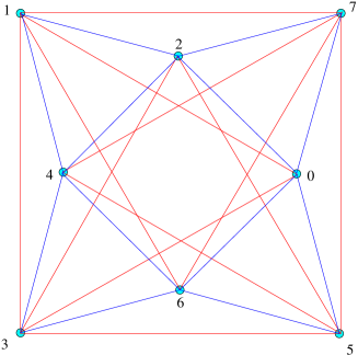
Figure 6: Another projection of the cross-polytope $\mathcal{O}$.

In Figure 6, each vertex of either of the two concentric squares forms an equilateral triangle with one edge of the other square. These $8$ triangles correspond to the unlabelled nodes in Figure 4, and also to the lines of the configuration $8_{3}$. (Any real triangle lies on a unique complex line in $\mathbb{C}^{2}$.) We may take the vertices in Figure 6 to be $(\pm 1,\pm 1)$ and $(\pm r,0),(0,\pm r)$, where $r=\sqrt{3}-1$.

But what plane $\Lambda$ in $\mathbb{E}^{4}$ actually gives such a projection? Starting with an unknown basis $a_{1},b_{1}$ for $\Lambda$, we can force a lot. For example, edge $[2,0]$ is the projection of $(0,2,-2,0)$ and is obtained from $[7,0]$, the projection of $(2,2,0,0)$, by a rotation through $60^{\circ}$. From such details in the geometry, we soon find that $\Lambda$ is uniquely determined and get a basis satisfying $a_{1}\cdot a_{1}=b_{1}\cdot b_{1}$ and $a_{1}\cdot b_{1}=0$. But any such basis can still be rescaled or rotated within $\Lambda$. Tweaking these finer details, we find it convenient to take $a_{1},b_{1}$ to be the first two rows of the matrix

$$L=\frac{1}{2\sqrt{3}}\left[\begin{array}[]{cccc}\sqrt{3}&-1&1&-(2+\sqrt{3})\\ -1&2+\sqrt{3}&\sqrt{3}&-1\\ -1&-\sqrt{3}&2+\sqrt{3}&1\\ 2+\sqrt{3}&1&1&\sqrt{3}\end{array}\right]\;.$$ (16)

The last two rows $a_{2},b_{2}$ of $L$ give a basis for the orthogonal complement $\Lambda^{\perp}$.

Since we want $J$ to induce $90^{\circ}$ rotations in both $\Lambda$ and $\Lambda^{\perp}$, we have

$$J=\frac{1}{\sqrt{3}}\left[\begin{array}[]{rrrr}0&1&-1&-1\\ -1&0&-1&1\\ 1&1&0&1\\ 1&-1&-1&0\end{array}\right]\;.$$ (17)

Notice that $a_{1}J=b_{1}$ and $a_{2}J=b_{2}$, so , $\{a_{1},a_{2}\}$ is a $\mathbb{C}$-basis for $\mathbb{E}^{4}$; and the plane $\Lambda$ in Figure 6 is just $z_{2}=0$ in the resulting complex coordinates. The points in the configuration $8_{3}$ now have these complex coordinates:

Label	$(z_{1},z_{2})$
$0$	$(r,1-\imath)$
$1$	$(-1+\imath,r)$
$2$	$(r\imath,-1-\imath)$
$3$	$(-1-\imath,-r\imath)$
$4$	$(-r,-1+\imath)$
$5$	$(1-\imath,-r)$
$6$	$(-r\imath,1+\imath)$
$0$	$(1+\imath,r\imath)$

(Recall that $r=\sqrt{3}-1$.) The first coordinates do give the points displayed in Figure 6. The second coordinates describe the projection onto $\Lambda^{\perp}$ ( $z_{1}=0$). There labels on the inner and outer squares are suitably swapped.

A typical line in the configuration $8_{3}$, like that containing points $1,6,7$, has equation

$$r(1-\imath)z_{1}+2z_{2}=2r(1+\imath)\;.$$

After consulting [7, Sections 10.6 and 11.2], we observe that the eight points are also the vertices of the regular complex polygon $3\{3\}3$. Its symmetry group (of unitary transformations on $\mathbb{C}^{2}$) is the group $3[3]3$ with the presentation

$$\langle\gamma_{1},\gamma_{2}\,|\,\gamma_{1}^{3}=1,\;\gamma_{1}\gamma_{2}\gamma_{1}=\gamma_{2}\gamma_{1}\gamma_{2}\rangle\;.$$ (18)

In fact, this group of order $24$ is isomorphic to the binary tetrahedral group $\langle 3,3,2\rangle$. But in our context, we may identify it with the centralizer in $G$ of the structure matrix $J$. A bit of computation shows that this subgroup of $G$ is generated by

$$\gamma_{1}=\rho_{1}\rho_{2}\rho_{3}\rho_{2}=(1,4,2)\;\mathrm{and}\;\gamma_{2}=\rho_{2}\rho_{0}\rho_{1}\rho_{0}=(-1,1,-1,1)\cdot(1,2,3),$$

which do satisfy the relations in (18).

Acknowledgements. I want to thank Daniel Pellicer, both for his many geometrical ideas and also for generously welcoming me to the Centro de Ciencias Matemáticas at UNAM (Morelia).

References

- [1] G. Araujo-Pardo, I. Hubard, D. Oliveros, and E. Schulte, Colorful Polytopes and Graphs, Israel Journal of Mathematics, 195 (2013), pp. 647–675.
- [2] N. Biggs, Algebraic Graph Theory, Cambridge University Press, Cambridge, UK, 2nd ed., 1993.
- [3] J. Bracho, I. Hubard, and D. Pellicer, A finite chiral 4-polytope in , Discrete Comput. Geom., 52 (2014), pp. 799–805.
- [4] H. S. M. Coxeter, Wythoff’s construction for uniform polytopes, Proc. London Math. Soc., 38 (1935), pp. 327–339. (Reprinted in The Beauty of Geometry: Twelve Essays, Dover, NY, 1999).
- [5] , Self-dual configurations and regular graphs, Bull. Amer. Math. Soc., 56 (1950), pp. 413–455.
- [6] , Regular Polytopes, Dover, New York, 3rd ed., 1973.
- [7] , Regular Complex Polytopes, Cambridge University Press, Cambridge, UK, 2nd ed., 1991.
- [8] H. S. M. Coxeter and W. O. J. Moser, Generators and Relations for Discrete Groups, Springer, New York, 3rd ed., 1972.
- [9] H. S. M. Coxeter and A. I. Weiss, Twisted Honeycombs and Their Groups, Geom. Dedicata, 17 (1984), pp. 169–179.
- [10] J. E. Humphreys, Reflection Groups and Coxeter Groups, Cambridge University Press, Cambridge, UK, 1990.
- [11] P. McMullen, Regular polytopes of full rank, Discrete Comput. Geom., 32 (2004), pp. 1–35.
- [12] P. McMullen, Geometric Regular Polytopes, vol. 172 of Encyclopedia of Mathematics and its Applications, Cambridge University Press, Cambridge, UK, 2020.
- [13] P. McMullen and E. Schulte, Abstract Regular Polytopes, vol. 92 of Encyclopedia of Mathematics and its Applications, Cambridge University Press, Cambridge, UK, 2002.
- [14] B. Monson, D. Pellicer, and G. Williams, Mixing and Monodromy of Abstract Polytopes, Trans. Amer. Math. Soc, 366 (2014), pp. 2651–2681.
- [15] D. Pellicer, Chiral polytopes of full rank exist only in ranks 4 and 5, Beitr. Algebra Geom., (2020).
- [16] E. Schulte and A. I. Weiss, Chiral polytopes, in Applied Geometry and Discrete Mathematics: The Victor Klee Festschrift, P. Gritzmann and B. Sturmfels, eds., vol. 4 of DIMACS Ser. Discrete Math. Theoret. Comput. Sci., Amer. Math. Soc., Assoc. Comput. Mach., 1991, pp. 493–516.
- [17] E. Schulte and A. I. Weiss, Chirality and projective linear groups, Discrete Math., 131 (1994), pp. 221–261.