Peeking into the $\theta$ vacuum

Abstract

We propose a subvolume method to study the $\theta$ dependence of the free energy density of the four-dimensional $\mathrm{SU}$($N$) Yang-Mills theory on the lattice. As an attempt, the method is first applied to $\mathrm{SU}$(2) Yang-Mills theory at $T=1.2\,T_{c}$ to understand the systematics of the method. We then proceed to the calculation of the vacuum energy density and obtain the $\theta$ dependence qualitatively different from the high temperature case. The numerical results combined with the theoretical requirements provide the evidence for the spontaneous CP violation at $\theta=\pi$, which is in accordance with the large $N$ prediction and indicates that the similarity between 4d SU($N$) and 2d CP${}^{N\!-\!1}$ theories does not hold for $N$=2.

I Introduction

The $\theta$ parameter of the 4d Yang-Mills theory controls relative weights of different topological sectors in the path integral. Despite long history, it still remains as a challenging problem to identify the effect of the $\theta$ parameter on the non-perturbative dynamics of the theory.

For the special value $\theta=\pi$ the Lagrangian has CP symmetry, and we can ask whether or not the CP symmetry is spontaneously broken. In the large $N$ limit tHooft:1973alw spontaneous CP violation at $\theta=\pi$ was demonstrated in Refs. Witten:1980sp ; tHooft:1981bkw ; Witten:1998uka . For finite $N$ a mixed anomaly between the CP symmetry and the $\mathbb{Z}_{N}$ center symmetry shows that the CP symmetry in the confining phase has to be broken Gaiotto:2017yup . A similar conclusion was derived by studying restoration of the equivalence of local observables in $\mathrm{SU}$($N$) and $\mathrm{SU}$($N$)/$\mathbb{Z}_{N}$ gauge theories in the infinite volume limit Kitano:2017jng . (See also Refs. Azcoiti:2003ai ; Yamazaki:2017dra ; Wan:2018zql .) While these theoretical developments have narrowed down possible scenarios, an explicit nonperturbative calculation is necessary to unambiguously settle the fate of the CP symmetry at $\theta=\pi$. Any direct numerical simulation at $\theta=\pi$, however, has been difficult due to the notorious sign problem .

In Ref. Kitano:2020mfk three of the authors of the present paper studied the vacuum energy density of the 4d $\mathrm{SU}$(2) Yang-Mills theory around $\theta=0$ by lattice numerical simulations. The case of $\mathrm{SU}$(2) gauge group is of particular interest since $N=2$ is farthest away from the large $N$ limit: there is a well-known parallel between 2d CP¹ and 4d $\mathrm{SU}$(2) model , and the known vacuum at $\theta=\pi$ in the former CP1 alludes to the appearance of gapless theory in the latter. By observing that the first two numerical coefficients in the $\theta$ expansion obey the large $N$ scaling , it was inferred in Ref. Kitano:2020mfk that the 4d $\mathrm{SU}$(2) Yang-Mills theory at $\theta=\pi$ has spontaneous CP breaking, contrary to the naive expectation from the 2d CP¹ model.

In this work, we develop a subvolume method to explore the $\theta$ dependence of the free energy without any series expansion in $\theta$ and apply to 4d $\mathrm{SU}$(2) theory. We find that it indeed works and show an evidence of spontaneous CP violation at $\theta=\pi$ at zero temperature, in consistency with the results of Ref. Kitano:2020mfk . The subvolume method here is inspired by Ref. Luscher:1978rn and similar to that introduced in Ref. KeithHynes:2008rw to study 2d CP${}^{N\!-\!1}$ model.

II Subvolume Method and Lattice Set Up

In what follows, the subvolume method is described. After generating a number of gauge configurations at $\theta=0$ and implementing the $n_{\rm APE}$ steps of APE smearing Albanese:1987ds , the topological charge density $q(x)$ is calculated with the five-loop improved topological charge operator deForcrand:1997esx on the lattice. Defining the subvolume topological charge $Q_{\rm sub}$,

$$Q_{\rm sub}=\displaystyle\sum_{x\in V_{\rm sub}}q(x)\ ,$$ (1)

we calculate the free energy density for the subvolume as Luscher:1978rn ; KeithHynes:2008rw ,

$$f_{\rm sub}(\theta)=\frac{-1}{V_{\rm sub}}\ln\frac{Z(\theta)}{Z(0)}=\frac{-1}{V_{\rm sub}}\ln\,\langle\,\cos\left(\theta\,Q_{\rm sub}\right)\,\rangle\ ,$$ (2)

$$Z(\theta)=\int\!\!{\cal D}U\,e^{-S_{g}+i\theta Q_{\rm sub}}\ ,$$ (3)

where $U$ denotes the link variable and $S_{g}$ the gauge action. Note that the expectation value $\langle\cdots\rangle$ is estimated on the $\theta=0$ configurations. The free energy density is then obtained as the infinite volume limit of $f_{\rm sub}(\theta)$:

$$f(\theta)=\lim_{V_{\rm sub}\to\infty}f_{\rm sub}(\theta)\ .$$ (4)

The goal of this study is to answer whether the spontaneous CP violation does occur at $\theta=\pi$. Thus, the order parameter should be useful and is calculated through

$$\frac{d\,f(\theta)}{d\,\theta}=\lim_{V_{\rm sub}\rightarrow\infty}\frac{d\,f_{\rm sub}(\theta)}{d\,\theta}\ ,$$ (5)

$$\frac{d\,f_{\rm sub}(\theta)}{d\,\theta}=\frac{1}{V_{\rm sub}}\frac{\left\langle Q_{\rm sub}\,\sin(\theta Q_{\rm sub})\right\rangle}{\langle\,\cos(\theta Q_{\rm sub})\,\rangle}\,.$$ (6)

$f$ and $df/d\theta$ are evaluated separately and later used to make a consistency check.

Some cautions are in order. First, the size of the subvolume $V_{\rm sub}$ cannot be arbitrary. Obviously it has to be large enough to cover the typical correlation length of the system, which is considered to be around $1/(aT_{c})=9.50$ Giudice:2017dor in the lattice unit. We thus restrict the size of the subvolume to $V_{\rm sub}\geq 10^{4}$. Suppose that $V_{\rm sub}$ is large enough but $V_{\rm sub}\ll V_{\rm full}$, where $V_{\rm full}$ denotes the full volume. Then, the resulting $f(\theta)$ is expected to be independent of $V_{\rm full}$, and $f_{\rm sub}$ would shows a scaling behavior as a function of $V_{\rm sub}$. As $V_{\rm sub}$ grows and approaches $V_{\rm full}$, $Q_{\rm sub}$ becomes close to an integer global $Q$, and $f_{\rm sub}$ starts to converge a full volume result, in which we are not interested as it becomes clear later. The critical goal in this method is to identify the scaling behavior from which the infinite volume limit is extracted.

Secondly, the observables (2) and (6) contain the expectation value $\langle\cos(\theta Q_{\rm sub})\rangle$. Either observable becomes incalculable when $\langle\cos(\theta Q_{\rm sub})\rangle$ fluctuates across zero. This is the sign problem in this method and sets the $\theta$ dependent upper limit on the size of $V_{\rm sub}$. Thus, another crucial point is whether the scaling behavior is realized before $V_{\rm sub}$ reaches the upper limit. We will return to this point in the discussion section.

The free energy density of 4d $\mathrm{SU}$(2) Yang-Mills theory is calculated at high and zero temperatures below. We employ the configurations generated in our previous work at $T=0$ Kitano:2020mfk , while the ensemble corresponding to $T=1.2\,T_{c}$ is newly generated at the lattice coupling $\beta=1.975$, the same as the $T=0$ case. The simulation parameters are summarized in Tab. 1.

$N_{S}^{3}\times N_{T}$	$T/T_{c}$	[${n_{\rm APE}}_{\rm min},\ {n_{\rm APE}}_{\rm max}$]	statistics	$a^{4}\chi\times 10^{5}$
$24^{3}\times 8$	1.21	[25, 45]	10,000	1.35(5)
$24^{3}\times 48$	0	[20, 40]	68,000	2.54(3)

Table 1: The lattice parameters of the ensembles. The tree-level Symanzik improved action Weisz:1982zw is adopted with the periodic boundary conditions in all four directions. The value $1/(aT_{c})=9.50$ Giudice:2017dor gives the value of $T/T_{c}$ in the table, where $T_{c}$ is the critical temperature at $\theta=0$.

The topological charge density measured at each smearing step is uniformly shifted as $q(x)\to q(x)+\epsilon$ at every configurations so that the global topological charge $Q=\sum_{x\in V_{\rm full}}q(x)$ takes the integer closest to the original value. The calculation of $Q_{\rm sub}$ is carried out every five smearing steps. For the APE smearing, we take $\alpha=0.6$ in the notation of Ref. Alexandrou:2017hqw .

Topological observables on the lattice can be distorted by topological lumps originating from lattice artifacts. One can take away those by the smearing procedure, but at the same time the smearing may deform physical topological excitations, too. We studied this point in detail in Ref. Kitano:2020mfk , and developed the procedure to restore the physical information. The procedure consists of the extrapolation of the observables to the zero smearing limit by fitting over a suitable interval of the smearing steps. The fit range is fixed in advance by examining the response of the global topological charge to the smearing as done in Ref. Kitano:2020mfk . The resulting fit ranges and the topological susceptibilities $\chi=\langle\,Q^{2}\,\rangle/V_{\rm full}$ thus determined using the global topological charge $Q$ are shown in Tab. 1 for later use.

The $\theta$-dependence is explored in the range of $\theta=k\,\pi/10$ with $k\in[1,\,20]$. Each configuration is separated by ten Hybrid Monte Carlo (HMC) trajectories. In the following analysis, statistical errors are estimated by the single-elimination jack-knife method with the bin size of 500 and 100 configurations for zero and high temperatures, respectively. We mainly show the analysis of $f(\theta)$, but $df(\theta)/d\theta$ is analyzed in parallel with similar quality.

III Testing the method at High Temperature

We first apply the subvolume method to the calculation of the free energy density above $T_{c}$, where the instanton prediction, $f(\theta)\sim\chi(1-\cos\theta)$ 'tHooft:1976fv ; Callan:1977gz ; Gross:1980br , is believed to be valid and numerically supported for $\mathrm{SU}$($N$) with $N\geq 3$ Bonati:2013tt ; Frison:2016vuc as well. Using the translational invariance, a single-sized subvolume $V_{\rm sub}/a^{4}=l^{3}\times N_{T}$ with $l=10,\ 12,\ \cdots,\ 24$ is taken from 64 places per a configuration, and the results are averaged.

The $l$ dependence of $f_{\rm sub}$ is shown in Fig. 1.

Figure 1: The subvolume dependence of $f_{\rm sub}(\theta)$ and the extrapolation to the infinite volume limit.

It is found that in general the measured $l$ dependence is not constant and the leading correction linear in $1/l$ is inevitable. The linear dependence is seen for $\theta=\pi/2$ for $l\leq 22$, whereas it ends around $l=20$ for $\theta=\pi$ and it is hard to determine the linear region for $\theta=3\pi/2$. Thus, it turns out to be difficult to identify the scaling region unambiguously especially when $\theta$ is large, and hence we give up the precise determination. Instead, we choose three fit ranges in each extrapolation and try to estimate the potential size of the systematic uncertainty due to the ambiguity of the scaling region. Three fit ranges, $l\in[12,16]$, $[14,18]$ and $[16,20]$, are examined when fitting to the expected scaling behavior

$$f_{\rm sub}(\theta)=f(\theta)+\frac{a^{-1}\,s(\theta)}{l}\,,$$ (7)

where $s(\theta)$ denotes the surface tension of the nonzero $\theta$ domain and $a$ the lattice spacing. All fits performed in this analysis yield $\chi^{2}/\mbox{dof}<3$. It is interesting to see that the relative relation $f_{\rm sub}(3\pi/2)>f_{\rm sub}(\pi)$ at small $l$ flips toward the large $l$ limit and $f(\theta)$ ends up with non-monotonic function. Since the data of $f_{\rm sub}$ smoothly (but sometimes rapidly) connect the full volume ($l^{3}\times 6=24^{3}\times 6$) results from the above, the extrapolation fitting the data near the full volume tends to be smaller than that fitting the data far from the full volume. As a result, the discrepancy, i.e. the potential size of the systematic uncertainty, turns out to be larger at larger $\theta$.

The results thus obtained are then extrapolated to $n_{\rm APE}=0$ at each value of $\theta$ with the fit range shown in Tab. 1. In the extrapolation, the linear fit goes well with $\chi^{2}/\mbox{dof}<3$. The stability against small shifts of the fit range is seen in Fig. 2.

Figure 2: The linear extrapolation of $f(\theta)$ to $n_{\rm APE}=0$, where $f(\theta)$ is obtained by the fit with $l\in[14,18]$.

Finally, the free energy density obtained with three fit ranges are shown in Fig. 3 together with the full volume result (filled squares), where $f(\theta)$ is normalized by the topological susceptibility in Tab. 1.

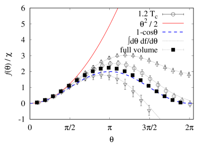
Figure 3: The $\theta$ dependence of $f(\theta)$ at $T=1.2\,T_{c}$. The results obtained with different fit ranges in Fig. 1, $l\in[12,16]$, $[14,18]$ and $[16,20]$, are shown in triangle-up, circle and triangle-down, respectively.

The prediction from the dilute instanton gas approximation, $1-\cos(\theta)$, is shown by the dashed curve. The function, $\theta^{2}/2$, is also shown as the solid curve for comparison. Taking into account the uncertainty arising from the ambiguity of the scaling region, the numerical results are consistent with the instanton prediction. Note that non-monotonic behavior of $f(\theta)$ seems robust at high temperature but is far from obvious before the extrapolations, as the surface tension term in Eq. (7) is monotonic.

$f(\theta)$ can also be obtained from the numerical integration of $df(\theta)/d\theta$ as shown by the dotted curves. The agreement with those curves supports that the two nontrivial extrapolations included in the whole analysis do not pick up accidental fluctuations and are stable.

The result with full volume is found to well agree with the instanton prediction. One may think that this is the simplest way to obtain $f(\theta)$. However, we will see that it does not work at $T=0$. From the test, assuming that the instanton prediction is valid at high temperature, we learn that the scaling behavior of $f_{\rm sub}$ would be linear and the region showing such a behavior starts around the dynamical length scale ($\sim 1/(aT_{c})$).

IV Applying to Zero Temperature

Next we apply the subvolume method to calculate the vacuum energy density. This time the subvolume is defined by $V_{\rm sub}/a^{4}=l^{4}$ with $l=10,12,\ \cdots,\ 24$ and taken from 512 places per configuration. The $l$ dependence of $f_{\rm sub}(\theta)$ is shown in Fig. 4 as before.

Figure 4: The linear extrapolation of $f_{\rm sub}(\theta)$ to the infinite volume limit.

Due to the sign problem in this method, some results at large $\theta$ and large $l$ could not be calculated. But the available data show linear behavior. Following the previous analysis, three fit ranges of $l\in[10,14]$, $[12,16]$ and $[14,18]$ are taken in the fit to (7) to estimate the systematic uncertainty. Contrary to the high temperature case, $f(\theta)$ turns out to be stable against the variation of the fit range, and does not show any sign of the flip, indicating monotonic behaviors of $f(\theta)$ as a function of $\theta$.

The linear extrapolation to $n_{\rm APE}=0$ is carried out with the fit range shown in Tab. 1, and the fit is found to work well with $\chi^{2}/$dof $<3$ as shown in Fig. 5.

Figure 5: The linear extrapolation of $a^{4}f(\theta)$ to $n_{\rm APE}=0$ for the data obtained with $l\in[12,16]$.

The stability against shift of the fit range is also confirmed.

Finally, the resulting $f(\theta)$ and $df(\theta)/d\theta$ are shown in Fig. 6 together with the predictions from the large $N$ ($\theta^{2}/2$) and the instanton calculus ($1-\cos\theta$).

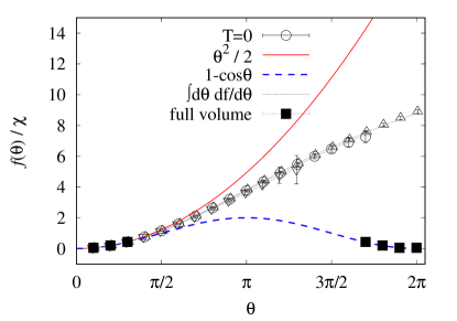
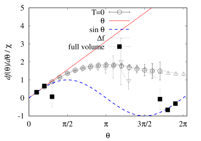
Figure 6: $f(\theta)$ (top) and $df(\theta)/d\theta$ (bottom). The results obtained with different fit ranges in Fig. 4, $l\in[10,14]$, $[12,16]$ and $[14,18]$, are shown in triangle-up, circle and triangle-down, respectively.

The stability of the two extrapolations during the analysis is confirmed as $f(\theta)$ and $df(\theta)/d\theta$ well agree with the dotted curves. While the full volume calculation works only in the vicinity of $\theta=0$, the subvolume method succeeds to calculate, at least, to $\theta\sim\pi$. There are crucial differences from the high temperature case. First, the different choices of the fit range in $l$ yield consistent results, and hence the potential systematic error from the ambiguity of the scaling region seems to be under control. Second, $f(\theta)$ is a monotonically increasing function, at least, to $\theta\sim\pi$, and the direct calculation of $df(\theta)/d\theta$ clearly shows $d\,f(\theta)/d\theta|_{\theta=\pi}\neq 0$. Since $d\,f(\theta)/d\theta=-i\langle q(x)\rangle$ is CP odd, we conclude that CP is spontaneously broken at $\theta=\pi$ in the vacuum of the 4d $\mathrm{SU}$(2) Yang-Mills theory  and that there is a phase transition to recover the CP symmetry at some finite temperature. In other words, it is found that the 4d SU(2) Yang-Mills theory is in the large-$N$ class unlike the 2d CP¹ model .

V Discussion

The symmetry of $\mathrm{SU}$($N$) gauge theories indicates $f(\theta)=f(-\theta)$ and $f(\theta)=f(\theta+2\pi)$. In the subvolume method, $f(\theta)=f(-\theta)$ is automatic from (2) but the $2\pi$-periodicity is not seen in $f(\theta)$ shown in Fig. 6.

The subvolume method is equivalent to modifying the value of $\theta$ inside the subvolume. If the difference of $\theta$ is a multiple of $2\pi$ and the calculation respects the $2\pi$-periodicity, the free energy would scale as the surface area of the subvolume when the subvolume is large enough. The lack of $2\pi$ periodicity in the free energy density should thus be interpreted as the presence of a meta-stable vacuum for a fixed value of $\theta$ (except for $\theta=\pi$ where two vacua interchanged by CP are degenerate and stable). Thus, we expect that the meta-stable vacuum should eventually decay into the stable one by the creation of a dynamical domain wall that attaches to the interface.

The absence of the decay of the domain into the domain-wall in the lattice calculation has an analog in the calculation of the static potential . The static potential is calculated by inserting a Wilson loop, and should show the string breaking for configurations with light dynamical quarks when the two test charges are distant enough. But it does not occur, at least, within naive methods, and the resulting potential sticks to the original branch even after passing the transition point. The probable reason is that the overlap between the original state with two static charges and another lower energy state with two mesons are extremely small. We infer that the same happens to the calculation of $f(\theta)$ for $\theta>\pi$ and the first order phase transition is missing . It is clearly interesting to directly see the formation of the domain wall on the lattice though it would not be straightforward.

We have mentioned the $\theta$ dependent upper limit on the size of $V_{\rm sub}$ in sec. II. We examine the relation between the limit and $\theta\langle|Q_{\rm sub}|\rangle$ at $T=0$. Figure 7 shows $\theta\langle|Q_{\rm sub}|\rangle$ as a function of $1/l$, where we have used the approximate relation $\langle|Q_{\rm sub}|\rangle=(l^{4}/V_{\rm full})^{1/2}\langle|Q|\rangle$ and the measured value of $\langle|Q|\rangle$ at $T=0$ by ignoring the corrections to the relation of $O(1/l)$ and $O(1/(\chi V_{\rm sub}))$.

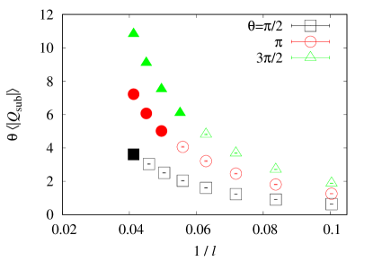
Figure 7: Subvolume dependence of $\theta\langle\,|Q_{\rm sub}|\,\rangle$. The open symbols represent the calculations which succeeded while the filled ones represent those which failed.

In the figure, the filled symbols represent the points where the calculations are failed due to the sign problem. It is seen that the upper limit indeed decreases with $\theta$. Numerical investigation suggests that the upper limit on the subvolume scales as $1/\theta$.

VI Summary

We developed the subvolume method, which enables us to extract the $\theta$ dependence of the free energy density in 4d Yang-Mills theory not restricted to $\theta\sim 0$. At high temperature, the method yields $\theta$ dependence consistent with the instanton prediction, as expected, within the large uncertainty due to the ambiguity of the scaling region. To fix this ambiguity, it is necessary to go to larger lattices. On the other hand, at zero temperature the sign problem arises instead, but still $f(\theta)$ could be calculated to $\theta\sim\pi$ with the systematic uncertainty under control. Combining the numerical result with the theoretical requirement leads to the conclusion that the vacuum of 4d $\mathrm{SU}$(2) Yang-Mills theory undergoes spontaneous CP violation at $\theta=\pi$ as large $N$ theory does. Although the overlap problem prohibits the domain-wall from being formed, it is interesting to learn that such a object actually exists in the Yang-Mills theory Luscher:1978rn .

We have tested the stability of the results by exchanging the order of extrapolations and obtained the consistent results with enlarged uncertainties.

In order to promote this study to the quantitative level, it is necessary to perform lattice simulations with larger volumes and finer lattice spacings. Further studies will be presented in the forthcoming paper InProgress . It is a fascinating question to ask if our method is applicable for other questions with sign problems, such as gauge theories with finite values of the chemical potential.

While numerical results are not accurate past $\theta\sim 3\pi/2$, there are indications that the derivative $df(\theta)/d\theta$ decreases past $\theta=\pi$, and becomes smaller near $\theta\sim 2\pi$. This is consistent with the expectation Yamazaki:2017ulc that there are two meta-stable branches of the $\mathrm{SU}$(2) theory, each of which has $4\pi$ periodicity.

References

- (1) G. ’t Hooft, Nucl. Phys. B 72, 461 (1974)
- (2) E. Witten, Annals Phys. 128, 363 (1980)
- (3) G. ’t Hooft, Nucl. Phys. B 190, 455-478 (1981)
- (4) E. Witten, Phys. Rev. Lett. 81, 2862-2865 (1998) [arXiv:hep-th/9807109 [hep-th]].
- (5) D. Gaiotto, A. Kapustin, Z. Komargodski and N. Seiberg, JHEP 05, 091 (2017) [arXiv:1703.00501 [hep-th]].
- (6) R. Kitano, T. Suyama and N. Yamada, JHEP 09, 137 (2017) [arXiv:1709.04225 [hep-th]].
- (7) V. Azcoiti, A. Galante and V. Laliena, Prog. Theor. Phys. 109, 843-851 (2003) [arXiv:hep-th/0305065 [hep-th]].
- (8) M. Yamazaki, JHEP 10, 172 (2018) [arXiv:1711.04360 [hep-th]].
- (9) Z. Wan, J. Wang and Y. Zheng, Annals Phys. 414, 168074 (2020) [arXiv:1812.11968 [hep-th]].
- (10) M. Hirasawa, A. Matsumoto, J. Nishimura and A. Yosprakob, JHEP 09, 023 (2020) [arXiv:2004.13982 [hep-lat]].
- (11) C. Gattringer and O. Orasch, Nucl. Phys. B 957, 115097 (2020) [arXiv:2004.03837 [hep-lat]].
- (12) R. Kitano, N. Yamada and M. Yamazaki, JHEP 2021, 73 (2021), [arXiv:2010.08810 [hep-lat]].
- (13) M. Yamazaki and K. Yonekura, JHEP 07, 088 (2017) [arXiv:1704.05852 [hep-th]].
- (14) F. D. M. Haldane, Phys. Rev. Lett. 50, 1153-1156 (1983); F. D. M. Haldane, Phys. Lett. A 93, 464-468 (1983); I. Affleck and F. D. M. Haldane, Phys. Rev. B 36, 5291-5300 (1987); R. Shankar and N. Read, Nucl. Phys. B 336, 457-474 (1990); I. Affleck, Phys. Rev. Lett. 66, 2429-2432 (1991); A. B. Zamolodchikov and A. B. Zamolodchikov, Nucl. Phys. B 379, 602-623 (1992); W. Bietenholz, A. Pochinsky and U. J. Wiese, Phys. Rev. Lett. 75, 4524-4527 (1995); B. Alles and A. Papa, Phys. Rev. D 77, 056008 (2008); [arXiv:0711.1496 [cond-mat.stat-mech]]; B. Alles, M. Giordano and A. Papa, Phys. Rev. B 90, no.18, 184421 (2014) [arXiv:1409.1704 [hep-lat]].
- (15) B. Lucini and M. Teper, JHEP 06, 050 (2001) [arXiv:hep-lat/0103027 [hep-lat]].
- (16) L. Del Debbio, H. Panagopoulos and E. Vicari, JHEP 08, 044 (2002) [arXiv:hep-th/0204125 [hep-th]].
- (17) C. Bonati, M. D’Elia, P. Rossi and E. Vicari, Phys. Rev. D 94, no. 8, 085017 (2016) [arXiv:1607.06360 [hep-lat]].
- (18) P. de Forcrand, M. Garcia Perez and I. O. Stamatescu, Nucl. Phys. B 499, 409 (1997) [hep-lat/9701012].
- (19) T. A. DeGrand, A. Hasenfratz and T. G. Kovacs, Nucl. Phys. B 505, 417-441 (1997) [arXiv:hep-lat/9705009 [hep-lat]].
- (20) B. Alles, M. D’Elia and A. Di Giacomo, Phys. Lett. B 412, 119-124 (1997) [arXiv:hep-lat/9706016 [hep-lat]].
- (21) B. A. Berg and D. A. Clarke, Phys. Rev. D 97, no.5, 054506 (2018) [arXiv:1710.09474 [hep-lat]].
- (22) M. Luscher, Phys. Lett. B 78, 465-467 (1978)
- (23) P. Keith-Hynes and H. Thacker, Phys. Rev. D 78, 025009 (2008) [arXiv:0804.1534 [hep-lat]].
- (24) M. Albanese et al. [APE], Phys. Lett. B 192, 163-169 (1987)
- (25) P. Giudice and S. Piemonte, Eur. Phys. J. C 77, no.12, 821 (2017) [arXiv:1708.01216 [hep-lat]].
- (26) P. Weisz, Nucl. Phys. B 212, 1-17 (1983).
- (27) C. Alexandrou, A. Athenodorou, K. Cichy, A. Dromard, E. Garcia-Ramos, K. Jansen, U. Wenger and F. Zimmermann, Eur. Phys. J. C 80, no.5, 424 (2020) [arXiv:1708.00696 [hep-lat]].
- (28) G. ’t Hooft, Phys. Rev. D 14, 3432 (1976) [Phys. Rev. D 18, 2199 (1978)].
- (29) C. G. Callan, Jr., R. F. Dashen and D. J. Gross, Phys. Rev. D 17, 2717 (1978)
- (30) D. J. Gross, R. D. Pisarski and L. G. Yaffe, Rev. Mod. Phys. 53, 43 (1981)
- (31) C. Bonati, M. D’Elia, H. Panagopoulos and E. Vicari, Phys. Rev. Lett. 110, no.25, 252003 (2013) [arXiv:1301.7640 [hep-lat]].
- (32) J. Frison, R. Kitano, H. Matsufuru, S. Mori and N. Yamada, JHEP 09, 021 (2016) doi:10.1007/JHEP09(2016)021 [arXiv:1606.07175 [hep-lat]].
- (33) M. Unsal, Phys. Rev. D 86, 105012 (2012) [arXiv:1201.6426 [hep-th]].
- (34) M. Ünsal, [arXiv:2007.03880 [hep-th]].
- (35) R. Kitano, R. Matsudo, N. Yamada and M. Yamazaki, in progress.
- (36) S. Ueda, S. Aoki, T. Aoyama, K. Kanaya, H. Matsufuru, S. Motoki, Y. Namekawa, H. Nemura, Y. Taniguchi and N. Ukita, J. Phys. Conf. Ser. 523, 012046 (2014)