Doubly hidden $0^{++}$ molecules and tetraquarks states from QCD at NLO

Abstract

Motivated by the LHCb-group discovery of exotic hadrons in the range (6.2 $\sim$ 6.9) GeV, we present new results for the masses and couplings of $0^{++}$ fully heavy $(\bar{Q}Q)(Q\bar{Q})$ molecules and $(QQ)(\overline{QQ})$ tetraquaks states from relativistic QCD Laplace Sum Rule (LSR) within stability criteria where Next-to-Leading Order (NLO) Factorized (F) Perturbative (PT) corrections is included. As the Operator Product Expansion (OPE) usually converges for $d\leqslant 6-8$, we evaluated the QCD spectral functions at Lowest Order (LO) of PT QCD and up to $\langle G^{3}\rangle$. We also emphasize the importance of PT radiative corrections for heavy quark sum rules in order to justify the use of the running heavy quark mass value in the analysis. We compare our predictions in Table 3 with the ones from ratio of Moments (MOM). The broad structure arround (6.2 $\sim$ 6.9) GeV can be described by the $\overline{\eta}_{c}\eta_{c}$, $\overline{J/\psi}J/\psi$ and $\overline{\chi}_{c1}\chi_{c1}$ molecules or/and $\overline{S}_{c}S_{c}$, $\overline{A}_{c}A_{c}$ and $\overline{V}_{c}V_{c}$ tetraquarks lowest mass ground states. The narrow structure at (6.8 $\sim$ 6.9) GeV if it is a $0^{++}$ state can be a $\overline{\chi}_{c0}\chi_{c0}$ molecules or/and its analogue $\overline{P}_{c}P_{c}$ tetraquark. The $\overline{\chi}_{c1}\chi_{c1}$ predicted mass is found to be below the $\chi_{c1}\chi_{c1}$ threshold while for the beauty states, all of the estimated masses are above the $\eta_{b}\eta_{b}$ and $\Upsilon(1S)\Upsilon(1S)$ threshold.

1 Introduction

Recently, the LHCb collaboration [1, 2] studied the $J/\psi$-pair invariant mass spectrum and observed a narrow structure at $6.9$ GeV and a bump around $(6.2\sim 6.7)$ GeV as we can see in Fig. 1. In Ref. [3], which we partly review here, we use the inverse Laplace Transform (LSR) [4, 5, 6, 7, 8] of QCD spectral sum rules (QSSR) to estimate the masses and couplings of $0^{++}$ fully heavy molecules and tetraquarks states for interpreting these recent experimental data. In so doing, we include the NLO PT corrections from factorized part diagrams which is a good approximation as we shall see that the contribution from Non-Factorized (NF) diagrams is almost negligible compared to the total $\alpha_{s}$ contributions. This feature has been already observed explicitly in our previous works [20, 21, 22, 23]. We evaluate the four-quark correlators at LO of PT QCD up to the triple gluon condensate.

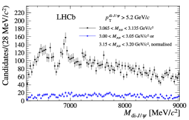
Figure 1: Ivariant mass spectrum of $J/\psi$-pair candidate. Data (resp. background regions) in black (resp. blue) signal[1].

2 The Laplace sum rule

We shall work with the finite energy version of the QCD inverse Laplace sum rules and their ratios:

$$\mathcal{L}^{c}_{n}(\tau,\mu) = \int^{t_{c}}_{16m^{2}_{Q}}dt\,t^{n}e^{-t\tau}\frac{1}{\pi}\mbox{Im}\Pi^{H}_{\mathcal{M},\mathcal{T}}(t,\mu),$$

$$\mathcal{R}^{c}_{n}(\tau) = \frac{\mathcal{L}^{c}_{n+1}}{\mathcal{L}^{c}_{n}},$$ (1)

where $m_{Q}$ is the heavy quark mass, $\tau$ is the LSR variable, $n=0,1$ is the degree of moments, $t_{c}$ is the ”QCD continuum” which parametrizes, from the discontinuity of the Feynman diagrams, the spectral function $\mbox{Im}\Pi^{S}_{\mathcal{M},\mathcal{T}}(t,m^{2}_{Q},\mu^{2})$ where $\Pi^{S}_{\mathcal{M},\mathcal{T}}(t,m^{2}_{Q},\mu^{2})$ is the scalar correlator defined as:

$$\Pi^{S}_{\mathcal{M},\mathcal{T}}(q^{2})=\int d^{4}x\,e^{-iqx}\langle 0|\mathcal{T}\mathcal{O}^{S}_{\mathcal{M},\mathcal{T}}(x)(\mathcal{O}^{S}_{\mathcal{M},\mathcal{T}}(x))^{{\dagger}}|0\rangle,$$ (2)

where $\mathcal{O}^{S}_{\mathcal{M},\mathcal{T}}(x)$ are the interpolating currents for the molecule $\mathcal{M}$ and tetraquark $\mathcal{T}$ states. The superscript $S$ refers to the spin of the scalar particles.

3 Interpolating currents

We shall be concerned with the interpolating currents given in Eq. 3 and Table 1.

$$\mathcal{O}^{S}_{\mathcal{T}}=\epsilon_{abc}\,\epsilon_{dec}\,(Q^{T}_{a}\,C\,\gamma_{\mu}\,Q_{b})(\bar{Q}_{d}\,\gamma^{\mu}\,C\,\bar{Q}^{T}_{e})$$ (3)

Table 1: Interpolating currents $\mathcal{O}^{S}_{\mathcal{M},\mathcal{T}}$ with a definite C-parity describing the molecules and tetraquarks states. $Q,q\equiv c,b$

Scalar States ($0^{++}$)	Current ($\mathcal{O}^{S}_{\mathcal{M},\mathcal{T}}$)
Molecules
$\overline{\chi}_{q0}\,\chi_{q0}$	$(\bar{Q}\,Q)(\bar{Q}\,Q)$
$\overline{\eta}_{q}\,\eta_{q}$	$(\bar{Q}\,\gamma_{5}\,Q)(\bar{Q}\,\gamma_{5}\,Q)$
$\overline{J/\psi}\,J/\psi$, $\overline{\Upsilon}\,\Upsilon$	$(\bar{Q}\,\gamma_{\mu}\,Q)(\bar{Q}\,\gamma^{\mu}\,Q)$
$\overline{\chi}_{q1}\,\chi_{q1}$	$(\bar{Q}\,\gamma_{\mu}\gamma_{5}\,Q)(\bar{Q}\,\gamma^{\mu}\gamma_{5}\,Q)$
Tetraquarks
$\overline{P}_{q}\,P_{q}$	$(Q^{T}_{a}\,C\,Q_{b})(\bar{Q}_{a}\,C\,\bar{Q}^{T}_{b})$
$\overline{S}_{q}\,S_{q}$	$(Q^{T}_{a}\,C\,\gamma_{5}Q_{b})(\bar{Q}_{a}\,\gamma_{5}\,C\,\bar{Q}^{T}_{b})$
$\overline{A}_{q}\,A_{q}$	$(Q^{T}_{a}\,C\,\gamma_{\mu}\,Q_{b})(\bar{Q}_{a}\,\gamma^{\mu}\,C\,\bar{Q}^{T}_{b})$
$\overline{V}_{q}\,V_{q}$	$(Q^{T}_{a}\,C\,\gamma_{\mu}\gamma_{5}\,Q_{b})(\bar{Q}_{a}\,\gamma^{\mu}\gamma_{5}\,C\,\bar{Q}^{T}_{b})$

4 The Spectral function

We shall use the Minimal Duality Ansatz (MDA) for parametrizing the molecule spectral function:

$$\frac{1}{\pi}\mbox{Im}\Pi^{S}_{\cal{M}}\simeq f^{2}_{\cal{M}}M^{8}_{\cal{M}}\delta(t-M_{\cal{M}}^{2})+\mbox{"QCD continuum"}\theta(t-t_{c}),$$ (4)

where the ”QCD continuum” is the imaginary part of the QCD correlator from the threshold $t_{c}$. The decay constant $f_{\cal{M}}$ (analogue to $f_{\pi}$) for the molecule state is defined as:

$$\langle 0|\mathcal{O}^{S}_{\mathcal{M}}|\mathcal{M}\rangle=f^{S}_{\mathcal{M}}\,M^{4}_{\mathcal{M}}.$$ (5)

Interpolating currents constructed from bilinear (pseudo)scalar currents are not renormalization group invariants such that the corresponding decay constants possess anomalous dimension:

$$f^{S}_{\mathcal{M}}(\mu)=\hat{f}^{S}_{\mathcal{M}}(-\beta_{1}\,a_{s})^{4/\beta_{1}}(1-k_{f}\,a_{s}),$$ (6)

where $\hat{f}^{S}_{\mathcal{M}}$ is the renormalization group invariant coupling and $[-\beta_{1}=(1/2)(11-2n_{f}/3)]$ is the first coefficient of the QCD $\beta$-function for $n_{f}$ flavors. $a_{s}\equiv(\alpha_{s}/\pi)$ is the QCD coupling. $k_{f}=2.028(2.352)$ for $n_{f}=4(5)$ flavors.
Within such a parametrization, one obtains:

$$\mathcal{R}^{c}_{0}\equiv\mathcal{R}\simeq M^{2}_{\mathcal{M}},$$ (7)

where $M_{\mathcal{M}}$ is the lowest ground state mass. Analogous definitions can be obtained for the tetraquark states by changing the subscripts $\mathcal{M}$ into $\mathcal{T}$.

5 NLO PT corrections and stability criteria

Assuming a factorization of the four-quark interpolating current, we can write the corresponding spectral function as a convolution of the two ones associated to two quark bilinear currents. In this way, we obtain [24, 25]:

$$\frac{1}{\pi}{\rm Im}\Pi^{H}_{\mathcal{M},\,\mathcal{T}}(t) = \theta(t-16M_{Q}^{2})\left(\frac{k}{4\pi}\right)^{2}t^{2}\int_{4m_{Q}^{2}}^{(\sqrt{t}-2m_{Q})^{2}}dt_{1}$$ (8)

$$\times\int_{4m_{Q}^{2}}^{(\sqrt{t}-\sqrt{t_{1}})^{2}}dt_{2}\,\lambda^{1/2}\,\mathcal{K}^{H},$$

where $k$ is an appropriate normalization factor, $m_{Q}$ the on-shell heavy quark mass and

$$\mathcal{K}^{S,P} \equiv \left(\frac{t_{1}}{t}+\frac{t_{2}}{t}-1\right)^{2}\times\frac{1}{\pi}{\rm Im}\psi^{S,P}(t_{1})\frac{1}{\pi}{\rm Im}\psi^{S,P}(t_{2})\,,$$ (9)

$$\mathcal{K}^{V,A} \equiv \left[\left(\frac{t_{1}}{t}+\frac{t_{2}}{t}-1\right)^{2}+\frac{8t_{1}t_{2}}{t^{2}}\right]\times\frac{1}{\pi}{\rm Im}\Pi^{V,A}(t_{1})\frac{1}{\pi}{\rm Im}\Pi^{V,A}(t_{2})\,,$$

with the phase space factor:

$$\lambda=\left(1-\frac{\left(\sqrt{t_{1}}-\sqrt{t_{2}}\right)^{2}}{t}\right)\left(1-\frac{\left(\sqrt{t_{1}}+\sqrt{t_{2}}\right)^{2}}{t}\right)~{}.$$ (10)

The NLO expressions of the spectral functions of the bilinear equal masses (pseudo)scalar and (axial-)vector are known in the literature [11, 12, 17, 26].
The variables $\tau,\mu$ and $t_{c}$ are, in principle, free external parameters. We shall use stability criteria with respect to these free 3 parameters to extract the lowest ground state mass and coupling (more detailed discussions can be seen in [20, 21, 22, 23, 27, 28, 29, 30] and references therein).

6 The On-shell and $\overline{\mbox{MS}}$-scheme

In our analysis, we replace the on-shell (pole) masses $m_{Q}$ appearing in the spectral functions with the running masses $\overline{m}_{Q}(\mu)$ using the relation, to order $\alpha^{2}_{s}$ [31, 32, 33, 34]:

$$m_{Q} = \overline{m}_{Q}(\mu)\Big{[}1+\frac{4}{3}a_{s}+(16.2163-1.0414n_{l})a_{s}^{2}$$ (11)

$$+\mbox{Log}{\left(\frac{\mu}{m_{Q}}\right)^{2}}\left(a_{s}+(8.8472-0.3611n_{l})a_{s}^{2}\right)$$

$$+\mbox{Log}^{2}{\left(\frac{\mu}{m_{Q}}\right)^{2}}\left(1.7917-0.0833n_{l}\right)a_{s}^{2}...\Big{]},$$

for $n_{l}$ light flavours where $\mu$ is the arbitrary subtraction scale.

7 QCD input parameters

The QCD parameters which shall appear in the following analysis will be the QCD coupling $\alpha_{s}$, the charm and bottom quark masses $m_{c,b}$, the gluon condensates $\langle\alpha_{s}G^{2}\rangle\equiv\langle\alpha_{s}G^{a}_{\mu\nu}G_{a}^{\mu\nu}\rangle$ and $\langle g^{3}G^{3}\rangle\equiv\langle g^{3}f_{abc}G^{a}_{\mu\nu}G^{b}_{\nu\rho}G^{c}_{\rho\mu}\rangle$. Their values are given in Table 2.

Table 2: QCD input parameters from recent QSSR analysis based on stability criteria.

Parameters	Values	Sources	Ref.
$\alpha_{s}(M_{Z})$	$0.1181(16)(3)$	$M_{\chi_{0c,b}}-M_{\eta_{c,b}}$	LSR [35]
$\overline{m}_{c}(\overline{m}_{c})$	$1286(16)$ MeV	$B_{c}\oplus J/\psi$	Mom [36]
$\overline{m}_{b}(\overline{m}_{b})$	$4202(8)$ MeV	$B_{c}\oplus\Upsilon$	Mom [36]
$\langle\alpha_{s}G^{2}\rangle\times 10^{2}$	$(6.35\pm 0.35)$ GeV2	Hadrons	Average [35]
$\langle g^{3}G^{3}\rangle/\langle\alpha_{s}G^{2}\rangle$	$(8.2\pm 2.0)$ GeV2	$J/\psi$ family	QSSR [37]

8 Molecules and tetraquarks states

We shall study the charm channels and their beauty analogue. As the analysis will be performed using the same techniques, we shall illustrate it in the case of $\chi_{c0}\chi_{c0}$. The results are compiled in Tables 3.

8.1 $f_{\chi_{c0}\chi_{c0}}$ and $M_{\chi_{c0}\chi_{c0}}$

We study the behavior of the coupling and mass in term of the LSR variable $\tau$ for different values of $t_{c}$ at NLO as shown in Fig. 2.

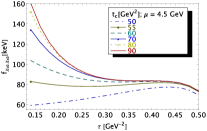
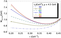
Figure 2: The coupling $f_{\chi_{c0}\chi_{c0}}$ and mass $M_{\chi_{c0}\chi_{c0}}$ at NLO as function of $\tau$ for different values of $t_{c}$, for $\mu=4.5$ GeV and for the QCD parameters in Table 2.

We consider as final results the mean of the value corresponding to the beginning of $\tau$ stability for $[t_{c}\,(\nobreak\,\mbox{GeV}),\,\tau\,(\nobreak\,\mbox{GeV}^{-2})]\simeq[55,\,0.36]$ and the one where the $t_{c}$ stability is reached for $[t_{c}\,(\nobreak\,\mbox{GeV}),\,\tau\,(\nobreak\,\mbox{GeV}^{-2})]\simeq[70,\,0.38]$.

8.2 $\mu$-stability

Using the fact that the final results must be independent of the arbitrary parameter $\mu$, we consider as optimal result the one at the inflexion point for $\mu\simeq 4.5$ GeV (Fig. 3).

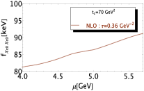
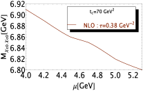
Figure 3: $\mu$-behavior of $f_{\chi_{c0}\chi_{c0}}$ and $M_{\chi_{c0}\chi_{c0}}$ for $t_{c}=70$ GeV² at NLO.

8.3 The Factorization assumption

We have shown explicitly in [3] that the contributions from the non-factorized diagrams appear at LO of perturbative series and for the $\langle\alpha_{s}G^{2}\rangle$ contributions. However, as we can see in Fig. 4, the effect of these non-factorized diagrams is relatively small (about $1/(10N_{c})$) compared to the total $F\oplus NF$ contributions. This feature justifies our approximation by using only the factorized part diagrams in the NLO perturbative contributions (see Section 5).

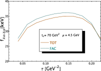
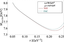
Figure 4: Comparison of the factorized (FAC) and F$\oplus$NF (TOT) at LO including $\langle\alpha_{s}G^{2}\rangle$ contribution for $t_{c}=70$ GeV² and $\mu=4.5$ GeV.

8.4 The PT series

At LO, the two definitions of the quark mass lead to different predictions while at NLO this ambiguity between the running and pole quark mass definition is avoided. From the predictions for the running mass [3] the effect of the PT corrections can be parametrized numerically as:

$$f_{\chi_{c0}\chi_{c0}} \approx 43~{}\mbox{keV}\,(1+8.7a_{s}\pm 7.57a^{2}_{s})~{},$$

$$M_{\chi_{c0}\chi_{c0}} \approx 7.76~{}\mbox{GeV}\,(1-0.5a_{s}\pm 0.25a^{2}_{s})~{},$$ (12)

where the $a^{2}_{s}$ contributions have been estimated from a geometric growth of the PT coefficients [38] and considered as an estimate of the uncalculated higher order terms of the PT series. One can notice from Eq. 12 that the PT series converge numerically but induce a relatively large systematic error for the coupling.

Table 3: $0^{++}$ fully heavy molecules/tetraquarks couplings and masses predictions from LSR at NLO. The errors from QCD input parameters are from Table 2. $|\Delta\mu|=0.20$ (resp. 0.25) GeV for the charm (resp. beauty) case. $|\Delta\tau|=0.02$ GeV^-2. In the case of asymetric errors, we take the mean value.

Observables	$\Delta t_{c}$		$\Delta\tau$		$\Delta\mu$		$\Delta m$		$\Delta\alpha_{s}$		$\Delta\alpha_{s}G^{2}$		$\Delta G^{3}-OPE$		$\Delta HO-PT$		Values
$q\equiv c,b$	c	b	c	b	c	b	c	b	c	b	c	b	c	b	c	b	c	b
$f_{{}_{\mathcal{M},\mathcal{T}}}$[ keV]
$0^{++}$ Molecule
$\overline{\chi}_{q0}\chi_{q0}$	2.80	0.01	0.40	0.10	2.50	0.10	3.70	0.50	3.50	0.70	1.20	0.10	11.5	0.60	16.0	0.20	69$\pm$21	4.0$\pm$1.1
$\overline{\eta}_{q}\eta_{q}$	0.80	0.40	0.20	0.10	3.0	0.20	10.0	1.20	5.0	2.0	0.70	0.10	12.2	0.80	0.90	0.20	56$\pm$17	9.8$\pm$2.4
$\overline{J\psi}J\psi,\,\overline{\Upsilon}\Upsilon$	4.60	0.60	1.0	0.60	2.0	0.10	10.7	4.30	19.0	2.50	3.40	0.40	45.6	3.80	0.40	0.0	160$\pm$51	23.4$\pm$6.3
$\overline{\chi}_{q1}\chi_{q1}$	0.90	1.60	1.10	0.90	0.90	0.20	6.0	3.0	9.0	4.80	10.0	0.0	4.0	3.0	5.0	19.0	162$\pm$16	48.9$\pm$20.1
$0^{++}$ Tetraquark
Table 1
$\overline{P}_{q}P_{q}$	1.40	1.80	0.40	2.30	3.40	0.50	7.20	1.0	3.50	1.0	1.30	0.10	8.90	3.50	4.80	1.20	60$\pm$14	6.5$\pm$4.9
$\overline{S}_{q}S_{q}$	0.10	0.10	0.70	0.20	9.0	2.30	20.0	2.30	9.0	3.70	0.30	0.10	7.0	9.0	87.0	0.10	249$\pm$90	29.6$\pm$10.2
$\overline{A}_{q}A_{q}$	1.40	4.10	1.0	7.20	1.50	3.40	19.2	4.0	8.80	6.40	0.40	0.0	10.0	2.80	65.0	27.0	220$\pm$69	87.4$\pm$29.5
$\overline{V}_{q}V_{q}$	5.20	0.40	1.0	0.30	6.50	0.30	11.8	1.50	5.40	2.40	1.90	0.20	9.0	0.30	0.90	0.10	102$\pm$18	17.2$\pm$2.9
Eq. 3
$\overline{A}_{q}A_{q}$	3.0	3.6	1.5	2.0	4.8	2.0	37.5	7.70	17.6	12.3	0.80	0.10	12.0	7.0	108	72.0	448$\pm$117	136$\pm$74
$M_{{}_{\mathcal{M},\mathcal{T}}}$[ MeV]
$0^{++}$ Molecule
$\overline{\chi}_{q0}\chi_{q0}$	11	39	8.0	28	10	24	47	36	19	18	29	13	76	112	9.0	8.0	6675$\pm$98	19653$\pm$131
$\overline{\eta}_{q}\eta_{q}$	23	4.0	3.0	15	23	26	51	29	24	49	14	13	186	58	3.8	1.6	6029$\pm$198	19259$\pm$88
$\overline{J\psi}J\psi,\,\overline{\Upsilon}\Upsilon$	34	31	11	42	24	27	27	52	49	30	31	22	359	116	1.3	0.0	6376$\pm$367	19430$\pm$145
$\overline{\chi}_{q1}\chi_{q1}$	26	4.0	29	99	20	22	42	25	20	43	5.0	22	16	73	7.0	6.0	6494$\pm$66	19770$\pm$137
$0^{++}$ Tetraquark
Table 1
$\overline{P}_{q}P_{q}$	34	10	19	40	23	24	46	28	20	46	30	22	258	23	22	5.0	6795$\pm$268	19754$\pm$79
$\overline{S}_{q}S_{q}$	12	1.0	28	38	21	26	54	29	43	59	1.0	2.0	25	89	9.0	9.0	6411$\pm$83	19217$\pm$120
$\overline{A}_{q}A_{q}$	26	37	32	132	20	23	43	25	21	43	2.0	1.0	38	53	0.0	10	6450$\pm$75	19872$\pm$156
$\overline{V}_{q}V_{q}$	59	27	10	22	26	4.0	47	29	25	50	21	15	152	39	1.0	0.10	6462$\pm$175	19489$\pm$79
Eq. 3
$\overline{A}_{q}A_{q}$	4.0	21	3.0	95	21	25	43	27	21	47	2.0	0.0	39	30	16	2.0	6471$\pm$67	19717$\pm$118

9 Confrontation with some LO results and data

$\bullet$ Comparison with some LO QSSR and MOM results

Using the ratio of moments in Eq. 13 we evaluate the mass of $\overline{\chi}_{q0}\chi_{q0}$ and $\overline{S}_{c}S_{c}$:

$$\mathcal{M}_{n}(Q^{2}_{0}) = \frac{1}{\pi}\int^{\infty}_{16m^{2}_{Q}}dt\frac{\mbox{Im}\Pi_{\mathcal{M,T}}(t)}{(t+Q^{2}_{0})^{n}}~{},$$

$$M^{2}_{\mathcal{M,T}} = \frac{\mathcal{M}_{n}(Q^{2}_{0})}{\mathcal{M}_{n+1}(Q^{2}_{0})}-Q^{2}_{0}~{},$$ (13)

– From MOM at NLO $\oplus\,\langle\alpha_{s}G^{2}\rangle$, we obtain:

$$M_{\chi_{c0}\chi_{c0}}\simeq 6.93\,\mbox{GeV}\,,~{}~{}M_{S_{c}S_{c}}\simeq 6.38\,\mbox{GeV},$$ (14)

compared to the ones from LSR in Table 3, these results indicate that the predictions from the two methods (LSR and MOM) are in agreement within the error.
– From MOM at LO$\,\oplus\,\langle\alpha_{s}G^{2}\rangle$:

$$M_{\chi_{c0}\chi_{c0}}\simeq 6.78\,\mbox{GeV}\,,~{}~{}M_{\chi_{b0}\chi_{b0}}\simeq 19.53\,\mbox{GeV},$$ (15)

which are lower than the ones from [39]. With the inclusion of the $\alpha_{s}$ QCD corrections, our LSR predictions for the charm and $\overline{P}_{b}P_{b}$ cases are in good agreement within the error with the LO ones from [39]. However, for the $\overline{S}_{b}S_{b},\,\overline{A}_{b}A_{b}$ and $\overline{V}_{b}V_{b}$ states our results disagree. Due to the difficulty to compare the expressions of the full correlator in [39] with the spectral function we cannot trace back the discrepancy.
– Using Eq. 3, our masses predictions from LSR at LO for $\overline{A}_{q}A_{q}$:

$$M_{A_{c}A_{c}}\simeq 6.50\,\mbox{GeV},~{}~{}M_{A_{b}A_{b}}\simeq 19.49\,\mbox{GeV},$$ (16)

are lower than the one of [40]. The estimated masses of $\overline{A}_{q}A_{q}$ from [39] are higher (resp. lower) than the ones from [40] for the charm (resp. bottom) channel. Such discrepancies may be explained by an unusual treatment of the sum rules by the author of [40].

$\bullet$ Confrontation with experiments

We conclude from the previous analysis that:
– The broad structure around (6.2$\sim$6.7) GeV might be explained by the $\overline{\eta}_{c}\eta_{c},\,\overline{\chi}_{c1}\chi_{c1}$ and $\overline{J/\psi}J/\psi$ molecules or/and the $\overline{S}_{c}S_{c},\,\overline{A}_{c}A_{c}$ and $\overline{V}_{c}V_{c}$ tetraquarks.
– The narrow structure around 6.9 GeV, if it is a $0^{++}$ state, can be identified with a $\overline{\chi}_{c0}\chi_{c0}$ molecule or $\overline{P}_{c}P_{c}$ tetraquark.
– The $\overline{\chi}_{c1}\chi_{c1}$ predicted mass is below the $\chi_{c1}\chi_{c1}$ threshold, while for the beauty state all of the predicted masses are above the $\eta_{b}\eta_{b}$ and $\Upsilon(1S)\Upsilon(1S)$ thresholds.
– Our predictions cannot clearly disentangle the mass of a molecule from a tetraquark state with the same quantum numbers.

10 Conclusions

We have presented improved predictions of QSSR for the masses and couplings of fully heavy $0^{++}$ molecules and four-quarks states at NLO of PT series and including non-perturbative $\langle\alpha_{s}G^{2}\rangle$ and $\langle G^{3}\rangle$ contributions. Using our calculation method, the effect of the heavy quark condensate is included into the gluon condensate one [41, 42, 43]. We can see a good convergence of the PT series after including higher order corrections which confirms the veracity of our results. Our analysis has been done within stability criteria with respect to the LSR variable $\tau$, the QCD continuum threshold $t_{c}$ and the subtraction constant $\mu$ which have provided successful predictions in different hadronic channels [6, 4, 7, 11, 44, 45, 46, 47, 48]. The optimal values of the masses and couplings have been extracted at the same value of these parameters where the stability appears as an extremum and/or inflection point. We have taken as a final result, the mean obtained with and without the $\langle G^{3}\rangle$ contribution and considered the error induced in this way as systematics due to the truncation of the OPE.
In a future work, we plan to evaluate the spectra and widths of $2^{++}$ four-quark states.

References

- [1] R. Aaij et al. (LHCb Collaboration), Science Bulletin 65 (2020) 1983-1993
- [2] L. An (LHCb Collaboration), LHC-CERN seminar (2020), https://indico.cern.ch/event/900972
- [3] R. M. Albuquerque et al., Phys. Rev. D 102, 094001 (2020).
- [4] J.S. Bell and R.A. Bertlmann, Nucl. Phys. B177 (1981) 218; Nucl. Phys. B187 (1981) 285.
- [5] C. Becchi et al., Z. Phys. C 8, 335 (1981).
- [6] R.A. Bertlmann, Acta Phys. Austriaca 53, 305 (1981) and references therein.
- [7] R.A. Bertlmann and H. Neufeld, Z. Phys. C 27 (1985) 437.
- [8] S. Narison and E. de Rafael, Phys. Lett. B 522 (2001) 266.
- [9] M.A. Shifman, A.I. Vainshtein and V.I. Zakharov, Nucl. Phys. B147 (1979) 385, 448.
- [10] V.I. Zakharov, Int. J. Mod. Phys. A 14, 4865 (1999).
- [11] S. Narison, QCD as a theory of hadrons, Cambridge Monogr. Part. Phys. Nucl. Phys. Cosmol. 17 (2002) 1; [hep-ph/0205006].
- [12] S. Narison, QCD spectral sum rules , World Sci. Lect. Notes Phys. 26 (1989) 1.
- [13] S. Narison, Phys. Rept. 84 (1982) 263; Acta Phys. Pol. B 26 (1995) 687.
- [14] E. de Rafael, hep-ph/9802448.
- [15] F. J. Yndurain, The Theory of Quark and Gluon Interactions, 3rd ed. (Springer, New York, 1999).
- [16] P. Pascual and R. Tarrach, QCD: Renormalization for Practitioner (Springer, New York, 1985).
- [17] L. J. Reinders, H. Rubinstein, and S. Yazaki, Phys. Rep. 127, 1(1985).
- [18] B. L. Ioffe, Prog. Part. Nucl. Phys. 56, 232(2006).
- [19] H. G. Dosch, Non-Perturbative Methods, edited by S. Narison (World Scientific, Singapor,1985).
- [20] R. Albuquerque et al., Phys. Lett. B 175, (2012) 129.
- [21] R. Albuquerque et al., Int. J. Mod. Phys. A31 (2016) no. 36, 1650196.
- [22] R. M. Albuquerque et al., Nucl. Part. Phys. Proc. 282-284, (2017) 83 ; Nucl. Part. Phys. Proc. 300-302, (2018) 186-195.
- [23] R. Albuquerque et al., Int. J. Mod. Phys. A33 (2018), 1850082.
- [24] A. Pich and E. de Rafael, Phys. Lett. B158 (1985) 477.
- [25] S. Narison and A. Pivovarov, Phys. Lett. B 327 (1994) 341.
- [26] D. J. Broadhurst, Phys. Lett. 101B, (1985) 423.
- [27] R. Albuquerque et al., Int. J. Mod. Phys. A31 (2016) no.17, 1650093.
- [28] R. Albuquerque et al., Nucl. Phys. A 1007 (2021) 122113.
- [29] R. M. Albuquerque, S. Narison and D. Rabetiarivony, arXiv:2101.07281v1 [hep-ph].
- [30] R. M. Albuquerque et al., J. Phys. G 46, 093002 (2019).
- [31] R. Tarrach, Nucl. Phys. B 183, (1981) 384.
- [32] R. Coquereaux, Ann. Phys. 125 (1980) 401 .
- [33] P. Binetruy, T. Sücker, Nucl. Phys. B 178, (1981) 293.
- [34] S. Narison, Phys. Lett. B 197 (1987) 405 ; Phys. Lett. B 216 (1989) 191.
- [35] S. Narison, Int. J. Mod. Phys. A 33 1850045 (2018); 33, 1850045(E) (2018), and references therein.
- [36] S. Narison, Phys. Lett. B 784, 261 (2018) ; Phys. Lett. B 802, 135221 (2020).
- [37] S. Narison, Phys. Lett. B 693, 559 (2010) ; 705, 544(E) (2011) ; Phys. Lett. B 706, 412 (2011) ; Phys. Lett. B 707, 259 (2012).
- [38] S. Narison and V. I. Zakharov, Phys Phys. Lett. B 679, (2009) 355.
- [39] W. Chen et al., Phys. Lett. B 773, 247 (2017).
- [40] Z. G. Wang, Eur. Phys. J. C 77, 432 (2017).
- [41] D. Broadhurst and C. Generalis, Phys. Lett. 139B, 85 (1984); Phys. Lett. 165B, 175 (1985).
- [42] E. Bagan et al., Nucl. Phys. B254, 555 (1985).
- [43] E. Bagan et al., Z. Phys. C 32, 43 (1986).
- [44] S. Narison, Phys. Lett. B 721, 269 (2013).
- [45] R.A. Bertlmann, Nucl. Phys. B 204, 387 (1982).
- [46] R.A. Bertlmann, Non-Perturbative Methods, edited by S. Narison (World Scientific Company, Singapore, 1985).
- [47] J. Marrow, J. Parker and G. Shaw, Z. Phys. C 37, 103 (1987).
- [48] S. Narison, Int. J. Mod. Phys. A 30 1550116 (2015) and references therein.