Muddling Labels for Regularization, a novel approach to generalization

Abstract

Generalization is a central problem in Machine Learning. Indeed most prediction methods require careful calibration of hyperparameters usually carried out on a hold-out validation dataset to achieve generalization. The main goal of this paper is to introduce a novel approach to achieve generalization without any data splitting, which is based on a new risk measure which directly quantifies a model’s tendency to overfit. To fully understand the intuition and advantages of this new approach, we illustrate it in the simple linear regression model ($Y=X\beta+\xi$) where we develop a new criterion. We highlight how this criterion is a good proxy for the true generalization risk. Next, we derive different procedures which tackle several structures simultaneously (correlation, sparsity,…). Noticeably, these procedures concomitantly train the model and calibrate the hyperparameters. In addition, these procedures can be implemented via classical gradient descent methods when the criterion is differentiable w.r.t. the hyperparameters. Our numerical experiments reveal that our procedures are computationally feasible and compare favorably to the popular approach (Ridge, LASSO  and Elastic-Net combined with grid-search cross-validation) in term of generalization. They also outperform the baseline on two additional tasks: estimation and support recovery of $\beta$. Moreover, our procedures do not require any expertise for the calibration of the initial parameters which remain the same for all the datasets we experimented on.

Introduction

Generalization is a central problem in machine learning. Regularized or constrained Empirical Risk Minimization (ERM) is a popular approach to achieve generalization (Kukačka et al., 2017). Ridge (Hoerl and Kennard, 1970), LASSO  (Tibshirani, 1996) and Elastic-net (Zou and Hastie, 2005) belong to this category. The regularization term or the constraint is added in order to achieve generalization and to enforce some specific structures on the constructed model (sparsity, low-rank, coefficient positiveness,…). This usually involves introducing hyperparameters which require calibration. The most common approach is data-splitting. Available data is partitioned into a training/validation-set. The validation-set is used to evaluate the generalization error of a model built using only the training-set.

Several hyperparameter tuning strategies were designed to perform hyperparameter calibration: Grid-search, Random search (Bergstra and Bengio, 2012) or more advanced hyperparameter optimization techniques (Bergstra et al., 2011; Bengio, 2000; Schmidhuber, 1987). For instance, BlackBox optimization (Brochu et al., 2010) is used when the evaluation function is not available (Lacoste et al., 2014). It includes in particular Bayesian hyperparametric optimization such as Thompson sampling (Močkus, 1975; Snoek et al., 2012; Thompson, 1933). These techniques either scale exponentially with the dimension of the hyperparameter space, or requires a smooth convex optimization space (Shahriari et al., 2015). Highly non-convex optimization problems on a high dimensionnal space can be tackled by Population based methods (Genetic Algorithms(Chen et al., 2018; Real et al., 2017; Olson et al., 2016), Particle Swarm (Lorenzo et al., 2017; Lin et al., 2008)) but at a high computational cost. Another family of advanced methods, called gradient-based techniques, take advantage of gradient optimization techniques (Domke, 2012) like our method. They fall into two categories, Gradient Iteration and Gradient approximation. Gradient Iteration directly computes the gradient w.r.t. hyperparameters on the training/evaluation graph. This means differentiating a potentially lengthy optimization process which is known to be a major bottleneck (Pedregosa, 2016). Gradient approximation is used to circumvent this difficulty, through implicit differentiation (Larsen et al., 1996; Bertrand et al., 2020). However, all these advanced methods require data-splitting to evaluate the trained model on a hold-out $validation$-set, unlike our approach.

Another approach is based on unbiased estimation of the generalization error of a model (SURE (Stein, 1981), $AIC$ (Akaike, 1974), $C_{p}$-Mallows (Mallows, 2000)) on the $training$-set. Meanwhile, other methods improve generalization during the training phase without using a hold-out $validation$-set. For instance, Stochastic Gradient Descent and the related batch learning techniques (Bottou, 1998) achieve generalization by splitting the training data into a large number of subsets and compute the Empirical Risk (ER) on a different subset at each step of the gradient descent. This strategy converges to a good estimation of the generalization risk provided a large number of observations is available. Bear in mind this method and the availability of massive datasets played a crucial role in the success of Deep neural networks. Although batch size has a positive impact on generalization (He et al., 2019), it cannot maximize generalization on its own.

Model aggregation is another popular approach to achieve generalization. It concerns for instance Random Forest (Ho, 1995; Breiman, 2001), MARS (Friedman, 1991) and Boosting (Freund and Schapire, 1995). This approach aggregates weak learners previously built using bootstrapped subsets of the $training$-set. The training time of these models is considerably lengthened when a large number of weak learners is considered, which is a requirement for improved generalization. Recall XGBOOST (Chen and Guestrin, 2016) combines a version of batch learning and model aggregation to train weak learners.
MARS, Random Forest, XGBOOST and Deep learning have obtained excellent results in Kaggle competitions and other machine learning benchmarks (Fernández-Delgado et al., 2014; Escalera and Herbrich, 2018). However these methods still require regularization and/or constraints in order to generalize. This implies the introduction of numerous hyperparameters which require calibration on a hold-out $validation$-set for instance via Grid-search. Tuning these hyperparameters requires expensive human expertise and/or computational resources.

We approach generalization from a different point of view. The underlying intuition is the following. We no longer see generalization as the ability of a model to perform well on unseen data, but rather as the ability to avoid finding pattern where none exist. Using this approach, we derive a novel criterion and several procedures which do not require data splitting to achieve generalization.

This paper is intended to be an introduction to this novel approach. Therefore, for the sake of clarity, we consider here the linear regression setting but our approach can be extended to more general settings like deep learning.

Let us consider the linear regression model:

$$\mathbf{Y}=\mathbb{X}\beta^{*}+\bm{\xi},$$ (1)

where $\mathbb{X}^{\top}=(\mathbf{X}_{1},\cdots,\mathbf{X}_{n})$ is the $n\times p$ design matrix and the $n$-dimensional vectors $\mathbf{Y}=(Y_{i},\cdots,Y_{n})^{\top}$ and $\bm{\xi}=(\xi_{1},\cdots,\xi_{n})^{\top}$ are respectively the response and the noise variables. Throughout this paper, the noise level $\sigma>0$ is unknown. Set $||\mathbf{v}||_{n}=(\frac{1}{n}\sum_{i=1}^{n}v_{i}^{2})^{1/2}$ for any $\mathbf{v}=(v_{1},\ldots,v_{n})^{\top}\in\mathbb{R}^{n}$.

In practice, the correlation between $\mathbf{X}_{i}$ and $Y_{i}$ is unknown and may actually be very weak. In this case, $\mathbf{X}_{i}$ provides very little information about $Y_{i}$ and we expect from a good procedure to avoid building a spurious connection between $\mathbf{X}_{i}$ and $Y_{i}$. Therefore, by understanding generalization as do not fit the data in non-informative cases, we suggest creating an artificial dataset which preserves the marginal distributions while the link between $\mathbf{X}_{i}$ and $Y_{i}$ has been completely removed. A simple way to do so is to construct an artificial set $\widetilde{\mathcal{D}}=({\mathbb{X}},\widetilde{\mathbf{Y}})=(\mathbb{X},\pi(\mathbf{Y}))$ by applying permutations $\pi\in\mathfrak{S}_{n}$ (the set of permutations of $n$ points) on the components of $\mathbf{Y}$ of the initial dataset $\mathcal{D}$ where for any $\mathbf{y}\in\mathbb{R}^{n}$, we set $\pi(\mathbf{y})=(y_{\pi(1)},\ldots,y_{\pi(n)})^{\top}$.

The rest of the paper is organized as follows. In Section 1 we introduce our novel criterion and highlight its generalization performance. In Section 2, this new approach is applied to several specific data structures in order to design adapted procedures which are compatible with gradient-based optimization methods. We also point out several advantageous points about this new framework in an extensive numerical study. Finally we discuss possible directions for future work in Section 3.

1 Label muddling criterion

In model (1), we want to recover $\beta^{*}$ from $\mathcal{D}=(\mathbb{X},\mathbf{Y})$. Most often, the $n$ observations are partitioned into two parts of respective sizes $n_{train}$ and $n_{val}$, which we denote the $train$-set $(\mathbb{X}_{train},\mathbf{Y}_{train})$ and the $validation$-set $(\mathbb{X}_{val},\mathbf{Y}_{val})$ respectively. The $train$-set is used to build a family of estimators $\{\beta(\theta,\mathbb{X}_{train},\mathbf{Y}_{train})\}_{\theta}$ which depends on a hyperparameter $\theta$. Next, in order to achieve generalization, we use the $validation$-set to calibrate $\theta$. This is carried out by minimizing the following empirical criterion w.r.t. $\theta$:

$$\|\mathbf{Y}_{val}-\mathbb{X}_{val}\,\beta(\theta,\mathbb{X}_{train},\mathbf{Y}_{train})\|_{n_{val}}.$$

In our approach, we use the complete dataset $\mathcal{D}$ to build the family of estimators and to calibrate the hyperparameter $\theta$.

Definition 1.

Fix $T\in\mathbb{N}^{*}$. Let $\{\pi^{t}\}_{t=1}^{T}$ be $T$ permutations in $\mathfrak{S}_{n}$. Let $\{\beta(\theta,\cdot,\cdot)\}_{\theta}$ be a family of estimator.

The MLR  criterion is defined as:

$$\textit{{MLR}}_{\beta}(\theta)=\|\mathbf{Y}-\mathbb{X}\beta(\theta,\mathbb{X},\mathbf{Y})\|_{n}$$

$$\hskip 56.9055pt-\frac{1}{T}\sum_{t=1}^{T}\|\pi^{t}(\mathbf{Y})-\mathbb{X}\beta(\theta,\mathbb{X},\pi^{t}(\mathbf{Y}))\|_{n}.$$ (2)

The MLR  criterion performs a trade-off between two antagonistic terms. The first term fits the data while the second term prevents overfitting. Since the MLR  criterion is evaluated directly on the whole sample without any hold-out $validation$-set, this approach is particularly useful for small sample sizes where data-splitting approaches can produce strongly biased performance estimates (Vabalas et al., 2019; Varoquaux, 2018).
We highlight in the following numerical experiment the remarkable generalization performance of the MLR  criterion.

NUMERICAL EXPERIMENTS.

We consider two families

$$\mathcal{F}(\theta)=\{\beta(\theta,\mathbb{X}_{train},\mathbf{Y}_{train})\}_{\theta}$$

of estimators constructed on a $train$-dataset and indexed by $\theta$: Ridge and LASSO  . We are interested in the problem of calibration of the hyperparameter $\theta$ on a grid $\Theta$. We compare two criteria $\mathcal{C}(\theta)$ to calibrate $\theta$: the MLR  criterion and cross-validation (implemented as Ridge, Lasso in Scikit-learn (Pedregosa et al., 2011)). For each criterion $\mathcal{C}(\theta)$, the final estimator $\widehat{\beta}_{train}=\beta(\widehat{\theta},\mathbb{X}_{train},\mathbf{Y}_{train})$ is $s.t.$

$$\widehat{\theta}=\underset{\theta\in\Theta}{\arg\min}\,\mathcal{C}(\theta).$$

$\mathbf{R^{2}}$-score.

For each family, the generalization performance of each criterion is evaluated using the hold-out $test$-dataset $\mathcal{D}_{test}=(\mathbb{X}_{test},\mathbf{Y}_{test})$ by computing the following $\mathbf{R^{2}}$-scores:

$$\mathbf{R^{2}}(\widehat{\beta}_{train})=1-\frac{\|\mathbf{Y}_{test}-\mathbb{X}_{test}\,\widehat{\beta}_{train}\|_{2}}{\|\mathbf{Y}_{test}-\overline{\mathbf{Y}}_{test}\mathbbm{1}_{n}\|_{2}}\,(\leq 1),$$ (3)

where $\overline{\mathbf{Y}}_{test}$ is the empirical mean of $\mathbf{Y}_{test}$. For the sake of simplicity, we set $\mathbf{R^{2}}(\widehat{\theta})=\mathbf{R^{2}}(\widehat{\beta}_{train})$. The oracle we aim to match, is

$$\theta^{*}=\underset{\theta\in\Theta}{\arg\min}\,\mathbf{R^{2}}(\theta).$$

Our first numerical experiments concern synthetic data.

Synthetic data.

For $p=80$, we generate observations $(\mathbf{X},Y)\in\mathbb{R}^{p}\times\mathbb{R}$, $s.t.$ $Y=\mathbf{X}^{\top}\beta^{*}+\epsilon$, with $\epsilon\sim\mathcal{N}(0,\sigma)$, $\sigma=10$ or $50$. We consider three different scenarii. Scenario A (correlated features) corresponds to the case where the LASSO  is prone to fail and Ridge should perform better. Scenario B (sparse setting) corresponds to a case known as favorable to LASSO  . Scenario C combines sparsity and correlated features. For each scenario we sample a $train$-dataset of size $n_{train}=100$ and a $test$-dataset of size $n_{test}=1000$.
For each scenario, we perform $M=100$ repetitions of the data generation process to produce $M$ pairs of $train$/$test$ datasets. Details on the data generation process can be found in the Appendix.

Performances evaluation.

For each family $\mathcal{F}(\theta)$ and each criterion $\mathcal{C}(\theta)$, we construct on every $train$-dataset, the corresponding model $\widehat{\beta}_{train}$. Next, using the corresponding hold-out $test$-dataset $\mathcal{D}_{test}=(\mathbb{X}_{test},\mathbf{Y}_{test})$, we compute their $\mathbf{R^{2}}$-scores.

Impact of $\,T$.

In Figure 1 we study the impact of the number of permutations $T$ on the generalization performance of the criterion measured via the $R^{2}$-score in (3). The most striking finding is the sharp increase in the generalization performance from the first added permutation in Scenarios A and C. Adding more permutations does not impact the generalization but actually improves the running time and stability of the novel procedures which we will introduce in the next section. In a pure sparsity setting (Scenario B with LASSO), adding permutations marginally increases the generalization.

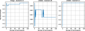
Figure 1: Variation of the $R^{2}$-score w.r.t. the number of permutation.

Comparison of generalization performance.

For Scenario A with the Ridge family, we compute the difference $\mathbf{R^{2}}(\widehat{\theta}^{\mathcal{C}(\theta)})-\mathbf{R^{2}}(\theta^{*}),$ for the two criteria $\mathcal{C}(\theta)$ (MLR  and CV). For Scenarios B and C, we consider the LASSO  family and compute the same difference. Boxplots in Figure 2 summarize our finding over 100 repetitions of the synthetic data. The empirical mean is depicted by a green triangle on each boxplot. Moreover, to check for statistically significant margin in $\mathbf{R^{2}}$-scores between different procedures, we use the Mann-Whitney test (as detailed in (Kruskal, 1957) and implemented in scipy (Virtanen et al., 2020)). The boxplots highlighted in yellow correspond to the best procedures according to the Mann-Whitney (MW) test.

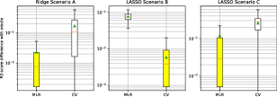
Figure 2: Generalization performance for MLRand CV for Ridge and LASSO  Hyperparameter calibration

As we observed, the MLR  criterion performs better than CV for the calibration of the Ridge and LASSO hyperparameters in Scenarios A and C in the presence of correlation in the design matrix.

Plot of the generalization performance.

In order to plot the different criteria together, we use the following rescaling. Let $F\,:\,\Theta\rightarrow\mathbb{R}$, we set

$$\underline{\theta}=\underset{\theta\in\Theta}{\arg\min}\,F(\theta)\,\text{ and }\,\overline{\theta}=\underset{\theta\in\Theta}{\arg\max}\,F(\theta).$$

For any $\theta\in\Theta$, we define

$$\Lambda_{F}(\theta)=\frac{F(\theta)-F(\underline{\theta})}{F(\overline{\theta})-F(\underline{\theta})}.$$

Figure 3 contains the rescaled versions of the $\mathbf{R}^{2}$-score on the test set and the MLR and $CV$ criteria computed on the $train$-dataset. The vertical lines correspond to the selected values of the hyperparameter in the grid $\Theta$ by the MLR  and CV criteria as well as the optimal hyperparameter $\theta^{*}$ for the $\mathbf{R}^{2}$-score on the test set. The MLR  criterion is a good proxy for the generalization performance ($R^{2}$- score on the $test$-dataset) on the whole grid $\Theta$ for the Ridge in Scenario A. In Scenario C with the LASSO, the MLR  criterion is a smooth function with steep variations in a neighborhood of its global optimum. This is an ideal configuration for the implementation of gradient descent schemes.

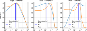
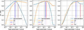
Figure 3: Criterion landscape for grid-search calibration with MLR  (Up) and CV (down).

the MLR criterion performs better than CV on correlated data for grid-search calibration of the LASSO and Ridge hyperparameters. However CV works better in the pure sparsity scenario. This motivated the introduction of novel procedures based on the MLR  principle which can handle the sparse setting better.

2 Novel procedures

In Section 1, we used (1) to perform grid-search calibration of the hyperparameter. However, if $\{\beta(\theta)\}_{\theta}$ is a family of models differentiable w.r.t. $\theta$, we can minimize (1) w.r.t. $\theta$ via standard gradient-based methods. This motivated the introduction of new procedures based on the MLR  criterion.

Definition 2.

Consider $\{\beta(\theta)\}_{\theta}$ a family of models differentiable w.r.t. $\theta$. Let $\{\pi^{t}\}_{t=1}^{T}$ be $T$ derangements in $\mathfrak{S}_{n}$. The $\beta$-MLR  procedure is

$$\begin{array}[]{lcl}\widehat{\beta}=\beta(\widehat{\theta})&\text{with}&\widehat{\theta}=\underset{\theta}{\arg\min}\,\textit{{MLR}}_{\beta}(\theta).\end{array}$$ (5)

where $\textit{{MLR}}_{\beta}$ is defined in (1).

Moreover, using our approach, we can also enforce several additional structures simultaneously (sparsity, correlation, group sparsity, low-rank,…) by constructing appropriate families of models. In this regard, let us consider the 3 following procedures which do not require a hold-out $validation$-set.

R-MLR  procedure for correlated designs.

The Ridge family of estimators $\{\beta^{R}(\lambda,\mathbb{X},\mathbf{Y})\}_{\lambda>0}$ is defined as follows:

$$\beta^{R}(\lambda,\mathbb{X},\mathbf{Y})=(\mathbb{X}^{\top}\mathbb{X}+\lambda\mathbb{I}_{p})^{-1}\mathbb{X}^{\top}\mathbf{Y},\quad\lambda>0.$$ (6)

Applying Definition 2 with the Ridge family, we obtain the R-MLR  procedure $\widehat{\beta}^{\mathcal{R}}=\beta^{R}(\widehat{\lambda})$ where $\widehat{\lambda}=\underset{\lambda>0}{\arg\min}\,\textit{{MLR}}_{\beta^{R}}(\lambda)$. This new optimisation problem can be solved by gradient descent, contrarily to the previous section where we performed a grid-search calibration of $\lambda$.

S-MLR  for sparse models.

We design in Definition 3 below a novel differentiable family of models to enforce sparsity in the trained model. Applying Definition 2 to this family, we can derive the S-MLR  procedure: $\widehat{\beta}^{\mathcal{S}}=\beta^{\mathcal{S}}(\widehat{\theta})$ where $\widehat{\theta}=\underset{\theta}{\arg\min}\,\,\textit{{MLR}}_{\beta^{\mathcal{S}}}(\theta)$.

Definition 3.

Let $\{\beta^{\mathcal{S}}(\lambda,\kappa,\gamma,\mathbb{X},\mathbf{Y})\}_{(\lambda,\kappa,\gamma)\in\mathbb{R}^{*}_{+}\times\mathbb{R}^{*}_{+}\times\mathbb{R}^{p}}\,\,$ be a family closed-form estimators defined as follows:

$$\beta^{\mathcal{S}}(\lambda,\kappa,\gamma,\mathbb{X},\mathbf{Y})=\mathcal{S}(\kappa,\gamma)\beta^{R}(\lambda,\mathbb{X}\mathcal{S}(\kappa,\gamma),\mathbf{Y}),$$ (7)

where $\beta^{R}$ is defined in (6), the quasi-sparsifying function $\mathcal{S}:\mathbb{R}^{*}_{+}\times\mathbb{R}^{p}\rightarrow]0,1[^{p\times p}$ is $s.t.$

$$\mathcal{S}(\kappa,\gamma)=\text{diag}\left(\mathcal{S}_{1}(\kappa,\gamma),\cdots,\mathcal{S}_{p}(\kappa,\gamma)\right),$$

where for any $j=1,\cdots,p$,

$$\begin{array}[]{lll}\mathcal{S}_{j}\ :&\mathbb{R}^{*}_{+}\times\mathbb{R}^{p}\rightarrow]0,1[\\ &(\kappa,\gamma)\mapsto\mathcal{S}_{j}(\kappa,\gamma)=\left(1+e^{-\kappa\times(\sigma_{\gamma}^{2}+10^{-2})(\gamma_{j}-\overline{\gamma})}\right)^{-1},\end{array}$$

with $\overline{\gamma}=\frac{1}{p}\sum_{i=1}^{p}\gamma_{i}$ and $\sigma_{\gamma}^{2}=\sum_{i=1}^{p}(\gamma_{i}-\overline{\gamma})^{2}$.

The new family (7) enforces sparsity on the regression vector but also directly onto the design matrix. Hence it can be seen as a combination of data-preprocessing (performing feature selection) and model training (using the ridge estimator).
Noticeably, the quasi-sparsifying trick transforms feature selection (a discrete optimization problem) into a continuous optimization problem which is solvable via classical gradient-based methods. The function $\mathcal{S}$ produces diagonal matrices with diagonal coefficients in $]0,1[$. Although the sigmoid function $\mathcal{S}_{j}$ cannot take values 0 or 1, for very small or large values of $\gamma_{j}$, the value of the corresponding diagonal coefficient of $S(\kappa,\gamma)$ is extremely close to $0$ or $1$. In those cases, the resulting model is weakly sparse in our numerical experiments. Thresholding can then be used to perform feature selection.

A-MLR  for correlated designs and sparsity.

Aggregation is a statistical technique which combines several estimators in order to attain higher generalization performance (Tsybakov, 2003). We propose in Definition 4 a new aggregation procedure to combine the estimators (6) and (7). This essentially consists in an interpolation between $\beta^{R}$ and $\beta^{\mathcal{S}}$ models, where the coefficient of interpolation is quantified via the introduction of a new regularization parameter $\mu\in\mathbb{R}$.

Definition 4.

We consider the family of models

$$\{\beta^{\mathcal{A}}(\lambda,\kappa,\gamma,\mu,\mathbb{X},\mathbf{Y})\}_{(\lambda,\kappa,\gamma,\mu)\in\mathbb{R}^{*}_{+}\times\mathbb{R}^{*}_{+}\times\mathbb{R}^{p}\times\mathbb{R}}\,\,$$

with

$$\beta^{\mathcal{A}}(\theta,\mathbb{X},\mathbf{Y}) =\textbf{S}(\mu)\times\beta^{R}(\lambda,\mathbb{X},\mathbf{Y})$$

$$\hskip 28.45274pt+(1-\textbf{S}(\mu))\times\beta^{\mathcal{S}}(\lambda,\kappa,\gamma,\mathbb{X},\mathbf{Y}),$$ (8)

where $\beta^{R}(\lambda,\mathbf{Y})$ and $\beta^{\mathcal{S}}(\lambda,\kappa,\gamma,\mathbb{X},\mathbf{Y})$ are defined in (6) and (7) respectively and S is the sigmoid.

Applying Definition 2 to this family, we can derive the A-MLR  procedure: $\widehat{\beta}^{\mathcal{A}}=\beta^{\mathcal{A}}(\widehat{\theta})$ where $\widehat{\theta}=\underset{\theta}{\arg\min}\,\,\textit{{MLR}}_{\beta^{\mathcal{A}}}(\theta)$.

This procedure is designed to handle both correlation and sparsity.

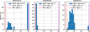
Figure 4: Distribution of the value of $\textbf{S}(\widehat{\mu})$ over $100$ repetitions on synthetic data.

Figure 4 shows $\widehat{\beta}^{\mathcal{A}}$ behaves almost as a selector which picks the most appropriate family of models between $\beta^{R}$ and $\beta^{\mathcal{S}}$. Indeed, in all scenarios, $\textbf{S}(\widehat{\mu})$ only takes values close either to $0$ or $1$ in order to adapt to the structure of the model. Moreover in Scenario B (sparsity), $\widehat{\beta}^{\mathcal{A}}$ always selects the sparse model. Indeed we always have $\textbf{S}(\widehat{\mu})\leq 0.002$ over $100$ repetitions.

Algorithmic complexity.

Using the MLR  criterion, we develop fully automatic procedures to tune regularization parameters while simultaneously training the model in a single run of the gradient descent algorithm without a hold-out $validation$ set. The computational complexity of our methods is $O(n(p+r)K)$ where $n,p,r,K$ denote respectively the number of observations, features, regularization parameters and iterations of the gradient descent algorithm. The computational complexity of our method grows only arithmetically w.r.t. the number of regularization parameters.

NUMERICAL EXPERIMENTS.

We performed numerical experiments on the synthetic data from Section 1 and also on real datasets described below.

Real data.

We test our methods on several commonly used real datasets (UCI (Asuncion and Newman, 2007) and Svmlib (Chang and Lin, 2011) repositories). See Appendix for more details. Each selected UCI dataset is splitted randomly into a $80\%$ $train$-dataset and a $20\%$ $test$-dataset. We repeat this operation $M=100$ times to produce $M$ pairs of $(train,test)$-datasets.
In order to test our procedures in the setting $n\leq p$, we selected, from Svmlib, the news20 dataset which contains a $train$ and a $test$ dataset. We fixed the number of features $p$ and we sample six new 20news $train$-datasets of different sizes $n$ from the initial news20 $train$-dataset. For each size $n$ of dataset, we perform $M=100$ repetitions of the sampling process to produce $M$ $train$-datasets. We kept the initial $test$-set for the evaluation of the generalization performances.

Number of iterations.

We choose to solve (5) using ADAM but other GD methods could be used. Figure 5 contains the boxplots of the number of ADAM iterations for the MLR  procedures on the synthetic and real datasets over the $M=100$ repetitions. Although $\textit{{MLR}}_{\beta^{\mathcal{S}}}$ and $\textit{{MLR}}_{\beta^{\mathcal{A}}}$ are highly non-convex, the number of iterations required for convergence is always about a few several dozen in our experiments. This was already observed in other non-convex settings (Kingma and Ba, 2014).

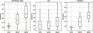
Figure 5: Synthetic, UCI and 20news data: Number of iterations

Running time.

Our procedures were coded in Pytorch to underline how they can be parallelized on a GPU. A comparison of the running time with the benchmark procedures is not pertinent as they are implemented on cpu by Scikit-learn. The main point of our experiments was rather to show how the MLR  procedures can be successfully parallelized. This opens promising prospects for the MLR  approach in deep learning frameworks.

From a computational point of view, the matrix inversion in (6) is not expensive in our setting as long as the covariance matrix can fully fit on the GPU. Figures 7 and 7 confirm the running time is linear in $n,p$ for the MLR  procedures. This confirms the MLR  procedures are scalable.

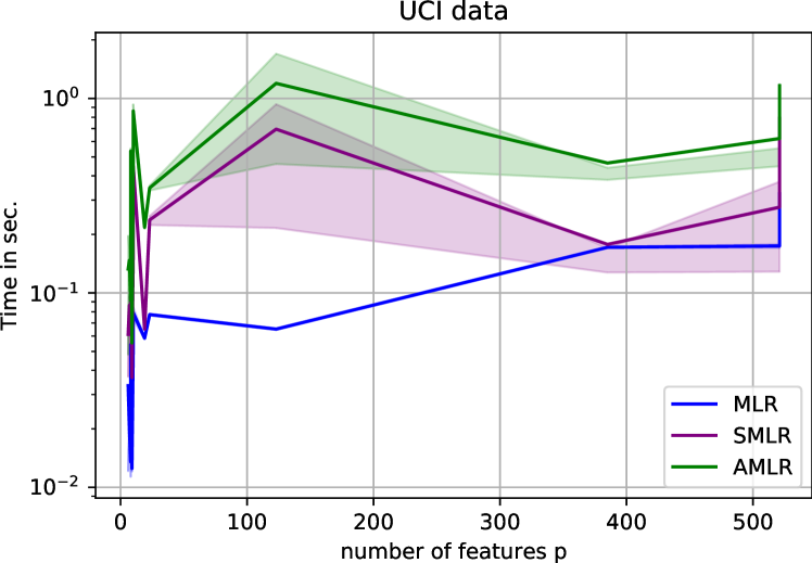
Figure 6: UCI data: running time as a function of $n$

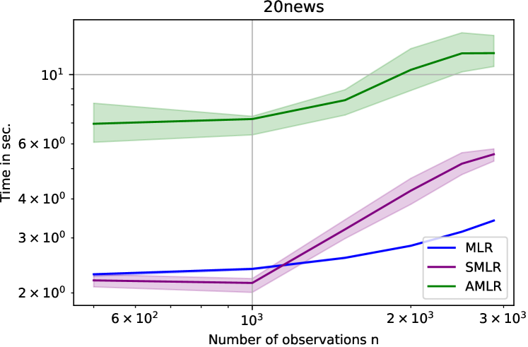
Figure 7: 20news data: running times as a function of $p$

Consequently, our procedures run in reasonable time as illustrated in Figures 8 and 9.

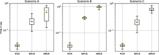
Figure 8: Synthetic data: running times in seconds.

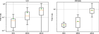
Figure 9: UCI data (left) and 20news data (right): running times .

Initial parameters.

Strinkingly, the initial values of the parameters (see Table 1) used to implement our MLR  procedures could remain the same for all the datasets we considered while still yielding consistently good prediction performances. These initial values were calibrated only once in the standard setting ($n\geq p$) on the Boston dataset (Harrison Jr and Rubinfeld, 1978; Belsley et al., 2005) which we did not include in our benchmark when we evaluated the performance of our procedures. We emphasize again we used these values without any modification on all the synthetic and real datasets. The synthetic and UCI datasets fall into the standard setting. Meanwhile, the 20news datasets correspond to the high-dimensional setting ($p\gg n$). As such, it might be possible to improve the generalization performance by using a different set of initial parameters better adapted to the high-dimensional setting. This will be investigated in future work.

However, in this paper, we did not intend to improve the generalization performance by trying to tune the initial parameters for each specific dataset. This was not the point of this project. We rather wanted to highlight our gradient-based methods compare favorably in terms of generalization with benchmark procedures just by using the default initial values in Table 1.

Optimization parameters	Parameter initialization
Tolerance $10^{-4}$ Max. iter. $10^{3}$ Learning rate $0.5$ Adam $\beta_{1}$ $0.5$ Adam $\beta_{2}$ $0.9$	$T$ $30$ $\lambda$ $10^{3}$ $\gamma$ $0_{p}$ $\kappa$ $0.1$ $\mu$ $0$

Table 1: Parameters for the MLR  procedures.

We also studied the impact of parameter $T$ on the performances of the MLR  procedures on the synthetic data. In Figure 10, the generalization performance ($\mathbf{R^{2}}$-score) increases significantly from the first added permutation ($T=1$) . Starting from $T\approx 10$, the $\mathbf{R^{2}}$-score has converged to its maximum value. An even more striking phenomenon is the gain observed in the running time when we add $T$ permutations (for $T$ in the range from $1$ to approximately $100$) when compared with the usual empirical risk ($T=0$). Larger values of $T$ are neither judicious nor needed in this approach. In addition, the needed number of iterations for ADAM to converge is divided by $3$ starting from the first added permutation. Furthermore, this number of iterations remained stable (below 20) starting from $T=1$. Based on these observations, the hyperparameter T does not require calibration. We fixed $T=30$ in our experiments even though $T=10$ might have been sufficient.

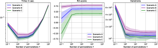
Figure 10: Synthetic data: impact of $T$ on the MLR  procedures.

Performance comparisons.

We compare our MLR  procedures against cross-validated Ridge, LASSO  and Elastic-net (implemented as RidgeCV, LassoCV and ElasticnetCV in Scikit-learn (Pedregosa et al., 2011)) on simulated and real datasets. Our procedures are implemented in PyTorch (Paszke et al., 2019) on the centered and rescaled response $\mathbf{Y}$. Complete details and results can be found in the Appendix. In our approach $\theta$ can always be tuned directly on the $train$ set whereas for benchmark procedures like LASSO  , Ridge, Elastic net, $\theta$ is typically calibrated on a hold-out $validation$-set using grid-search CV for instance.

Generalisation performance.

Figures 11 and 12 show the MLR  procedures consistently attain the highest $\mathbf{R^{2}}$-scores for the synthetic and UCI data according to the Mann-Whitney test over the $M=100$ repetitions. Regarding, the 20news datasets, the MLR  procedures are always within $0.05$ of the best (E-net).

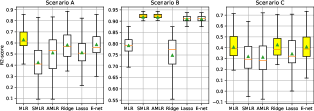
Figure 11: Synthetic data: R2-score

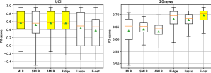
Figure 12: UCI data (left) and 20news data (right): R2-score

Estimation of $\beta^{*}$ and support recovery accuracy.

For the synthetic data, we also consider the estimation of the regression vector $\beta^{*}$. We use the $l_{2}$-norm estimation error $\|\widehat{\beta}-\beta^{*}\|_{2}$ to compare the procedures. As we can see in Figure 13, the MLR  procedures perform better than the benchmark procedures.

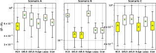
Figure 13: $\beta^{*}$ estimation (best in yellow according to MW)

We finally study the support recovery accuracy in the sparse setting (Scenario B). We want to recover the support $J(\beta^{*})=\left\{j\,:\,\beta^{*}_{j}\neq 0\right\}$. For our procedures, we build the following estimator $\widehat{J}(\widehat{\beta})=\left\{j\,:\,|\widehat{\beta}_{j}|>\widehat{\tau}\right\}$ where the threshold $\widehat{\tau}$ corresponds to the first sharp decline of the coefficients $|\widehat{\beta}_{j}|$. Denote by $\#J$ the cardinality of set $J$. The support recovery accuracy is measured as follows:

$$Acc(\widehat{\beta}):=\frac{\#\{J(\beta^{*})\cap\widehat{J}(\widehat{\beta})\}+\#\{J^{c}(\beta^{*})\cap\widehat{J}^{c}(\widehat{\beta})\#\}}{p},$$

Our simulations confirm $\widehat{\beta}^{\mathcal{S}}$ is a quasi-sparse vector. Indeed we observe in Figure 14 a sharp decline of the coefficients $|\widehat{\beta}^{\mathcal{S}}_{j}|$. Thus we set the threshold $\widehat{\tau}$ at $10^{-3}$.

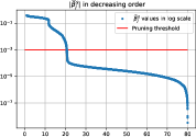
Figure 14: Coefficients values (blue) and threshold (red) with $p=80$.

Overall, $\widehat{\beta}^{\mathcal{S}}$ and $\widehat{\beta}^{\mathcal{A}}$ perform better for support recovery than the benchmark procedures. Moreover in Scenario B favorable to LASSO, our procedures perform far better (Figure 15).

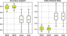
Figure 15: Support recovery performance analysis in Scenario B (best in yellow according to MW).

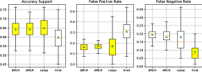
Figure 16: Support recovery performance analysis in Scenario C (best in yellow according to MW).

3 Conclusion and future work

In this paper, we introduced in the linear regression setting the new MLR  approach based on a different understanding of generalization. Exploiting this idea, we derived a novel criterion and new procedures which can be implemented directly on the $train$-set without any hold-out $validation$-set. Within MLR, additional structures can be taken into account without any significant increase in the computational complexity.

We highlighted several additional advantageous properties of the MLR  approach in our numerical experiments. The MLR  approach is computationally feasible while yielding statistical performances equivalent or better than the cross-validated benchmarks. We provided numerical evidence of MLR  criterion’s ability to generalize from the first added permutation. Besides, the strength of our MLR  procedures stems from their compatibility with gradient-based optimization methods. As such, these procedures can fully benefit from automatic graph-differentiation libraries (such as pytorch (Paszke et al., 2017) and tensorflow (Abadi et al., 2015)).

In our numerical experiments, adding more permutations improves the convergence of the ADAM optimizer while preserving generalisation. As a matter of fact, $T$ does not require any fine-tuning. In that regard, $T$ is not a hyperparameter. Likewise, the other hyperparameters require no tedious initialization in this framework. The same fixed hyperparameters for ADAM and initialization values of the regularization parameters (see Table 1) were used for all the considered datasets. Noticeably, these experiments were run using high values for learning rate and convergence threshold. Consequently, only a very small number of iterations were needed, even for non-convex criteria ($\textit{{MLR}}_{\beta^{\mathcal{S}}}$ and $\textit{{MLR}}_{\beta^{\mathcal{A}}}$).

The MLR  approach offers promising perspectives to address an impediment to the broader use of deep learning. Currently, fine-tuning DNN numerous hyper-parameters often involves heavy computational resources and manual supervision from field experts(Smith, 2018). Nonetheless, it is widely accepted that deep neural networks produce state-of-the-art results on most machine learning benchmarks based on large and structured datasets (Escalera and Herbrich, 2018; He et al., 2016; Klambauer et al., 2017; Krizhevsky et al., 2012; Silver et al., 2016; Simonyan and Zisserman, 2014; Szegedy et al., 2015). By contrast, it is not yet the case for small unstructured datasets, (eg. tabular datasets with less than 1000 observations ) where Random Forest, XGBOOST, MARS, $etc$ are usually acknowledged as the state of the art (Shavitt and Segal, 2018).

These concerns are all the more relevant during the ongoing global health crisis. Reacting early and appropriately to new streams of information became a daily challenge. Specifically, relying on the minimum amount of data to produce informed decisions on a massive scale has become the crux of the matter. In this unprecedented situation, transfer learning and domain knowledge might not be relied on to address these concerns. In that regard, the minimal need for calibration and the reliable convergence behavior of the MLR  approach are a key milestone in the search for fast reliable regularization methods of deep neural networks, especially in the small sample regime.

Beyond the results provided in this paper, we successfully extended the MLR  approach to deep neural networks. Neural networks trained with the MLR criterion can reach state of the art results on benchmarks usually dominated by Random Forest and Gradient Boosting techniques. Moreover, these results were obtained while preserving the fast, smooth and reliable convergence behavior displayed in this paper. We also successfully extended our approach to classification on tabular data. All these results are the topics of a future paper which will be posted on Arxiv soon. In an ongoing project, we are also adapting our approach to tackle few-shots learning and adversarial resilience for structured data (images, texts, graphs). We believe we just touched upon the many potential applications of the MLR  approach in the fields of Machine Learning, Statistics and Econometrics.

References

- Abadi et al. [2015] Martin Abadi, Ashish Agarwal, Paul Barham, Eugene Brevdo, Zhifeng Chen, Craig Citro, Greg S. Corrado, Andy Davis, Jeffrey Dean, Matthieu Devin, Sanjay Ghemawat, Ian Goodfellow, Andrew Harp, Geoffrey Irving, Michael Isard, Yangqing Jia, Rafal Jozefowicz, Lukasz Kaiser, Manjunath Kudlur, Josh Levenberg, Dandelion Mane, Rajat Monga, Sherry Moore, Derek Murray, Chris Olah, Mike Schuster, Jonathon Shlens, Benoit Steiner, Ilya Sutskever, Kunal Talwar, Paul Tucker, Vincent Vanhoucke, Vijay Vasudevan, Fernanda Viegas, Oriol Vinyals, Pete Warden, Martin Wattenberg, Martin Wicke, Yuan Yu, and Xiaoqiang Zheng. TensorFlow: Large-scale machine learning on heterogeneous systems, 2015. URL https://www.tensorflow.org/. Software available from tensorflow.org.
- Akaike [1974] Hirotugu Akaike. A new look at the statistical model identification. IEEE transactions on automatic control, 19(6):716–723, 1974.
- Asuncion and Newman [2007] Arthur Asuncion and David Newman. Uci machine learning repository, 2007.
- Belsley et al. [2005] David A Belsley, Edwin Kuh, and Roy E Welsch. Regression diagnostics: Identifying influential data and sources of collinearity, volume 571. John Wiley & Sons, 2005.
- Bengio [2000] Yoshua Bengio. Gradient-based optimization of hyperparameters. Neural computation, 12(8):1889–1900, 2000.
- Bergstra and Bengio [2012] James Bergstra and Yoshua Bengio. Random search for hyper-parameter optimization. Journal of machine learning research, 13(Feb):281–305, 2012.
- Bergstra et al. [2011] James S Bergstra, Rémi Bardenet, Yoshua Bengio, and Balázs Kégl. Algorithms for hyper-parameter optimization. In Advances in neural information processing systems, pages 2546–2554, 2011.
- Bertrand et al. [2020] Quentin Bertrand, Quentin Klopfenstein, Mathieu Blondel, Samuel Vaiter, Alexandre Gramfort, and Joseph Salmon. Implicit differentiation of lasso-type models for hyperparameter optimization. arXiv preprint arXiv:2002.08943, 2020.
- Bottou [1998] Léon Bottou. Online learning and stochastic approximations. On-line learning in neural networks, 17(9):142, 1998.
- Breiman [2001] Leo Breiman. Random forests. Machine learning, 45(1):5–32, 2001.
- Brochu et al. [2010] Eric Brochu, Vlad M Cora, and Nando De Freitas. A tutorial on bayesian optimization of expensive cost functions, with application to active user modeling and hierarchical reinforcement learning. arXiv preprint arXiv:1012.2599, 2010.
- Chang and Lin [2011] Chih-Chung Chang and Chih-Jen Lin. Libsvm: A library for support vector machines. ACM transactions on intelligent systems and technology (TIST), 2(3):1–27, 2011.
- Chen et al. [2018] Boyuan Chen, Harvey Wu, Warren Mo, Ishanu Chattopadhyay, and Hod Lipson. Autostacker: A compositional evolutionary learning system. In Proceedings of the Genetic and Evolutionary Computation Conference, pages 402–409, 2018.
- Chen and Guestrin [2016] Tianqi Chen and Carlos Guestrin. Xgboost: A scalable tree boosting system. In Proceedings of the 22nd acm sigkdd international conference on knowledge discovery and data mining, pages 785–794, 2016.
- Chrzeszczyk and Chrzeszczyk [2013] Andrzej Chrzeszczyk and Jakub Chrzeszczyk. Matrix computations on the GPU, CUBLAS and MAGMA by example. developer.nvidia.com, 01 2013.
- Domke [2012] Justin Domke. Generic methods for optimization-based modeling. In Artificial Intelligence and Statistics, pages 318–326, 2012.
- Escalera and Herbrich [2018] Sergio Escalera and Ralf Herbrich. The neurips’18 competition, 2018.
- Fernández-Delgado et al. [2014] Manuel Fernández-Delgado, Eva Cernadas, Senén Barro, and Dinani Amorim. Do we need hundreds of classifiers to solve real world classification problems? The journal of machine learning research, 15(1):3133–3181, 2014.
- Freund and Schapire [1995] Yoav Freund and Robert E Schapire. A desicion-theoretic generalization of on-line learning and an application to boosting. In European conference on computational learning theory, pages 23–37. Springer, 1995.
- Friedman [1991] Jerome H Friedman. Multivariate adaptive regression splines. The annals of statistics, pages 1–67, 1991.
- Harrison Jr and Rubinfeld [1978] David Harrison Jr and Daniel L Rubinfeld. Hedonic housing prices and the demand for clean air. Journal of environmental economics and management, 5(1):81–102, 1978.
- He et al. [2019] Fengxiang He, Tongliang Liu, and Dacheng Tao. Control batch size and learning rate to generalize well: Theoretical and empirical evidence. In Advances in Neural Information Processing Systems, pages 1141–1150, 2019.
- He et al. [2016] Kaiming He, Xiangyu Zhang, Shaoqing Ren, and Jian Sun. Deep residual learning for image recognition. In Proceedings of the IEEE conference on computer vision and pattern recognition, pages 770–778, 2016.
- Ho [1995] Tin Kam Ho. Random decision forests. In Proceedings of 3rd international conference on document analysis and recognition, volume 1, pages 278–282. IEEE, 1995.
- Hoerl and Kennard [1970] Arthur E Hoerl and Robert W Kennard. Ridge regression: Biased estimation for nonorthogonal problems. Technometrics, 12(1):55–67, 1970.
- Kingma and Ba [2014] Diederik P Kingma and Jimmy Ba. Adam (2014), a method for stochastic optimization. In Proceedings of the 3rd International Conference on Learning Representations (ICLR), arXiv preprint arXiv, volume 1412, 2014.
- Klambauer et al. [2017] Günter Klambauer, Thomas Unterthiner, Andreas Mayr, and Sepp Hochreiter. Self-normalizing neural networks. In Advances in neural information processing systems, pages 971–980, 2017.
- Krizhevsky et al. [2012] Alex Krizhevsky, Ilya Sutskever, and Geoffrey E Hinton. Imagenet classification with deep convolutional neural networks. In Advances in neural information processing systems, pages 1097–1105, 2012.
- Kruskal [1957] William H Kruskal. Historical notes on the wilcoxon unpaired two-sample test. Journal of the American Statistical Association, 52(279):356–360, 1957.
- Kukačka et al. [2017] Jan Kukačka, Vladimir Golkov, and Daniel Cremers. Regularization for deep learning: A taxonomy. arXiv preprint arXiv:1710.10686, 2017.
- Lacoste et al. [2014] Alexandre Lacoste, Hugo Larochelle, Mario Marchand, and François Laviolette. Sequential model-based ensemble optimization. In Proceedings of the Thirtieth Conference on Uncertainty in Artificial Intelligence, pages 440–448, 2014.
- Larsen et al. [1996] Jan Larsen, Lars Kai Hansen, Claus Svarer, and M Ohlsson. Design and regularization of neural networks: the optimal use of a validation set. In Neural Networks for Signal Processing VI. Proceedings of the 1996 IEEE Signal Processing Society Workshop, pages 62–71. IEEE, 1996.
- Lin et al. [2008] Shih-Wei Lin, Kuo-Ching Ying, Shih-Chieh Chen, and Zne-Jung Lee. Particle swarm optimization for parameter determination and feature selection of support vector machines. Expert systems with applications, 35(4):1817–1824, 2008.
- Lorenzo et al. [2017] Pablo Ribalta Lorenzo, Jakub Nalepa, Michal Kawulok, Luciano Sanchez Ramos, and José Ranilla Pastor. Particle swarm optimization for hyper-parameter selection in deep neural networks. In Proceedings of the genetic and evolutionary computation conference, pages 481–488, 2017.
- Mallows [2000] Colin L Mallows. Some comments on cp. Technometrics, 42(1):87–94, 2000.
- Močkus [1975] Jonas Močkus. On bayesian methods for seeking the extremum. In Optimization techniques IFIP technical conference, pages 400–404. Springer, 1975.
- Murugesan et al. [2018] Varalakshmi Murugesan, Amit Kesarkar, and Daphne Lopez. Embarrassingly parallel gpu based matrix inversion algorithm for big climate data assimilation. International Journal of Grid and High Performance Computing, 10:71–92, 01 2018. doi: 10.4018/IJGHPC.2018010105.
- Nath et al. [2010] Rajib Nath, Stanimire Tomov, and Jack Dongarra. Accelerating gpu kernels for dense linear algebra. In Proceedings of the 2009 International Meeting on High Performance Computing for Computational Science, VECPAR10, Berkeley, CA, June 22-25 2010. Springer.
- Olson et al. [2016] Randal S Olson, Ryan J Urbanowicz, Peter C Andrews, Nicole A Lavender, Jason H Moore, et al. Automating biomedical data science through tree-based pipeline optimization. In European Conference on the Applications of Evolutionary Computation, pages 123–137. Springer, 2016.
- Paszke et al. [2017] Adam Paszke, Sam Gross, Soumith Chintala, Gregory Chanan, Edward Yang, Zachary DeVito, Zeming Lin, Alban Desmaison, Luca Antiga, and Adam Lerer. Automatic differentiation in pytorch. NIPS Workshop, 2017.
- Paszke et al. [2019] Adam Paszke, Sam Gross, Francisco Massa, Adam Lerer, James Bradbury, Gregory Chanan, Trevor Killeen, Zeming Lin, Natalia Gimelshein, Luca Antiga, et al. Pytorch: An imperative style, high-performance deep learning library. In Advances in Neural Information Processing Systems, pages 8024–8035, 2019.
- Pedregosa [2016] Fabian Pedregosa. Hyperparameter optimization with approximate gradient. In International Conference on Machine Learning, pages 737–746, 2016.
- Pedregosa et al. [2011] Fabian Pedregosa, Gaël Varoquaux, Alexandre Gramfort, Vincent Michel, Bertrand Thirion, Olivier Grisel, Mathieu Blondel, Peter Prettenhofer, Ron Weiss, Vincent Dubourg, et al. Scikit-learn: Machine learning in python. Journal of machine learning research, 12(Oct):2825–2830, 2011.
- Real et al. [2017] Esteban Real, Sherry Moore, Andrew Selle, Saurabh Saxena, Yutaka Leon Suematsu, Jie Tan, Quoc V Le, and Alexey Kurakin. Large-scale evolution of image classifiers. In Proceedings of the 34th International Conference on Machine Learning-Volume 70, pages 2902–2911. JMLR. org, 2017.
- Schmidhuber [1987] Jürgen Schmidhuber. Evolutionary principles in self-referential learning, or on learning how to learn: the meta-meta-… hook. PhD thesis, Technische Universität München, 1987.
- Shahriari et al. [2015] Bobak Shahriari, Kevin Swersky, Ziyu Wang, Ryan P Adams, and Nando De Freitas. Taking the human out of the loop: A review of bayesian optimization. Proceedings of the IEEE, 104(1):148–175, 2015.
- Shavitt and Segal [2018] Ira Shavitt and Eran Segal. Regularization learning networks: Deep learning for tabular datasets. Neurips, 2018.
- Silver et al. [2016] David Silver, Aja Huang, Chris J Maddison, Arthur Guez, Laurent Sifre, George Van Den Driessche, Julian Schrittwieser, Ioannis Antonoglou, Veda Panneershelvam, Marc Lanctot, et al. Mastering the game of go with deep neural networks and tree search. nature, 529(7587):484, 2016.
- Simonyan and Zisserman [2014] Karen Simonyan and Andrew Zisserman. Very deep convolutional networks for large-scale image recognition. arXiv preprint arXiv:1409.1556, 2014.
- Smith [2018] Leslie N Smith. A disciplined approach to neural network hyper-parameters: Part 1–learning rate, batch size, momentum, and weight decay. arXiv preprint arXiv:1803.09820, 2018.
- Snoek et al. [2012] Jasper Snoek, Hugo Larochelle, and Ryan P Adams. Practical bayesian optimization of machine learning algorithms. In Advances in neural information processing systems, pages 2951–2959, 2012.
- Stein [1981] Charles M Stein. Estimation of the mean of a multivariate normal distribution. The annals of Statistics, pages 1135–1151, 1981.
- Szegedy et al. [2015] Christian Szegedy, Wei Liu, Yangqing Jia, Pierre Sermanet, Scott Reed, Dragomir Anguelov, Dumitru Erhan, Vincent Vanhoucke, and Andrew Rabinovich. Going deeper with convolutions. In Proceedings of the IEEE conference on computer vision and pattern recognition, pages 1–9, 2015.
- Thompson [1933] William R Thompson. On the likelihood that one unknown probability exceeds another in view of the evidence of two samples. Biometrika, 25(3/4):285–294, 1933.
- Tibshirani [1996] Robert Tibshirani. Regression shrinkage and selection via the lasso. Journal of the Royal Statistical Society: Series B (Methodological), 58(1):267–288, 1996.
- Tsybakov [2003] Alexandre Tsybakov. Optimal rates of aggregation. Lect. Notes Artif. Intell., 2777:303–313, 01 2003. doi: 10.1007/978-3-540-45167-9˙23.
- Vabalas et al. [2019] Andrius Vabalas, Emma Gowen, Ellen Poliakoff, and Alexander J. Casson. Machine learning algorithm validation with a limited sample size. PLOS ONE, 14(11):1–20, 11 2019. doi: 10.1371/journal.pone.0224365. URL https://doi.org/10.1371/journal.pone.0224365.
- Varoquaux [2018] Gaël Varoquaux. Cross-validation failure: Small sample sizes lead to large error bars. NeuroImage, 180:68 – 77, 2018. ISSN 1053-8119. doi: https://doi.org/10.1016/j.neuroimage.2017.06.061. URL http://www.sciencedirect.com/science/article/pii/S1053811917305311. New advances in encoding and decoding of brain signals.
- Virtanen et al. [2020] Pauli Virtanen, Ralf Gommers, Travis E Oliphant, Matt Haberland, Tyler Reddy, David Cournapeau, Evgeni Burovski, Pearu Peterson, Warren Weckesser, Jonathan Bright, et al. Scipy 1.0: fundamental algorithms for scientific computing in python. Nature methods, 17(3):261–272, 2020.
- Zou and Hastie [2005] Hui Zou and Trevor Hastie. Regularization and variable selection via the elastic net. Journal of the royal statistical society: series B (statistical methodology), 67(2):301–320, 2005.