Deterministic Algorithms for Compiling Quantum Circuits with Recurrent Patterns

Abstract

Current quantum processors are noisy, have limited coherence and imperfect gate implementations. On such hardware, only algorithms that are shorter than the overall coherence time can be implemented and executed successfully. A good quantum compiler must translate an input program into the most efficient equivalent of itself, getting the most out of the available hardware. In this work, we present novel deterministic algorithms for compiling recurrent quantum circuit patterns in polynomial time. In particular, such patterns appear in quantum circuits that are used to compute the ground state properties of molecular systems using the variational quantum eigensolver (VQE) method together with the RyRz heuristic wavefunction Ansätz. We show that our pattern-oriented compiling algorithms, combined with an efficient swapping strategy, produces – in general – output programs that are comparable to those obtained with state-of-art compilers, in terms of CNOT count and CNOT depth. In particular, our solution produces unmatched results on RyRz circuits.

keywords - Quantum compilation, Recurrent patterns, RyRz circuits

1 Introduction

The idea of quantum computing arose in 1982 during a speech by Richard Feynman about the difficulty of simulating quantum mechanical systems with classical computers [1]. Feynman suggested the simulation of these systems using quantum computers, i.e., controlled quantum mechanical systems able to mimic them. Since then, quantum computing and quantum information theory continued to advance, proving that universal quantum computers could become, for some applications, more powerful than Turing machines [2]. Quantum computing will potentially have a deep impact on a variety of fields, from quantum simulation in physics and chemistry [3], to machine learning [4, 5, 6, 7, 8], artificial intelligence [9] and cryptography [10, 11, 12].

Current quantum computers are noisy, characterized by a reduced number of qubits (5-50) with non-uniform quality and highly constrained connectivity. Such devices may be able to perform tasks which surpass the capabilities of today’s most powerful classical digital computers, but noise in quantum gates limits the size of quantum circuits that can be executed reliably.

1.1 Quantum Compilation Problem

The problem of quantum compilation, i.e., device-aware implementation of quantum algorithms, is a challenging one. A good quantum compiler must translate an input program into the most efficient equivalent of itself [13], getting the most out of the available hardware. In general, the quantum compilation problem is NP-Hard [14, 15]. On noisy devices, quantum compilation is declined in the following tasks: gate synthesis [16], which is the decomposition of an arbitrary unitary operation into a quantum circuit made of single-qubit and two-qubit gates from a universal gate set; compliance with the hardware architecture, starting from an initial mapping of the virtual qubits to the physical ones, and moving through subsequent mappings by means of a clever swapping strategy; and noise awareness. Quality indicators of the compiled quantum algorithm are, for example, circuit depth, number of gates and fidelity of quantum states [17].

As an example of compliance with the hardware architecture, consider the problem of compiling the circuit in Fig. 1(b) onto a device with a coupling map such as the one shown in Fig. 1(a). One could choose a trivial initial mapping of virtual qubits to the physical ones, such as the one depicted in red to the left of the circuit in Fig. 1(b). However, with such a mapping, the CNOT between qubits 0 and 3 could not be directly executed on the device. A more suitable mapping is instead the one shown in blue to the left of the circuit in Fig. 1(c), as it enables the execution of all CNOTs onto the device at the cost of inserting only one SWAP gate.

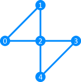
(a)

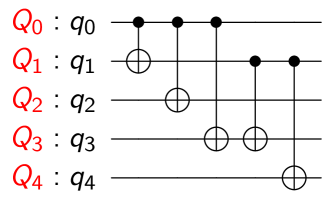
(b)

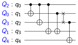
(c)

Figure 1: Compiling the 5 qubit circuit shown in (b) onto a 5 qubit device, namely ibmq_yorktown, whose coupling map is depicted in (a). The compiled circuit is shown in (c).

1.2 Our Contributions

In this paper, we present novel deterministic algorithms for compiling recurrent quantum circuit patterns in polynomial time. In particular, such patterns appear in quantum circuits that are used to compute the ground state properties of molecular systems using the variational quantum eigensolver (VQE) method together with the RyRz heuristic wavefunction Ansätz [18]. We implemented our algorithms in a Python software denoted as PADQC (PAttern-oriented Deterministic Quantum Compiler) that we integrated with Qiskit’s SABRE swapping strategy [19] and compilation routine [20], from now on denoted as Qiskit(SABRE).

We benchmarked PADQC+Qiskit(SABRE) using different quantum circuits, assuming IBM Quantum hardware. We show that our integrated solution produces – in general – output programs that are comparable to those obtained with state-of-art compilers, such as t$|$ket$\rangle$ [21], in terms of CNOT count and CNOT depth. In particular, our solution produces unmatched results on RyRz circuits.

The paper is organized as follows. In Section 2, we discuss the state of the art in quantum compiling. In Section 3, we present our algorithms. In Section 4, we illustrate the experimental evaluation of PADQC+Qiskit(SABRE). Finally, in Section 5, we conclude the paper with an outline of future work.

2 Related work

Recently, some noteworthy quantum compiling techniques have been proposed. Here we survey those that have been implemented into actual compilers, and benchmarked.

The approach proposed by Zulehner et al. [22] is to partition the circuit into layers, each layer including gates that can be executed in parallel. For each layer, a compliant CNOT mapping must be found, starting from an initial mapping obtained from the previous layer. Denoting the number of physical qubits as $m$ and the number of logical qubits as $n$, in the worst case there are $m!(m-n)!$ possible mappings. Such a huge search space cannot be explored exhaustively. The $A^{*}$ search algorithm is adopted, to find the less expensive swap sequence. Moreover, a lookahead strategy is adopted to minimize additional operations to switch between subsequent mappings. The proposed solution is efficient in terms of running time and output depth, but may not be scalable because of the exponential space complexity of the $A^{*}$ search algorithm [23].

SABRE by Li et al. [19] is a SWAP-based bidirectional heuristic search method. It requires a preprocessing phase consisting of the following steps. First of all, the distance matrix over the coupling map is computed. Then, the directed acyclic graph that represents the two-qubit gate dependencies of the circuit is generated. A data structure denoted as $F$ (front layer) is initialized as the set of two-qubit gates without unexecuted predecessors. The preprocessing phase ends up with the generation of a random initial mapping. Then, the compiling phase consists in iterating the following steps over $F$, until $F$ is empty. First, all executable gates are removed from $F$ and their successors are added to $F$. Second, for those gates in $F$ that cannot be executed, the best SWAP sequence is selected using an heuristic cost function based on distance matrix. Experiment results show that SABRE can generate hardware-compliant circuits with less or comparable overhead, with respect to the approach proposed by Zulehner et al. [22].

In Qiskit (version 0.20) [20], the compiling process is implemented by a customizable Pass Manager that schedules a number of different passes: layout selection, unrolling (i.e., gate synthesis), swap, gate optimization, and more. Four swap strategies are currently available: Basic, Stochastic, Lookahead and SABRE. The Stochastic strategy uses a randomized algorithm to map the input circuit to the selected coupling map. This means that a single run does not guarantee to produce the best result.

Currently, the most advanced quantum compiler is t$|$ket$\rangle$ [21], which is written in C++. The compiling process proceeds in two phases: an architecture-independent optimisation phase, which aims to reduce the size and complexity of the circuit; and an architecture-dependent phase, which prepares the circuit for execution on the target machine. The architecture-independent optimisation phase consists of peephole optimizations (targeting small circuit patterns) and macroscopic optimizations (aiming to identify high-level macroscopic structures in the circuit). The end product of this process is a circuit that can be scheduled for execution by the runtime environment, or simply saved for later.

In Section 4, we compare our PADQC+Qiskit(SABRE) integration with pure Qiskit(SABRE) and t$|$ket$\rangle$.

3 Algorithms

Most compiling approaches aim at finding a general purpose compiler, able to cope with any circuit without the possibility to make assumptions on its structure or characteristics. This kind of solution, although effective in many cases, may not be as much efficient when facing circuits characterized by well-defined peculiar sequences, i.e., patterns, of two-qubit operators. This is particularly true if those patterns repeat themselves many times in a circuit and are not compliant with the quantum device connectivity.

This is the case of RyRz circuits used to compute the ground state properties of molecular systems with the variational quantum eigensolver (VQE) method. These circuits were introduced for the first time in [18] as a heuristic hardware-efficient wavefunction Ansätz for the calculation of the electronic structure properties of small molecular systems such as hydrogen H₂, lithium hydride, LiH, and berillium hydride, BH₂, on a quantum computer. Contrary to other quantum circuits inspired by classical wavefunction expansion techniques (e.g., the coupled cluster expansion [24, 25]), in this case the nature of the circuit is solely motivated by the requirement of producing an entangled wavefunction for the many-electron systems that optimally fits the connectivity of the hardware at disposal. In most cases, the RyRz circuit offers a well balanced compromise between these two requirements. These circuits, when implemented with full entanglement (Fig. 2), are characterized by repeated sequences of a pattern that we denote as inverted CNOT cascade.

(d)

Figure 2: RyRz circuit example.

In Sections 3.2 and 3.3, we illustrate these patterns and how their features can be exploited to lay out efficient compiling algorithms. From now on, it will be assumed that the connectivity of the quantum device on which the circuit has to be compiled is similar to those featured by IBM Quantum devices [26] (Fig. 3). Table 1 presents an overview of the designed algorithms and their time complexity, which is computed by taking into account the worst case scenario and the running time of the subroutines.

The compilation process starts with Algorithm 1, which searches for patterns of interests and transforms them so that they are more easily mappable to the coupling map. Then, Algorithm 4 optimizes the circuit, removing double CNOTs and double H gates that may results from the previous transformations. Finally, Algorithm 5 finds a suitable initial mapping for the circuit.

Algorithm	Subroutines	Time Complexity
1 patterns	CheckCascade	$O(g)$
	CheckInverseCascade
2 CheckCascade		$O(m)$
3 CnotCancellation		$O(lm^{2})$
4 GateCancellation		$O(lm^{2})$
5 Chain	CheckForIsolated	$O(n)$
	ExpandChain
6 CheckForIsolated		$O(1)$
7 ExpandChain		$O(1)$

Table 1: Overview of proposed algorithms and their time complexity. Notation: $n$ is the number of qubits of the device, $m$ is the number of qubits used by the compiled circuit, $g$ is the number of gates in the circuit and $l$ the number of layers.

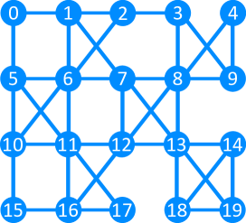
(a)

(b)

Figure 3: (a) 20 qubits ibmq_tokyo and (b) ibmq_almaden [26].

3.1 CNOT cascades

We are interested in the so called CNOT cascade, shown in Fig. 4. This pattern plays a prominent role in several quantum algorithms such as the one used to produce GHZ states [27, 28] as shown in Fig. 5.

The coupling maps in Fig. 3 prevent from placing all CNOT gates like in the ideal GHZ circuit, i.e., making a CNOT cascade where $n-1$ qubits control the nth qubit. It is indeed possible to turn the ideal GHZ circuit into an equivalent one characterized by a unique sequence of CNOT gates. It would only be a slight change to the technique discussed in a previous work [29].

However, this technique works only if the aim is to produce a GHZ state starting from a $|0\rangle^{\otimes n}$. This paper wants to focus on a more general case, where a CNOT cascade could appear at any point in the circuit and no assumption can be done on the state of the system.

(a)

(b)

Figure 4: (a) CNOT cascade. (b) Decomposition of a CNOT cascade

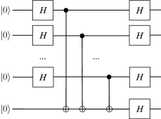
$\frac{\left|0\right\rangle^{\otimes n}+\left|1\right\rangle^{\otimes n}}{\sqrt{2}}$

Figure 5: GHZ circuit.

A possible solution is to exploit the nearest neighbor decomposition for a uniformly controlled gate studied by Tucci [30]. The only requirement for Tucci’s decomposition is that qubits are to be arranged in a linear chain.

To realize the decomposition in Fig. 4, Algorithm 1 analyzes the circuit layer by layer and, when a CNOT gate is encountered, Algorithm 2 checks if that CNOT is the first of a CNOT cascade. Each encountered CNOT cascade is replaced by its nearest-neighbor decomposition and, at the end, Algorithm 1 returns a new transformed circuit. Since Algorithm 1 just loops over all gates in a circuit, its complexity is $O(g)$ with $g$ being equal to the number of gates of the circuit.

Algorithm 1 Patterns($circuit$)
Input: a quantum circuit $circuit$
Output: a new transformed circuit

1:  $new\_circuit\leftarrow\emptyset$

2:  to_skip $\leftarrow\emptyset$

3:  new_layers $\leftarrow[\emptyset\textbf{ for }0\leq i<|circuit\_layers|]$

4:  for $i=0$ to $|circuit\_layers|$ do

5:     if $i\neq 0$ then

6:        for all $g\in$ new_layers[$i-1$] do

7:           put g into new_circuit

8:        end for

9:     end if

10:     for all $gate\in circuit\_layers[i]$ do

11:        if $gate\not\in$ to_skip then

12:           if gate is CNOT then

13:              transformed $\leftarrow$ CheckCascade($circuit\_layers$, $i$, new_layers)

14:              if trasnformed $\neq\emptyset$ then

15:                 put transformed into to_skip

16:                 continue

17:              else

18:                 put $gate$ into to_skip

19:                 put gate into new_circuit

20:              end if

21:           else

22:              put $gate$ into to_skip

23:              put gate into new_circuit

24:           end if

25:        end if

26:     end for

27:  end for

28:  return  new_circuit

Algorithm 2 analyzes the circuit starting from a CNOT gate; here before and after are sets of gates that can be applied before and after the decomposition. If a CNOT cascade is found, the decomposition is applied between the before and after gates sets, otherwise an empty set is returned. In Algorithm 2, $gate_{t}$ is the target of $gate$ and if $gate$ is a CNOT, $gate_{c}$ is the control qubit of $gate$. As it is expected that cascades are no longer than the number of qubits in the circuit, the algorithm stops when, after $MAX=2m$ layers have been checked, no pattern is found. The time complexity of Algorithm 2 is $O(m)$. Usually the number of gates $g$ is greater than $m$, thus, the complexity of Algorithm 1 is $O(g)$.

Algorithm 2 CheckCascade($layers$, $i$, $new\_layers$)
Input: the list of layers in the circuit $layers$; the layer from where to start $i$; the list of $new\_layers$ to be added
Output: the list of gates to skip, $\emptyset$ if no cascade was found

1:  before $\leftarrow\emptyset$, after $\leftarrow\emptyset$, skip $\leftarrow\emptyset$, off_limits $\leftarrow\emptyset$, control $\leftarrow cnot_{c}$, target $\leftarrow cnot_{t}$, used $\leftarrow\emptyset$, found $\leftarrow$ false, ctrls $\leftarrow\emptyset$, put target into used, $i\leftarrow 0$, $gate\leftarrow circuit[0]$, $c\leftarrow 0$, last $\leftarrow i$

2:  while $i<MAX$ do

3:     for all $gate\in layers[i+c]$ do

4:        if $gate\in$ skip and $gate_{t}=$ target then

5:           $c\leftarrow MAX$

6:           break

7:        else

8:           if $gate$ is a CNOT then

9:              if $gate_{c}=$ target then

10:                 $count\leftarrow MAX$

11:                 break

12:              else if $gate_{c}\in$ off_limits or $gate_{t}\in$ off_limits then

13:                 put $gate_{c}$ into off_limits

14:                 put $gate_{c}$ into used

15:                 put $gate_{t}$ into off_limits

16:                 put $gate_{t}$ into used

17:                 continue

18:              end if

19:              if $gate_{t}=$ target and $gate_{c}\not\in$ ctrls and $gate_{c}\not\in$ used then

20:                 put $gate_{c}$ into ctrls

21:                 put $gate_{c}$ into used

22:                 put $gate$ into skip

23:              else if $gate_{t}\neq$ target and $gate_{c}\neq$ target then

24:                 if $gate_{t}\not\in$ used and $gate_{c}\not\in$ used and last $<c$ then

25:                    last $\leftarrow i+c$

26:                 else

27:                    put $gate_{c}$      into off_limits

28:                    put $gate_{c}$      into used

29:                    put $gate_{t}$      into off_limits

30:                    put $gate_{t}$      into used

31:                    if last $>i+c-1$ then

32:                       last $\leftarrow i+c-1$

33:                    end if

34:                 end if

35:              else

36:                 $count\leftarrow MAX$

37:                 break

38:              end if

39:           else

40:              if $gate_{t}\in$ off_limits then

41:                 continue

42:              else if $gate_{t}=$ target then

43:                 put $gate$ into after

44:                 put $gate$ into skip

45:                 $c\leftarrow MAX$

46:                 break

47:              else if $gate_{t}\not\in$ used then

48:                 put $gate$ into before

49:              else

50:                 put $gate$ into after

51:              end if

52:              put $gate$ into skip

53:           end if

54:        end if

55:     end for

56:     $c\leftarrow c+1$

57:  end while

58:  if $|$controls$|>1$ then

59:     for all g $\in$ before do

60:        put g into $new\_layers[$last$]$

61:     end for

62:     for all $x\in$ reversed(ctrls) $\cup$ target do

63:        put $cnot_{x,x.next}$      into $new\_layers[$last$]$

64:     end for

65:     for all $y\in$ ctrls do

66:        put $cnot_{y,y.next}$      into $new\_layers[$last$]$

67:     end for

68:     for all g $\in$ after do

69:        put g into $new\_layers[$last$]$

70:     end for

71:     return  skip

72:  end if

73:  return  $\emptyset$

We recall that the aim is to compile circuits characterized by repeated patterns. Let us look at the circuit in Fig. 6, where multiple CNOT cascades are repeated one after the other, acting on different target qubits. Algorithm 1 outputs the circuit in Fig. 6, which despite being correct, has an increased depth.

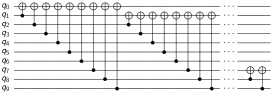
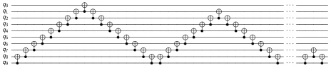
(a)
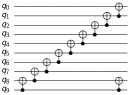
(b)	(c)

Figure 6: (a) Circuit with multiple CNOT cascades. (b) Circuit after nearest-neighbor decomposition. (c) Circuit after CNOT cancellation.

Fortunately, if two consecutive CNOT gates act on the same control and target qubit, they elide each other, as a CNOT gate is the inverse gate of itself. Algorithm 3 loops over the circuit to cancel double CNOT gates until no further cancellation can be done.

Since each layer in the circuit has at most $m$ gates, in the worst case Algorithm 3 needs $m$ iterations to cancel every CNOT couple. Its time complexity is $O(lm^{2})$, where $l$ is the number of layers and usually $m\ll l$.

Algorithm 3 CnotCancellation($circuit$)
Input: a quantum circuit $circuit$
Output: a new circuit without double CNOTs

1:  changed $\leftarrow$ true

2:  while changed is true do

3:     changed $\leftarrow$ false

4:     for all $layer\in circuit$ do

5:        for all $gate\in layer$ do

6:           if $gate$ is cnot then

7:              if $cnot_{gate_{c},gate_{t}}\in layer.next$ then

8:                 remove gate from layer

9:                 remove $cnot_{gate_{c},gate_{t}}$ from layer.next

10:                 changed $\leftarrow$ true

11:              end if

12:           end if

13:        end for

14:     end for

15:  end while

The result of such an optimization is shown in Fig. 6. This new optimized circuit has a much more acceptable depth, even lower than the original circuit shown in Fig. 6.

3.2 Inverted CNOT cascades

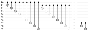
Figure 7: Circuit with multiple inverse CNOT cascades.

The pattern characterizing RyRz circuits, shown in Fig. 7, is very similar to the one in Fig. 4. Indeed this pattern can be turned into the other one by inverting all of its CNOT gates by means of H gates on both control and target qubits before and after the CNOT. Of course adding H gates to invert a CNOT would alter the circuit identity, therefore, instead of adding an H gate, two H gates are added so that they can negate each other’s effects and leave the circuit identity untouched. The result of this operation is shown in Fig. 8.

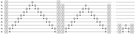
(a)
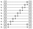
(b)	(c)

Figure 8: (a) Circuit with multiple inverse CNOT cascades after CNOT inversion. (b) Circuit with multiple inverse CNOT cascades after nearest-neighbor decomposition. (c) Circuit with multiple inverse CNOT cascades after gates cancellation.

Using an algorithm similar to Algorithm 2, with the roles of control and target qubits exchanged, and a slight modification to Algorithm 1, the circuit in Fig. 8 can be compiled obtaining the one in Fig. 8. Algorithm 4 optimizes the circuit producing the one shown in Fig. 8. Like in the previous case, the depth of the recompiled circuit is very close to the original. The time complexity of Algorithm 4 is $O(lm^{2})$.

Algorithm 4 GateCancellation($circuit$)
Input: $circuit$ a quantum circuit
Output: a new circuit without double CNOTs and double H

1:  changed $\leftarrow$ true

2:  while changed is true do

3:     changed $\leftarrow$ false

4:     for all $layer\in circuit$ do

5:        for all $gate\in layer$ do

6:           if $gate$ is cnot then

7:              if $cnot_{gate_{c},gate_{t}}\in layer.next$ then

8:                 remove gate from layer

9:                 remove $cnot_{gate_{c},gate_{t}}$ from layer.next

10:                 changed $\leftarrow$ true

11:              end if

12:           else if $gate$ is $H$ then

13:              if $gate\in layer.next$ then

14:                 remove $gate$ from layer

15:                 remove $gate$ from layer.next

16:                 changed $\leftarrow$ true

17:              end if

18:           end if

19:        end for

20:     end for

21:  end while

3.3 Nearest neighbor CNOT sequences

In the previous section we showed how to transform inverted CNOT cascades into nearest-neighbor CNOT sequences. Clearly such a sequence of gates, where every qubit $q_{i}$ controls $q_{i+1}$, cannot be directly executed on the coupling map in Fig. 3, as $q_{i}$ is not always connected with $q_{i+1}$.

A possible solution is to find a path in the coupling map such that every qubit $q_{i}$, with $1<i<n-1$, with $n$ being the number of qubits in the device, has a connection with its nearest neighbors $q_{i-1}$ and $q_{i+1}$. This is related to the problem of finding an Hamiltonian path, i.e., a path that visits each vertex of a graph exactly once. The Hamiltonian path problem is a special case of the Hamiltonian cycle problem and is known to be NP-Complete, in fact it is an instance of the famous traveling salesman problem [31].

Fortunately, one can take advantage of the features of the coupling map such as its regular structure and the fact that every qubit is identified by a number ranging from $0$ to $n$. As each undirected link can be seen as a couple of ingoing and outgoing links, the path obtained resembles a chain and will be denoted as such, from now on.

Algorithm 5 computes a chain in an undirected graph $\mathcal{G}$ starting from node $0$, where $\mathcal{C}$ is the chain initialized as empty, $\mathcal{S}$ is the set of nodes to be explored and $\mathcal{N}_{x}$ is the set of neighbors of node $x$. The algorithm loops over the nodes until the set of explored nodes $\mathcal{E}$ is equal to the set of nodes in $\mathcal{G}$. For every node added to $\mathcal{C}$, the chain() algorithm checks if the node’s neighbors lead to a dead end, i.e., are isolated. If one neighbor is found to be isolated, it is added to the set of isolated nodes $\mathcal{I}$ and also to $\mathcal{E}$.

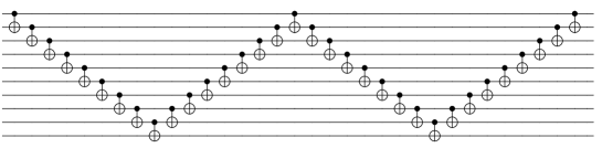
Figure 9: Circuit with nearest neighbor CNOT sequences.

Algorithm 5 Chain($\mathcal{G}$, $n$)
Input: undirected graph $\mathcal{G}$; number of qubits $n$ used by the circuit
Output: a chain $C$ connecting at least $n$ nodes in $\mathcal{G}$

1:  $\mathcal{C}\leftarrow\emptyset$

2:  $\mathcal{S}\leftarrow$ all nodes of $\mathcal{G}$

3:  put $0$ into $\mathcal{C}$

4:  $\mathcal{S}\leftarrow\mathcal{S}/0$

5:  $\mathcal{E}\leftarrow 0$

6:  $\mathcal{I}\leftarrow\emptyset$

7:  $x=\mathcal{C}[|\mathcal{C}|-1]$

8:  $last\_back\_step\leftarrow-1$

9:  while $|\mathcal{E}|<|\mathcal{G}|$ do

10:     $\mathcal{N}\leftarrow\mathcal{N}_{x}/E$

11:     if $|\mathcal{N}|\neq\emptyset$ then

12:        if $x+1\in\mathcal{N}_{x}$ then

13:           $x\leftarrow x+1$

14:        else

15:           $x\leftarrow min(\mathcal{N}_{x})$

16:        end if

17:        put $x$ into $\mathcal{E}$

18:        put $x$ into $\mathcal{C}$

19:        $\mathcal{S}\leftarrow\mathcal{S}/x$

20:        if $|\mathcal{E}|<|\mathcal{G}|-1$ then

21:           $\mathcal{N}\leftarrow\emptyset$

22:           for all $q\in\mathcal{N}_{x}$ do

23:              if $q\not\in\mathcal{E}$ then

24:                 remove=true

25:                 if $|N_{q}|=1$ and $|\mathcal{E}<|G|-1|$ then

26:                    put $q$ into $\mathcal{E}$

27:                    $\mathcal{S}\leftarrow\mathcal{S}/q$

28:                    put $q$ into $\mathcal{I}$

29:                    continue

30:                 end if

31:                 for all $r\in\mathcal{N}_{q}$ do

32:                    if $r\not\in\mathcal{E}$ and $r=x$ then

33:                       remove=false

34:                    end if

35:                    if remove=true then

36:                       put $q$ into $\mathcal{E}$

37:                       $\mathcal{S}\leftarrow\mathcal{S}/q$

38:                       put $q$ into $\mathcal{I}$

39:                    end if

40:                 end for

41:              end if

42:           end for

43:        end if

44:     else

45:        if $last\_back\_step\neq\mathcal{C}[|\mathcal{C}|-2]$ and $|\mathcal{G}|-|\mathcal{E}|>|current-\mathcal{S}[0]|$ then

46:           break

47:        end if

48:        put $x$ into $\mathcal{I}$

49:        $\mathcal{C}\leftarrow\mathcal{C}/x$

50:        $x\leftarrow\mathcal{C}[|\mathcal{C}|-1]$

51:        $last\_back\_step\leftarrow x$

52:     end if

53:  end while

54:  if $|\mathcal{C}|\geq n$ then

55:     return  $\mathcal{C}$

56:  end if

57:  CheckForIsolated($\mathcal{G}$, $\mathcal{C}$, $\mathcal{E}$, $\mathcal{I}$)

58:  ExpandChain($\mathcal{G}$, $\mathcal{C}$, $\mathcal{I}$, $n$)

59:  return  $\mathcal{C}$

After executing Algorithm 5 on the coupling map in Fig. 3, the path obtained can be used to formulate an initial layout for the circuit in Fig. 9, such that logical qubit $q_{i}$ corresponds to chain element $\mathcal{C}[i]$. Fig. 10 shows the path obtained in the coupling map highlighted in red. Such an initial layout eliminates the need to use SWAP gates and produces a circuit with ideally no increase in depth.

Figure 10: Qubit chain in ibmq_almaden highlighted in red.

Algorithm 6 CheckForIsolated($\mathcal{G}$, $\mathcal{C}$, $\mathcal{E}$, $\mathcal{I}$)
Input: an undirected graph $\mathcal{G}$; $\mathcal{C}$ a chain of nodes in $\mathcal{G}$; $\mathcal{E}$ nodes already explored; $\mathcal{I}$ nodes left outside $\mathcal{C}$ during exploration

1:  for $m=0$ to $|\mathcal{G}|-1$ do

2:     if $m\not\in\mathcal{E}$ and $m\not\in\mathcal{I}$ then

3:        for all $i\in\mathcal{I}$ do

4:           if $m\in\mathcal{N}_{i}$ then

5:              put $m$ into $\mathcal{I}$

6:              put $m$ into $\mathcal{E}$

7:              break

8:           end if

9:        end for

10:        for all $n\in\mathcal{N}_{m}$ do

11:           if $n\in\mathcal{C}$ then

12:              put $m$ into $\mathcal{I}$

13:              put $m$ into $\mathcal{E}$

14:              break

15:           end if

16:        end for

17:     end if

18:  end for

Algorithm 7 ExpandChain($\mathcal{G}$, $\mathcal{C}$, $\mathcal{I}$, $n$)
Input: an undirected graph $\mathcal{G}$; $\mathcal{C}$ a chain of nodes in $\mathcal{G}$; $\mathcal{I}$ nodes left outside $\mathcal{C}$ during exploration; $n$ the number of qubits used by the circuit

1:  $r\leftarrow(n-|\mathcal{C}|)$

2:  while $r>0$ do

3:     for all $m\in\mathcal{I}$ do

4:        $x\leftarrow min(\mathcal{N}_{m}\cap\mathcal{C})$

5:        if $x\neq\emptyset$ then

6:           put $m$ into $\mathcal{C}$ after $x$

7:           $\mathcal{I}\leftarrow\mathcal{I}/m$

8:           $r\leftarrow r-1$

9:           break

10:        end if

11:     end for

12:  end while

Nodes $4$ and $15$ are left outside the chain as it is already sufficiently long, to map the circuit in Fig. 9, and adding these two extra qubits would require the use of SWAP gates during compilation. For a larger circuit, then those nodes will be inserted in the chain in a suitable position (nodes $4$ between $3$ and $8$, node $15$ between $16$ and $17$). Cycling through all $n$ nodes in the map, the time complexity of Algorithm 5 is $O(n)$.

4 Experimental results

We implemented the algorithms presented in Section 3 in a quantum compiler written in Python language, denoted as PADQC. In the PADQC framework, quantum circuits are represented by QCircuit objects, which are based on the well known formalism of Directed Acyclic Graphs (DAGs). In DAGs, nodes represent quantum gates and the edges connecting them correspond to qubits and bits. A QCircuit can then be easily converted into Open QASM [32] and vice versa, allowing PADQC to interact with Qiskit.

		CNOT Gate Count
			ibmq_tokyo			ibmq_almaden
Circuit Name	n	Initial	Qiskit(SABRE)	PADQC+Qiskit(SABRE)	t$|$ket$\rangle$	Qiskit(SABRE)	PADQC+Qiskit(SABRE)	t$|$ket$\rangle$
H2_RYRZ	4	30	30	21	30	60	21	70
LiH_RYRZ	12	330	788	101	898	1256	101	1260
H2O_RYRZ	14	455	1242	121	1301	1763	121	1738
Random_20q_RYRZ	20	950	2735	182	3053	3976	201	4146

Table 2: Circuit CNOT gate count of the compiled quantum chemistry circuits, considering the ibmq_tokyo and ibmq_almaden architectures.

		CNOT Depth
			ibmq_tokyo			ibmq_almaden
Circuit Name	n	Initial	Qiskit(SABRE)	PADQC+Qiskit(SABRE)	t$|$ket$\rangle$	Qiskit(SABRE)	PADQC+Qiskit(SABRE)	t$|$ket$\rangle$
H2_RYRZ	4	21	21	21	21	60	21	70
LiH_RYRZ	12	69	488	101	575	648	101	703
H2O_RYRZ	14	81	675	121	813	846	121	875
Random_20q_RYRZ	20	117	1361	182	1648	1562	201	1629

Table 3: Circuit CNOT depth of the compiled quantum chemistry circuits, considering the ibmq_tokyo and ibmq_almaden architectures.

Using an Intel Xeon E5-2683v4 2.1GHz with 50 GB of RAM, we benchmarked the quantum compiler with different quantum circuits. In particular, we considered a few quantum chemistry circuits for the RyRz heuristic [18] wavefunction Ansätz (Fig. 2), and an heterogeneous set of quantum circuits that has been used in most reference works [19, 22]. We assumed IBM Quantum hardware, namely ibmq_tokyo and ibmq_almaden architectures. They both have 20 qubits, but their coupling maps are quite different (Fig. 3).

We compared Qiskit(SABRE) with t$|$ket$\rangle$ and Qiskit(SABRE) preceded by PADQC transformations and mapping. Given that on NISQ devices multi-qubit operations tend to have error rates and execution times an order of magnitude worse than single-qubit ones [33], the performance indicators used are CNOT gate gate count and CNOT depth of the circuit, i.e., the depth of the circuit taking into account only CNOT gates. As shown in Table 2 and Table 3, the combination of PADQC and Qiskit(SABRE) outperforms both Qiskit(SABRE) alone and t$|$ket$\rangle$ on all RyRz circuits tested, regardless of the considered architecture.

We also tested PADQC on a larger set of circuits. We compiled a total of 190 circuits, taken from RevLib [34], Quipper [35] and Scaffold [36], plus the quantum chemistry ones. The results are summarized in Fig. 11 to 12, where the initial value of the considered metric is on the x-axis and the value for the compiled circuit on the y-axis.

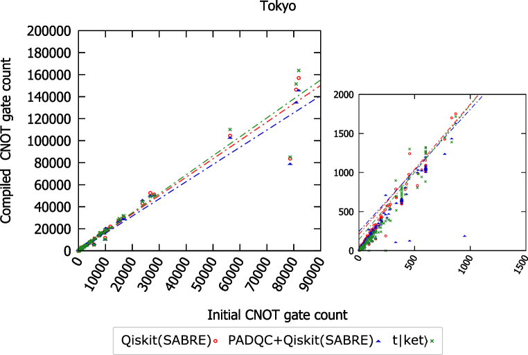
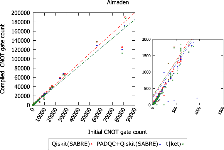
Figure 11: Comparing the CNOT gate count of the circuits compiled on ibmq_tokyo and ibmq_almaden.

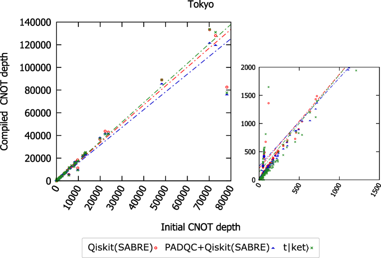
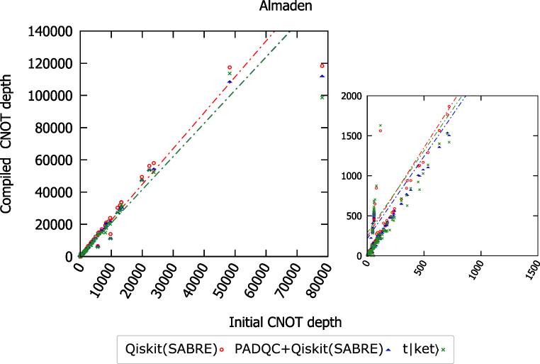
Figure 12: Comparing the CNOT depth of the circuits compiled on ibmq_tokyo and ibmq_almaden.

When compiling on the ibmq_tokyo architecture, we can see, with the help of tendency lines calculated using the least squares method, that the combination of PADQC and Qiskit(SABRE) not only boosts Qiskit(SABRE) performance but can also compete with t$|$ket$\rangle$. As we switch to the less connected ibmq_almaden architecture, PADQC can still boost Qiskit(SABRE) performance while being up to par with t$|$ket$\rangle$.

5 Conclusion

In this paper, we proposed novel deterministic algorithms for compiling recurrent quantum circuit patterns in polynomial time. Starting from this set of algorithms, we have implemented PADQC, which has two main features. First, it identifies CNOT cascades and exploits useful circuit identities to transform them into CNOT nearest-neighbor sequences. Second, it finds an initial mapping that can comply with circuits characterized by recurrent CNOT nearest-neighbor sequences. Finally, we integrated PADQC with Qiskit’s SABRE swapping strategy and compilation routine.

We illustrated the results of the experimental evaluation of our integrated solution using different quantum programs and assuming IBM Quantum hardware. Among others, we compiled quantum circuits that are used to compute the ground state properties of molecular systems using the VQE method together with the RyRz heuristic wavefunction Ansätz. PADQC+Qiskit(SABRE), in general, produces output programs that are on par with those produced by state-of-art tools, in terms of CNOT count and CNOT depth. In particular, our solution produces unmatched results on RyRz circuits.

In future work, we plan to expand PADQC to other patterns of interests and look for further circuit identities as the one found between nearest-neighbor CNOT sequences and CNOT cascade. These identities proved to be crucial in the quest for optimal quantum compilation. Moreover, we will investigate to possibility of integrating PADQC pattern transformation and mapping algorithms with alternative swapping strategies, which could produce an appreciable performance improvement.

While effective, CNOT count and CNOT depth are only pseudo-objectives. What really matters is the fidelity of a computation when run on actual quantum hardware. We believe that the proposed compiler could be enhanced with noise related information (such as gate error rates and decoherence times) with the aim of finding a good trade-off between circuit depth and computation fidelity.

References

- [1] R. P. Feynman. Simulating physics with computers. International Journal of Theoretical Physics, 21(6-7):467–488, 1982.
- [2] P. W. Shor. Algorithms for quantum computation: discrete logarithms and factoring. In Proceedings 35th Annual Symposium on Foundations of Computer Science, pages 124–134, 1994.
- [3] A. Chiesa, F. Tacchino, M. Grossi, P. Santini, I. Tavernelli, D. Gerace, and S. Carretta. Quantum hardware simulating four-dimensional inelastic neutron scattering. Nature Physics, 15:455–459, 2019.
- [4] S. Lloyd, M. Mohseni, and P. Rebentrost. Quantum principal component analysis. Nature Physics, 10(9):631–633, 2014.
- [5] Jacob Biamonte, Peter Wittek, Nicola Pancotti, Patrick Rebentrost, Nathan Wiebe, and Seth Lloyd. Quantum machine learning. Nature, 549(7671), September 2017.
- [6] Vojtěch Havlíček, Antonio D. Córcoles, Kristan Temme, Aram W. Harrow, Abhinav Kandala, Jerry M. Chow, and Jay M. Gambetta. Supervised learning with quantum-enhanced feature spaces. Nature, 567(7747):209–212, March 2019.
- [7] Christa Zoufal, Aurélien Lucchi, and Stefan Woerner. Quantum Generative Adversarial Networks for learning and loading random distributions. npj Quantum Information, 5(1):1–9, November 2019.
- [8] Iris Cong, Soonwon Choi, and Mikhail D. Lukin. Quantum convolutional neural networks. Nature Physics, 15(12), December 2019.
- [9] F. Tacchino, C. Macchiavello, D. Gerace, and D. Bajoni. An artificial neuron implemented on an actual quantum processor. NPJ Quantum Information, 5:26:1–8, 2019.
- [10] A. K. Ekert. Quantum cryptography based on Bell’s theorem. Phys. Rev. Lett., 67:661–663, 1991.
- [11] C. Portmann and R. Renner. Cryptographic security of quantum key distribution. arxiv:1409.3525, 2014.
- [12] Joseph F. Fitzsimons. Private quantum computation: an introduction to blind quantum computing and related protocols. npj Quantum Information, 3(1), June 2017.
- [13] A. D. Córcoles, A. Kandala, A. Javadi-Abhari, D. T. McClure, A. W. Cross, K. Temme, P. D. Nation, M. Steffen, and J. M. Gambetta. Challenges and opportunities of near-term quantum computing systems. Proceedings of the IEEE, 108(8):1338–1352, 2020.
- [14] A. Botea, A. Kishimoto, and R. Marinescu. On the Complexity of Quantum Circuit Compilation. In The Eleventh International Symposium on Combinatorial Search (SOCS 2018), 2018.
- [15] M. Soeken, G. Meuli, B. Schmitt, F. Mozafari, H. Riener, and G. De Micheli. Boolean satisfiability in quantum compilation. Phil. Trans. Royal Soc. A, 378(2164):1–16, 2019.
- [16] V. Kliuchnikov, D. Maslov, and M. Mosca. Practical Approximation of Single-Qubit Unitaries by Single-Qubit Quantum Clifford and T Circuits. IEEE Transactions on Computers, 65(1):161–172, 2016.
- [17] E. Munoz-Coreas and H. Thapliyal. Quantum circuit design of a T-count optimized integer multiplier. IEEE Transactions on Computers, 68(5):729–739, 2019.
- [18] Abhinav Kandala, Antonio Mezzacapo, Kristan Temme, Maika Takita, Markus Brink, Jerry M. Chow, and Jay M. Gambetta. Hardware-efficient variational quantum eigensolver for small molecules and quantum magnets. Nature, 549(7671):242–246, September 2017.
- [19] Gushu Li, Yufei Ding, and Yuan Xie. Tackling the qubit mapping problem for nisq-era quantum devices. In Proceedings of the Twenty-Fourth International Conference on Architectural Support for Programming Languages and Operating Systems, ASPLOS ’19, page 1001–1014, 2019.
- [20] Héctor Abraham et al. Qiskit: An open-source framework for quantum computing, 2019.
- [21] Seyon Sivarajah, Silas Dilkes, Alexander Cowtan, Will Simmons, Alec Edgington, and Ross Duncan. tket: a retargetable compiler for NISQ devices. Quantum Science and Technology, 6(1):014003, 2020.
- [22] Alwin Zulehner, Alexandru Paler, and Robert Wille. An efficient methodology for mapping quantum circuits to the IBM QX architectures. IEEE Trans. on CAD of Integrated Circuits and Systems, 38(7):1226–1236, 2019.
- [23] S. Russell and P. Norvig. Artificial Intelligence: A Modern Approach 4th Edition. Pearson, 2020.
- [24] A. Peruzzo, J. McClean, P. Shadbolt, M.-H. Yung, X.-Q. Zhou, P. J. Love, A. Aspuru-Guzik, and J. L. O’Brien. A variational eigenvalue solver on a photonic quantum processor. Nature Communications, 5(4213):1–7, 2014.
- [25] Panagiotis Kl. Barkoutsos, Jerome F. Gonthier, Igor Sokolov, Nikolaj Moll, Gian Salis, Andreas Fuhrer, Marc Ganzhorn, Daniel J. Egger, Matthias Troyer, Antonio Mezzacapo, Stefan Filipp, and Ivano Tavernelli. Quantum algorithms for electronic structure calculations: Particle-hole Hamiltonian and optimized wave-function expansions. Phys. Rev. A, 98:022322, Aug 2018.
- [26] IBM. Quantum computation center opens.
- [27] D. M. Greenberger, M. A. Horne, and A. Zeilinger. Going beyond bell’s theorem. In M. Kafatos, editor, Bell’s Theorem, Quantum Theory, and Conceptions of the Universe, pages 69–72. Kluwer Academic Publishers, 1989.
- [28] S. Deffner. Demonstration of entanglement assisted invariance on IBM’s quantum experience. Heliyon, 3(11), 2017.
- [29] D. Ferrari and M. Amoretti. Efficient and effective quantum compiling for entanglement-based machine learning on ibm q devices. International Journal of Quantum Information, 16(08), 2018.
- [30] Robert R. Tucci. QC Paulinesia. arxiv:0407215, July 2004.
- [31] C. H. Papadimitriou and K. Steiglitz. Combinatorial Optimization: Algorithms and Complexity. Dover Books on Computer Science. Dover Publications, 1998.
- [32] Andrew W. Cross, Lev S. Bishop, John A. Smolin, and Jay M. Gambetta. Open Quantum Assembly Language. arxiv:1707.03429, 2017.
- [33] Frank Arute, Kunal Arya, Ryan Babbush, Dave Bacon, et al. Quantum supremacy using a programmable superconducting processor. Nature, 574(7779):505–510, Oct 2019.
- [34] R. Wille, D. Große, L. Teuber, G. W. Dueck, and R. Drechsler. Revlib: An online resource for reversible functions and reversible circuits. In 38th International Symposium on Multiple Valued Logic (ismvl 2008), pages 220–225, 2008. RevLib is available at http://www.revlib.org.
- [35] Alexander S. Green, Peter FqiskiLeFanu Lumsdaine, Neil J. Ross, Peter Selinger, and Benoît Valiron. Quipper: A scalable quantum programming language. SIGPLAN Not., 48(6):333–342, June 2013.
- [36] Ali JavadiAbhari, Shruti Patil, Daniel Kudrow, Jeff Heckey, Alexey Lvov, Frederic T. Chong, and Margaret Martonosi. Scaffcc: Scalable compilation and analysis of quantum programs. Parallel Computing, 45:2 – 17, 2015. Computing Frontiers 2014: Best Papers.