Field-induced valence fluctuations in YbB₁₂

Abstract

We performed high-magnetic-field ultrasonic experiments on YbB₁₂ up to 59 T to investigate the valence fluctuations in Yb ions. In zero field, the longitudinal elastic constant $C_{11}$, the transverse elastic constants $C_{44}$ and $\left(C_{11}-C_{12}\right)/2$, and the bulk modulus $C_{\mathrm{B}}$ show a hardening with a change of curvature at around 35 K indicating a small contribution of valence fluctuations to the elastic constants. When high magnetic fields are applied at low temperatures, $C_{\mathrm{B}}$ exhibits a softening above a field-induced insulator-metal transition signaling field-induced valence fluctuations. Furthermore, at elevated temperatures, the field-induced softening of $C_{\mathrm{B}}$ takes place at even lower fields and $C_{\mathrm{B}}$ decreases continuously with field. Our analysis using the multipole susceptibility based on a two-band model reveals that the softening of $C_{\mathrm{B}}$ originates from the enhancement of multipole-strain interaction in addition to the decrease of the insulator energy gap. This analysis indicates that field-induced valence fluctuations of Yb cause the instability of the bulk modulus $C_{\mathrm{B}}$.

I Introduction

Since the electronic and magnetic properties of materials are mainly determined by valence electrons, a precise knowledge about the valence state is important in material science. Especially for $4f$-electron systems, the valence determines the total angular momentum $J$, the localized (or delocalized) $4f$-electron character, and corresponding wave functions. A non-integer valence state appears in some rare-earth compounds with Ce, Sm, Eu, and Yb ions. In such materials, valence fluctuations due to hybridization between conduction electrons and $4f$ electrons play a key role in their physical properties. YbB₁₂ is one of the valence fluctuating materials with such a $c$-$f$ hybridization, a high-Kondo temperature, and insulating character Kasaya_JMMM31 ; Susaki_PRL77 .

YbB₁₂ has the UB₁₂-type crystal structure belonging to the $Fm\overline{3}m$ ($O_{h}^{5}$) space group Kasaya_JMMM31 . The $\Gamma_{8}$ ground state of the $4f$ electrons based on Yb³⁺ configuration in the crystal electric field (CEF) has been proposed Nemkovski_PRL99 ; Kanai_JPSJ84 . The almost degenerated $\Gamma_{7}$ and the $\Gamma_{6}$ states at 270 K (23 meV) were considered as excited states Nemkovski_PRL99 ; Kanai_JPSJ84 . These CEF states based on the $J=7/2$ can be consistent with the hyperfine coupling constant for free Yb³⁺ ions determined by NMR measurements Ikushima_PhysB281 . In contrast, a nonmagnetic ground state has been suggested from the temperature-independent magnetic susceptibility at low temperatures Kasaya_JMMM47 ; Iga_JMMM177 . Indication for a strongly hybridized electronic state was found using bulk-sensitive x-ray photoelectron spectroscopy showing a slight deviation from the valence Yb³⁺ Yamaguchi_PRB79 . The hybridization between $5d$ conduction electrons and $4f$ localized electrons has been proposed as a candidate mechanism for an observed band-gap opening Saso_JPSJ72 ; Ohashi_PRB70 . The contribution of the B-$2p$ electrons to the $c$-$f$ hybridization is also discussed as a result of $dd\sigma$ hopping through B₁₂ clusters.

In addition to the CEF scheme, several characteristic energies related to the insulating character have been studied in YbB₁₂. Both in a polycrystal and single crystal, resistivity measurements show evidence for two activation energies of $\sim$ 30 and 65 K Kasaya_JMMM47 ; Iga_JMMM177 . A density of states with two-double peaks was proposed as a mechanism of two activation energies Sugiyama_JPSJ57 . NMR and specific-heat data have been described by a simple two-band model, each band having a bandwidth of 55 K, and with an energy gap of 140 K at the Fermi energy Kasaya_JMMM47 ; Iga_JMMM76 . High-resolution photoemission spectroscopy suggested a hybridization gap of 170 K (15 meV) below 150 K and strongly hybridized character below 60 K Takeda_PRB73 .

In YbB₁₂, various high-magnetic-field studies were performed to elucidate the mechanism of the formation of the energy gap. High-field magnetoresistance measurements indicated that the energy gap of 30 K closes around 45 T while the other gap remains up to higher fields Sugiyama_JPSJ57 . Magnetization measurements revealed metamagnetic behavior at insulator-metal (IM) transitions at $B_{\mathrm{IM}}=47$ T for $B\|[001]$ and 54 T for $B\|[110]$ and $B\|[111]$ Iga_JPhysConfSer200 . Another magnetization anomaly indicating the saturation of magnetization appears at 102 T Terashima_JPSJ86 . The energy shift of the $4f$ band due to the Zeeman effect was proposed to explain the closing of the band gap of 170 K. Synchrotron x-ray absorption spectra showed the field independence of the $L_{3}$ edge indicating no considerable change of the Yb valence in the field-induced metal phase Matsuda_JPhys51 . Specific-heat measurements revealed a discontinuous enhanced of Sommerfeld coefficient, $\gamma\sim 60$ mJ/mol$\cdot$K², and a corresponding Kondo temperature of $220$ - $250$ K above the IM transition, suggesting that the high-field phase is a valence-fluctuating Kondo metal Terashima_PRL120 . These high-field experiments indicate a contribution of the $c$-$f$ hybridization to the opening of the energy gap in YbB₁₂. Magnetic quantum oscillations in the insulating phase have also been focused to understand the insulating character of YbB₁₂ Xiang_Science362 .

To further investigate the valence fluctuations caused by the $c$-$f$ hybridization in YbB₁₂, we focused on ultrasonic measurement. Since a valence change causes an isotropic change of the ionic radii, an isotropic volume change of the crystal lattice is induced and the CEF Hamiltonian, $H_{\mathrm{CEF}}$, of Eq. (10) (see Appendix B) is changed to $H_{\mathrm{CEF}}+(\partial H_{\mathrm{CEF}}/\partial\varepsilon_{\mathrm{B}})\varepsilon_{\mathrm{B}}$. Here, $\varepsilon_{\mathrm{B}}$ is the volume strain with the irreducible representation (irrep) $\Gamma_{1}$ of the $O_{h}$ symmetry. This additional term to the CEF is described as a coupling between $\varepsilon_{\mathrm{B}}$ and a hexadecapole $H_{0}$ with $\Gamma_{1}$ in YbB₁₂. The schematic view of $\varepsilon_{\mathrm{B}}$ and $H_{0}$ in YbB₁₂ are shown in Figs. 1(a) and 1(b), respectively. Based on simple Landau theory for elasticity, the total free energy consists of a lattice and an electronic part is given by Luthi Phys. Ac.

$$F=\frac{1}{2}C_{\mathrm{B}}^{0}\varepsilon_{\mathrm{B}}^{2}+\frac{1}{2}\alpha H_{0}^{2}-g_{\mathrm{B}}H_{0}\varepsilon_{\mathrm{B}}.$$ (1)

Here, $g_{\mathrm{B}}$ is the coupling constant between the strain and $H_{0}$, $C_{\mathrm{B}}^{0}$ is the bulk modulus without multipole contribution, and $\alpha$ is a coefficient. The 1st and 2nd terms on the right-hand side of Eq. (1) correspond to the energy loss due to the deformation of the lattice and the increase of the hexadecapole moment, respectively. The 3rd term corresponds to the energy gain of the electronic state due to the hexadecapole-volume strain interaction. The response of the hexadecapole appears as a result of the decrease in the bulk modulus as $C_{\mathrm{B}}^{0}-g_{\mathrm{B}}^{2}/\alpha$.

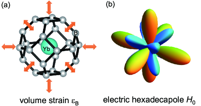
Figure 1: Schematic view of the volume strain and the hexadecapole in YbB₁₂. (a) Crystal lattice around the Yb ion Kanai_JPSJ84 and volume strain $\varepsilon_{\mathrm{B}}$ with the irrep $\Gamma_{1}$ of $O_{h}$. Orange arrows indicate the isotropic deformation of the lattice. (b) Hexadecapole $H_{0}$ with $\Gamma_{1}$ symmetry obtained as a result of an isotropic change of the Yb ionic radius.

As shown in previous reports Tamaki_JPhysC18 ; Nemoto_PRB61 ; Goto_PRB59 , ultrasonic measurements are a powerful tool to detect valence fluctuations. In particular, in the Kondo insulator SmB₆, the decrease in the bulk modulus $C_{\mathrm{B}}$ with decreasing temperatures, namely the elastic softening of $C_{\mathrm{B}}$, has been revealed as a result of valence fluctuations between Sm²⁺ and Sm³⁺ Nakamura_JPSJ60_SmB6 . The relation between the energy gap of $c$-$f$ hybridized bands and the elastic softening is also discussed in terms of the interaction between $4f$ electrons and the bulk strain $\varepsilon_{\mathrm{B}}$ with full symmetry $\Gamma_{1}$. Several theoretical studies have proposed such a contribution of the $c$-$f$ hybridization to the elasticity Luthi_JMMM63 ; Thalmeier_JPhysC20 ; Keller_PRB41 ; Rout_PhysicaB367 . Therefore, we measured relevant elastic constants in zero and high fields searching for an elastic softening related to the valence fluctuations in YbB₁₂.

This paper is organized as follows. In Sec. II, experimental details of sample preparation and ultrasonic measurements in pulsed magnetic fields are explained. In Sec. III, we present the results of our ultrasonic experiments of YbB₁₂. In zero field, an increase in the elastic constants with decreasing temperatures, namely elastic hardening, accompanying curvature changes reveals some contribution of valence fluctuations to the elasticity. In contrast to zero field, a field-induced softening of the bulk modulus $C_{\mathrm{B}}$ appears, which indicates field-induced valence fluctuations due to $c$-$f$ hybridization. In Sec. IV, we analyzed the measured elastic constants using a multipole-susceptibility model. The field-induced valence fluctuations can be described in terms of the hexadecapole-volume strain coupling. Our analysis also confirms the decrease of the energy gap in high fields. We summarize our results in Sec. V.

II Experiment

Single crystals of YbB₁₂ were grown using the floating-zone method Iga_JMMM177 . Laue x-ray backscattering was used to align, cut, and polish samples with (110), (1$\bar{1}$0), ($\bar{1}$10), ($\bar{1}$$\bar{1}$0), (001), and (00$\bar{1}$) faces and the size of $1.033$ mm $\times 1.030$ mm $\times 3.763$ mm. An ultrasound pulse-echo method with a numerical vector-type phase-detection technique was used to measure the ultrasound velocity $v$ Fujita_JPSJ80 . The elastic constant $C=\rho v^{2}$ was determined from $v$ and the calculated mass density $\rho=4.828$ g/cm³ using the lattice constant $a=7.469\mathrm{\AA}$ Kasaya_JMMM31 . Piezoelectric transducers using LiNbO₃ plates with a 36^∘ Y-cut and 41^∘ X-cut (YAMAJU CERAMICS CO.) were employed to generate longitudinal ultrasonic waves with the fundamental frequency of approximately $f$ = 30 MHz and transverse waves with 18 MHz, respectively. As indicated in Fig. 2, higher-harmonic frequencies were used to obtain high-resolution data. A room temperature vulcanizing rubber (Shin-Etsu Silicone KE-42T) was used to glue the LiNbO₃ on the sample. The direction of ultrasonic propagation, $\bm{q}$, and the direction of polarization, $\bm{\xi}$, for the elastic constant $C_{ij}$ are indicated in Fig. 2. Two nondestructive pulsed magnets were used: one with a pulse duration of 36 ms installed at the Institute for Solid State Physics, the University of Tokyo using a ⁴He cryostat, and another magnet with a pulse duration of 150 ms at the HLD-EMFL in Dresden using a ³He cryostat.

III Results

III.1 Temperature dependence of elastic constants

To gain more information on the Yb valence in YbB₁₂, we investigated the three elastic constants $C_{11}$, $C_{44}$, and $C_{\mathrm{T}}=\left(C_{11}-C_{12}\right)/2$. Their relations to the symmetry strain and electric multipole are summarized in Table 1 Inui_group ; Luthi Phys. Ac. . Figure 2 shows the temperature dependence of the elastic constants in zero field. We observed the elastic hardening of $C_{11}$, $C_{44}$, and $C_{\mathrm{T}}$ with lowering temperatures. We also observed the elastic hardening of $C_{11}$ from 300 K (see Appendix A). All elastic constants exhibit an additional hardening and a characteristic curvature change in the vicinity of $T^{\star}=35$ K. As shown by the solid curves in Fig. 2, the elastic constants would exhibit a monotonic increase with decreasing temperature Vershni_PRB2 if we do not consider multipole contributions, described in the following Sec. IV Luthi Phys. Ac. . Therefore, the additional features in the elastic constants of YbB₁₂ indicate the multipole contribution to elasticity.

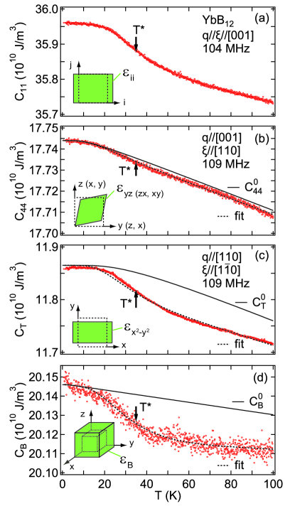
Figure 2: Temperature dependence of (a) the longitudinal elastic constant $C_{11}$, the transverse elastic constants (b) $C_{44}$ and (c) $C_{\mathrm{T}}=\left(C_{11}-C_{12}\right)/2$, and (d) the bulk modulus $C_{\mathrm{B}}$ calculated from $C_{11}$ and $C_{\mathrm{T}}$. The dotted lines indicate the fit of $C_{44}$, $C_{\mathrm{T}}$, and $C_{\mathrm{B}}$ in the framework of the phenomenological two-band model discussed in Sec. IV. The solid lines indicate the temperature dependence of the elastic constants without multipole contribution. The strains $\varepsilon_{\mathrm{ij}}$ for $C_{11}$, $C_{44}$, $C_{\mathrm{T}}$, and $C_{\mathrm{B}}$ are schematically shown in the inset in each panel. The vertical arrows in each panel indicate the characteristic temperature $T^{\star}$ discussed in Sec. IV.

To describe the origin of the anomaly in each elastic constant of YbB₁₂, we focus on the multipole effect of the CEF wave functions of localized $4f$ electrons taken into account the presence of $\Gamma_{8}$, $\Gamma_{7}$, and $\Gamma_{6}$ states Nemkovski_PRL99 ; Kanai_JPSJ84 . Since the direct product of the $\Gamma_{8}$ quartet is reduced as $\Gamma_{8}\otimes\Gamma_{8}=\Gamma_{1}\oplus\Gamma_{2}\oplus\Gamma_{3}\oplus 2\Gamma_{4}\oplus 2\Gamma_{5}$ Inui_group ; Kuramoto_JPSJ78 , we deduce that the $\Gamma_{8}$ ground-state wave functions carry the electric quadrupoles $O_{u}$ and $O_{v}$ with irrep $\Gamma_{3}$ and $O_{yz}$, $O_{zx}$, and $O_{xy}$ with irrep $\Gamma_{5}$ as summarized in Table 1. In addition, the $\Gamma_{8}$ quartet also provides the electric hexadecapole $H_{0}=O_{4}^{0}+5O_{4}^{4}$ with irrep $\Gamma_{1}$. Because the magnetic multipole degrees of freedom do not couple with the strain, we ignore magnetic dipoles with irrep $\Gamma_{4}$ and magnetic octupoles with irreps $\Gamma_{2}$, $\Gamma_{4}$, and $\Gamma_{5}$. This group-theoretical consideration indicates that the elastic softening of $\left(C_{11}-C_{12}\right)/2$ with irrep $\Gamma_{3}$ and $C_{44}$ with irrep $\Gamma_{5}$ is due to a multipole-strain interaction described as

$$H_{\mathrm{MS}}=-g_{\Gamma_{\gamma}}O_{\Gamma_{\gamma}}\varepsilon_{\Gamma_{\gamma}}.$$ (2)

Here, $g_{\Gamma_{\gamma}}$ is a coupling constant and $\Gamma_{\gamma}$ denotes the irrep. We show how to calculate the multipole susceptibility based on the CEF wave functions in Appendix B. Because the calculated multipole susceptibility for $\Gamma_{3}$- and $\Gamma_{5}$-type quadrupoles shows a divergent increase for decreasing temperatures, a divergent elastic softening is theoretically expected in $C_{44}$ and $C_{\mathrm{T}}$. However, our experimental results show no softening in all measured elastic constants. Therefore, the CEF approach based on a localized $4f$ character does not apply to the elasticity of YbB₁₂ in zero field.

The other possible scenario describing the additional contribution around $T^{\star}$ is a result of the charge freezing of Yb without long-range ordering as previously discussed in the samarium compounds Sm₃Se₄ and Sm₃Te₄ Tamaki_JPhysC18 ; Nemoto_PRB61 . Since the charge freezing would be characterized by a frequency-dependent ultrasound response, we measured the elastic constants and ultrasonic attenuation coefficients for several frequencies. However, we did not observe any frequency dependence neither in the elastic constants nor in the ultrasonic attenuation coefficients between 30 and 160 MHz.

Table 1: Symmetry strains, electric multipoles, and elastic constants corresponding to the irreducible representations (irreps) of the space group $O_{h}$.

Irrep	Symmetry strain	Electric multipole	Elastic constant
$\Gamma_{1}$	$\varepsilon_{\mathrm{B}}=\varepsilon_{xx}+\varepsilon_{yy}+\varepsilon_{zz}$	$O_{4}^{0}+5O_{4}^{4}(=H_{0})$	$C_{\mathrm{B}}=\left(C_{11}+2C_{12}\right)/3$
$\Gamma_{3}$	$\varepsilon_{u}=(2\varepsilon_{zz}-\varepsilon_{xx}-\varepsilon_{yy})/\sqrt{3}$	$O_{u(=3z^{2}-r^{2})}$	$C_{\mathrm{T}}=\left(C_{11}-C_{12}\right)/2$
	$\varepsilon_{v}=\varepsilon_{xx}-\varepsilon_{yy}$	$O_{v(=x^{2}-y^{2})}$
$\Gamma_{5}$	$\varepsilon_{yz}$	$O_{yz}$	$C_{44}$
	$\varepsilon_{zx}$	$O_{zx}$
	$\varepsilon_{xy}$	$O_{xy}$

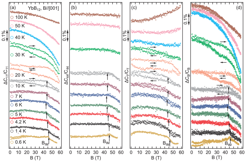
Figure 3: Magnetic-field dependence of the relative variation of the elastic constants $\Delta C_{ij}/C_{ij}=\left[C_{ij}(B)-C_{ij}(B=0)\right]/C_{ij}(B=0)$ at several temperatures for $B\|[001]$. Field dependence of (a) the longitudinal elastic constant $C_{11}$, the transverse elastic constants (b) $C_{44}$ and (c) $C_{\mathrm{T}}$, and (d) the bulk modulus $C_{\mathrm{B}}$. The data sets are shifted consecutively along the $\Delta C/C$ axes for clarity. The vertical arrows indicate the insulator-metal transition field $B_{\mathrm{IM}}$. The horizontal arrows show the field-sweep directions.

Therefore, we focus on the contribution of valence fluctuations to the elasticity caused by the $c$-$f$ hybridization. Figure 2(d) shows the temperature dependence of the bulk modulus $C_{\mathrm{B}}=(C_{11}+2C_{12})/3=C_{11}-4C_{\mathrm{T}}/3$ with the irrep $\Gamma_{1}$ calculated from the experimental results of $C_{11}$ and $C_{\mathrm{T}}$. $C_{\mathrm{B}}$ exhibits as well a hardening with an additional contribution in the vicinity of 35 K. This result for YbB₁₂ is in contrast to the significant softening of $C_{\mathrm{B}}$ due to Sm valence fluctuations observed in SmB₆. In Sec. IV, we will discuss the origin of the additional contribution in terms of the multipole susceptibility based on a two-band model to confirm the contribution of valence fluctuations to the elastic constants in zero field.

III.2 Magnetic-field dependence of elastic constants

To investigate the valence properties of YbB₁₂ in magnetic fields, we measured the elastic constants $C_{11}$, $C_{44}$, and $C_{\mathrm{T}}$ up to 59 T for $B\|[001]$. Figure 3 shows the magnetic-field dependence of the relative variation of the elastic constants $\Delta C_{ij}/C_{ij}$ at several temperatures. We observed a field-induced IM transition and elastic softening for each elastic constant in the Kondo-metal phase. Below 10 K, this softening appears rather abruptly above the insulator-metal transition field $B_{\mathrm{IM}}$. $B_{\mathrm{IM}}$ are comparable with results of a previous magnetocaloric-effect study Terashima_PRL120 . Since $C_{\mathrm{B}}$ contains $C_{11}$ and $C_{\mathrm{T}}$, our experimental results show as well the softening of $C_{\mathrm{B}}$ in the Kondo-metal phase.

Above 10 K, no sharp anomaly corresponding to the Kondo-metal phase transition is visible any more. However, $C_{11}$ still shows a significant softening in magnetic field contrary to the other elastic constants (Fig. 3). In particular, at 40 K, $C_{11}$ exhibits a large softening of $0.30\%$ at 59 T while $C_{\mathrm{T}}$ shows a softening of only $0.027\%$. The softening of $C_{11}$ at 100 K is also in contrast to the hardening observed for $C_{\mathrm{T}}$.

Between 10 and 30 K, a clear hysteresis appears in the pulsed-field data of $C_{11}$ and $C_{\mathrm{T}}$ (Fig. 3). This is approximately the temperature range where the additional contribution to the elastic constants is detected (Fig 2). As shown in a previous magnetocaloric-effect study in adiabatic condition below 7 K Terashima_PRL120 , the temperature of the sample is reduced by the application of a magnetic field. Because of the quasi-adiabatic experimental conditions, the final temperature after the field pulse fields might be higher than assumed which may cause the hysteresis. Therefore, the hysteresis of elastic constants $C_{11}$ and $C_{\mathrm{T}}$ can also be attributed to the magnetocaloric effect.

We also looked for the quantum oscillation in YbB₁₂ Xiang_Science362 . In principle, such quantum oscillations may appear as well in bulk sensitive ultrasound properties. However, we were not able to resolve any acoustic de Haas-van Alphen effect at least 0.6 K. This result may imply a weak electron-phonon interaction for the studied acoustic modes.

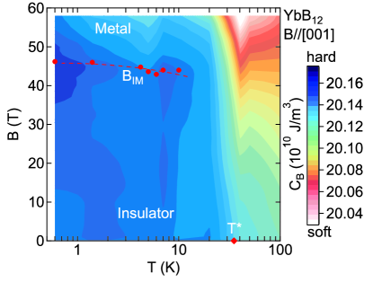
Figure 4: Temperature-field phase diagram of YbB₁₂ for $B\|[001]$. The filled red circles indicate the insulator-metal transition field $B_{\mathrm{IM}}$. The filled red diamond indicates the characteristic temperature $T^{\star}$ (see text for details). The color code shows the value of the bulk modulus $C_{\mathrm{B}}$.

We calculated $C_{\mathrm{B}}=C_{11}-4C_{\mathrm{T}}/3$ from the measured magnetic-field dependence of $C_{11}$ and $C_{\mathrm{T}}$ (Fig. 3). Indeed, $C_{\mathrm{B}}$ shows a very similar behavior as the individual elastic constants with a clear anomaly at $B_{\mathrm{IM}}$ below 10 K and hysteresis between 10 and 30 K. $B_{\mathrm{IM}}$ determined by our ultrasonic measurements are shown in Fig. 4.

$C_{\mathrm{B}}$ exhibits a small softening below 50 T at 20 K and 45 T at 30 K. By contrast, above 40 K, $C_{\mathrm{B}}$ shows monotonic softening with increasing fields. In particular, the largest softening of 0.52% is observed in $C_{\mathrm{B}}$ at 40 K. The field-induced elastic softening of $C_{\mathrm{B}}$ is summarized in the contour plot in Fig. 4.

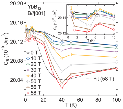
Figure 5: Temperature dependence of the bulk modulus $C_{\mathrm{B}}$ of YbB₁₂ at various magnetic fields for $B\|[001]$ extracted from the up-sweep data shown in Fig. 3, except for the zero-field data. The dotted line indicates the fit describing $C_{\mathrm{B}}$ in the framework of the phenomenological two-band model. The inset shows $C_{\mathrm{B}}$ below 10 K.

For further understanding of the field-induced elastic softening in YbB₁₂, we plotted the temperature dependence of $C_{\mathrm{B}}$ for various magnetic fields (Fig. 5). As shown in the inset of Fig. 5, $C_{\mathrm{B}}$ exhibits a softening of about $0.05\%$ below 7 K down to $\sim$ 2 K in magnetic fields above 40 T. In addition, $C_{\mathrm{B}}$ shows significant softening from 100 K down to 40 K in high fields, which is in contrast to the hardening of $C_{\mathrm{B}}$ in zero field. The softening of $C_{\mathrm{B}}$ is similar to that found for SmB₆ caused by $c$-$f$ hybridization-driven valence fluctuations corresponding to hexadecapole-strain interaction Nakamura_JPSJ60_SmB6 .

The experimental results of the temperature dependence and the magnetic field dependence of $C_{\mathrm{B}}$ of YbB₁₂ cannot be described by the localized $4f$-electron model (see Appendix C). In the following Sec. IV, therefore, we discuss our observations in terms of multipole-strain interaction and the multipole susceptibility for a two-band model.

IV Discussion

We discuss the origin of the elastic anomalies of YbB₁₂ in terms of a two-band model assuming a constant density of states (DOS) with respect to energy. This model has successfully reproduced the elastic softening observed in the Kondo compounds SmB₆ and CeNiSn Nakamura_JPSJ60_SmB6 ; Nakamura_JPSJ60_CeNiSn . In YbB₁₂, this phenomenological model also gives qualitative explanation for the temperature dependence of $C_{44}$, $C_{\mathrm{T}}$, and $C_{\mathrm{B}}$ in zero field and for $C_{\mathrm{B}}$ in high fields. Field-induced valence fluctuations are included by the hexadecapole-strain interaction. By that, the essential parameters for the explanation of our experimental results are identified (Table 2).

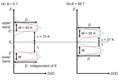
Figure 6: Schematic view of the two-band model assuming a constant DOS over each band (red rectangular). (a) DOS at zero field with an energy gap $2\Delta=140$ K and bandwidth $W=55$ K. (b) DOS at 58 T. The energy gap $2\Delta=74$ K and the bandwidth $W=55$ K is determined using Eq. (IV). The blue dotted curves indicate the schematic view of a more realistic DOS of YbB₁₂.

We introduce a two-band model, which is schematically shown in Fig. 6. In this model, we deal with the two $c$-$f$ hybridized bands: an upper band above the Fermi energy $E_{\mathrm{F}}$ with an energy $E_{0,\bm{k}}^{\mathrm{u}}$ and a lower band below $E_{\mathrm{F}}$ with $E_{0,\bm{k}}^{\mathrm{l}}$. The DOS with energy dispersion of each band is simplified to the rectangular form. The bandwidth $W$, the DOS $D$, and the band gap $2\Delta$ are set as shown in Fig. 6. We assume that the multipole-strain interaction for the electrons in the two bands can be written as Kurihara_JPSJ86

$$H_{\mathrm{MS}}=-\sum_{\bm{k}}\begin{pmatrix}c_{\bm{k},\mathrm{u}}^{\dagger}\cr c_{\bm{k},\mathrm{l}}^{\dagger}\end{pmatrix}^{T}\begin{pmatrix}&d_{\bm{k},\Gamma_{\gamma}}^{\mathrm{u}}&h_{\bm{k},\Gamma_{\gamma}}\cr&h_{\bm{k},\Gamma_{\gamma}}^{\ast}&d_{\bm{k},\Gamma_{\gamma}}^{\mathrm{l}}\end{pmatrix}\begin{pmatrix}c_{\bm{k},\mathrm{u}}\cr c_{\bm{k},\mathrm{l}}\end{pmatrix}\varepsilon_{\Gamma_{\gamma}}.$$ (3)

For the multipole-strain interaction $H_{\mathrm{MS}}$ of Eq. (2), the diagonal term $d_{\bm{k},\Gamma_{\gamma}}^{\mathrm{l(u)}}$ for the electrons in band $\mathrm{u(l)}$ indicates a renormalized multipole-strain coupling constant described as $g_{\mathrm{\Gamma_{\gamma}}}\langle\mathrm{u(l)}|O_{\mathrm{\Gamma_{\gamma}}}|\mathrm{u(l)}\rangle$. The off-diagonal term $h_{\bm{k},\Gamma_{\gamma}}$ is written as $g_{\mathrm{\Gamma_{\gamma}}}\langle\mathrm{u(l)}|O_{\mathrm{\Gamma_{\gamma}}}|\mathrm{l(u)}\rangle$. $c_{\bm{k},\mathrm{u(l)}}$ and $c_{\bm{k},\mathrm{u(l)}}^{\dagger}$ are annihilation and creation operators of an electron in the band $\mathrm{u(l)}$ with wave vector $\bm{k}$, respectively. Considering the Anderson Hamiltonian describing $c$-$f$ hybridization, we deduce that the multipole-strain interaction of Eq. (3) originates from electron-phonon interaction consisting of $c$-$f$ and $f$-$f$ terms Rout_PhysicaB367 . The multipole-strain interaction of Eq. (3) for the two-band model provides a second-order perturbation for the upper band, the lower one, and the band gap. The perturbation energies of each band and the perturbation energy gap are described as Nakamura_JPSJ60_SmB6 ; Nakamura_JPSJ60_CeNiSn

$$E_{\bm{k}}^{\mathrm{u}}\left(\varepsilon_{\Gamma_{\gamma}}\right)=E_{0,\bm{k}}^{\mathrm{u}}-d_{\bm{k},\Gamma_{\gamma}}^{\mathrm{u}}\varepsilon_{\Gamma_{\gamma}}+\frac{\left|h_{\bm{k},\Gamma_{\gamma}}\right|^{2}}{2\Delta_{\bm{k}}}\varepsilon_{\Gamma_{\gamma}}^{2},$$ (4)

$$E_{\bm{k}}^{\mathrm{l}}\left(\varepsilon_{\Gamma_{\gamma}}\right)=E_{0,\bm{k}}^{\mathrm{l}}-d_{\bm{k},\Gamma_{\gamma}}^{\mathrm{l}}\varepsilon_{\Gamma_{\gamma}}-\frac{\left|h_{\bm{k},\Gamma_{\gamma}}\right|^{2}}{2\Delta_{\bm{k}}}\varepsilon_{\Gamma_{\gamma}}^{2},$$ (5)

$$\Delta_{\bm{k}}\left(\varepsilon_{\Gamma_{\gamma}}\right)=\Delta_{\bm{k}}-\frac{1}{2}\left(d_{\bm{k},\Gamma_{\gamma}}^{\mathrm{u}}-d_{\bm{k},\Gamma_{\gamma}}^{\mathrm{l}}\right)\varepsilon_{\Gamma_{\gamma}}+\frac{\left|h_{\bm{k},\Gamma_{\gamma}}\right|^{2}}{2\Delta_{\bm{k}}}\varepsilon_{\Gamma_{\gamma}}^{2}.$$ (6)

Here, $2\Delta_{\bm{k}}=E_{0,\bm{k}}^{\mathrm{u}}-E_{0,\bm{k}}^{\mathrm{l}}$ is the energy gap between the upper band and the lower one. The total free energy $F$ is written as Luthi_JMMM52

$$F =\frac{1}{2}C_{\Gamma_{\gamma}}^{0}\varepsilon_{\Gamma_{\gamma}}^{2}+nE_{\mathrm{F}}\left(\varepsilon_{\Gamma_{\gamma}}\right)$$

$$-k_{\mathrm{B}}T\sum_{s(=\mathrm{u,l}),\bm{k}}\ln\left\{1+\exp\left[{-\frac{E_{\bm{k}}^{s}\left(\varepsilon_{\Gamma_{\gamma}}\right)-E_{\mathrm{F}}\left(\varepsilon_{\Gamma_{\gamma}}\right)}{k_{\mathrm{B}}T}}\right]\right\}.$$ (7)

Here, $C_{\Gamma_{\gamma}}^{0}$ is the elastic constant due to the phonon part with the irrep $\Gamma_{\gamma}$, $n$ is the total number of conduction electrons, $E_{\mathrm{F}}(\varepsilon_{\Gamma_{\gamma}})$ is the Fermi energy in the deformed system, and $k_{\mathrm{B}}$ is the Boltzmann constant. The first term on the right-hand side of Eq. (IV) corresponds to the lattice part. The second and third terms correspond to the free energy of the conduction electrons. The second derivative of the total free energy with respect to the strain $\varepsilon_{\Gamma}$ provides the elastic constant $C_{\Gamma_{\gamma}}(T)$ described as

$$C_{\Gamma_{\gamma}}(T) =C_{\Gamma_{\gamma}}^{0}+\sum_{s,\bm{k}}\frac{\partial^{2}E_{\bm{k}}^{s}}{\partial\varepsilon_{\Gamma_{\gamma}}^{2}}f_{\bm{k}}^{s}$$

$$-\frac{1}{k_{\mathrm{B}}T}\sum_{s,\bm{k}}\left(\frac{\partial E_{\bm{k}}^{s}}{\partial\varepsilon_{\Gamma_{\gamma}}}\right)^{2}f_{\bm{k}}^{s}\left(1-f_{\bm{k}}^{s}\right)$$

$$+\frac{1}{k_{\mathrm{B}}T}\frac{\sum_{s,\bm{k}}\left[\frac{\partial E_{\bm{k}}^{s}}{\partial\varepsilon_{\Gamma_{\gamma}}}f_{\bm{k}}^{s}\left(1-f_{\bm{k}}^{s}\right)\right]^{2}}{\sum_{s,\bm{k}}f_{\bm{k}}^{s}\left(1-f_{\bm{k}}^{s}\right)}.$$ (8)

Here, $f_{\bm{k}}^{s}=\{1+\exp[(E_{0,\bm{k}}^{s}-E_{\mathrm{F}})/k_{\mathrm{B}}T]\}^{-1}$ is the Fermi distribution function. $\partial E_{\bm{k}}^{s}\left(\varepsilon_{\Gamma_{\gamma}}\right)/\partial\varepsilon_{\Gamma_{\gamma}}|_{\varepsilon_{\Gamma_{\gamma}}\rightarrow 0}$ and $\partial^{2}E_{\bm{k}}^{s}\left(\varepsilon_{\Gamma_{\gamma}}\right)/\partial\varepsilon_{\Gamma_{\gamma}}^{2}|_{\varepsilon_{\Gamma_{\gamma}}\rightarrow 0}$ are written as $\partial E_{\bm{k}}^{s}/\partial\varepsilon_{\Gamma_{\gamma}}$ and $\partial^{2}E_{\bm{k}}^{s}/\partial\varepsilon_{\Gamma_{\gamma}}^{2}$ , respectively. The conservation law for the total electron number with respect to the strain, $\partial n/\partial\varepsilon_{\Gamma_{\gamma}}=\sum_{\bm{k}}\partial f_{\bm{k}}/\partial\varepsilon_{\Gamma_{\gamma}}=0$, is employed to calculate Eq. (IV). The second term on the right-hand side of Eq. (IV) corresponds to van Vleck term, which originates from the off-diagonal element $h_{\bm{k},\Gamma_{\gamma}}$ in the multipole-strain interaction of Eq. (3). The third and fourth terms are the Curie terms $(\sim 1/T)$ related to the diagonal elements $d_{\bm{k},\Gamma_{\gamma}}^{\mathrm{l}}$ and $d_{\bm{k},\Gamma_{\gamma}}^{\mathrm{u}}$. In this two-band model, the matrix elements of a multipole and the band gap are independent on the wave vector $\bm{k}$. The temperature dependence of the elastic constant is obtained by replacing the sum over the wave vector $\sum_{\bm{k}}$ by the energy integral using the DOS of the two-band model shown in Fig. 6 as Nakamura_JMMM76 ,

$$C_{\Gamma_{\gamma}}\left(T\right)=C_{\Gamma_{\gamma}}^{0}$$

$$-\frac{1}{4}D\left(d_{\Gamma_{\gamma}}^{\mathrm{u}}-d_{\Gamma_{\gamma}}^{\mathrm{l}}\right)^{2}\left[\tanh\left(\frac{\Delta+W}{2k_{\mathrm{B}}T}\right)-\tanh\left(\frac{\Delta}{2k_{\mathrm{B}}T}\right)\right]$$

$$+D\left|h_{\Gamma_{\gamma}}\right|^{2}\frac{2k_{\mathrm{B}}T}{\Delta}\ln\left|\frac{\cosh\left(\frac{\Delta}{2k_{\mathrm{B}}T}\right)}{\cosh\left(\frac{\Delta+W}{2k_{\mathrm{B}}T}\right)}\right|.$$ (9)

Here, we adopt the background elastic constant $C_{\Gamma_{\gamma}}^{0}=A-B/(e^{C/T}-1)$ Vershni_PRB2 . $C_{\Gamma_{\gamma}}^{0}$, $D(d_{\Gamma_{\gamma}}^{\mathrm{u}}-d_{\Gamma_{\gamma}}^{\mathrm{l}})^{2}$, and $D|h_{\Gamma_{\gamma}}|^{2}$ in Eq. (IV) are treated as fit parameters. The second and third terms in Eq. (IV) correspond to Curie and van Vleck term, respectively.

Table 2: Fit parameters determined by the analysis of the elastic constants $C_{44}$, $C_{\mathrm{T}}$, and $C_{\mathrm{B}}$ in zero field using the multipole susceptibility given in Eq. (IV). Parameters describing $C_{\mathrm{B}}$ at $58$ T are also listed. $D=2.25\times 10^{27}$ K^-1m^-3 in zero field is calculated from $|d_{\mathrm{B}}^{\mathrm{u}}-d_{\mathrm{B}}^{\mathrm{l}}|/k_{\mathrm{B}}$. $|d_{\mathrm{B}}^{\mathrm{u}}-d_{\mathrm{B}}^{\mathrm{l}}|/k_{\mathrm{B}}$ of $C_{\mathrm{B}}$ at 58 T is derived from the rigid-band approximation. The parameters for SmB₆ are reproduced from Ref. Nakamura_JPSJ60_SmB6 .

$C_{\Gamma_{\gamma}}$	$\Delta\left(\mathrm{K}\right)$	$W\left(\mathrm{K}\right)$	$D(d_{\Gamma_{\gamma}}^{\mathrm{u}}-d_{\Gamma_{\gamma}}^{\mathrm{l}})^{2}\left(10^{9}\mathrm{J}/\mathrm{m}^{3}\right)$	$A\left(10^{10}\mathrm{J}/\mathrm{m}^{3}\right)$	$B\left(\mathrm{J}/\mathrm{m}^{3}\right)$	$C\left(\mathrm{K}\right)$	$|d_{\Gamma_{\gamma}}^{\mathrm{u}}-d_{\Gamma_{\gamma}}^{\mathrm{l}}|/k_{\mathrm{B}}\left(\mathrm{K}\right)$
$C_{44}$	70	55	0.352	$17.744$	$1.25\times 10^{8}$	$32$	106
$C_{\mathrm{T}}$	70	55	8.58	$11.865$	$1.41\times 10^{9}$	$85$	526
$C_{\mathrm{B}}$ $(0\ \mathrm{T})$	70	55	3.30	$20.146$	$9.7\times 10^{6}$	$6$	326
$C_{\mathrm{B}}$ $(58\ \mathrm{T})$	37	55	10.3	$20.146$	$9.7\times 10^{6}$	$6$	(576)
$C_{\mathrm{B}}$ (SmB6)	160	150	25.6				1280

The analysis by the multipole susceptibility of Eq. (IV) reveals the contribution of valence fluctuations to the elastic constant in zero field. Fits to the temperature dependence of the elastic constants $C_{44}$, $C_{\mathrm{T}}$, and $C_{\mathrm{B}}$ in zero field are shown in Fig. 2. The fit parameters are summarized in Table 2. Here, we adopt $\Delta=70$ K and $W=55$ K at 0 T as determined by the analysis of specific-heat data of YbB₁₂ based on the rectangular two-band model Iga_JMMM177 . The temperature dependence of the elastic constants $C_{44}$, $C_{\mathrm{T}}$, and $C_{\mathrm{B}}$ can be well described by our model. The energy gap $\Delta$, the bandwidth $W$, and the coefficient of the Curie term, $D(d_{\Gamma_{\gamma}}^{\mathrm{u}}-d_{\Gamma_{\gamma}}^{\mathrm{l}})^{2}$, are necessary to reproduce the additional contribution in the vicinity of $T^{\star}=35$ K. In contrast, the van Vleck contribution is not needed to explain the experimental results. Our results indicate the importance of the multipole-strain interaction [Eq. (3)] to the elastic constants. In particular, the broad increase of $C_{\mathrm{B}}$ below $\sim$ 40 K seems to be the result of the isotropic change of the ionic radii caused by valence fluctuations due to the $c$-$f$ hybridization. We also tried to fit $C_{\mathrm{B}}$ to adopt $\Delta=30$ K as determined by the high-field magnetoresistance Sugiyama_JPSJ57 . However, we are not able to reproduce the curvature change in $C_{\mathrm{B}}$ around 35 K (see Appendix D).

The multipole susceptibility also provides the renormalized multipole-strain coupling constant and the interaction anisotropy. For the volume strain $\varepsilon_{\mathrm{B}}$, the first-order coefficient of the energy gap is described as $d\Delta(\varepsilon_{\mathrm{B}})/d\varepsilon_{\mathrm{B}}|_{\varepsilon_{\mathrm{B}}\rightarrow 0}=(d_{\mathrm{B}}^{\mathrm{u}}-d_{\mathrm{B}}^{\mathrm{l}})/2$ from Eq. (6). We can change the variable of this relation from $\varepsilon_{\mathrm{B}}$ to the hydrostatic pressure $P$, because $P=C_{\mathrm{B}}\varepsilon_{\mathrm{B}}$. In addition, we assume that $\Delta_{\bm{k}}$ in Eq. (6) corresponds to the activation energy $E$ determined by resistivity measurements. Thus, based on the hydrostatic pressure dependence of the resistivity of YbB₁₂ Iga_PhysB186 , we can estimate the renormalized hexadecapole-strain coupling constant $|d_{\mathrm{B}}^{\mathrm{u}}-d_{\mathrm{B}}^{\mathrm{l}}|/k_{\mathrm{B}}$ to be $326$ K by $dE/dP=-0.809$ K/GPa $=-8.09\times 10^{-10}$ $\mathrm{K}/(\mathrm{J}/\mathrm{m}^{3})$ for $C_{\mathrm{B}}=20.146\times 10^{10}$ J/m³ (Table 2). This assumption also provides the DOS in zero field to be $D=2.25\times 10^{27}$ K^-1 m^-3 from $D(d_{\mathrm{B}}^{\mathrm{u}}-d_{\mathrm{B}}^{\mathrm{l}})^{2}=3.30\times 10^{9}$ J/m³ in Table 2. Accordingly, the coupling constant for each elastic mode was calculated (Table 2). The coupling constant for $C_{44}$ is approximately 5 and 3 times smaller than the coupling constant for $C_{\mathrm{T}}$ and $C_{\mathrm{B}}$, respectively. Therefore, the dominant interaction is caused by the bulk strain with $\Gamma_{1}$ and the symmetry-breaking strain with $\Gamma_{3}$. This result is useful to elucidate the quantum states, which carry the multipole degrees of freedom.

While valence fluctuations are caused by hexadecapole-strain interactions in YbB₁₂, the contribution of the fluctuations to the elasticity is unexpectedly small in zero field. As shown in Fig. 2, $C_{\mathrm{B}}$ does not exhibit a softening in YbB₁₂. This result is quite different from the 3.8$\%$ softening in $C_{\mathrm{B}}$ observed for SmB₆. Furthermore, the coupling constant $|d_{\mathrm{B}}^{\mathrm{u}}-d_{\mathrm{B}}^{\mathrm{l}}|/k_{\mathrm{B}}=326$ K of YbB₁₂ is approximately 4 times smaller than $1280$ K reported for $C_{\mathrm{B}}$ of SmB₆ Nakamura_JPSJ60_SmB6 .

In contrast to zero field, strong valence fluctuations are revealed in applied magnetic fields. A fit to the temperature-dependent data of $C_{\mathrm{B}}$ at 58 T is shown in Fig. 5 (dashed line). The fit parameters at 58 T are also summarized in Table 2. In this analysis, we did not change $C_{\mathrm{B}}^{0}$ from that in zero field. We fixed the bandwidth $W=55$ K as the previously proposed rigid-band model Terashima_JPSJ86 , . The softening with the minimum at 40 K is reproduced qualitatively. Notably, the coefficient of the Curie term $D(d_{\mathrm{B}}^{\mathrm{u}}-d_{\mathrm{B}}^{\mathrm{l}})^{2}$ is enhanced from $3.30\times 10^{9}$ J/m³ at 0 T to $10.3\times 10^{9}$ J/m³ at 58 T. Thus, the quantum state contributing to the Curie term of YbB₁₂ might approach that of SmB₆ in magnetic fields. We stress that the hexadecapole-strain interaction originates from the coupling between the isotropic volume change of the crystal lattice and the change of ionic radii due to valence fluctuations. Therefore, the larger $D(d_{\mathrm{B}}^{\mathrm{u}}-d_{\mathrm{B}}^{\mathrm{l}})^{2}$ in magnetic fields indicates the enhancement of valence fluctuations of Yb.

A reduced energy gap is a plausible result of the IM transition. Our analysis reveals that the energy gap $2\Delta=140$ K at 0 T is reduced to 74 K at 58 T. This may be attributed to the Zeeman effect that changes the energy of the $4f$ states (see Appendix C). However, this two-band model cannot describe the gap closing in high fields. Since the DOS is approximated as constant, we cannot describe the IM transition due to the overlap of the edge of DOS at the Fermi energy as schematically illustrated in Fig. 6. An analysis using more realistic DOS as proposed in a previous study Ohashi_PRB70 ; Terashima_JPSJ86 is needed to describe the field-induced metal state in high fields.

Since the DOS in zero field is estimated by using the pressure dependence of the activation energy of YbB₁₂, we cannot apply $D$ to estimate the coupling constant $|d_{\mathrm{B}}^{\mathrm{u}}-d_{\mathrm{B}}^{\mathrm{l}}|/k_{\mathrm{B}}$ in high fields. Nevertheless, if we estimate the coupling constant assuming a field-independent rigid-band model with energy gap, the field-enhanced value of $576$ K can be obtained. The increase in the elastic softening due to the increase in the coupling constant is also consistent with a previous theoretical study of the electron-phonon coupling mediated by conduction electrons and $f$-electrons Rout_PhysicaB367 . Although the model needs to be improved, this interpretation seems to be plausible.

For further discussion of the field-enhanced valence fluctuations in YbB₁₂, we estimated the valence change of Yb in high fields. Previous studies on SmB₆ have revealed a valence change from $2.59\pm 0.01$ at 300 K to $2.53\pm 0.01$ at 60 K Mizumaki_JPhysConfSer176 and a softening of $C_{\mathrm{B}}$ by $3.1\%$ from 300 to 60 K Nakamura_JPSJ60_SmB6 . We assume that the valence change is proportional to the amount of elastic softening as a result of hexadecapole-strain interaction. Thus, the valence change is estimated to be -0.019 per 1$\%$ of elastic softening. Since the softening of $C_{\mathrm{B}}$ in SmB₆ and YbB₁₂ are described by the hexadecapole susceptibility based on the two-band model, we assume that the valence change per elastic softening applies to YbB₁₂ as well. Since the contribution of the hexadecapole-strain interaction to the elastic softening in YbB₁₂, namely the coefficient of the Curie term $D(d_{\mathrm{B}}^{\mathrm{u}}-d_{\mathrm{B}}^{\mathrm{l}})^{2}$, is $2.5$ times smaller than in SmB₆ (Table 2), the contribution of valence fluctuations to the elastic softening in YbB₁₂ is reduced by a factor of $2.5$. At 1.4 K, in the high-field Kondo-metal phase, the 0.09% softening from $B_{\mathrm{IM}}$ to 58 T (Fig. 3) indicates a small valence change of only approximately $-0.00069$. Furthermore, at 40 K, a valence change of approximately $-0.0040$ is estimated from the $0.52\%$ softening of $C_{\mathrm{B}}$. Such a valence change at 40 K may be detectable by high-field synchrotron x-ray measurements Matsuda_KPS62 .

Our results seem to be in conflict with the localized tendency of $4f$ states in the magnetic fields Aoki_PRL71 ; Matsuda_PRB86 ; Matsuda_SCES2013 . For a comprehensive understanding of the results, we discuss the Zeeman mixing and hybridization between Yb and B electrons in addition to the $c$-$f$ hybridization due to the $5d$ and $4f$ electrons of the Yb atoms. In YbB₁₂, the contribution of the $\Gamma_{6}$ and $\Gamma_{7}$ states to the ground state is enhanced by the Zeeman effect (see appendix C, Fig. 9). Thus, we expect that magnetic fields reduce the anisotropy of the electronic states due to the contributions of the $\Gamma_{8}$, $\Gamma_{6}$, and $\Gamma_{7}$ wave functions in YbB₁₂. In addition, as shown in Fig. 1(a), the Yb ion of YbB₁₂ is surrounded by a highly isotropic cage made up of 24 borons. This indicates an isotropic hybridization between the Yb $4f$ electrons and the B $2p$ electrons in addition to the $5d$-$4f$ hybridization. Thus, we suggest that the valence fluctuations are induced by the interatomic $p$-$f$ hybridization due to the isotropic wave function in high fields. Furthermore, a field-induced $p$-$f$ hybridization is consistent with the enhancement of the hexadecapole-strain interaction in high fields. In general, the matrix element of the hexadecapole $H_{0}$ for the wave function $\psi$ is given by $\int d\bm{r}\psi^{\ast}H_{0}\psi$. Therefore, a spatially expanded wave function, which is expected due to the interatomic type $p$-$f$ hybridization, might enhance the renormalized multipole-strain coupling $d_{\mathrm{B}}^{\mathrm{u(l)}}$ in Eq. (3). Our assumption is consistent with the isotropic resistivity in the low-temperature Kondo-metal phase Iga_JPhysConfSer200 . Although the crystal structure and magnetic character are different from those of YbB₁₂, the similar mechanisms of field-induced $p$-$f$ hybridization and delocalization of $4f$ electrons have been proposed in the heavy-fermion compound CeRhIn₅ to describe the emergence of an anisotropic electronic state in high fields Moll_NatComm6 ; Ronning_Nature548 ; Rosa_PRL122 ; Kurihara_PRB101 .

V Conclusion

In the present work, we investigated valence fluctuations of YbB₁₂ in zero and high fields by use of ultrasonic measurements. In zero field, the additional elastic hardening of $C_{11}$, $C_{44}$, $C_{\mathrm{T}}=\left(C_{11}-C_{12}\right)/2$, and the bulk modulus $C_{\mathrm{B}}=\left(C_{11}+2C_{12}\right)/3$ indicates only a small contribution of valence fluctuations to the elastic constants. In the Kondo-metal state, the valence fluctuations due to the $c$-$f$ hybridization are suggested to be enhanced by the field-induced elastic softening of $C_{\mathrm{B}}$. We found signatures of strong field-induced valence fluctuations in the vicinity of 40 K. Our phenomenological analysis of the temperature dependence of $C_{\mathrm{B}}$ based on the two-band model reveals that both, the additional contribution in zero field and the field-induced elastic softening, are reasonably described by the hexadecapole susceptibility. In particular, the field-induced elastic softening is attributed to the enhancement of the hexadecapole-strain coupling. This result indicates that the magnetic field enhances an isotropic volume change of the crystal lattice and the change of ionic radii due to valence fluctuations. Therefore, we propose field-induced valence fluctuations due to $c$-$f$ hybridization in YbB₁₂. In particular, we propose that the $p$-$f$ hybridization between Yb-$4f$ and B-$2p$ electrons plays a key role in high fields. The observed decrease of the energy gap in magnetic fields is explained by the energy shift of the $4f$ electrons due to the Zeeman effect.

Our study shows that ultrasonic measurements are useful to detect valence fluctuations. As suggested by a theoretical work Watanabe_JPSJ89 , such measurements may play a key role in the study of valence quantum criticality. We expect that field-induced valence fluctuations appear in other valence-fluctuating compounds.

Appendix A Temperature dependence of elastic constant $C_{11}$

Figure 7 shows the temperature dependence of the elastic constant $C_{11}$ in a wide temperature range of up to 300 K. $C_{11}$ exhibits an increase with decreasing temperatures from 300 K. This result indicates the elastic hardening of the bulk modulus $C_{\mathrm{B}}$ from 300 K down to low temperatures.

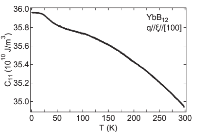
Figure 7: Temperature dependence of the longitudinal elastic constant $C_{11}$.

Appendix B Multipole susceptibility for CEF wave functions in zero field

Here, we present the CEF wave functions, the multipole matrices, and multipole susceptibility of YbB₁₂ assuming the localized $4f$ electrons. We show that the multipole susceptibility cannot describe our experimental results in Fig. 2.

To calculate the multipole susceptibility of YbB₁₂, we use CEF wave functions of the $4f$ electrons for Yb³⁺ with the total angular momentum $J=7/2$. The CEF Hamiltonian $H_{\mathrm{CEF}}$ under $O_{h}$ symmetry is written as

$$H_{\mathrm{CEF}}=B_{4}\left(O_{4}^{0}+5O_{4}^{4}\right)+B_{6}\left(O_{6}^{0}-21O_{6}^{4}\right).$$ (10)

Here, $B_{4}$ and $B_{6}$ are the CEF parameters. The matrix elements of $O_{4}^{0}$, $O_{4}^{4}$, $O_{6}^{0}$, and $O_{6}^{4}$ for $\left|J_{z}\right\rangle$ are listed in Ref. Hutchings . The wave functions diagonalizing $H_{\mathrm{CEF}}$ are given by Kanai_JPSJ84

$$\left|\Gamma_{8}^{1\pm}\right\rangle =-\sqrt{\frac{7}{12}}\left|\pm\frac{7}{2}\right\rangle+\sqrt{\frac{5}{12}}\left|\mp\frac{1}{2}\right\rangle,$$ (11)

$$\left|\Gamma_{8}^{2\pm}\right\rangle =\frac{1}{2}\left|\pm\frac{5}{2}\right\rangle+\frac{\sqrt{3}}{2}\left|\mp\frac{3}{2}\right\rangle,$$ (12)

$$\left|\Gamma_{6}^{1\pm}\right\rangle =\sqrt{\frac{5}{12}}\left|\pm\frac{7}{2}\right\rangle+\sqrt{\frac{7}{12}}\left|\mp\frac{1}{2}\right\rangle,$$ (13)

$$\left|\Gamma_{7}^{\pm}\right\rangle =-\frac{\sqrt{3}}{2}\left|\pm\frac{5}{2}\right\rangle+\frac{1}{2}\left|\mp\frac{3}{2}\right\rangle,$$ (14)

where $\left|\Gamma_{8}^{1\pm}\right>$ and $\left|\Gamma_{8}^{2\pm}\right>$ are the ground-state wave functions and $\left|\Gamma_{7}^{\pm}\right>$ and $\left|\Gamma_{6}^{\pm}\right>$ are the degenerate excited states. The matrix elements of $H_{\mathrm{CEF}}$ for the wave functions given in Eqs. (11) - (14) provide the eigenenergy of each CEF state described as $E_{\Gamma_{8}}=120\left(B_{4}+168B_{6}\right)$, $E_{\Gamma_{6}}=120\left(7B_{4}-210B_{6}\right)$, and $E_{\Gamma_{7}}=-120\left(9B_{4}+126B_{6}\right)$. The energy gap $\Delta_{\mathrm{CEF}}=23$ meV = $270$ K between the ground state and the excited states $\Gamma_{6}$ and $\Gamma_{7}$ Kanai_JPSJ84 provides the CEF parameters $B_{4}=-33.7$ meV and $B_{6}=-6.24$ meV.

The matrices of the hexadecapole $H_{0}=O_{4}^{0}+5O_{4}^{4}$ with irrep $\Gamma_{1}$, the quadrupoles $O_{u}$ and $O_{v}$ with $\Gamma_{3}$, and $O_{yz}$, $O_{zx}$, and $O_{xy}$ with $\Gamma_{5}$ for the wave functions (11) - (14) are calculated as

$$H_{0} =\bordermatrix{&\left|\Gamma_{8}^{1+}\right\rangle&\left|\Gamma_{8}^{1-}\right\rangle&\left|\Gamma_{8}^{2+}\right\rangle&\left|\Gamma_{8}^{2-}\right\rangle&\left|\Gamma_{6}^{+}\right\rangle&\left|\Gamma_{6}^{-}\right\rangle&\left|\Gamma_{7}^{+}\right\rangle&\left|\Gamma_{7}^{-}\right\rangle\cr&120&0&0&0&0&0&0&0\cr&0&120&0&0&0&0&0&0\cr&0&0&120&0&0&0&0&0\cr&0&0&0&120&0&0&0&0\cr&0&0&0&0&840&0&0&0\cr&0&0&0&0&0&840&0&0\cr&0&0&0&0&0&0&1080&0\cr&0&0&0&0&0&0&0&1080},$$ (15)

$$O_{u} =\begin{pmatrix}6&0&0&0&-3\sqrt{35}&0&0&0\cr 0&6&0&0&0&-3\sqrt{35}&0&0\cr 0&0&-6&0&0&0&-3\sqrt{3}&0\cr 0&0&0&-6&0&0&0&-3\sqrt{3}\cr-3\sqrt{35}&0&0&0&0&0&0&0\cr 0&-3\sqrt{35}&0&0&0&0&0&0\cr 0&0&-3\sqrt{3}&0&0&0&0&0\cr 0&0&0&-3\sqrt{3}&0&0&0&0\end{pmatrix},$$ (16)

$$O_{v} =\begin{pmatrix}0&0&0&\sqrt{105}&0&0&0&0\cr 0&0&2\sqrt{3}&0&0&0&-3&0\cr 0&2\sqrt{3}&0&0&0&\sqrt{105}&0&0\cr\sqrt{105}&0&0&0&2\sqrt{3}&0&0&0\cr 0&0&0&2\sqrt{3}&0&0&0&-3\cr 0&0&\sqrt{105}&0&0&0&0&0\cr 0&-3&0&0&0&0&0&0\cr 0&0&0&0&-3&0&0&0\end{pmatrix},$$ (17)

$$O_{yz} =\begin{pmatrix}0&0&0&0&0&0&\sqrt{35}i&0\cr 0&0&0&3\sqrt{3}i&0&0&0&-4i\cr 0&0&0&0&-3\sqrt{3}i&0&0&-2\sqrt{3}i\cr 0&-3\sqrt{3}i&0&0&0&0&-2\sqrt{3}i&0\cr 0&0&3\sqrt{3}i&0&0&0&-4i&0\cr 0&0&0&0&0&0&0&\sqrt{35}i\cr-\sqrt{35}i&0&0&2\sqrt{3}i&4i&0&0&0\cr 0&4i&2\sqrt{3}i&0&0&-\sqrt{35}i&0&0\end{pmatrix},$$ (18)

$$O_{zx} =\begin{pmatrix}0&0&0&0&0&0&-\sqrt{35}&0\cr 0&0&0&3\sqrt{3}&0&0&0&-4\cr 0&0&0&0&-3\sqrt{3}&0&0&4\sqrt{3}\cr 0&3\sqrt{3}&0&0&0&0&-4\sqrt{3}&0\cr 0&0&-3\sqrt{3}&0&0&0&4&0\cr 0&0&0&0&0&0&0&\sqrt{35}\cr-\sqrt{35}&0&0&-4\sqrt{3}&4&0&0&0\cr 0&-4&4\sqrt{3}&0&0&\sqrt{35}&0&0\end{pmatrix},$$ (19)

$$O_{xy} =\begin{pmatrix}0&0&0&0&0&0&0&-\sqrt{35}i\cr 0&0&3\sqrt{3}i&0&0&0&8i&0\cr 0&-3\sqrt{3}i&0&0&0&0&0&0\cr 0&0&0&0&3\sqrt{3}i&0&0&0\cr 0&0&0&-3\sqrt{3}i&0&0&0&-8i\cr 0&0&0&0&0&0&\sqrt{35}i&0\cr 0&-8i&0&0&0&-\sqrt{35}i&0&0\cr\sqrt{35}i&0&0&0&8i&0&0&0\end{pmatrix}.$$ (20)

Here, Stevens equivalent operators $O_{u}=3J_{z}^{2}-J\left(J+1\right)$, $O_{v}=J_{x}^{2}-J_{y}^{2}$, $O_{yz}=J_{y}J_{z}+J_{z}J_{y}$, $O_{zx}=J_{z}J_{x}+J_{x}J_{x}$, and $O_{xy}=J_{x}J_{y}+J_{y}J_{x}$, given by the components of the total angular momentum $J_{x}$, $J_{y}$, and $J_{z}$, are used to calculate the matrix elements. Considering the second-order perturbation processes for the $i$-th CEF state with energy $E_{i}^{0}$ due to the multipole-strain interaction of Eq. (2), which is described as

$$E_{i}\left(\varepsilon_{\Gamma_{\gamma}}\right)=E_{i}^{0} -g_{\Gamma_{\gamma}}\langle i\left|O_{\Gamma_{\gamma}}\right|i\rangle\varepsilon_{\Gamma_{\gamma}}$$

$$-g_{\Gamma_{\gamma}}^{2}\sum_{j\neq i}\frac{\left|\langle i\left|O_{\Gamma_{\gamma}}\right|j\rangle\right|^{2}}{E_{j}^{0}-E_{i}^{0}}\varepsilon_{\Gamma_{\gamma}}^{2},$$ (21)

the total free energy $F$, that consists of the CEF state and the strain, is written as

$$F\left(T,\varepsilon_{\Gamma_{\gamma}}\right)=\frac{1}{2}C_{\Gamma_{\gamma}}^{0}\varepsilon_{\Gamma_{\gamma}}^{2}-Nk_{\mathrm{B}}T\ln Z\left(\varepsilon_{\Gamma_{\gamma}}\right).$$ (22)

Here, $N$ is the number of Yb ions per unit volume and $Z(\varepsilon_{\Gamma_{\gamma}})$ is the partition function written as $Z(\varepsilon_{\Gamma_{\gamma}})=\sum_{i}\exp\left[-E_{i}(\varepsilon_{\Gamma_{\gamma}})/k_{\mathrm{B}}T\right]$. Thus, the elastic constant and the multipole susceptibility are calculated as

$$C_{\Gamma_{\gamma}}=\frac{\partial^{2}F}{\partial\varepsilon_{\Gamma_{\gamma}}^{2}}=C_{\Gamma_{\gamma}}^{0}-Ng_{\Gamma_{\gamma}}^{2}\chi_{\Gamma_{\gamma}},$$ (23)

$$-g_{\Gamma_{\gamma}}^{2}\chi_{\Gamma_{\gamma}}=\left\langle\frac{\partial^{2}E}{\partial\varepsilon_{\Gamma_{\gamma}}^{2}}\right\rangle$$

$$-\frac{1}{k_{\mathrm{B}}T}\left\{\left\langle\left(\frac{\partial E}{\partial\varepsilon_{\Gamma_{\gamma}}}\right)^{2}\right\rangle-\left\langle\frac{\partial E}{\partial\varepsilon_{\Gamma_{\gamma}}}\right\rangle^{2}\right\}.$$ (24)

Here, $C_{\Gamma_{\gamma}}^{0}$ is a background elastic constant, $\langle A\rangle$ is the thermal average using Boltzmann statistics written as $\langle A\rangle=\sum_{i}A_{i}\exp[-E_{i}/k_{\mathrm{B}}T]/Z$, and $\partial E(\varepsilon_{\Gamma_{\gamma}})/\partial\varepsilon_{\Gamma_{\gamma}}|_{\varepsilon_{\Gamma_{\gamma}}\rightarrow 0}$ and $\partial^{2}E(\varepsilon_{\Gamma_{\gamma}})/\partial\varepsilon_{\Gamma_{\gamma}}^{2}|_{\varepsilon_{\Gamma_{\gamma}}\rightarrow 0}$ are written as $\partial E/\partial\varepsilon_{\Gamma_{\gamma}}$ and $\partial^{2}E/\partial\varepsilon_{\Gamma_{\gamma}}^{2}$, respectively. The first term on the right-hand side of Eq. (B) corresponds to van Vleck term being constant at low temperatures and the second one to Curie term showing the reciprocal temperature dependence. The calculated multipole susceptibility $\chi_{\Gamma_{\gamma}}$ is shown in Fig. 8.

The hexadecapole susceptibility $\chi_{\mathrm{B}}$ would indicate a monotonic hardening of $C_{\mathrm{B}}$ below 100 K down to low temperatures because the temperature dependence of the elastic constant $C_{\mathrm{\Gamma_{\gamma}}}$ is given by $-\chi_{\mathrm{B}}$, i.e., the second term in Eq. (23). The divergent behavior of $\chi_{\Gamma_{3}}$ and $\chi_{\Gamma_{5}}$ would predict an elastic softening of $(C_{11}-C_{12})/2$ and $C_{44}$ at low temperatures, respectively. However, our experimental results of YbB₁₂ in zero field cannot be described by the susceptibility based on CEF wave functions using this picture, i.e., localized $4f$ electrons.

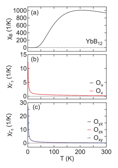
Figure 8: Temperature dependence of the electric multipole susceptibility of YbB₁₂. (a) Hexadecapole susceptibility $\chi_{\mathrm{B}}$ of $H_{0}=O_{4}^{0}+5O_{4}^{4}$ with $\Gamma_{1}$. This susceptibility provides the temperature dependence of the bulk modulus $C_{\mathrm{B}}$. (b) Quadrupole susceptibility $\chi_{\Gamma_{3}}$ of $O_{u}$ and $O_{v}$ with $\Gamma_{3}$ related to $(C_{11}-C_{12})/2$ (c) Quadrupole susceptibility $\chi_{\Gamma_{5}}$ of $O_{yz}$, $O_{zx}$, and $O_{xy}$ with $\Gamma_{5}$ related to $C_{44}$. As indicated in Eq. (23), $-\chi_{\Gamma_{\gamma}}$ contributes to these elastic constants. (The curves for $O_{u}$ and $O_{v}$ as well as for $O_{yz}$, $O_{zx}$, and $O_{xy}$ virtually lie on top of each other).

Appendix C Hexadecapole susceptibility for CEF wave functions in magnetic fields

In this section, the CEF wave functions, the hexadecapole matrix, and the hexadecapole susceptibility in magnetic fields of YbB₁₂ are presented assuming localized $4f$ electrons. We show that the elastic softening of $C_{\mathrm{B}}$ in high fields cannot be described by the hexadecapole susceptibility $\chi_{\mathrm{B}}$.

To calculate the hexadecapole susceptibility in magnetic fields, we consider the Zeeman Hamiltonian for $B\|[001]$ given by

$$H_{\mathrm{Zeeman}}=-g_{J}\mu_{\mathrm{B}}B_{0}J_{z}.$$ (25)

Here, $g_{J}$ is the Landé $g$-factor, $\mu_{\mathrm{B}}$ is the Bohr magneton, $B_{0}$ is the magnetic field, and $J_{z}$ is the magnetic dipole. Using the CEF wave functions of Eqs. (11)-(14), the matrix of $H_{\mathrm{Zeeman}}$ of Eq. (25) is written as

$$H_{\mathrm{Zeeman}} =\begin{pmatrix}-\frac{11}{6}B&0&0&0&\frac{\sqrt{35}}{3}B&0&0&0\cr 0&\frac{11}{6}B&0&0&0&-\frac{\sqrt{35}}{3}B&0&0\cr 0&0&\frac{1}{2}B&0&0&0&\sqrt{3}B&0\cr 0&0&0&-\frac{1}{2}B&0&0&0&-\sqrt{3}B\cr\frac{\sqrt{35}}{3}B&0&0&0&-\frac{7}{6}B&0&0&0\cr 0&-\frac{\sqrt{35}}{3}B&0&0&0&\frac{7}{6}B&0&0\cr 0&0&\sqrt{3}B&0&0&0&-\frac{3}{2}B&0\cr 0&0&0&-\sqrt{3}B&0&0&0&\frac{3}{2}B\end{pmatrix}.$$ (26)

Here, for the convenience, $B$ in the matrix elements of Eq. (26) is set as $B=g_{J}\mu_{\mathrm{B}}B_{0}$. The total Hamiltonian $H_{\mathrm{total}}=H_{\mathrm{CEF}}+H_{\mathrm{Zeeman}}$ is diagonalized as

$$H_{\mathrm{total}}=\bordermatrix{&\left|1+\right\rangle&\left|1-\right\rangle&\left|2+\right\rangle&\left|2-\right\rangle&\left|3+\right\rangle&\left|3-\right\rangle&\left|4+\right\rangle&\left|4-\right\rangle\cr&E_{1}^{+}&0&0&0&0&0&0&0\cr&0&E_{1}^{-}&0&0&0&0&0&0\cr&0&0&E_{2}^{+}&0&0&0&0&0\cr&0&0&0&E_{2}^{-}&0&0&0&0\cr&0&0&0&0&E_{3}^{+}&0&0&0\cr&0&0&0&0&0&E_{3}^{-}&0&0\cr&0&0&0&0&0&0&E_{4}^{+}&0\cr&0&0&0&0&0&0&0&E_{4}^{-}},$$ (27)

Here, the eigen energis in the matrix of Eq. (27) are written as

$$E_{1}^{\pm}=\frac{\Delta_{\mathrm{CEF}}-3B}{2}\pm\delta E_{1},$$ (28)

$$E_{2}^{\pm}=\frac{\Delta_{\mathrm{CEF}}+3B}{2}\pm\delta E_{2},$$ (29)

$$E_{3}^{\pm}=\frac{\Delta_{\mathrm{CEF}}-B}{2}\pm\delta E_{3},$$ (30)

$$E_{4}^{\pm}=\frac{\Delta_{\mathrm{CEF}}+B}{2}\pm\delta E_{4}.$$ (31)

For convenience, $\delta E_{i}$ in Eqs. (28) - (31) is set as

$$\delta E_{1}=\sqrt{\Delta E_{1}^{2}+\frac{35}{9}B^{2}},$$ (32)

$$\delta E_{2}=\sqrt{\Delta E_{2}^{2}+\frac{35}{9}B^{2}},$$ (33)

$$\delta E_{3}=\sqrt{\Delta E_{3}^{2}+3B^{2}},$$ (34)

$$\delta E_{4}=\sqrt{\Delta E_{4}^{2}+3B^{2}}.$$ (35)

We also set $\Delta E_{i}$ in Eqs. (32) - (35) as follows:

$$\Delta E_{1}=\frac{\Delta_{\mathrm{CEF}}}{2}+\frac{1}{3}B,$$ (36)

$$\Delta E_{2}=\frac{\Delta_{\mathrm{CEF}}}{2}-\frac{1}{3}B,$$ (37)

$$\Delta E_{3}=\frac{\Delta_{\mathrm{CEF}}}{2}-B,$$ (38)

$$\Delta E_{4}=\frac{\Delta_{\mathrm{CEF}}}{2}+B.$$ (39)

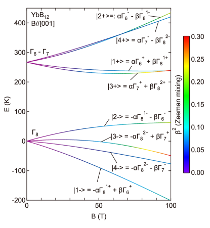
Figure 9: Magnetic-field dependence of the eigenenergy in $H_{\mathrm{total}}$ of Eq. (27) for $B\|[001]$. The color code shows the Zeeman mixing ratio $\beta_{i}^{2}$ in the wave functions of Eqs. (40)-(47).

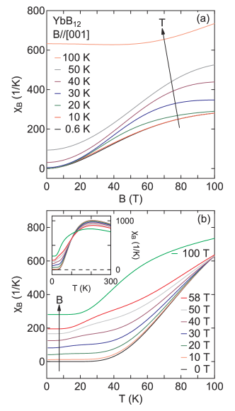
Figure 10: Electric hexadecapole susceptibility $\chi_{\mathrm{B}}$ of YbB₁₂ for $B\|[001]$. (a) Magnetic-field dependence of $\chi_{\mathrm{B}}$ at several temperatures. (b) Temperature dependence of $\chi_{\mathrm{B}}$ below 100 K in several magnetic fields. In the inset in (b), $\chi_{\mathrm{B}}$ is shown up to 300 K.

The wave functions diagonalizing the matrix Eq. (27) are written as

$$\left|1+\right\rangle=\alpha_{1}\left|\Gamma_{6}^{+}\right\rangle+\beta_{1}\left|\Gamma_{8}^{1+}\right\rangle,$$ (40)

$$\left|1-\right\rangle=\beta_{1}\left|\Gamma_{6}^{+}\right\rangle-\alpha_{1}\left|\Gamma_{8}^{1+}\right\rangle,$$ (41)

$$\left|2+\right\rangle=\alpha_{2}\left|\Gamma_{6}^{-}\right\rangle-\beta_{2}\left|\Gamma_{8}^{1-}\right\rangle,$$ (42)

$$\left|2-\right\rangle=-\beta_{2}\left|\Gamma_{6}^{-}\right\rangle-\alpha_{2}\left|\Gamma_{8}^{1-}\right\rangle,$$ (43)

$$\left|3+\right\rangle=\alpha_{3}\left|\Gamma_{7}^{+}\right\rangle+\beta_{3}\left|\Gamma_{8}^{2+}\right\rangle,$$ (44)

$$\left|3-\right\rangle=\beta_{3}\left|\Gamma_{7}^{+}\right\rangle-\alpha_{3}\left|\Gamma_{8}^{2+}\right\rangle,$$ (45)

$$\left|4+\right\rangle=\alpha_{4}\left|\Gamma_{7}^{-}\right\rangle-\beta_{4}\left|\Gamma_{8}^{2-}\right\rangle,$$ (46)

$$\left|4-\right\rangle=-\beta_{4}\left|\Gamma_{7}^{-}\right\rangle-\alpha_{4}\left|\Gamma_{8}^{2-}\right\rangle.$$ (47)

Here, the coefficients $\alpha_{i}$ and $\beta_{i}$ for $i=1,2,3,4$ in each wave function in Eqs. (40) - (47) are set as

$$\alpha_{1} =\frac{\Delta E_{1}+\delta E_{1}}{\sqrt{\left(\Delta E_{1}+\delta E_{1}\right)^{2}+\frac{35}{9}B^{2}}},$$ (48)

$$\alpha_{2} =\frac{\Delta E_{2}+\delta E_{2}}{\sqrt{\left(\Delta E_{2}+\delta E_{2}\right)^{2}+\frac{35}{9}B^{2}}},$$ (49)

$$\alpha_{3} =\frac{\Delta E_{3}+\delta E_{3}}{\sqrt{\left(\Delta E_{3}+\delta E_{3}\right)^{2}+3B^{2}}},$$ (50)

$$\alpha_{4} =\frac{\Delta E_{4}+\delta E_{4}}{\sqrt{\left(\Delta E_{4}+\delta E_{4}\right)^{2}+3B^{2}}},$$ (51)

$$\beta_{i} =\sqrt{1-\alpha_{i}^{2}}.$$ (52)

The magnetic-field dependence of the eigenenergies $E_{i}^{\pm}$ of Eqs. (28)-(31) are shown in Fig. 9. This result is consistent with the previous calculation for YbB₁₂ Terashima_JPSJ86 . The multipole susceptibility of Eq. (B) in magnetic field is calculated using the wave functions of Eqs. (40) - (47), the energy of Eqs. (28) - (31), the multipole matrices of Eqs. (15) - (20), the second-order perturbation of Eq. (B), and the free energy of Eq. (22).

In particular, we show the field-dependent hexadecapole susceptibility of $H_{0}$ in Fig. 10. Here, the matrix of the hexadecapole $H_{0}$ is written as

$$H_{0} =\bordermatrix{&\left|1+\right\rangle&\left|1-\right\rangle\cr&120\left(6\alpha_{1}^{2}+1\right)&720\alpha_{1}\beta_{1}\cr&720\alpha_{1}\beta_{1}&-120\left(6\alpha_{1}^{2}-7\right)}\oplus\bordermatrix{&\left|2+\right\rangle&\left|2-\right\rangle\cr&120\left(6\alpha_{2}^{2}+1\right)&-720\alpha_{2}\beta_{2}\cr&-720\alpha_{2}\beta_{2}&-120\left(6\alpha_{2}^{2}-7\right)}$$

$$\oplus\bordermatrix{&\left|3+\right\rangle&\left|3-\right\rangle\cr&-120\left(10\alpha_{3}^{2}-1\right)&-1200\alpha_{3}\beta_{3}\cr&-1200\alpha_{3}\beta_{3}&120\left(10\alpha_{3}^{2}-9\right)}\oplus\bordermatrix{&\left|4+\right\rangle&\left|4-\right\rangle\cr&-120\left(10\alpha_{4}^{2}-1\right)&-1200\alpha_{4}\beta_{4}\cr&-1200\alpha_{4}\beta_{4}&120\left(10\alpha_{4}^{2}-9\right)}.$$ (53)

The experimental results of the magnetic-field dependence of $C_{\mathrm{B}}$ at 20, 40, and 50 K (Fig. 3) can be qualitatively reproduced by the hexadecapole susceptibility $\chi_{\mathrm{B}}$ shown in Fig. 10(a). However, the experimental results of the elastic softening of $C_{\mathrm{B}}$ in high fields (Fig. 5) cannot be described by $\chi_{\mathrm{B}}$ shown in Fig. 10(b) since $\chi_{\mathrm{B}}$ indicates a hardening of $C_{\mathrm{B}}$ towards lower temperatures. Therefore, our experimental results of YbB₁₂ in high magnetic fields cannot be described by the susceptibility based on CEF wave functions of localized $4f$ electrons.

Appendix D Hexadecapole susceptibility for smaller energy gap

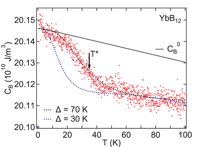
Figure 11: Fit of the bulk modulus $C_{\mathrm{B}}$ of YbB₁₂ by the hexadecapole susceptibility with energy gaps $\Delta=70$ and $30$ K.

Figure 11 shows the fit of bulk modulus $C_{\mathrm{B}}$ in YbB₁₂ by the hexadecapole susceptibility with energy gaps $\Delta=70$ K and $30$ K. We cannot describe the curvature change for $\Delta=30$ K, which corresponds to the activation energy determined by the high-field magnetoresistance Sugiyama_JPSJ57 . This result indicates that the contribution of the larger gap to the elasticity is dominant in zero field in YbB₁₂.

References

- (1) M. Kasaya, F. Iga, K. Negishi, S. Nakai, and T. Kasuya, J. Mag. Mag. Mat. 31-34, 437 (1983).
- (2) T. Susaki, A. Sekiyama, K. Kobayashi, T. Mizokawa, A. Fujimori, M. Tsunekawa, T. Muro, T. Matsushita, S. Suga, H. Ishii, T. Hanyu, A. Kimura, H. Namatame, M. Taniguchi, T. Miyahara, F. Iga, M. Kasaya, and H. Harima, Phys. Rev. Lett. 77, 4269 (1996).
- (3) K. S. Nemkovski, J.-M. Mignot, P. A. Alekseev, A. S. Ivanov, E. V. Nefeodova, A. V. Rybina, L.-P. Regnault, F. Iga, and T. Takabatake, Phys. Rev. Lett. 99, 137204 (2007).
- (4) Y. Kanai,T. Mori, S. Naimen, K. Yamagami, H. Fujiwara, A. Higashiya, T. Kadono, S. Imada, T. Kiss, A. Tanaka, K. Tamasaku, M. Yabashi, T. Ishikawa, F. Iga, and A. Sekiyama, J. Phys. Soc. Jpn. 84, 073705 (2015).
- (5) K. Ikushima, Y. Kato, M. Takigawa, F. Iga, S. Hiura, and T. Takabatake, Physica B 281-282, 274 (2000).
- (6) M. Kasaya, F. Iga, M. Takigawa, and T. Kasuya, J. Mag. Mag. Mat. 47 & 48, 429 (1985).
- (7) F. Iga, N. Shimizu, and T. Takabatake, J. Mag. Mag. Mat. 177-181, 337 (1998).
- (8) J. Yamaguchi, A. Sekiyama, S. Imada, H. Fujiwara, M. Yano, T. Miyamachi, G. Funabashi, M. Obara, A. Higashiya, K. Tamasaku, M. Yabashi, T. Ishikawa, F. Iga, T. Takabatake, and S. Suga, Phys. Rev. B 79, 125121 (2009).
- (9) T. Saso and H. Harima, J. Phys. Soc. Jpn. 72, 1131 (2003).
- (10) T. Ohashi, A. Koga, S. I. Suga, and N. Kawakami, Phys. Rev. B 70, 245104 (2004).
- (11) K. Sugiyama, F. Iga, M. Kasaya, T. Kasuya, and M. Date, J. Phys. Soc. Jpn. 57, 3946 (1988).
- (12) F. Iga, M. Kasaya, and T. Kasuya, J. Mag. Mag. Mat. 76 & 77, 156 (1988).
- (13) Y. Takeda, M. Arita, M. Higashiguchi, K. Shimada, H. Namatame, M. Taniguchi, F. Iga, and T. Takabatake, Phys. Rev. B 73, 033202 (2006).
- (14) F. Iga, K. Suga, K. Takeda, S. Michimura, K. Murakami, T. Takabatake, and K. Kindo, J. Phys.: Conf. Ser. 200, 012064 (2010).
- (15) T. T. Terashima, A. Ikeda, Y. H. Matsuda, A. Kondo, K. Kindo, and F. Iga, J. Phys. Soc. Jpn. 86, 054710 (2017).
- (16) Y. H. Matsuda, Y. Murata, T. Inami, K. Ohwada, H. Nojiri, K. Ohoyama, N. Katoh, Y. Murakami, F. Iga, T. Takabatake, A, Mitsuda, and H. Wada, J. Phys.:Conf. Ser. 51, 111 (2006).
- (17) T. T. Terashima, Y. H. Matsuda, Y. Kohama, A. Ikeda, A. Kondo, K. Kindo, and F. Iga, Phys. Rev. Lett. 120, 257206 (2018).
- (18) Z. Xiang, Y. Kasahara, T. Asaba, B. Lawson, C. Tinsman, L. Chen, K. Sugimoto, S. Kawaguchi, Y. Sato, G. Li, S. Yao, Y. L. Chen, F. Iga, J. Singleton, Y. Matsuda, and L. Li, Science 362, 65 (2018).
- (19) B. Lüthi, Physical Acoustics in the Solid State (Springer, Berlin, 2005).
- (20) A. Tamaki, T. Goto, S. Kunii, T. Suzuki, T. Fujimura, and T. Kasuya, J. Phys. C: Solid State Phys. 18, 5849 (1985).
- (21) Y. Nemoto, T. Goto, A. Ochiai, and T. Suzuki, Phy. Rev. B 61, 12050 (2000).
- (22) T. Goto, Y. Nemoto, A. Ochiai, and T. Suzuki, Phys. Rev. B 59, 269 (1999).
- (23) S. Nakamura, T. Goto, M. Kasaya, and S. Kunii, J. Phys. Soc. Jpn. 60, 4311 (1991).
- (24) B. Lüthi and M. Yoshizawa, J. Mag. Mag. Mat. 63 & 64, 274 (1987).
- (25) P. Thalmeier, J. Phys. C: Solid State Phys. 20, 4449 (1987).
- (26) J. Keller, R. Bulla, Th. Höhn, and K. W. Becker, Phys. Rev. B 41, 1878 (1990).
- (27) G. C. Rout, M. S. Ojha, and S. N. Behera, Physica B 367, 101 (2005).
- (28) T. K. Fujita, M. Yoshizawa, R. Kamiya, H. Mitamura, T. Sakakibara, K. Kindo, F. Iga, I. Ishii, and T. Suzuki, J. Phys. Soc. Jpn. 80, SA084 (2011).
- (29) T. Inui, Y. Tanabe, and Y. Onodera, Group Theory and Its Applications in Physics (Springer, Berlin, 1990).
- (30) Y. Kuramoto, H. Kusunose, and A. Kiss, J. Phys. Soc. Jpn. 78, 072001 (2009).
- (31) Y. P. Varshni, Phys. Rev. B 2, 3952 (1970).
- (32) T. Goto and B. Lüthi, Advances in Physics, 52, 67 (2003).
- (33) R. Kurihara, K. Mitsumoto, M. Akatsu, Y. Nemoto, T. Goto, Y. Kobayashi, and S. Sato, J. Phys. Soc. Jpn. 86, 064706 (2017).
- (34) S. Nakamura, T. Goto, Y. Ishikawa, S. Sakatsume, and M. Kasaya, J. Phys. Soc. Jpn. 60, 2305 (1991).
- (35) B. Lüthi, J. Mag. Mag. Mat. 52, 70 (1985).
- (36) S. Nakamura, T. Goto, T. Fujimura, M. Kasaya, and T. Kasuya, J. Mag. Mag. Mat. 76&77, 312 (1988).
- (37) F. Iga, M. Kasaya, H. Suzuki, Y. Okayama, H. Takabatake, and N. Mori, Physica B 186, 419 (1993).
- (38) M. Mizumaki, S. Tsutsui, and F. Iga, J. Phys.: Conf. Ser. 176, 012034 (2009).
- (39) Y. H. Matsuda, T. Nakamura, K. Kuga, and S. Nakatsuji, J. Korean Phys. Soc. 62, 1778 (2013).
- (40) H. Aoki, S. Uji, A. K. Albessard, and Y. Ōnuki, Phys. Rev. Lett. 71, 2110 (1993).
- (41) Y. H. Matsuda, T. Nakamura, J. L. Her, S. Michimura, T. Inami, K. Kindo, and T. Ebihara, Phys. Rev. B 86, 041109(R) (2012).
- (42) Y. H. Matsuda, J.-L. Her, S. Michimura, T. Inami, T. Ebihara, and H. Amitsuka, JPS Conf. Proc. 3, 011044 (2014).
- (43) P. J. W. Moll, B. Zeng, L. Balicas, S. Geleski, F F. Balakirev, E. D. Bauer, and F. Ronning, Nat. Commun. 6, 6663 (2015).
- (44) F. Ronning, T. Helm, K. R. Shirer, M. D. Bachmann, L. Balicas, M. K. Chan, B. J. Ramshaw, R. D. McDonald, F. F. Balakirev, M. Jaime, E. D. Bauer, and P. J. W. Moll, Nature (London) 548, 313 (2017).
- (45) P. F. S. Rosa, S. M. Thomas, F. F. Balakirev, E. D. Bauer, R. M. Fernandes, J. D. Thompson, F. Ronning, and M. Jaime, Phys. Rev. Lett. 122, 016402 (2019).
- (46) R. Kurihara, A. Miyake, M. Tokunaga, Y. Hirose, and R. Settai, Phys. Rev. B 101, 155125 (2020).
- (47) F. Iga, K. Yokomichi, W. Matsuhra, H. Nakayama, A. Kondo, K. Kindo, and H. Yoshizawa, AIP Advances 8, 101335 (2018).
- (48) S. Watanabe, J. Phys. Soc. Jpn. 89, 073702 (2020).
- (49) M. T. Hutchings, Solid State Physics 16, 227 (1964).