SWAD: Domain Generalization
by Seeking Flat Minima
Abstract
Domain generalization (DG) methods aim to achieve generalizability to an unseen target domain by using only training data from the source domains. Although a variety of DG methods have been proposed, a recent study shows that under a fair evaluation protocol, called DomainBed, the simple empirical risk minimization (ERM) approach works comparable to or even outperforms previous methods. Unfortunately, simply solving ERM on a complex, non-convex loss function can easily lead to sub-optimal generalizability by seeking sharp minima. In this paper, we theoretically show that finding flat minima results in a smaller domain generalization gap. We also propose a simple yet effective method, named Stochastic Weight Averaging Densely (SWAD), to find flat minima. SWAD finds flatter minima and suffers less from overfitting than does the vanilla SWA by a dense and overfit-aware stochastic weight sampling strategy. SWAD shows state-of-the-art performances on five DG benchmarks, namely PACS, VLCS, OfficeHome, TerraIncognita, and DomainNet, with consistent and large margins of +1.6% averagely on out-of-domain accuracy. We also compare SWAD with conventional generalization methods, such as data augmentation and consistency regularization methods, to verify that the remarkable performance improvements are originated from by seeking flat minima, not from better in-domain generalizability. Last but not least, SWAD is readily adaptable to existing DG methods without modification; the combination of SWAD and an existing DG method further improves DG performances. Source code is available at https://github.com/khanrc/swad.
1 Introduction
Independent and identically distributed (i.i.d.) condition is the underlying assumption of machine learning experiments. However, this assumption may not hold in real-world scenarios, i.e., the training and the test data distribution may differ significantly by distribution shifts. For example, a self-driving car should adapt to adverse weather or day-to-night shifts [1, 2]. Even in a simple image recognition scenario, systems rely on wrong cues for their prediction, e.g., geographic distribution [3], demographic statistics [4], texture [5], or backgrounds [6]. Consequently, a practical system should require generalizability to distribution shift, which is yet often failed by traditional approaches.
Domain generalization (DG) aims to address domain shift simulated by training and evaluating on different domains. DG tasks assume that both task labels and domain labels are accessible. For example, PACS dataset [7] has seven task labels (e.g., “dog”, “horse”) and four domain labels (e.g., “photo”, “sketch”). Previous approaches explicitly reduced domain gaps in the latent space [8, 9, 10, 11, 12], obtained well-transferable model parameters by the meta-learning framework [13, 14, 15, 16], data augmentation [17, 18, 19], or capturing causal relation [20, 21]. Despite numerous previous attempts for a decade, Gulrajani and Lopez-Paz [22] showed that a simple empirical risk minimization (ERM) approach works comparably or even outperforms the previous attempts on diverse DG benchmarks under a fair evaluation protocol, called “DomainBed”.
Unfortunately, although ERM showed surprising empirical success on DomainBed, simply minimizing the empirical loss on a complex and non-convex loss landscape is typically not sufficient to arrive at a good generalization [23, 24, 25, 26]. In particular, the connection between the generalization gap and the flatness of loss landscapes has been actively discussed under the i.i.d. condition [23, 27, 24, 25, 28, 26]. Izmailov et al. [25] argued that seeking flat minima will lead to robustness against the loss landscape shift between training and test datasets, while a simple ERM converges to the boundary of a wide flat minimum and achieves insufficient generalization. In the DG scenario, because training and test loss landscapes differ more drastically due to the domain shift, we conjecture that the generalization gap between flat and sharp minima is larger than expected in the i.i.d. scenario.
| PACS | VLCS | OfficeHome | TerraInc | DomainNet | Avg. | |
| ERM [29] | 85.5 | 77.5 | 66.5 | 46.1 | 40.9 | 63.3 |
| Best SOTA competitor | 86.6 [30] | 78.8 [31] | 68.7 [31] | 48.6 [32] | 43.6 [15, 33] | 65.3 |
| SWAD (proposed) | 88.1 | 79.1 | 70.6 | 50.0 | 46.5 | 66.9 |
| Previous SOTA [31] + SWAD | 88.3 | 78.9 | 71.3 | 51.0 | 46.8 | 67.3 |
To show that flatter minima generalize better to unseen domains, we formulate a robust risk minimization (RRM) problem defined by the worst-case empirical risks within neighborhoods in parameter space [34, 26]. We theoretically show that the generalization gap of DG, i.e., the error on the target domain, is upper bounded by RRM, i.e., a flat optimal solution. Based on our theoretical observation, we modify stochastic weight averaging (SWA) [25], one of the popular existing flatness-aware solvers, by introducing a dense and overfit-aware stochastic weight sampling strategy. First, we suggest to sample weights densely, i.e., for every iteration. Also, we search the start and end iterations for averaging by considering the validation loss to avoid overfitting. We empirically show that the proposed Stochastic Weight Averaging Densely (SWAD) finds flatter minima than the vanilla SWA does, resulting in better generalization to unseen domains.
Contribution. Our main contribution is introducing flatness into DG, and showing remarkably outperforming performances against existing DG methods. As shown in Table 1, our SWAD improves the average DG performances by 3.6pp against the ERM baseline and 1.6pp against the existing best methods. Furthermore, by combining SWAD and previous SOTA [31], we even achieve 0.4pp improvements against the vanilla SWAD results. We also empirically show that while popular in-domain generalization methods without considering flatness, e.g., Mixup [35] or CutMix [36], are not effective to out-of-domain generalization (Table 3), flatness-aware methods, e.g., SWA [25] or SAM [26], are only effective methods to both in-domain and out-of-domain generalization.
2 A Theoretical Relationship between Flatness and Domain Generalization
Let be a set of training domains, where is a distribution over input space , and is the total number of domains. From each domain, we observe training data points which consist of input and target label , . We also define a set of target domain similarly, where the number of target domains is usually set to one. For the sake of simplicity, unlike Ben-David et al. [37], we assume that there exists a global labeling function that generates target label for multiple domains, i.e., for all and . Domain generalization (DG) aims to find a model parameter which generalizes well over both multiple training domains and unseen target domain . More specifically, let us consider a bounded instance loss function , such that holds if and only if where is a set of labels. For simplicity, we set to one in our proofs, but we note that can be generalized for any bounded loss function. Then, we can define a population loss over multiple domains by , where is a model parameterized by . Formally, the goal of DG is to find a model which minimizes both and by only minimizing an empirical risk over training domains .
In practice, ERM, i.e., , can have multiple solutions that provide similar values of the training losses but significantly different generalizability on and . Unfortunately, the typical optimization methods, such as SGD and Adam [38], often lead sub-optimal generalizability as finding sharp and narrow minima even under the i.i.d. assumption [23, 27, 24, 25, 28, 26]. In the DG scenario, the generalization gap between empirical loss and target domain loss becomes even worse due to domain shift. Here, we provide a theoretical interpretation of the relationship between finding a flat minimum and minimizing the domain generalization gap, inspired by previous studies [23, 27, 24, 25, 28, 26].
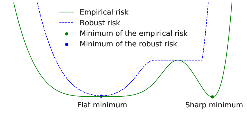
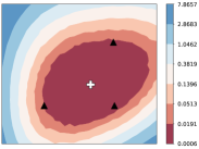
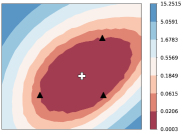
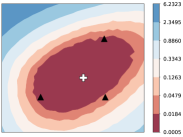
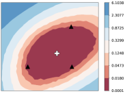
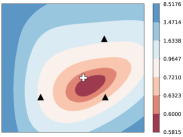
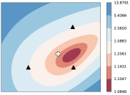
We consider a robust empirical loss function defined by the worst-case loss within neighborhoods in the parameter space as , where denotes the L2 norm and is a radius which defines neighborhoods of . Intuitively, if is sufficiently larger than the “radius” of a sharp optimum of , is no longer an optimum of as well as its neighborhoods within the -ball. On the other hand, if an optimum has larger “radius” than , there exists a local optimum within -ball – See Figure 1. Hence, solving the robust risk minimization (RRM), i.e., , will find a near solution of a flat optimum showing better generalizability [34, 26]. However, as domain shift worsen the generalization gap by breaking the i.i.d. assumption, it is not trivial that RRM will find an optimum with better DG performance. To answer the question, we first show the generalization bound between and as follows:
Theorem 1.
Consider a set of covers such that the parameter space where , and is dimension of . Let be a VC dimension of each . Then, for any , the following bound holds with probability at least ,
| (1) |
where is the number of the training samples and is a divergence between two distributions.
Proof can be done similarly as [37] and [34]. In Theorem 1, the test loss is bounded by three terms: (1) the robust empirical loss , (2) the discrepancy between training distribution and test distribution, i.e., the quantity of domain shift, and (3) a confidence bound related to the radius and the number of the training samples . Our theorem is similar to Ben-David et al. [37], while our theorem does not have the term related to the difference in labeling functions across the domains. It is because we simply assume there is no difference between labeling functions for each domain for simplicity. If one assumes a different labeling function, the dissimilarity term can be derived easily because it is independent and compatible with our main proof. More details of Theorem 1, including proof and discussions on the confidence bound, are in Appendix C.1 and C.2.
From Theorem 1, one can conjure that minimizing the robust empirical loss is directly related to the generalization performances on the target distribution. We show that the domain generalization gap on the target domain by the optimal solution of RRM, , is upper bounded as follows:
Theorem 2.
Let denote the optimal solution of the RRM, i.e., , and let be a VC dimension of the parameter space . Then, the gap between the optimal test loss, , and the test loss of , , has the following bound with probability at least .
| (2) | ||||
Proof is in Appendix C.3. It implies that if we find the optimal solution of the RRM (i.e., ), then the generalization gap in the test domain (i.e., ) is upper bounded by the gap between the RRM and ERM (i.e., ). Other terms in Theorem 2 are the discrepancy between the train domains and the target domain , and the confidence bounds caused by sample means. We remark that if we choose a proper , the optimal solution of the RRM will find a point near a flat optimum of ERM as shown in Figure 1. Hence, Theorem 2 and the intuition from Figure 1 imply that seeking a flat minimum of ERM will lead to a better domain generalization gap.
3 SWAD: Domain Generalization by Seeking Flat Minima
We have shown that flat minima will bring a better domain generalization. In this section, we propose Stochastic Weight Averaging Densely (SWAD) algorithm, and provide empirical quantitative and qualitative analyses on SWAD and flatness to understand why SWAD works better than ERM.
3.1 A baseline method: stochastic weight averaging
Since the importance of flatness in loss landscapes has emerged [23, 27, 24, 25, 28, 26], several methods have been proposed to find flat minima [26, 39, 25]. We select stochastic weight averaging (SWA) [25] as a baseline, which finds flat minima by a weight ensemble approach. More specifically, SWA updates a pretrained model (namely, a model trained with sufficiently enough training epochs, ) with a cyclical [40] or high constant learning rate scheduling. SWA gathers model parameters for every epochs during the update and averages them for the model ensemble. SWA finds an ensembled solution of different local optima found by a sufficiently large learning rate to escape a local minimum. Izmailov et al. [25] empirically showed that SWA finds flatter minima than ERM. We also considered sharpness-aware minimization (SAM) [26], which is another popular flatness-aware solver, but SWA finds flatter minima than SAM (See Figure 3). We illustrate an overview of SWA in Figure 2(a).
3.2 Dense and overfit-aware stochastic weight sampling strategy

Despite its advantages, directly applying SWA to DG task has two problems. First, SWA averages a few weights (usually less than ten) by sampling weights for every epochs, results in an inaccurate approximation of flat minima on a high-dimensional parameter space (e.g., 23M for ResNet-50 [41]). Furthermore, a common DG benchmark protocol uses relatively small training epochs (e.g., Gulrajani and Lopez-Paz [22] trained with less than two epochs for DomainNet benchmark), resulting in insufficient stochastic weights for SWA. From this motivation, we propose a “dense” sampling strategy for gathering sufficiently enough stochastic weights.
In addition, widely used DG datasets, such as PACS ( 10K images, 7 classes) and VLCS ( 11K images, 5 classes), are relatively smaller than large-scale datasets, such as ImageNet [42] ( 1.2M images, 1K classes). In this case, we observe that a simple ERM approach is rapidly reached to a local optimum only within a few epochs, and easily suffers from the overfitting issue, i.e., the validation loss is increased after a few training epochs. It implies that directly applying the vanilla SWA will suffer from the overfitting issue by averaging sub-optimal solutions (i.e., overfitted parameters). Hence, we need an “overfit-aware” sampling scheduling to omit the sub-optimal solutions for SWA.
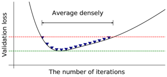
The main idea of Stochastic Weight Averaging Densely (SWAD) is a dense and overfit-aware stochastic weight gathering strategy. First, instead of collecting weights for every epochs, SWAD collects weights for every iteration. This dense sampling strategy easily collects sufficiently many weights than the sparse one. We also employ overfit-aware sampling scheduling by considering traces of the validation loss. Instead of sampling weights from pretraining epochs to the final epoch, we search the start iteration (when the validation loss achieves a local optimum for the first time) and the end iteration (when the validation loss is no longer decreased, but keep increasing). More specifically, we introduce three parameters: an optimum patient parameter , an overfitting patient parameter , and the tolerance rate for searching the start iteration and the end iteration . First, we search which satisfies , where denotes the validation loss at iteration . Simply, is the first iteration where the loss value is no longer decreased during iterations. Then, we find satisfying . In other words, is the first iteration where the validation loss values exceed the tolerance during iterations.
3.3 Empirical analysis of SWAD and flatness

|
Train |
 |
 |
 |
 |
|
Test |
 |
 |
 |
 |
| Art painting (test) | Cartoon (test) | Photo (test) | Sketch (test) |
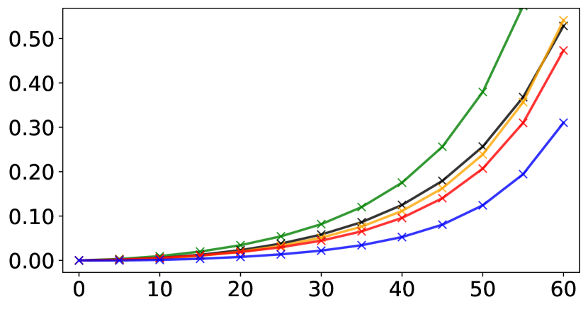
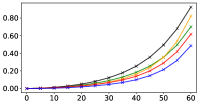
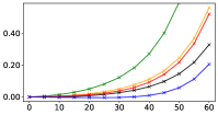
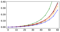
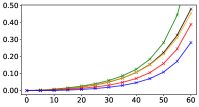
Here, we analyze solutions found by SWAD in terms of flatness. We first verify that the SWAD solution is flatter than those of ERM, SWA, and SAM. Our loss surface visualization shows that the SWAD solution is located on the center of the flat region, while ERM finds a boundary solution. Finally, we show that the sharp boundary solutions by ERM are not generalized well, resulting in sensitivity to the model selection. All following empirical analyses are conducted on PACS dataset, validating by all four domains (art painting, cartoon, photo, and sketch).
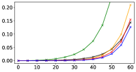
Local flatness anaylsis.
To begin with, we quantify the local flatness of a model parameter by assuming that flat minima will have smaller changes of loss value within its neighborhoods than sharp minima. For the given model parameter , we compute the expected loss value changes between and parameters on the sphere surrounding with radius , i.e., . In practice, is approximated by Monte-Carlo sampling with 100 samples. Note that the proposed local flatness is computationally efficient than measuring curvature using the Hessian-based quantities. Also, has an unbiased finite sample estimator, while the worst-case loss value, i.e., has no unbiased finite sample estimator.
In Figure 3, we compare of ERM, SAM, SWA with cyclic learning rate, SWA with constant learning rate, and SWAD by varying radius . SAM and SWA find the solutions with lower local flatness than ERM on average. SWAD finds the most flat minimum in every experiment.
|
Train |
 |
 |
 |
 |
|
Test |
 |
 |
 |
 |
| Art painting (test) | Cartoon (test) | Photo (test) | Sketch (test) |

Loss surface visualization.
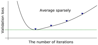
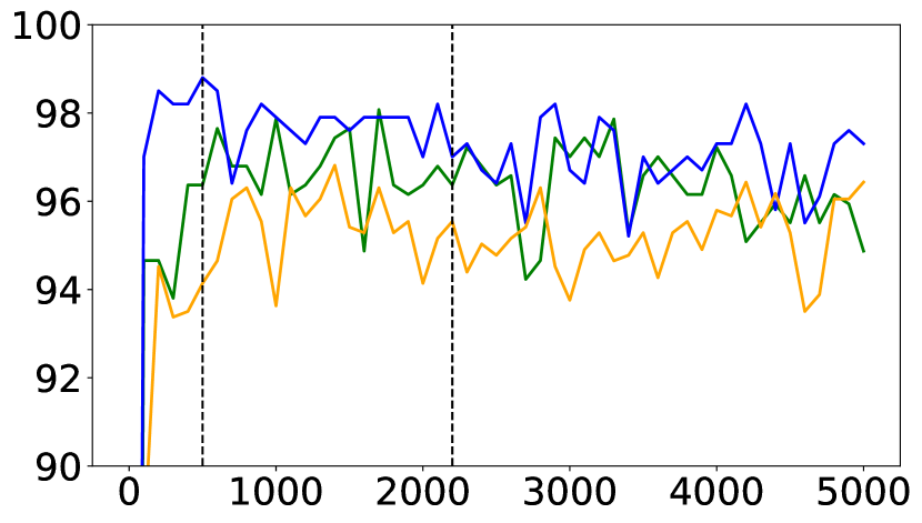
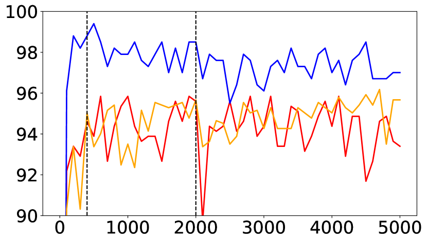
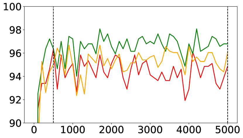
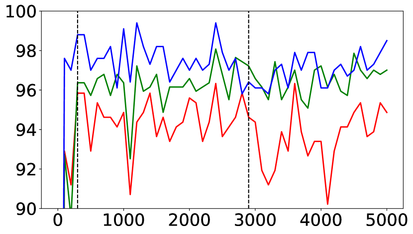
We visualize the loss landscapes by choosing three model weights on the optimization trajectory ()111We choose weights at iteration 2500, 3500, 4500 during the training., and computing the loss values by linear combinations of 222Each point is defined by two axes and computed by and . as [25]. More details are in Appendix B.5. In Figure 4, we observe that for all cases, ERM solutions are located at the boundary of a flat minimum of training loss, resulting in poor generalizability in test domains, that is aligned with our theoretical analysis and empirical flatness analysis. Since ERM solutions are located on the boundary of a flat loss surface, we observe that ERM solutions are very sensitive to model selection. In Figure 5, we illustrate the validation accuracies for each train-test domain combination of PACS by ERM, over training iterations (one epoch is equivalent to 83 iterations). We first observe that ERM rapidly reaches the best accuracy within only a few training epochs, namely less than 6 epochs. Furthermore, the ERM validation accuracies fluctuate a lot, and the final performance is very sensitive to the model selection criterion.
On the other hand, we observe that SWA solutions are located on the center of the training loss surfaces as well as of the test loss surfaces (Figure 4). Also, our overfit-aware stochastic weight gathering strategy (denoted as the vertical dot lines in Figure 5) prevents the ensembled weight from overfitting and makes SWAD model selection-free.
4 Experiments
4.1 Evaluation protocols
Dataset and optimization protocol. Following Gulrajani and Lopez-Paz [22], we exhaustively evaluate our method and comparison methods on various benchmarks: PACS [7] (9,991 images, 7 classes, and 4 domains), VLCS [43] (10,729 images, 5 classes, and 4 domains), OfficeHome [44] (15,588 images, 65 classes, and 4 domains), TerraIncognita [45] (24,788 images, 10 classes, and 4 domains), and DomainNet [46] (586,575 images, 345 classes, and 6 domains).
| Algorithm | PACS | VLCS | OfficeHome | TerraInc | DomainNet | Avg. |
| MASF [14] | 82.7 | - | - | - | - | - |
| DMG [33] | 83.4 | - | - | - | 43.6 | - |
| MetaReg [15] | 83.6 | - | - | - | 43.6 | - |
| ER [12] | 85.3 | - | - | - | - | - |
| pAdaIN [47] | 85.4 | - | - | - | - | - |
| EISNet [48] | 85.8 | - | - | - | - | - |
| DSON [30] | 86.6 | - | - | - | - | - |
| ERM† [29] | 85.5 | 77.5 | 66.5 | 46.1 | 40.9 | 63.3 |
| ERM (reproduced) | 84.2 | 77.3 | 67.6 | 47.8 | 44.0 | 64.2 |
| IRM† [20] | 83.5 | 78.6 | 64.3 | 47.6 | 33.9 | 61.6 |
| GroupDRO† [49] | 84.4 | 76.7 | 66.0 | 43.2 | 33.3 | 60.7 |
| I-Mixup† [50, 51, 52] | 84.6 | 77.4 | 68.1 | 47.9 | 39.2 | 63.4 |
| MLDG† [13] | 84.9 | 77.2 | 66.8 | 47.8 | 41.2 | 63.6 |
| CORAL† [31] | 86.2 | 78.8 | 68.7 | 47.7 | 41.5 | 64.5 |
| MMD† [53] | 84.7 | 77.5 | 66.4 | 42.2 | 23.4 | 58.8 |
| DANN† [9] | 83.7 | 78.6 | 65.9 | 46.7 | 38.3 | 62.6 |
| CDANN† [10] | 82.6 | 77.5 | 65.7 | 45.8 | 38.3 | 62.0 |
| MTL† [54] | 84.6 | 77.2 | 66.4 | 45.6 | 40.6 | 62.9 |
| SagNet† [32] | 86.3 | 77.8 | 68.1 | 48.6 | 40.3 | 64.2 |
| ARM† [16] | 85.1 | 77.6 | 64.8 | 45.5 | 35.5 | 61.7 |
| VREx† [21] | 84.9 | 78.3 | 66.4 | 46.4 | 33.6 | 61.9 |
| RSC† [55] | 85.2 | 77.1 | 65.5 | 46.6 | 38.9 | 62.7 |
| Mixstyle [17] | 85.2 | 77.9 | 60.4 | 44.0 | 34.0 | 60.3 |
| SWAD (ours) | 88.1 | 79.1 | 70.6 | 50.0 | 46.5 | 66.9 |
| () | () | () | () | () |
For a fair comparison, we follow training and evaluation protocol by Gulrajani and Lopez-Paz [22], including the dataset splits, hyperparameter (HP) search and model selection (while SWAD does not need it) on the validation set, and optimizer HP, except the HP search space and the number of iterations for DomainNet. We use a reduced HP search space to reduce the computational costs. We also tripled the number of iterations for DomainNet from 5,000 to 15,000 because we observe that 5,000 is not sufficient to convergence. We re-evaluate ERM with 15,000 iterations, and observe 3.1pp average performance improvement () in DomainNet. For training, we choose a domain as the target domain and use the remaining domains as the training domain where 20% samples are used for validation and model selection. ImageNet [42] trained ResNet-50 [41] is employed as the initial weight, and optimized by Adam [38] optimizer with a learning rate of 5e-5. We construct a mini-batch containing all domains where each domain has 32 images. We set SWAD HPs to 3, to 6, and to 1.2 for VLCS and 1.3 for the others by HP search on the validation sets. Additional implementation details, such as other HPs, are given in Appendix B.
Evaluation metrics. We report out-of-domain accuracies for each domain and their average, i.e., a model is trained and validated on training domains and evaluated on the unseen target domain. Each out-of-domain performance is an average of three different runs with different train-validation splits.
4.2 Main results
| Out-of-domain | In-domain | |
| ERM | 85.3 | 96.6 |
| EMA | 85.5(-) | 97.0() |
| SAM | 85.5(-) | 97.4() |
| Mixup | 84.8(-) | 97.3() |
| CutMix | 83.8() | 97.6() |
| VAT | 85.4(-) | 96.9() |
| -model | 83.5() | 96.8() |
| SWA | 85.9() | 97.1() |
| SWAD | 87.1() | 97.7() |
Comparison with domain generalization methods. We report the full out-of-domain performances on five DG benchmarks in Table 2. The full tables including out-of-domain accuracies for each domain are in Appendix E. In all experiments, our SWAD achieves significant performance gain against ERM as well as the previous best results: +2.6pp in PACS, +0.3pp in VLCS, +1.4pp in TerraIncognita, +1.9pp in OfficeHome, and +2.9pp in DomainNet comparing to the previous best results. We observe that SWAD provides two practical advantages comparing to previous methods. First, SWAD does not need any modification on training objectives or model architecture, i.e., it is universally applicable to any other methods. As an example, we show that SWAD actually improves the performances of other DG methods, such as CORAL [31] in Table 4. Moreover, as we discussed before, SWAD is free to the model selection, resulting in stable performances (i.e., small standard errors) on various benchmarks. Note that we only compare results with ResNet-50 backbone for a fair comparison. We describe the implementation details of each comparison method and the hyperparameter search protocol in Appendix B.
Comparison with conventional generalization methods. We also compare SWAD with other conventional generalization methods to show that the remarkable domain generalization gaps by SWAD is not achieved by better generalization, but by seeking flat minima. The comparison methods include flatness-aware optimization methods, such as SAM [26], ensemble methods, such as EMA [56], data augmentation methods, such as Mixup [35] and CutMix [36], and consistency regularization methods, such as VAT [57] and -model [58]. We also split in-domain datasets into training (60%), validation (20%), and test (20%) splits, while no in-domain test set used for Table 2. Every experiment is repeated three times.
The results are shown in Table 3. We observe that all conventional methods helps in-domain generalization, i.e., performing better than ERM on in-domain test set. However, their out-of-domain performances are similar to or even worse than ERM. For example, CutMix and -model improve in-domain performances by 1.0pp and 0.2pp but degrade out-of-domain performances by 1.5pp and 1.8pp. SAM, another method for seeking flat minima, slightly increases both in-domain and out-of-domain performances but the out-of-domain performance is not statistically significant. We will discuss performances of SAM in other benchmarks later. In contrast, the vanilla SWA and our SWAD significantly improve both in-domain and out-of-domain performances. SWAD improves the performances by SWA with statistically significantly gaps: 1.2pp on the out-of-domain and 0.6pp on the in-domain. Further comparison between SWA and SWAD is provided in §4.3.
| PACS | VLCS | OfficeHome | TerraInc | DomainNet | Avg. () | |
| ERM | 85.5 | 77.5 | 66.5 | 46.1 | 40.9 | 63.3 |
| ERM + SWA | 86.9 | 76.6 | 69.3 | 49.2 | 45.9 | 65.6 (+2.3) |
| ERM + SWAD | 88.1 | 79.1 | 70.6 | 50.0 | 46.5 | 66.9 (+3.6) |
| CORAL | 86.2 | 78.8 | 68.7 | 47.6 | 41.5 | 64.5 |
| CORAL + SWAD | 88.3 | 78.9 | 71.3 | 51.0 | 46.8 | 67.3 (+2.8) |
| SAM | 85.8 | 79.4 | 69.6 | 43.3 | 44.3 | 64.5 |
| SAM + SWAD | 87.1 | 78.5 | 69.9 | 45.3 | 46.5 | 65.5 (+1.0) |
Combinations with other methods. Since SWAD does not require any modification on training procedures and model architectures, SWAD is universally applicable to any other methods. Here, we combine SWAD with ERM, CORAL [31], and SAM [26]. Results are shown in Table 4. Both CORAL and SAM solely show better performances than ERM with +1.2pp average out-of-domain accuracy gap. Note that SAM is not a DG method but a sharpness-aware optimization method to find flat minima. It supports our theoretical motivation: DG can be achieved by seeking flat minima.
By applying SWAD on the baselines, the performances are consistently improved by 3.6pp on ERM, 2.8pp on CORAL, and 1.0pp on SAM. Interestingly, CORAL + SWAD show the best performances with both incorporating different advantages of utilizing domain labels and seeking flat minima. We also observe that SAM + SWAD shows worse performance than ERM + SWAD, while SAM performs better than ERM. We conjecture that it is because the objective control by SAM restricts the model parameter diversity durinig training, reducing the diversity for SWA ensemble. However, applying SWAD on SAM still leads to better performances than the sole SAM. The results demonstrate that the application of SWAD on other baselines is a simple yet effective method for DG.
4.3 Ablation study
| Configuration | Out-of-domain | In-domain | ||||||||
| lr | interval | PACS | VLCS | Avg. | PACS | VLCS | Avg. | |||
| SWA | 4000 | 5000 | Cyclic | 100 | 85.9 | 76.6 | 81.2 | 97.1 | 85.0 | 91.0 |
| SWA | 4000 | 5000 | Const | 100 | 86.5 | 76.7 | 81.6 | 97.3 | 85.0 | 91.1 |
| SWAD | Opt | Overfit | Const | 100 | 86.5 | 78.0 | 82.2 | 97.6 | 85.8 | 91.7 |
| SWAD | 4000 | 5000 | Const | 1 | 86.6 | 76.9 | 81.7 | 97.5 | 85.2 | 91.3 |
| SWAD | Opt | 5000 | Const | 1 | 87.1 | 77.6 | 82.4 | 97.7 | 85.8 | 91.8 |
| SWAD | Val | Val | Const | 1 | 86.2 | 78.6 | 82.4 | 97.5 | 85.8 | 91.7 |
| SWAD (proposed) | Opt | Overfit | Const | 1 | 87.1 | 78.9 | 83.0 | 97.7 | 86.1 | 91.9 |
Table 5 provides ablative studies on the starting and ending iterations for averaging, the learning rate schedule, and the sampling interval. SWA (SWA in Table 3) and SWA are vanilla SWAs with fixed sampling positions. We also report SWAD by eliminating three factors: the dense sampling strategy, and searching the start iteration, searching the end iteration. The dense sampling strategy lets SWAD estimate a more accurate approximation of flat minima: showing 0.8pp degeneration in the average out-of-domain accuracy (SWAD). When we take an average from to the final iteration, the out-of-domain performance degrades by 0.6pp (SWAD). Similarly, a fixed scheduling without the overfit-aware scheduling only shows very marginal improvements from the vanilla SWA (SWAD). We also evaluate SWAD that uses the range achieving the best performances on the validation set, but it becomes overfitted to the validation, results in lower performances than SWAD. The results demonstrate the benefits of combining “dense” and “overfit-aware” sampling strategies of SWAD.
4.4 Exploring the other applications: ImageNet robustness
| Method | ImageNet (%) ↑ | ImageNet-C (mCE) ↓ | BGC (%) ↑ | ImageNet-R (%) ↑ |
| ERM | 76.5 | 57.6 | 8.7 | 36.7 |
| SWA | 76.9 | 56.8 | 10.9 | 37.5 |
| SWAD (ours) | 77.0 | 55.7 | 11.8 | 38.8 |
Since SWAD does not rely on domain labels, it can be applied to other robustness tasks not containing domain labels. Table 6 show the generalizability of SWAD on ImageNet [42] and its shifted benchmarks, namely, ImageNet-C [59], ImageNet-R [60], and background challenge (BGC) [61]. SWAD consistently improves robustness performances against the ERM baseline and the SWA baseline. These results support that our method is robustly and widely applicable to improve both in-domain and out-of-domain generalizability. The detailed setup is provided in Appendix B.6.
5 Discussion and Limitations
Despite many benefits from SWAD, such as the significant performance improvements, model selection-free property, working plug-and-play manner for various methods, there are some potential limitations. Here, we discuss the limitations of SWAD for further improvements.
Confidence error in Theorem 1. While the confidence error in Theorem 1 tells the effect of on generalization error bound, there exists a limitation in that the confidence error term shows improper behavior with respect to if is close to zero. The behavior we expect is that the confidence error of RRM converges to the confidence error of ERM as decreases to zero, however, the current theorem does not show such tendency since the confidence bound diverges to infinity when goes to zero. However, we would like to note that this limitation is not a drawback of RRM, but it is caused by the looseness of the union bound which is a mathematical technique used to derive the confidence error of RRM. Our RRM formulation has a similarity to previous works [34, 26] and we note that the counter-intuitive behavior of the confidence bound and also appears in Foret et al. [26].
SWAD is not a perfect flatness-aware optimization method. Note that SWAD is not a perfect and theoretically guaranteed solver for flat minima, but a heuristic approximation with empirical benefits. However, even if a better flatness-aware optimization method is proposed, our theoretical contribution still holds: showing the relationship between flat minima and DG.
SWAD does not strongly utilize domain-specific information. In Theorem 2, the domain generalization gap is bounded by three factors: flat minima, domain discrepancy, and confidence bound. Most of the existing approaches focus on domain discrepancy, reducing the difference between the source domains and the target domain by domain invariant learning [8, 9, 10, 11, 12]. SWAD focuses on the first factor, the flat minima. While the domain labels are used to construct a mini-batch, SWAD does not strongly utilize domain-specific information. It implies that if one can consider both flatness and domain discrepancy, better domain generalization can be achievable. Table 4 gives us a clue: the combination of CORAL (utilizing domain-specific information) and SWAD (seeking flat minima) shows the best performance among all comparison methods. As a future research direction, we encourage studying a method that can achieve both flat optima and small domain discrepancy.
6 Concluding Remarks
In this paper, we theoretically and empirically demonstrate that domain generalization (DG) is achievable by seeking flat minima. We propose SWAD that captures flatter minima than the vanilla SWA does. The extensive experiments on five DG benchmarks show superior performances of SWAD compared with existing DG methods. In addition, combinations of SWAD and existing DG methods even show better performances than the vanilla SWAD. We theoretically and empirically observe that seeking flat minima can achieve better generalizability to both in-domain and out-of-domain, while strong in-domain generalization methods without consideration of flatness, e.g., Mixup or CutMix, cannot guarantee to achieve out-of-domain generalizability in both theory and practice. This study first brings the concept of flatness into DG tasks, and shows strong empirical performances not only in DG but also in ImageNet benchmarks. We hope that this study promotes a new research direction of seeking flat minima for domain generalization and other robustness tasks.
Acknowledgments and Disclosure of Funding
NAVER Smart Machine Learning (NSML) [62] and Kakao Brain Cloud platform have been used in experiments. This work was supported by IITP grant funded by the Korea government (MSIT) (No. 2021-0-01341, AI Graduate School Program, CAU).
References
- Dai and Van Gool [2018] Dengxin Dai and Luc Van Gool. Dark model adaptation: Semantic image segmentation from daytime to nighttime. In 2018 21st International Conference on Intelligent Transportation Systems (ITSC), pages 3819–3824. IEEE, 2018.
- Michaelis et al. [2019] Claudio Michaelis, Benjamin Mitzkus, Robert Geirhos, Evgenia Rusak, Oliver Bringmann, Alexander S Ecker, Matthias Bethge, and Wieland Brendel. Benchmarking robustness in object detection: Autonomous driving when winter is coming. arXiv preprint arXiv:1907.07484, 2019.
- de Vries et al. [2019] Terrance de Vries, Ishan Misra, Changhan Wang, and Laurens van der Maaten. Does object recognition work for everyone? In Proceedings of the IEEE/CVF Conference on Computer Vision and Pattern Recognition Workshops, pages 52–59, 2019.
- Yang et al. [2020] Kaiyu Yang, Klint Qinami, Li Fei-Fei, Jia Deng, and Olga Russakovsky. Towards fairer datasets: Filtering and balancing the distribution of the people subtree in the imagenet hierarchy. In Proceedings of the 2020 Conference on Fairness, Accountability, and Transparency, pages 547–558, 2020.
- Geirhos et al. [2019] Robert Geirhos, Patricia Rubisch, Claudio Michaelis, Matthias Bethge, Felix A. Wichmann, and Wieland Brendel. Imagenet-trained cnns are biased towards texture; increasing shape bias improves accuracy and robustness. In International Conference on Learning Representations, 2019.
- Beery et al. [2018a] Sara Beery, Grant Van Horn, and Pietro Perona. Recognition in terra incognita. In Proceedings of the European Conference on Computer Vision (ECCV), pages 456–473, 2018a.
- Li et al. [2017] Da Li, Yongxin Yang, Yi-Zhe Song, and Timothy M Hospedales. Deeper, broader and artier domain generalization. In IEEE International Conference on Computer Vision, pages 5542–5550, 2017.
- Muandet et al. [2013] Krikamol Muandet, David Balduzzi, and Bernhard Schölkopf. Domain generalization via invariant feature representation. In International Conference on Machine Learning, pages 10–18. PMLR, 2013.
- Ganin et al. [2016] Yaroslav Ganin, Evgeniya Ustinova, Hana Ajakan, Pascal Germain, Hugo Larochelle, François Laviolette, Mario Marchand, and Victor Lempitsky. Domain-adversarial training of neural networks. Journal of machine learning research, 17(1):2096–2030, 2016.
- Li et al. [2018a] Ya Li, Mingming Gong, Xinmei Tian, Tongliang Liu, and Dacheng Tao. Domain generalization via conditional invariant representations. In AAAI Conference on Artificial Intelligence, volume 32, 2018a.
- Bahng et al. [2020] Hyojin Bahng, Sanghyuk Chun, Sangdoo Yun, Jaegul Choo, and Seong Joon Oh. Learning de-biased representations with biased representations. In International Conference on Machine Learning (ICML), 2020.
- Zhao et al. [2020] Shanshan Zhao, Mingming Gong, Tongliang Liu, Huan Fu, and Dacheng Tao. Domain generalization via entropy regularization. Neural Information Processing Systems, 33, 2020.
- Li et al. [2018b] Da Li, Yongxin Yang, Yi-Zhe Song, and Timothy Hospedales. Learning to generalize: Meta-learning for domain generalization. In AAAI Conference on Artificial Intelligence, volume 32, 2018b.
- Dou et al. [2019] Qi Dou, Daniel C Castro, Konstantinos Kamnitsas, and Ben Glocker. Domain generalization via model-agnostic learning of semantic features. Neural Information Processing System, 2019.
- Balaji et al. [2018] Yogesh Balaji, Swami Sankaranarayanan, and Rama Chellappa. Metareg: Towards domain generalization using meta-regularization. Neural Information Processing Systems, 31:998–1008, 2018.
- Zhang et al. [2020] Marvin Zhang, Henrik Marklund, Abhishek Gupta, Sergey Levine, and Chelsea Finn. Adaptive risk minimization: A meta-learning approach for tackling group shift. arXiv preprint arXiv:2007.02931, 2020.
- Zhou et al. [2021] Kaiyang Zhou, Yongxin Yang, Yu Qiao, and Tao Xiang. Domain generalization with mixstyle. In International Conference on Learning Representations, 2021.
- Shankar et al. [2018] Shiv Shankar, Vihari Piratla, Soumen Chakrabarti, Siddhartha Chaudhuri, Preethi Jyothi, and Sunita Sarawagi. Generalizing across domains via cross-gradient training. In International Conference on Learning Representations, 2018.
- Carlucci et al. [2019] Fabio M Carlucci, Antonio D’Innocente, Silvia Bucci, Barbara Caputo, and Tatiana Tommasi. Domain generalization by solving jigsaw puzzles. In IEEE/CVF Conference on Computer Vision and Pattern Recognition, pages 2229–2238, 2019.
- Arjovsky et al. [2019] Martin Arjovsky, Léon Bottou, Ishaan Gulrajani, and David Lopez-Paz. Invariant risk minimization. arXiv preprint arXiv:1907.02893, 2019.
- Krueger et al. [2020] David Krueger, Ethan Caballero, Joern-Henrik Jacobsen, Amy Zhang, Jonathan Binas, Remi Le Priol, and Aaron Courville. Out-of-distribution generalization via risk extrapolation (rex). arXiv preprint arXiv:2003.00688, 2020.
- Gulrajani and Lopez-Paz [2021] Ishaan Gulrajani and David Lopez-Paz. In search of lost domain generalization. In International Conference on Learning Representations, 2021.
- Keskar et al. [2017] Nitish Shirish Keskar, Dheevatsa Mudigere, Jorge Nocedal, Mikhail Smelyanskiy, and Ping Tak Peter Tang. On large-batch training for deep learning: Generalization gap and sharp minima. In International Conference on Learning Representations, 2017.
- Garipov et al. [2018] Timur Garipov, Pavel Izmailov, Dmitrii Podoprikhin, Dmitry P Vetrov, and Andrew Gordon Wilson. Loss surfaces, mode connectivity, and fast ensembling of dnns. In Neural Information Processing Systems, 2018.
- Izmailov et al. [2018] Pavel Izmailov, Dmitrii Podoprikhin, Timur Garipov, Dmitry Vetrov, and Andrew Gordon Wilson. Averaging weights leads to wider optima and better generalization. Conference on Uncertainty in Artificial Intelligence, 2018.
- Foret et al. [2021] Pierre Foret, Ariel Kleiner, Hossein Mobahi, and Behnam Neyshabur. Sharpness-aware minimization for efficiently improving generalization. In International Conference on Learning Representations, 2021.
- Dziugaite and Roy [2017] Gintare Karolina Dziugaite and Daniel M Roy. Computing nonvacuous generalization bounds for deep (stochastic) neural networks with many more parameters than training data. In Uncertainty in Artificial Intelligence, 2017.
- Jiang et al. [2019] Yiding Jiang, Behnam Neyshabur, Hossein Mobahi, Dilip Krishnan, and Samy Bengio. Fantastic generalization measures and where to find them. arXiv preprint arXiv:1912.02178, 2019.
- Vapnik [1998] V Vapnik. Statistical learning theory. NY: Wiley, 1998.
- Seo et al. [2020] Seonguk Seo, Yumin Suh, Dongwan Kim, Jongwoo Han, and Bohyung Han. Learning to optimize domain specific normalization for domain generalization. European Conference on Computer Vision, 2020.
- Sun and Saenko [2016] Baochen Sun and Kate Saenko. Deep coral: Correlation alignment for deep domain adaptation. In European conference on computer vision, pages 443–450. Springer, 2016.
- Nam et al. [2021] Hyeonseob Nam, HyunJae Lee, Jongchan Park, Wonjun Yoon, and Donggeun Yoo. Reducing domain gap by reducing style bias. In Proceedings of the IEEE/CVF Conference on Computer Vision and Pattern Recognition, pages 8690–8699, 2021.
- Chattopadhyay et al. [2020] Prithvijit Chattopadhyay, Yogesh Balaji, and Judy Hoffman. Learning to balance specificity and invariance for in and out of domain generalization. In European Conference on Computer Vision, pages 301–318. Springer, 2020.
- Norton and Royset [2019] Matthew Norton and Johannes O Royset. Diametrical risk minimization: Theory and computations. arXiv preprint arXiv:1910.10844, 2019.
- Zhang et al. [2018] Hongyi Zhang, Moustapha Cisse, Yann N. Dauphin, and David Lopez-Paz. mixup: Beyond empirical risk minimization. International Conference on Learning Representations, 2018.
- Yun et al. [2019] Sangdoo Yun, Dongyoon Han, Seong Joon Oh, Sanghyuk Chun, Junsuk Choe, and Youngjoon Yoo. Cutmix: Regularization strategy to train strong classifiers with localizable features. In International Conference on Computer Vision (ICCV), 2019.
- Ben-David et al. [2010] Shai Ben-David, John Blitzer, Koby Crammer, Alex Kulesza, Fernando Pereira, and Jennifer Wortman Vaughan. A theory of learning from different domains. Machine learning, 79(1):151–175, 2010.
- Kingma and Ba [2015] Diederik P Kingma and Jimmy Ba. Adam: A method for stochastic optimization. In International Conference on Learning Representations, 2015.
- Chaudhari et al. [2019] Pratik Chaudhari, Anna Choromanska, Stefano Soatto, Yann LeCun, Carlo Baldassi, Christian Borgs, Jennifer Chayes, Levent Sagun, and Riccardo Zecchina. Entropy-sgd: Biasing gradient descent into wide valleys. Journal of Statistical Mechanics: Theory and Experiment, 2019(12):124018, 2019.
- Smith [2017] Leslie N Smith. Cyclical learning rates for training neural networks. In 2017 IEEE winter conference on applications of computer vision (WACV), pages 464–472. IEEE, 2017.
- He et al. [2016] Kaiming He, Xiangyu Zhang, Shaoqing Ren, and Jian Sun. Deep residual learning for image recognition. In IEEE Conference on Computer Vision and Pattern Recognition, 2016.
- Russakovsky et al. [2015] Olga Russakovsky, Jia Deng, Hao Su, Jonathan Krause, Sanjeev Satheesh, Sean Ma, Zhiheng Huang, Andrej Karpathy, Aditya Khosla, Michael Bernstein, et al. Imagenet large scale visual recognition challenge. International Journal of Computer Vision, 115(3):211–252, 2015.
- Fang et al. [2013] Chen Fang, Ye Xu, and Daniel N Rockmore. Unbiased metric learning: On the utilization of multiple datasets and web images for softening bias. In IEEE International Conference on Computer Vision, pages 1657–1664, 2013.
- Venkateswara et al. [2017] Hemanth Venkateswara, Jose Eusebio, Shayok Chakraborty, and Sethuraman Panchanathan. Deep hashing network for unsupervised domain adaptation. In IEEE conference on computer vision and pattern recognition, pages 5018–5027, 2017.
- Beery et al. [2018b] Sara Beery, Grant Van Horn, and Pietro Perona. Recognition in terra incognita. In European Conference on Computer Vision, pages 456–473, 2018b.
- Peng et al. [2019] Xingchao Peng, Qinxun Bai, Xide Xia, Zijun Huang, Kate Saenko, and Bo Wang. Moment matching for multi-source domain adaptation. In IEEE/CVF International Conference on Computer Vision, pages 1406–1415, 2019.
- Nuriel et al. [2021] Oren Nuriel, Sagie Benaim, and Lior Wolf. Permuted adain: Reducing the bias towards global statistics in image classification. In IEEE/CVF Conference on Computer Vision and Pattern Recognition, 2021.
- Wang et al. [2020a] Shujun Wang, Lequan Yu, Caizi Li, Chi-Wing Fu, and Pheng-Ann Heng. Learning from extrinsic and intrinsic supervisions for domain generalization. In European Conference on Computer Vision, pages 159–176. Springer, 2020a.
- Sagawa* et al. [2020] Shiori Sagawa*, Pang Wei Koh*, Tatsunori B. Hashimoto, and Percy Liang. Distributionally robust neural networks. In International Conference on Learning Representations, 2020.
- Xu et al. [2020] Minghao Xu, Jian Zhang, Bingbing Ni, Teng Li, Chengjie Wang, Qi Tian, and Wenjun Zhang. Adversarial domain adaptation with domain mixup. In AAAI Conference on Artificial Intelligence, volume 34, pages 6502–6509, 2020.
- Yan et al. [2020] Shen Yan, Huan Song, Nanxiang Li, Lincan Zou, and Liu Ren. Improve unsupervised domain adaptation with mixup training. arXiv preprint arXiv:2001.00677, 2020.
- Wang et al. [2020b] Yufei Wang, Haoliang Li, and Alex C Kot. Heterogeneous domain generalization via domain mixup. In IEEE International Conference on Acoustics, Speech and Signal Processing, pages 3622–3626. IEEE, 2020b.
- Li et al. [2018c] Haoliang Li, Sinno Jialin Pan, Shiqi Wang, and Alex C Kot. Domain generalization with adversarial feature learning. In IEEE Conference on Computer Vision and Pattern Recognition, pages 5400–5409, 2018c.
- Blanchard et al. [2021] Gilles Blanchard, Aniket Anand Deshmukh, Urun Dogan, Gyemin Lee, and Clayton Scott. Domain generalization by marginal transfer learning. Journal of Machine Learning Research, 22(2):1–55, 2021.
- Huang et al. [2020] Zeyi Huang, Haohan Wang, Eric P Xing, and Dong Huang. Self-challenging improves cross-domain generalization. European Conference on Computer Vision, 2, 2020.
- Polyak and Juditsky [1992] Boris T Polyak and Anatoli B Juditsky. Acceleration of stochastic approximation by averaging. SIAM journal on control and optimization, 30(4):838–855, 1992.
- Miyato et al. [2018] Takeru Miyato, Shin-ichi Maeda, Masanori Koyama, and Shin Ishii. Virtual adversarial training: a regularization method for supervised and semi-supervised learning. IEEE Transactions on Pattern Analysis and Machine Intelligence, 41(8):1979–1993, 2018.
- Laine and Aila [2017] Samuli Laine and Timo Aila. Temporal ensembling for semi-supervised learning. In International Conference on Learning Representations, 2017.
- Hendrycks and Dietterich [2018] Dan Hendrycks and Thomas Dietterich. Benchmarking neural network robustness to common corruptions and perturbations. In International Conference on Learning Representations, 2018.
- Hendrycks et al. [2020] Dan Hendrycks, Steven Basart, Norman Mu, Saurav Kadavath, Frank Wang, Evan Dorundo, Rahul Desai, Tyler Zhu, Samyak Parajuli, Mike Guo, et al. The many faces of robustness: A critical analysis of out-of-distribution generalization. arXiv preprint arXiv:2006.16241, 2020.
- Xiao et al. [2020] Kai Yuanqing Xiao, Logan Engstrom, Andrew Ilyas, and Aleksander Madry. Noise or signal: The role of image backgrounds in object recognition. In International Conference on Learning Representations, 2020.
- Kim et al. [2018] Hanjoo Kim, Minkyu Kim, Dongjoo Seo, Jinwoong Kim, Heungseok Park, Soeun Park, Hyunwoo Jo, KyungHyun Kim, Youngil Yang, Youngkwan Kim, et al. Nsml: Meet the mlaas platform with a real-world case study. arXiv preprint arXiv:1810.09957, 2018.
- Goyal et al. [2017] Priya Goyal, Piotr Dollár, Ross Girshick, Pieter Noordhuis, Lukasz Wesolowski, Aapo Kyrola, Andrew Tulloch, Yangqing Jia, and Kaiming He. Accurate, large minibatch sgd: Training imagenet in 1 hour. arXiv preprint arXiv:1706.02677, 2017.
- Zhao et al. [2018] Han Zhao, Shanghang Zhang, Guanhang Wu, José M. F. Moura, Joao P Costeira, and Geoffrey J Gordon. Adversarial multiple source domain adaptation. In Advances in Neural Information Processing Systems, volume 31, 2018.
Appendix A Potential Societal Impacts
In this study, we theoretically and empirically demonstrate that domain generalization (DG) is achievable by seeking flat minima, and propose SWAD to find flat minima. With SWAD, researchers and developers can make a model robust to domain shift in a real deployment environment, without relying on a task-dependent prior, a modified objective function, or a specific model architecture. Accordingly, SWAD has potential positive impacts by developing machines less biased towards ethical aspects, as well as potential negative impacts, e.g., improving weapon or surveillance systems under unexpected environment changes.
Appendix B Implementation Details
B.1 Hyperparameters of SWAD
The evaluation protocol by Gulrajani and Lopez-Paz [22] is computationally too expensive; it requires about 4,142 models for every DG algorithm. Hence, we reduce the search space of SWAD for computational efficiency; batch size and learning rate are set to 32 for each domain and 5e-5, respectively. We set dropout probability and weight decay to zero. We only search and . and are searched in PACS dataset, and the searched values are used for all experiments, while is searched in [1.2, 1.3] depending on dataset. As a result, we use , , and for VLCS and for the others. We initialize our model by ImageNet-pretrained ResNet-50 and batch normalization statistics are frozen during training. The number of total iterations is for DomainNet and for others, which are sufficient numbers to be converged. Finally, we slightly modify the evaluation frequency because it should be set to small enough to detect the moments that the model is optimized and overfitted. However, too small frequency brings large evaluation overhead, thus we compromise between exactness and efficiency: for VLCS, for DomainNet, and for others.
B.2 Hyperparameter search protocol for reproduced results
| Parameter | Default value | DomainBed | Ours |
| batch size | 32 | 32 | |
| learning rate | 5e-5 | [1e-5, 3e-5, 5e-5] | |
| ResNet dropout | 0 | [0.0, 0.1, 0.5] | [0.0, 0.1, 0.5] |
| weight decay | 0 | [1e-4, 1e-6] |
We evaluate recently proposed methods, SAM [26] and Mixstyle [17], and compare them with previous results. For a fair comparison, we follow the hyperparameter (HP) search protocol proposed by Gulrajani and Lopez-Paz [22], with a modification to reduce computational resources. They searched HP by training a total of 58,000 models, corresponding to about 4,142 runs for each algorithm. It is too much computational burden to train 4,142 models whenever evaluate a new algorithm. Therefore, we re-design the HP search protocol efficiently and effectively. In the HP search protocol of DomainBed [22], training domains and algorithm-specific parameters are included in the HP search space, and HP is found for every data split independently by random search. Instead, we do not sample training domains, use HP found in the first data split to the other splits, search algorithm-specific HP independently, and conduct grid search on the more effectively designed HP space as shown in Table 7. Through the proposed protocol, we find HP for an algorithm under only 396 runs. Although the number of total runs is reduced to about 10% (), the results of reproduced ERM is improved 0.9pp in average (). It demonstrates both the effectiveness and the efficiency of our search protocol.
B.3 Algorithm-specific hyperparameters
We search the algorithm-specific hyperparameters independently in PACS dataset, based on the values suggested from each paper. For Mixstyle [17], we insert Mixstyle block with domain label after the 1st, 2nd, and 3rd residual blocks with and . We train SAM [26] with , and VAT [57] with and . In -model [58], is chosen among various values such as 1, 10, 100, and 300. We use EMA [56] with , Mixup [35] with , and CutMix [36] with and .
B.4 Pseudo code
B.5 Loss surface visualization
Following Garipov et al. [24], we choose three model weights and define two dimensional weight plane from the weights:
| (3) |
where and are orthonormal bases of the weight plane. Then, we build Cartesian grid near the weights on the plane. For each grid point, we calculate the weight corresponding to the point and compute loss from the weight. The results are visualized as a contour plot, as shown in Figure 4 in the main text.
B.6 ImageNet robustness experiments
We investigate the extensibility of SWAD via three robustness benchmarks (Section 4.4 in the main text), namely ImageNet-C [59], ImageNet-R [60], and background challenge (BGC) [61]. ImageNet-C measures the robustness against common corruptions such as Gaussian noise, blur, or weather changes. We follow Hendrycks and Dietterich [59] for measuring mean corruption error (mCE). The lower ImageNet-C implies that the model is robust against corruption noises. BGC evaluates the robustness against background manipulations as well as the adversarial robustness. The BGC dataset has two groups, foreground and background. BGC manipulates images by combining the foregrounds and backgrounds, and measures whether the model predicts a consistent prediction with any manipulated image. ImageNet-R tests the robustness against different domains. ImageNet-R collects very different domain images of ImageNet, such as art, cartoons, deviantart, graffiti, embroidery, graphics, origami, paintings, patterns, plastic objects, plush objects, sculptures, sketches, tattoos, toys, and video game renditions. Showing better performances in ImageNet-R leads to the same conclusion as other domain generalization benchmarks.
Experiment details.
We use ResNet-50 architecture and mostly follow standard training recipes. We use SGD optimizer with momentum of 0.9, base learning rate of 0.1 with linear scaling rule [63] and polynomial decay, 5 epochs gradual warmup, batch size of 2048, and total epochs of 90. For SWA, the learning rate is decayed to 1/20 until of training (72 epochs), and the cyclic learning rate with 3 epochs cycle length is used for the left of training. SWAD follows the same learning rate decay until of training, but averages every weight from every iteration after of training with constant learning rate.
Appendix C Proof of Theorems
C.1 Technical Lemmas
Consider an instance loss function such that and if and only if . Then, we can define a functional error as . Note that if we set as a true label function which generates the label of inputs, , then, it becomes a population loss . Given two distributions, and , the following lemma shows that the difference between the error with and the error with is bounded by the divergence between and .
Lemma 1.
Proof.
We employ the same technique in Zhao et al. [64] for our loss function . From the Fubini’s theorem, we have,
| (4) |
By using this fact,
| (5) | |||
| (6) | |||
| (7) | |||
| (8) | |||
| (9) | |||
| (10) | |||
| (11) |
where . ∎
Lemma 2.
Consider a distribution on input space and global label function . Let be a finite cover of a parameter space which consists of closed balls with radius where . Let be a local maximum in the -th ball. Let a VC dimension of be . Then, for any , the following bound holds with probability at least .
| (12) |
where is an empirical robust risk with samples.
Proof.
We first show that the following inequality holds for the local maximum of covers,
| (13) | ||||
| (14) | ||||
| (15) |
Now, we introduce a confidence error bound . Then, we set . Then, we get,
| (16) | ||||
| (17) | ||||
| (18) |
since for all . Hence, the inequality holds with probability at least .
Based on this fact, let us consider the set of events such that . Then, for any , there exists such that . Then, we get
| (19) | ||||
| (20) | ||||
| (21) |
where the second inequality holds since and the final inequality holds since is the local maximum in . In this regards, we know that implies . Consequently, holds with probability at least . ∎
C.2 Proof of Theorem 1
Proof.
The proof consists of two parts. First, we show that the following inequality holds with high probability.
Then, secondly, we apply the inequality for multiple source domains.
The first part can be proven by simply combining Lemma 1 and Lemma 2. Then, we get,
| (22) | ||||
| (23) |
where is a divergence between and .
For the second part, we set which is a mixture of source distributions. Then, by applying to the first part, we obtain the following inequality,
| (24) | ||||
| (25) |
where the total number of training data set is and, for the second inequality, we use the fact that , which has been proven in [64]. ∎
C.3 Proof of Theorem 2
Proof.
First, let . Then, from generalization error bound of , the following inequality holds with probability at most ,
| (26) |
where is a VC dimension of . Furthermore, from Theorem 1, we have the following inequality with probability at most ,
| (27) |
Finally, let us consider the set of event such that and whose probability is at least greater than . Then, under this set of event, we have,
| (28) | ||||
| (29) | ||||
| (30) |
Consequently, we have,
| (31) | ||||
| (32) |
∎
Appendix D Additional Experiments
D.1 Comparison of flatness-aware solvers
| Algorithm | PACS | VLCS | OfficeHome | TerraInc | DomainNet | Avg. |
| ERM (baseline) | 85.5 | 77.5 | 66.5 | 46.1 | 40.9 | 63.3 |
| SAM | 85.8 | 79.4 | 69.6 | 43.3 | 44.3 | 64.5 |
| SWA | 87.1 | 76.5 | 68.5 | 49.6 | 45.6 | 65.5 |
| SWA | 86.9 | 76.6 | 69.3 | 49.2 | 45.9 | 65.6 |
| SWAD | 88.1 | 79.1 | 70.6 | 50.0 | 46.5 | 66.9 |
Interestingly, the average performance ranking of flatness-aware solvers is the same as the results of the local flatness test (See Figure 3 in the main text). In both experiments, SWAD performs best, followed by SWAs, SAM, and ERM. It is another evidence of our claim that domain generalization is achievable by seeking flat minima.
On the other hand, comparing SWAs and SWAD demonstrates the effectiveness of the proposed dense and overfit-aware sampling strategy. SWAD improves average performance up to 1.4pp, and surpasses both SWAs on every benchmark.
Appendix E Full Results
In this section, we show detailed results of Table 2 in the main text. and indicate results from DomainBed’s and our HP search protocols, respectively. Standard errors are reported from three trials, if available.
E.1 PACS
| Algorithm | A | C | P | S | Avg |
| CDANN† | 84.6 | 75.5 | 96.8 | 73.5 | 82.6 |
| MASF | 82.9 | 80.5 | 95.0 | 72.3 | 82.7 |
| DMG | 82.6 | 78.1 | 94.5 | 78.3 | 83.4 |
| IRM† | 84.8 | 76.4 | 96.7 | 76.1 | 83.5 |
| MetaReg | 87.2 | 79.2 | 97.6 | 70.3 | 83.6 |
| DANN† | 86.4 | 77.4 | 97.3 | 73.5 | 83.7 |
| ERM‡ | 85.7 | 77.1 | 97.4 | 76.6 | 84.2 |
| GroupDRO† | 83.5 | 79.1 | 96.7 | 78.3 | 84.4 |
| MTL† | 87.5 | 77.1 | 96.4 | 77.3 | 84.6 |
| I-Mixup | 86.1 | 78.9 | 97.6 | 75.8 | 84.6 |
| MMD† | 86.1 | 79.4 | 96.6 | 76.5 | 84.7 |
| VREx† | 86.0 | 79.1 | 96.9 | 77.7 | 84.9 |
| MLDG† | 85.5 | 80.1 | 97.4 | 76.6 | 84.9 |
| ARM† | 86.8 | 76.8 | 97.4 | 79.3 | 85.1 |
| RSC† | 85.4 | 79.7 | 97.6 | 78.2 | 85.2 |
| Mixstyle‡ | 86.8 | 79.0 | 96.6 | 78.5 | 85.2 |
| ER | 87.5 | 79.3 | 98.3 | 76.3 | 85.3 |
| pAdaIN | 85.8 | 81.1 | 97.2 | 77.4 | 85.4 |
| ERM† | 84.7 | 80.8 | 97.2 | 79.3 | 85.5 |
| EISNet | 86.6 | 81.5 | 97.1 | 78.1 | 85.8 |
| CORAL† | 88.3 | 80.0 | 97.5 | 78.8 | 86.2 |
| SagNet† | 87.4 | 80.7 | 97.1 | 80.0 | 86.3 |
| DSON | 87.0 | 80.6 | 96.0 | 82.9 | 86.6 |
| Ours | 89.3 | 83.4 | 97.3 | 82.5 | 88.1 |
E.2 VLCS
| Algorithm | C | L | S | V | Avg |
| GroupDRO† | 97.3 | 63.4 | 69.5 | 76.7 | 76.7 |
| RSC† | 97.9 | 62.5 | 72.3 | 75.6 | 77.1 |
| MLDG† | 97.4 | 65.2 | 71.0 | 75.3 | 77.2 |
| MTL† | 97.8 | 64.3 | 71.5 | 75.3 | 77.2 |
| ERM‡ | 98.0 | 64.7 | 71.4 | 75.2 | 77.3 |
| I-Mixup | 98.3 | 64.8 | 72.1 | 74.3 | 77.4 |
| ERM† | 97.7 | 64.3 | 73.4 | 74.6 | 77.5 |
| MMD† | 97.7 | 64.0 | 72.8 | 75.3 | 77.5 |
| CDANN† | 97.1 | 65.1 | 70.7 | 77.1 | 77.5 |
| ARM† | 98.7 | 63.6 | 71.3 | 76.7 | 77.6 |
| SagNet† | 97.9 | 64.5 | 71.4 | 77.5 | 77.8 |
| Mixstyle‡ | 98.6 | 64.5 | 72.6 | 75.7 | 77.9 |
| VREx† | 98.4 | 64.4 | 74.1 | 76.2 | 78.3 |
| IRM† | 98.6 | 64.9 | 73.4 | 77.3 | 78.6 |
| DANN† | 99.0 | 65.1 | 73.1 | 77.2 | 78.6 |
| CORAL† | 98.3 | 66.1 | 73.4 | 77.5 | 78.8 |
| Ours | 98.8 | 63.3 | 75.3 | 79.2 | 79.1 |
E.3 OfficeHome
| Algorithm | A | C | P | R | Avg |
| Mixstyle‡ | 51.1 | 53.2 | 68.2 | 69.2 | 60.4 |
| IRM† | 58.9 | 52.2 | 72.1 | 74.0 | 64.3 |
| ARM† | 58.9 | 51.0 | 74.1 | 75.2 | 64.8 |
| RSC† | 60.7 | 51.4 | 74.8 | 75.1 | 65.5 |
| CDANN† | 61.5 | 50.4 | 74.4 | 76.6 | 65.7 |
| DANN† | 59.9 | 53.0 | 73.6 | 76.9 | 65.9 |
| GroupDRO† | 60.4 | 52.7 | 75.0 | 76.0 | 66.0 |
| MMD† | 60.4 | 53.3 | 74.3 | 77.4 | 66.4 |
| MTL† | 61.5 | 52.4 | 74.9 | 76.8 | 66.4 |
| VREx† | 60.7 | 53.0 | 75.3 | 76.6 | 66.4 |
| ERM† | 61.3 | 52.4 | 75.8 | 76.6 | 66.5 |
| MLDG† | 61.5 | 53.2 | 75.0 | 77.5 | 66.8 |
| ERM‡ | 63.1 | 51.9 | 77.2 | 78.1 | 67.6 |
| I-Mixup | 62.4 | 54.8 | 76.9 | 78.3 | 68.1 |
| SagNet† | 63.4 | 54.8 | 75.8 | 78.3 | 68.1 |
| CORAL† | 65.3 | 54.4 | 76.5 | 78.4 | 68.7 |
| Ours | 66.1 | 57.7 | 78.4 | 80.2 | 70.6 |
E.4 TerraIncognita
| Algorithm | L100 | L38 | L43 | L46 | Avg |
| MMD† | 41.9 | 34.8 | 57.0 | 35.2 | 42.2 |
| GroupDRO† | 41.2 | 38.6 | 56.7 | 36.4 | 43.2 |
| Mixstyle‡ | 54.3 | 34.1 | 55.9 | 31.7 | 44.0 |
| ARM† | 49.3 | 38.3 | 55.8 | 38.7 | 45.5 |
| MTL† | 49.3 | 39.6 | 55.6 | 37.8 | 45.6 |
| CDANN† | 47.0 | 41.3 | 54.9 | 39.8 | 45.8 |
| ERM† | 49.8 | 42.1 | 56.9 | 35.7 | 46.1 |
| VREx† | 48.2 | 41.7 | 56.8 | 38.7 | 46.4 |
| RSC† | 50.2 | 39.2 | 56.3 | 40.8 | 46.6 |
| DANN† | 51.1 | 40.6 | 57.4 | 37.7 | 46.7 |
| IRM† | 54.6 | 39.8 | 56.2 | 39.6 | 47.6 |
| CORAL† | 51.6 | 42.2 | 57.0 | 39.8 | 47.7 |
| MLDG† | 54.2 | 44.3 | 55.6 | 36.9 | 47.8 |
| I-Mixup | 59.6 | 42.2 | 55.9 | 33.9 | 47.9 |
| SagNet† | 53.0 | 43.0 | 57.9 | 40.4 | 48.6 |
| ERM‡ | 54.3 | 42.5 | 55.6 | 38.8 | 47.8 |
| Ours | 55.4 | 44.9 | 59.7 | 39.9 | 50.0 |
E.5 DomainNet
| Algorithm | clip | info | paint | quick | real | sketch | Avg |
| MMD† | 32.1 | 11.0 | 26.8 | 8.7 | 32.7 | 28.9 | 23.4 |
| GroupDRO† | 47.2 | 17.5 | 33.8 | 9.3 | 51.6 | 40.1 | 33.3 |
| VREx† | 47.3 | 16.0 | 35.8 | 10.9 | 49.6 | 42.0 | 33.6 |
| IRM† | 48.5 | 15.0 | 38.3 | 10.9 | 48.2 | 42.3 | 33.9 |
| Mixstyle‡ | 51.9 | 13.3 | 37.0 | 12.3 | 46.1 | 43.4 | 34.0 |
| ARM† | 49.7 | 16.3 | 40.9 | 9.4 | 53.4 | 43.5 | 35.5 |
| CDANN† | 54.6 | 17.3 | 43.7 | 12.1 | 56.2 | 45.9 | 38.3 |
| DANN† | 53.1 | 18.3 | 44.2 | 11.8 | 55.5 | 46.8 | 38.3 |
| RSC† | 55.0 | 18.3 | 44.4 | 12.2 | 55.7 | 47.8 | 38.9 |
| I-Mixup | 55.7 | 18.5 | 44.3 | 12.5 | 55.8 | 48.2 | 39.2 |
| SagNet† | 57.7 | 19.0 | 45.3 | 12.7 | 58.1 | 48.8 | 40.3 |
| MTL† | 57.9 | 18.5 | 46.0 | 12.5 | 59.5 | 49.2 | 40.6 |
| ERM† | 58.1 | 18.8 | 46.7 | 12.2 | 59.6 | 49.8 | 40.9 |
| MLDG† | 59.1 | 19.1 | 45.8 | 13.4 | 59.6 | 50.2 | 41.2 |
| CORAL† | 59.2 | 19.7 | 46.6 | 13.4 | 59.8 | 50.1 | 41.5 |
| MetaReg | 59.8 | 25.6 | 50.2 | 11.5 | 64.6 | 50.1 | 43.6 |
| DMG | 65.2 | 22.2 | 50.0 | 15.7 | 59.6 | 49.0 | 43.6 |
| ERM‡ | 63.0 | 21.2 | 50.1 | 13.9 | 63.7 | 52.0 | 44.0 |
| Ours | 66.0 | 22.4 | 53.5 | 16.1 | 65.8 | 55.5 | 46.5 |
Appendix F Assets
In this section, we discuss about licenses, copyrights, and ethical issues of our assets, such as code and datasets.
F.1 Code
Our work is built upon DomainBed [22]333https://github.com/facebookresearch/DomainBed, which is released under the MIT license.
F.2 Datasets
While we use public datasets only, we track how the datasets were built to discuss licenses, copyrights, and potential ethical issues. For DomainNet [46] and OfficeHome [44], we use the datasets for non-profit academic research only following their fair use notice. TerraIncognita [45] is a subset of Caltech Camera Traps (CCT) dataset, distributed under the Community Data License Agreement (CDLA) license. PACS [7] and VLCS [43] datasets have images collected from the web and we could not find any statements about licenses, copyrights, or whether consent was obtained. Considering that both datasets contain person class and images of people, there may be potential ethical issues.
Appendix G Reproducibility
To provide details of our algorithm and guarantee reproducibility, we provide the source code444https://github.com/khanrc/swad publicly. The code also specifies detailed environments, dependencies, how to download datasets, and instructions to reproduce the main results (Table 1 and 2 in the main text).
G.1 Infrastructures
Every experiment is conducted on a single NVIDIA Tesla P40 or V100, Python 3.8.6, PyTorch 1.7.0, Torchvision 0.8.1, and CUDA 9.2.
G.2 Runtime Analysis
The total runtime varies depending on datasets and the moment detected to overfit. It takes about 4 hours for PACS and VLCS, 8 hours for OfficeHome, 8.5 hours for TerraIncognita, and 56 hours for DomainNet on average, when using a single NVIDIA Tesla P40 GPU. Each experiment includes the leave-one-out cross-validations for all domains in each dataset.
G.3 Complexity Analysis
The only additional time overhead incurs from stochastic weights selection, which requires further evaluations. To analyze the overhead, let the forward time , backward time , training and validation split ratio , total in-domain samples , and evaluation frequency that indicates how many evaluations are conducted for each epoch. For conciseness, we assume and do not consider early stopping.
For one epoch, training time is , and evaluation time is . The total runtime for one epoch is . Final overhead ratio is where is the evaluation frequency of a baseline. In our main experiments, we use . Compared to the default parameters of DomainBed [22], we use for DomainNet, for VLCS, and for the others. Then, the total runtime of our algorithm takes from 1.07 (PACS) to 1.27 (DomainNet) times more than the ERM baseline. In practice, it can be improved by conducting approximated evaluations using sub-sampled validation set.
In terms of memory complexity, our method does not require additional GPU memory. Instead, we leverage CPU memory to minimize training time overhead, which takes up to times more than the baseline.