1]Department of Physics, Norwegian University of Science and Technology, Trondheim, Norway 2]Institute of Meteorology and Climate Research, Karlsruhe Institute of Technology, Karlsruhe, Germany 3]Institute of Environmental Physics, University of Bremen, Bremen, Germany
Stefan Bender (stefan.bender@ntnu.no)
22 October 2018 \published18 February 2019
This work is distributed under
the Creative Commons Attribution 4.0 License.
Mesospheric nitric oxide model from SCIAMACHY data
Abstract
We present an empirical model for nitric oxide (\chemNO) in the mesosphere (–90 km) derived from SCIAMACHY (SCanning Imaging Absorption spectroMeter for Atmospheric CHartoghraphY) limb scan data. This work complements and extends the NOEM (Nitric Oxide Empirical Model; Marsh et al., 2004) and SANOMA (SMR Acquired Nitric Oxide Model Atmosphere; Kiviranta et al., 2018) empirical models in the lower thermosphere. The regression ansatz builds on the heritage of studies by Hendrickx et al. (2017) and the superposed epoch analysis by Sinnhuber et al. (2016) which estimate \chemNO production from particle precipitation.
Our model relates the daily (longitudinally) averaged \chemNO number densities from SCIAMACHY (Bender et al., 2017b, a) as a function of geomagnetic latitude to the solar Lyman- and the geomagnetic AE (auroral electrojet) indices. We use a non-linear regression model, incorporating a finite and seasonally varying lifetime for the geomagnetically induced \chemNO. We estimate the parameters by finding the maximum posterior probability and calculate the parameter uncertainties using Markov chain Monte Carlo sampling. In addition to providing an estimate of the \chemNO content in the mesosphere, the regression coefficients indicate regions where certain processes dominate.
It has been recognized in the past decades that the mesosphere and stratosphere are coupled in various ways (Baldwin and Dunkerton, 2001). Consequently, climate models have been evolving to extend to increasingly higher levels in the atmosphere to improve the accuracy of medium- and long-term predictions. Nowadays it is not unusual that these models include the mesosphere (40–90 km) or the lower thermosphere (90–120 km) (Matthes et al., 2017). It is therefore important to understand the processes in the mesosphere and lower thermosphere and to find the important drivers of chemistry and dynamics in that region. The atmosphere above the stratosphere ( km) is coupled to solar and geomagnetic activity, also known as space weather (Sinnhuber et al., 2012). Electrons and protons from the solar wind and the radiation belts with sufficient kinetic energy enter the atmosphere in that region. Since as charged particles they move along the magnetic field, this precipitation occurs primarily at high geomagnetic latitudes.
Previously the role of \chemNO in the mesosphere has been identified as an important free radical, and in this sense a driver of the chemistry (Kockarts, 1980; Barth, 1992, 1995; Roble, 1995; Bailey et al., 2002; Barth et al., 2009; Barth, 2010), particularly during winter when it is long-lived because of reduced photodissociation. \chemNO generated in the region between 90 and 120 km at auroral latitudes is strongly influenced by both solar and geomagnetic activity (Marsh et al., 2004; Sinnhuber et al., 2011, 2016; Hendrickx et al., 2015, 2017). At high latitudes, \chemNO is transported down to the upper stratosphere during winter, usually down to 50 km and occasionally down to 30 km (Siskind et al., 2000; Randall et al., 2007; Funke et al., 2005a, 2014b). At those altitudes and also in the mesosphere, \chemNO participates in the “odd oxygen catalytic cycle which depletes ozone” (Crutzen, 1970). Additional dynamical processes also result in the strong downward transport of mesospheric air into the upper stratosphere, such as the strong downwelling that often occurs in the recovery phase of a sudden stratospheric warming (SSW) (Pérot et al., 2014; Orsolini et al., 2017). This downwelling is typically associated with the formation of an elevated stratopause.
Different instruments have been measuring \chemNO in the mesosphere and lower thermosphere, but at different altitudes and at different local times. Measurements from solar occultation instruments such as Scisat-1/ACE-FTS or AIM/SOFIE are limited in latitude and local time (sunrise and sunset). Global observations from sun-synchronously orbiting satellites are available from Envisat/MIPAS below 70 km daily and 42–172 km every 10 days (Funke et al., 2001, 2005b; Bermejo-Pantaleón et al., 2011); from Odin/SMR between 45 and 115 km (Pérot et al., 2014; Kiviranta et al., 2018); or from Envisat/SCIAMACHY (SCanning Imaging Absorption spectroMeter for Atmospheric CHartoghraphY) between 60 and 90 km daily (Bender et al., 2017b) and 60–160 km every 15 days (Bender et al., 2013). Because the Odin and Envisat orbits are sun-synchronous, the measurement local times are fixed to around 06:00 and 18:00 (Odin) and 10:00 and 22:00 (Envisat). While MIPAS has both daytime and night-time measurements, SCIAMACHY provides daytime (10:00) data because of the measurement principle (fluorescent UV scattering; see Bender et al., 2013, 2017b). Unfortunately, Envisat stopped communicating in April 2012, and therefore the data available from MIPAS and SCIAMACHY are limited to nearly 10 years from August 2002 to April 2012. The other aforementioned instruments are still operational and provide ongoing data as long as satellite operations continue.
Chemistry–climate models struggle to simulate the \chemNO amounts and distributions in the mesosphere and lower thermosphere (see, for example, Funke et al., 2017; Randall et al., 2015; Orsolini et al., 2017; Hendrickx et al., 2018). To remedy the situation, some models constrain the NO content at their top layer through observation-based parametrizations. For example, the next generation of climate simulations (CMIP6; see Matthes et al., 2017) and other recent model simulations (Sinnhuber et al., 2018) parametrize particle effects as derived partly from Envisat/MIPAS \chemNO measurements (Funke et al., 2016).
\chemNO in the mesosphere and lower thermosphere
NO in the mesosphere and lower thermosphere is produced by \chemN_2 dissociation, {reaction} \chemN_2 + hν→\chemN(^2D) + \chemN(^4S) (λ< 102 nm) , followed by the reaction of the excited nitrogen atom \chemN(^2D) with molecular oxygen (Solomon et al., 1982; Barth, 1992, 1995): {reaction} \chemN(^2D) + \chemO_2 →\chemNO + \chemO . The dissociation energy of \chemN_2 into ground state atoms \chemN(^4S) is about 9.8 eV ( nm) (Hendrie, 1954; Frost et al., 1956; Heays et al., 2017). This energy together with the excitation energy to \chemN(^2D) is denoted by in Reaction (\chemNO in the mesosphere and lower thermosphere) and can be provided by a number of sources, most notably by auroral or photoelectrons as well as by soft solar X-rays.
The \chemNO content is reduced by photodissociation, {reaction} \chemNO + hν→\chemN + \chemO (λ< 191 nm) , by photoionization {reaction} \chemNO + hν→\chemNO^+ + \cheme^- (λ< 134 nm) , and by reacting with atomic nitrogen: {reaction} \chemNO + \chemN →\chemN_2 + \chemO . \chemN_2O has been retrieved in the mesosphere and thermosphere from MIPAS (see, e.g. Funke et al., 2008b, a) and from Scisat-1/ACE-FTS (Sheese et al., 2016). Model–measurement studies by Semeniuk et al. (2008) attributed the source of this \chemN_2O to being most likely the reaction between \chemNO_2 and \chemN atoms produced by particle precipitation: {reaction} \chemN + \chemNO_2 →\chemN_2O + \chemO . We note that photo-excitation and photolysis at 185 nm (vacuum UV) of \chemNO or \chemNO_2 mixtures in nitrogen, \chemN_2, or helium mixtures at 1 atm leads to \chemN_2O formation (Maric and Burrows, 1992). Both mechanisms explaining the production of \chemN_2O involve excited states of \chemNO. Hence these pathways contribute to the loss of \chemNO and potentially an additional daytime source of \chemN_2O in the upper atmosphere. \chemN_2O acts as an intermediate reservoir at high altitudes ( km; see Sheese et al., 2016), reacting with \chemO(1D) in two well-known channels to \chemN_2 and \chemO_2 as well as to 2\chemNO. However, the largest \chemN_2O abundances are located below 60 km and originate primarily from the transport of tropospheric \chemN_2O into the stratosphere through the Brewer–Dobson circulation (Funke et al., 2008a, b; Sheese et al., 2016) but can reach up to 70 km in geomagnetic storm conditions (Funke et al., 2008a; Sheese et al., 2016). Both source and sink reactions indicate that \chemNO behaves differently in sunlit conditions than in dark conditions. \chemNO is produced by particle precipitation at auroral latitudes, but in dark conditions (without photolysis) it is only depleted by reacting with atomic nitrogen (Reaction (\chemNO in the mesosphere and lower thermosphere)). This asymmetry between production and depletion in dark conditions results in different lifetimes of \chemNO.
Early work to parametrize \chemNO in the lower thermosphere (100–150 km) used SNOE measurements from March 1998 to September 2000 (Marsh et al., 2004). With these 2.5 years of data and using empirical orthogonal functions, the so-called NOEM (Nitric Oxide Empirical Model) estimates \chemNO in the lower thermosphere as a function of the solar f radio flux, the solar declination angle, and the planetary Kp index. NOEM is still used as prior input for \chemNO retrieval, for example from MIPAS (Bermejo-Pantaleón et al., 2011; Funke et al., 2012) and SCIAMACHY (Bender et al., 2017b) spectra. However, 2.5 years is relatively short compared to the 11-year solar cycle, and the years 1998 to 2000 encompass a period of elevated solar activity. To address this, a longer time series from AIM/SOFIE was used to determine the important drivers of \chemNO in the lower thermosphere (90–140 km) by Hendrickx et al. (2017). Other recent work uses 10 years of \chemNO data from Odin/SMR from 85 to 115 km (Kiviranta et al., 2018). Funke et al. (2016) derived a semi-empirical model of \chemNO_y in the stratosphere and mesosphere from MIPAS data. Here we use Envisat/SCIAMACHY \chemNO data from the nominal limb mode (Bender et al., 2017b, a). Apart from providing a similarly long time series of \chemNO data, the nominal Envisat/SCIAMACHY \chemNO data cover the mesosphere from 60 to 90 km (Bender et al., 2017b), bridging the gap between the stratosphere and lower thermosphere models.
The paper is organized as follows: we present the data used in this work in Sect. 1. The two model variants, linear and non-linear, are described in Sect. 2. Details about the parameter and uncertainty estimation are explained in Sect. 3, and we present the results in Sect. 4. Finally we conclude our findings in Sect. 4.4.
1 Data
1.1 SCIAMACHY \chemNO
We use the SCIAMACHY nitric oxide data set version 6.2.1 (Bender et al., 2017a) retrieved from the nominal limb scan mode (–93 km). For a detailed instrument description, see Burrows et al. (1995) and Bovensmann et al. (1999), and for details of the retrieval algorithm, see Bender et al. (2013, 2017b).
The data were retrieved for the whole Envisat period (August 2002–April 2012). This satellite was orbiting in a sun-synchronous orbit at around 800 km altitude, with Equator crossing times of 10:00 and 22:00 local time. The \chemNO number densities from the SCIAMACHY nominal mode were retrieved from the \chemNO gamma band emissions. Since those emissions are fluorescent emissions excited by solar UV, SCIAMACHY \chemNO data are only available for the 10:00 dayside (downleg) part of the orbit. Furthermore, the retrieval was carried out for altitudes from 60 to 160 km, but above approximately 90 km, the data reflect the scaled a priori densities from NOEM (Bender et al., 2017b). We therefore restrict the modelling to the mesosphere below 90 km.
We averaged the individual orbital data longitudinally on a daily basis according to their geomagnetic latitude within 10\degree bins. The geomagnetic latitude was determined according to the eccentric dipole approximation of the 12th generation of the International Geomagnetic Reference Field (IGRF12) (Thébault et al., 2015). In the vertical direction the original retrieval grid altitudes (2 km bins) were used. Note that mesospheric \chemNO concentrations are related to geomagnetically as well as geographically based processes, but disentangling them is beyond the scope of the paper. Follow-up studies can build on the method presented here and study, for example, longitudinally resolved timeseries.
The measurement sensitivity is taken into account via the averaging kernel diagonal elements, and days where its binned average was below 0.002 were excluded from the timeseries. Considering this criterion, each bin (geomagnetic latitude and altitude) contains about 3400 data points.
1.2 Proxies
We use two proxies to model the \chemNO number densities, one accounting for the solar irradiance variations and one accounting for the geomagnetic activity. Various proxies have been used or proposed to account for the solar-irradiance-induced variations in mesospheric–thermospheric \chemNO, which are in particular related to the 11-year solar cycle. The NOEM (Nitric Oxide Empirical Model; Marsh et al., 2004) uses the natural logarithm of the solar 10.7 cm radio flux . More recent work on AIM/SOFIE \chemNO (Hendrickx et al., 2017) uses the solar Lyman- index because some of the main production and loss processes are driven by UV photons. Besides accounting for the long-term variation of \chemNO with solar activity, the Lyman- index also includes short-term UV variations and the associated \chemNO production, for example caused by solar flares. Barth et al. (1988) have shown that the Lyman- index directly relates to the observed \chemNO at low latitudes (30\degreeS–30\degreeN). Thus we use it in this work as a proxy for \chemNO.
In the same manner as for the irradiance variations, the “right” geomagnetic index to model particle-induced variations of \chemNO is a matter of opinion. Kp is the oldest and most commonly used geomagnetic index; it was, for example, used in earlier work by Marsh et al. (2004) for modelling \chemNO in the mesosphere and lower thermosphere. Kp is derived from magnetometer stations distributed at different latitudes and mostly in the Northern Hemisphere (NH). However, Hendrickx et al. (2015) found that the auroral electrojet index (AE) (Davis and Sugiura, 1966) correlated better with SOFIE-derived \chemNO concentrations (Hendrickx et al., 2015, 2017); (see also Sinnhuber et al., 2016). The AE index is derived from stations distributed almost evenly within the auroral latitude band. This distribution enables the AE index to be more closely related to the energy input into the atmosphere at these latitudes. Therefore, we use the auroral electrojet index (AE) as a proxy for geomagnetically induced \chemNO. To account for the 10:00 satellite sampling, we average the hourly AE index from noon the day before to noon on the measurement day.
It should be noted that tests using Kp (or its linear equivalent Ap) instead of AE and using instead of Lyman- suggested that the particular choice of index did not lead to significantly different results. Our choice of AE rather than Kp and Lyman- over is physically based and motivated as described above.
2 Regression model
We denote the number density by as a function of the (geomagnetic; see Sect. 1.1) latitude , the altitude , and the time (measurement day) : . In the following we often drop the subscript \chemNO and combine the time direction into a vector with the th entry denoting the density at time , such that .
2.1 Linear model
In the (multi-)linear case, we relate the nitric oxide number densities to the two proxies, the solar Lyman- index (Ly()) and the geomagnetic AE index (AE()). Harmonic terms with account for annual and semi-annual variations. The linear model, including a constant offset for the background density, describes the \chemNO density according to Eq. (1):
| (1) | ||||
The linear model can be written in matrix form for the measurement times as Eq. (2), with the parameter vector given by and the model matrix .
| (2) | ||||
We determine the coefficients via least squares, minimizing the squared differences of the modelled number densities to the measured ones.
2.2 Non-linear model
In contrast to the linear model above, we modify the AE index by a finite lifetime which varies according to season, we denote this modified version by . We then omit the harmonic parts in the model, and the non-linear model is given by Eq. (3):
| (3) |
Although this approach shifts all seasonal variations to the AE index and thus attributes them to particle-induced effects, we found that the residual traces of particle-unrelated seasonal effects were minor compared to the overall improvement of the fit. Additional harmonic terms only increase the number of free parameters without substantially improving the fit further.
The lifetime-corrected is given by the sum of the previous 60 days’ AE values, each multiplied by an exponential decay factor:
| (4) |
The total lifetime is given by a constant part plus the non-negative fraction of a seasonally varying part :
| (5) | ||||
| (6) |
where accounts for the different lifetime during winter and summer. The parameter vector for this model is given by , and we describe how we determine these coefficients and their uncertainties in the next section.
3 Parameter and uncertainty estimation
The parameters are usually estimated by maximizing the likelihood, or, in the case of additional prior constraints, by maximizing the posterior probability. In the linear case and in the case of independently identically distributed Gaussian measurement uncertainties, the maximum likelihood solutions are given by the usual linear least squares solutions. Estimating the parameters in the non-linear case is more involved. Various methods exist, for example conjugate gradient, random (Monte Carlo) sampling or exhaustive search methods. The assessment and selection of the method to estimate the parameters in the non-linear case are given below.
3.1 Maximum posterior probability
Because of the complicated structure of the model function in Eq. (3), in particular the lifetime parts in Eqs. (5) and (6), the usual gradient methods converge slowly, if at all. Therefore, we fit the parameters and assess their uncertainty ranges using Markov chain Monte Carlo (MCMC) sampling (Foreman-Mackey et al., 2013). This method samples probability distributions, and we apply it to sample the parameter space putting emphasis on parameter values with a high posterior probability. The posterior distribution is given in the Bayesian sense as the product of the likelihood and the prior distribution:
| (7) |
We denote the vector of the measured densities by and the modelled densities by similar to Eqs. (1) and (3). To find the best parameters for the model, we maximize .
The likelihood is in our case given by a Gaussian distribution of the residuals, the difference of the model to the data, given in Eq. (8):
| (8) | ||||
Note that the normalization constant in Eq. (8) does not influence the value of the maximal likelihood. The covariance matrix contains the squared standard errors of the daily zonal means on the diagonal, .
The prior distribution restricts the parameters to lie within certain ranges, and the bounds we used for the sampling are listed in Table 1. Within those bounds we assume uniform (flat) prior distributions for the offset, the geomagnetic and solar amplitudes, and in the linear case also for the annual and semi-annual harmonics. We penalize large lifetimes using an exponential distribution for each lifetime parameter, i.e. for , , and in Eqs. (5) and (6). The scale width of this exponential distribution is fixed to 1 day. This choice of prior distributions for the lifetime parameters prevents sampling of the edges of the parameter space at places with small geomagnetic coefficients. In those regions the lifetime may be ambiguous and less meaningful.
| \tophlineParameter | Lower bound | Upper bound | Prior |
| form | |||
| \middlehlineOffset () | cm-3 | cm-3 | flat |
| Lyman- amplitude () | cm-3 | cm-3 | flat |
| AE amplitude () | cm-3 | cm-3 | flat |
| d | d | exp | |
| cosine amplitude () | d | d | exp |
| sine amplitude () | d | d | exp |
| \bottomhline |
3.2 Correlations
In the simple case, the measurement covariance matrix contains the measurement uncertainties on the diagonal, in our case the (squared) standard error of the zonal means denoted by , . However, the standard error of the mean might underestimate the true uncertainties. In addition, possible correlations may occur which are not accounted for using a diagonal .
Both problems can be addressed by adding a covariance kernel to . Various forms of covariance kernels can be used (Rasmussen and Williams, 2006), depending on the underlying process leading to the measurement or residual uncertainties. Since we have no prior knowledge about the true correlations, we use a commonly chosen kernel of the Matérn-3/2 type (Matérn, 1960; MacKay, 2003; Rasmussen and Williams, 2006). This kernel only depends on the (time) distance between the measurements and has two parameters, the “strength” and correlation length :
| (9) |
Both parameters are estimated together with the model parameter vector . We found that using the kernel (9) in a covariance matrix with the entries
| (10) |
worked best and led to stable and reliable parameter sampling. Note that an additional “white noise” term could be added to the covariance matrix to account for still underestimated data uncertainties. However, this additional white noise term did not improve the convergence, nor did it influence the fitted parameters significantly.
The approximately covariance matrix of the Gaussian process model for the residuals was evaluated using the Foreman-Mackey et al. (2017) approximation and the provided Python code (Foreman-Mackey et al., 2017). For one-dimensional data sets, this approach is computationally faster than the full Cholesky decomposition, which is usually used to invert the covariance matrix . With this approximation, we achieved sensible Monte Carlo sampling times to facilitate evaluating all latitude altitude bins on a small cluster in about 1 day. We used the emcee package (Foreman-Mackey et al., 2013) for the Monte Carlo sampling, set up to use 112 walkers and 800 samples for the initial fit of the parameters, followed by another 800 so-called burn-in samples and 1400 production samples. The full code can be found at https://github.com/st-bender/sciapy (Bender, 2018a).
4 Results
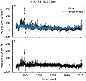
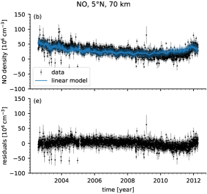
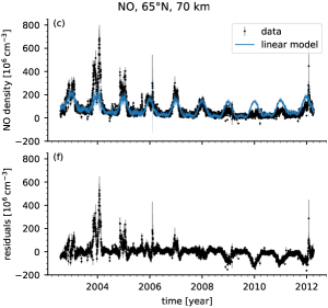
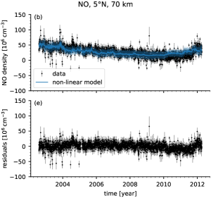
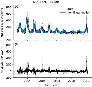
We demonstrate the parameter estimates using example time series at 70 km at 65\degreeS, 5\degreeN, and 65\degreeN. \chemNO shows different behaviour in these regions, showing the most variation with respect to the solar cycle and geomagnetic activity at high latitudes. In contrast, at low latitudes the geomagnetic influence should be reduced (Barth et al., 1988; Hendrickx et al., 2017; Kiviranta et al., 2018). We briefly only show the results for the linear model and point out some of its shortcomings. Thereafter we show the results from the non-linear model and continue to use that for further analysis of the coefficients.
4.1 Time series fits
The fitted densities of the linear model Eq. (1) compared to the data are shown in the upper panels of Fig 1 for the three example latitude bins (65\degreeS, 5\degreeN, 65\degreeN) at 70 km. The linear model works well at high southern and low latitudes. At high northern latitudes and to a lesser extent at high southern latitudes, the linear model captures the summer \chemNO variations well. However, the model underestimates the high values in the polar winter at active times (2004–2007) and overestimates the low winter values at quiet times (2009–2011).
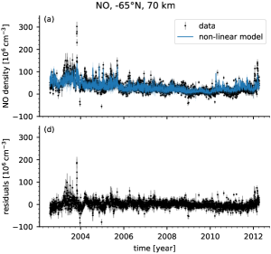
For the sample timeseries (65\degreeS, 5\degreeN, 65\degreeN at 70 km), the fits using the non-linear model Eq. (3) are shown in the upper panels of Fig 2. The non-linear model better captures both the summer \chemNO variations as well as the high values in the winter, especially at high northern latitudes. However, at times of high solar activity (2003–2006) and in particular at times of a strongly disturbed mesosphere (2004, 2006, 2012), the residuals are still significant. At high southern and low latitudes, the improvement over the linear model is less evident. At low latitudes, the \chemNO content is apparently mostly related to the eleven-year solar cycle and the particle influence is suppressed. Since this cycle is covered by the Lyman- index, both models perform similarly, but the non-linear version has one less parameter. In both regions the residuals show traces of seasonal variations that are not related to particle effects. The linear model appears to capture these variations better than the non-linear model. However, by objective measures including the number of model parameters111Past and recent research in model selection provides a number of choices on how to compare models objectively. The results are so-called information criteria which aim to provide a consistent way of how to compare models, most notably the “Akaike information criterion” (AIC; Akaike, 1974), the “Bayesian information criterion” or “Schwarz criterion” (BIC or SIC; Schwarz, 1978), the “deviance information criterion” (DIC; Spiegelhalter et al., 2002; Ando, 2011), or the “widely applicable information criterion” (WAIC; Watanabe, 2010; Vehtari et al., 2016). Alternatively, the “standardized mean squared error” (SMSE) or the “mean standardized log loss” (MSLL) (Rasmussen and Williams, 2006, chap. 2) give an impression of the quality of regression models with respect to each other. , the non-linear version fits the data better in all bins (not shown here). At high southern latitudes, the SCIAMACHY data are less densely sampled compared to high northern latitudes (see Bender et al., 2017b). In addition to the sampling differences, geomagnetic latitudes encompass a wider geographic range in the Southern Hemisphere (SH) than in the Northern Hemisphere (NH), and the AE index is derived from stations in the NH. Both effects can lower the \chemNO concentrations that SCIAMACHY observes in the SH, particularly at the winter maxima. The lifetime variation that improves the fit in the NH is thus less effective in the SH.
4.2 Parameter morphologies
Using the non-linear model, we show the latitude–altitude distributions of the medians of the sampled Lyman- and geomagnetic index coefficients in Fig. 3. The white regions indicate values outside of the 95% confidence region or whose sampled distribution has a skewness larger than 0.33. The MCMC method samples the parameter probability distributions. Since we require the geomagnetic index and constant lifetime parameters to be larger than zero (see Table 1), these sampled distributions are sometimes skewed towards zero even though the 95% credible region is still larger than zero. Excluding heavily skewed distributions avoids those cases because the “true” parameter is apparently zero.
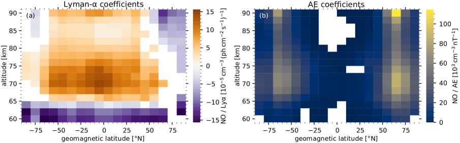
The Lyman- parameter distribution shows that its largest influence is at middle and low latitudes between 65 and 80 km. Another increase of the Lyman- coefficient is indicated at higher altitudes above 90 km. The penetration of Lyman- radiation decreases with decreasing altitude as a result of scattering and absorption by air molecules. On the other hand, the concentration of air decreases with altitude. At this stage we do not have an unambiguous explanation of this behaviour, but it may be related to reaction pathways as laid out by Pendleton et al. (1983), which would relate the \chemNO concentrations to the \chemCO_2 and \chemH_2O (or \chemOH, respectively) profiles. The Lyman- coefficients are all negative below 65 km. We also observe negative values at high northern latitude at all altitudes and at high southern latitudes above 85 km. These negative coefficients indicate that \chemNO photodissociation or conversion to other species outweighs its production via UV radiation in those places. The north–south asymmetry may be related to sampling and the difference in illumination with respect to geomagnetic latitudes; see Sect. 4.1.
The geomagnetic influence is largest at high latitudes between 50 and 75\degree above about 65 km. The AE coefficients peak at around 72 km and indicate a further increase above 90 km. This pattern of the geomagnetic influence matches the one found in Sinnhuber et al. (2016). Unfortunately both increased influences above 90 km in Lyman- and AE cannot be studied at higher latitudes due to a large a priori contribution to the data.
The latitude–altitude distributions of the lifetime parameters are shown in Fig. 4. All values shown are within the 95% confidence region. As for the coefficients above, we also exclude regions where the skewness was larger than 0.33.
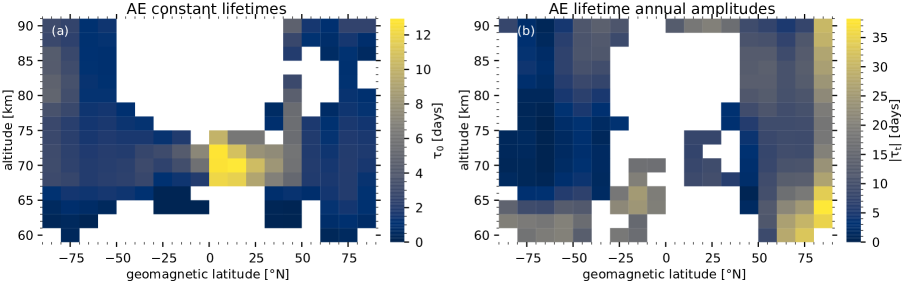
The constant part of the lifetime, , is below 2 days in most bins, except for exceptionally large values ( days) at low latitudes (0–20\degreeN) between 68 and 74 km. Although we constrained the lifetime with an exponential prior distribution, these large values apparently resulted in a better fit to the data. One explanation could be that because of the small geomagnetic influence (the AE coefficient is small in this region), the lifetime is more or less irrelevant. The amplitude of the annual variation (; see Eq. (6)) is largest at high latitudes in the Northern Hemisphere and at middle latitudes in the Southern Hemisphere. This difference could be linked to the geomagnetic latitudes which include a wider range of geographic latitudes in the Southern Hemisphere compared to the Northern Hemisphere. Therefore, the annual variation is less apparent in the Southern Hemisphere. The amplitude also increases with decreasing altitude below 75 km at middle and high latitudes and with increasing altitude above that. The increasing annual variation at low altitudes can be the result of transport processes that are not explicitly treated in our approach. Note that the term lifetime is not a pure (photo)chemical lifetime; rather it indicates how long the AE signal persists in the \chemNO densities. In that sense it combines the (photo)chemical lifetime with transport effects as discussed in Sinnhuber et al. (2016).
4.3 Parameter profiles
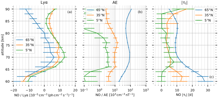
For three selected latitude bins in the Northern Hemisphere (5, 35, and 65\degreeN) we present profiles of the fitted parameters in Fig. 5. The solid line indicates the median, and the error bars indicate the 95% confidence region. As indicated in Fig. 3, the solar radiation influence is largest between 65 and 80 km. Its influence is also up to a factor of 2 larger at low and middle latitudes compared to high latitudes, where the coefficient only differs significantly from zero below 65 and above 82 km. Similarly, the geomagnetic impact decreases with decreasing latitude by 1 order of magnitude from high to middle latitudes and at least a further factor of 5 to lower latitudes. The largest impact is around 70–72 km and possibly above 90 km at high latitudes and is approximately constant between 66 and 76 km at middle and low latitudes. Note that the scale in Fig. 5b is logarithmic. The lifetime variation shows that at high latitudes, geomagnetically affected \chemNO persists longer during winter (the phase is close to zero for all altitudes at 65\degreeN, not shown here). It persists up to 10 days longer between 85 and 70 km and increasingly longer below, reaching 28 days at 60 km.
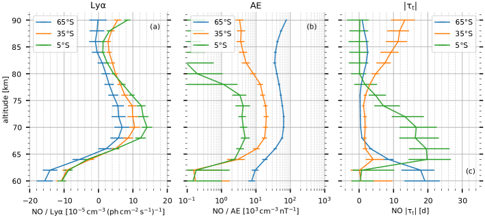
For the same latitude bins in the Southern Hemisphere (5\degreeS, 35\degreeS, and 65\degreeS) we present profiles of the fitted parameters in Fig. 6. Similar to the coefficients in the Northern Hemisphere (see Fig. 5), the solar radiation influence is largest between 65 km and 80 km and also up to a factor of two larger at low and middle latitudes compared to high latitudes. However, the Lyman- coefficients at 65\degreeS are significant below 82 km. Also the geomagnetic AE coefficients show a similar pattern in the Southern Hemisphere compared to the Northern Hemisphere, decreasing by orders of magnitude from high to low latitudes. Note that the AE coefficients at high latitudes are slightly lower than in the Northern Hemisphere, whereas the coefficients at middle and low latitudes are slightly larger. This slight asymmetry was also found in the study by Sinnhuber et al. (2016) and may be related to AE being derived solely from stations in the Northern Hemisphere (Mandea and Korte, 2011). With respect to latitude, the annual variation of the lifetime seems to be reversed compared to the Northern Hemisphere, with almost no variation at high latitudes and longer persisting \chemNO at low latitudes. A faster descent in the southern polar vortex may be responsible for the short lifetime at high southern latitudes. Another reason may be the mixture of air from inside and outside of the polar vertex when averaging along geomagnetic latitudes since the 65\degreeS geomagnetic latitude band includes geographic locations from about 45\degreeS to 85\degreeS. A third possibility may be the exclusion of the Southern Atlantic Anomaly from the retrieval (Bender et al., 2013, 2017b) where presumably the particle-induced impact on \chemNO is largest.
4.4 Discussion
The distribution of the parameters confirms our understanding of the processes producing \chemNO in the mesosphere to a large extent. The Lyman- coefficients are related to radiative processes such as production by UV or soft X-rays, either directly or via intermediary of photoelectrons. The photons are not influenced by Earth’s magnetic field, and the influence of these processes is largest at low latitudes and decreases towards higher latitudes. We observe negative Lyman- coefficients below 65 km at all latitudes and at high northern latitudes above 80 km. These negative Lyman- coefficients indicate that at high solar activity, photodissociation by nm photons, photoionization by nm photons, or collisional loss and conversion to other species outweigh the production from higher energy photons ( nm). At high southern latitudes these negative Lyman- coefficients are not as pronounced as at high northern latitudes. As mentioned in Sect. 4.2, this north–south asymmetry may be related to sampling and the difference in illumination with respect to geomagnetic latitudes, see also Sect. 4.1.
The AE coefficients are largest at auroral latitudes as expected for the particle nature of the associated \chemNO production. The AE coefficient can be considered an effective production rate modulated by all short-term ( day) processes. To roughly estimate this production rate, we divided the coefficient of the (daily) AE by 86400 s which follows the approach in Sinnhuber et al. (2016). We find a maximum production rate of about 1 cm-3 nT-1 s-1 around 70–72 km. This production rate also agrees with the one estimated by Sinnhuber et al. (2016) by a superposed epoch analysis of summertime \chemNO. Comparing the \chemNO production to the ionization rates from Verronen et al. (2013) from 1 to 3 January 2005 (assuming approximately 1 \chemNO molecule per ion pair), our model overestimates the ionization derived from AE on these days. The AE values of 105, 355, and 435 nT translate to 105, 355, and 435 \chemNO molecules cm-3 s-1, about 4 times larger than would be estimated from the ionization rates in Verronen et al. (2013) but agreeing with Sinnhuber et al. (2016). The factor of 4 may be related to the slightly different locations, around 60\degreeN (Verronen et al., 2013) compared to around 65\degreeN here and in Sinnhuber et al. (2016), in which the ionization rates may be higher.
The associated constant part of the lifetime ranges from around 1 to around 4 days, except for large at low latitudes around 70 km. As already discussed in Sect. 4.2, these large lifetimes may be a side effect of the small geomagnetic coefficients and more or less arbitrary. The magnitude is similar to what was found in the study by Sinnhuber et al. (2016) using only the summer data.
The annual variation of the lifetime is largest at high northern latitudes with a nearly constant amplitude of 10 days between 70 and 85 km. An empirical lifetime of 10 days in winter was used by Sinnhuber et al. (2016) to extend the \chemNO predicted by the summer analysis to the larger values in winter. Here we could confirm that 10 days is a good approximation of the \chemNO lifetime in winter, but it varies with altitude. The altitude distribution agrees with the increasing photochemical lifetime at large solar zenith angles (Sinnhuber et al., 2016, Fig. 7b). The larger values in our study are similarly related to transport and mixing effects which alter the observed lifetime. The small variation of the lifetime at high southern latitudes could be a sampling issue because SCIAMACHY only observes small variations there in winter (see Figs. 1 and 2). Note that the results (in particular the large annual variation) in the northernmost latitude bin should be taken with caution because this bin is sparsely sampled by SCIAMACHY, and the large winter \chemNO concentrations are actually absent from the data.
We propose an empirical model to estimate the \chemNO density in the mesosphere (60–90 km) derived from measurements from SCIAMACHY nominal-mode limb scans. Our model calculates \chemNO number densities for geomagnetic latitudes using the solar Lyman- index and the geomagnetic AE index. Two approaches were tested, a linear approach containing annual and semi-annual harmonics and a non-linear version using a finite and variable lifetime for the geomagnetically induced variations. From our proposed models, the linear variant only describes part of the \chemNO variations. It can describe the summer variations but underestimates the large number densities during winter. The non-linear version derived from the SCIAMACHY \chemNO data describes both variations using an annually varying finite lifetime for the particle-induced \chemNO. However, in cases of dynamic disturbances of the mesosphere, for example in early 2004 or in early 2006, the indirectly enhanced \chemNO (see, for example, Randall et al., 2007) is not captured by the model. These remaining variations are treated as statistical noise.
Sinnhuber et al. (2016) use a superposed epoch analysis limited to the polar summer to model the \chemNO data. Here we extend that analysis to use all available SCIAMACHY nominal-mode \chemNO data for all seasons. However, during summer the present results show comparable \chemNO production per AE unit and similar lifetimes to the Sinnhuber et al. (2016) study.
The parameter distributions indicate in which regions the different processes are significant. We find that these distributions match our current understanding of the processes producing and depleting \chemNO in the mesosphere (Funke et al., 2014a, b, 2016; Sinnhuber et al., 2016; Hendrickx et al., 2017; Kiviranta et al., 2018). In particular, the influence of Lyman- (or solar UV radiation in general) is largest at low and middle latitudes, which is explained by the direct production of \chemNO via solar UV or soft X-ray radiation (Barth et al., 1988, 2003). The geomagnetic influence is largest at high latitudes and is best explained by the production from charged particles that enter the atmosphere in the polar regions along the magnetic field.
A potential improvement would be to use actual measurements of precipitating particles instead of the AE index. Using measured fluxes could help to confirm our current understanding of how those fluxes relate to ionization (Turunen et al., 2009; Verronen et al., 2013) and subsequent \chemNO production (Sinnhuber et al., 2016). Furthermore, including dynamical transport, as for example in Funke et al. (2016), could improve our knowledge of the combined direct and indirect \chemNO production in the mesosphere.
SB developed the model, prepared and performed the data analysis and set up the manuscript, MS provided input on the model and the idea of a variable \chemNO lifetime. JPB and PJE contributed to the discussion and use of language. All authors contributed to the interpretation and discussion of the method and the results as well as to the writing of the paper.
The SCIAMACHY \chemNO data set used in this study is available at https://zenodo.org/record/1009078 (Bender et al., 2017a). The python code to prepare the data (daily zonal averaging) and to perform the analysis is available at https://zenodo.org/record/1401370 (Bender, 2018a) or at https://github.com/st-bender/sciapy. The daily zonal mean \chemNO data and the sampled parameter distributions are available at https://zenodo.org/record/1342701 (Bender, 2018b). The solar Lyman- index data were downloaded from http://lasp.colorado.edu/lisird/data/composite_lyman_alpha/, the AE index data were downloaded from http://wdc.kugi.kyoto-u.ac.jp/aedir/, and the daily mean values used in this study are available within the aforementioned data set.
Acknowledgements.
S.B. and M.S. thank the Helmholtz-society for funding part of this project under the grant number VH-NG-624. S.B. and P.J.E. acknowledge support from the Birkeland Center for Space Sciences (BCSS), supported by the Research Council of Norway under the grant number 223252/F50. The SCIAMACHY project was a national contribution to the ESA Envisat, funded by German Aerospace (DLR), the Dutch Space Agency, SNO, and the Belgium ministry. The University of Bremen as Principal Investigator has led the scientific support and development of the SCIAMACHY instrument as well as the scientific exploitation of its data products. This work was performed on the Abel Cluster, owned by the University of Oslo and Uninett/Sigma2, and operated by the Department for Research Computing at USIT, the University of Oslo IT-department. http://www.hpc.uio.no/References
- Akaike (1974) Akaike, H.: A new look at the statistical model identification, IEEE Transactions on Automatic Control, 19, 716–723, 10.1109/tac.1974.1100705, 1974.
- Ando (2011) Ando, T.: Predictive Bayesian Model Selection, American Journal of Mathematical and Management Sciences, 31, 13–38, 10.1080/01966324.2011.10737798, 2011.
- Bailey et al. (2002) Bailey, S. M., Barth, C. A., and Solomon, S. C.: A model of nitric oxide in the lower thermosphere, J. Geophys. Res. Space Phys., 107, 1205, 10.1029/2001JA000258, 2002.
- Baldwin and Dunkerton (2001) Baldwin, M. P. and Dunkerton, T. J.: Stratospheric Harbingers of Anomalous Weather Regimes, Science, 294, 581–584, 10.1126/science.1063315, 2001.
- Barth (1992) Barth, C. A.: Nitric oxide in the lower thermosphere, Planet. Space Sci., 40, 315–336, 10.1016/0032-0633(92)90067-x, 1992.
- Barth (1995) Barth, C. A.: Nitric Oxide in the Lower Thermosphere, in: The Upper Mesosphere and Lower Thermosphere: A Review of Experiment and Theory, edited by Johnson, R. M. and Killeen, T. L., pp. 225–233, American Geophysical Union, 10.1029/gm087p0225, 1995.
- Barth (2010) Barth, C. A.: Joule heating and nitric oxide in the thermosphere, 2, J. Geophys. Res. Space Phys., 115, A10 305, 10.1029/2010ja015565, 2010.
- Barth et al. (1988) Barth, C. A., Tobiska, W. K., Siskind, D. E., and Cleary, D. D.: Solar-terrestrial coupling: Low-latitude thermospheric nitric oxide, Geophys. Res. Lett., 15, 92–94, 10.1029/gl015i001p00092, 1988.
- Barth et al. (2003) Barth, C. A., Mankoff, K. D., Bailey, S. M., and Solomon, S. C.: Global observations of nitric oxide in the thermosphere, J. Geophys. Res. Space Phys., 108, 1027, 10.1029/2002JA009458, 2003.
- Barth et al. (2009) Barth, C. A., Lu, G., and Roble, R. G.: Joule heating and nitric oxide in the thermosphere, J. Geophys. Res. Space Phys., 114, A05 301, 10.1029/2008ja013765, 2009.
- Bender (2018a) Bender, S.: st-bender/sciapy: Version 0.0.5 [source code], 10.5281/zenodo.1401370, URL https://zenodo.org/record/1401370, 2018a.
- Bender (2018b) Bender, S.: SCIAMACHY NO regression fit MCMC samples [data set], 10.5281/zenodo.1342701, URL https://zenodo.org/record/1342701, 2018b.
- Bender et al. (2013) Bender, S., Sinnhuber, M., Burrows, J. P., Langowski, M., Funke, B., and López-Puertas, M.: Retrieval of nitric oxide in the mesosphere and lower thermosphere from SCIAMACHY limb spectra, Atmos. Meas. Tech., 6, 2521–2531, 10.5194/amt-6-2521-2013, URL http://www.atmos-meas-tech.net/6/2521/2013/, 2013.
- Bender et al. (2017a) Bender, S., Sinnhuber, M., Burrows, J. P., and Langowski, M.: Nitric oxide (NO) data set (60–160 km) from SCIAMACHY nominal limb scans, 10.5281/zenodo.804371, URL https://doi.org/10.5281/zenodo.804371, 2017a.
- Bender et al. (2017b) Bender, S., Sinnhuber, M., Langowski, M., and Burrows, J. P.: Retrieval of nitric oxide in the mesosphere from SCIAMACHY nominal limb spectra, Atmos. Meas. Tech., 10, 209–220, 10.5194/amt-10-209-2017, URL https://www.atmos-meas-tech.net/10/209/2017/, 2017b.
- Bermejo-Pantaleón et al. (2011) Bermejo-Pantaleón, D., Funke, B., López-Puertas, M., García-Comas, M., Stiller, G. P., von Clarmann, T., Linden, A., Grabowski, U., Höpfner, M., Kiefer, M., Glatthor, N., Kellmann, S., and Lu, G.: Global observations of thermospheric temperature and nitric oxide from MIPAS spectra at 5.3 µm, J. Geophys. Res. Space Phys., 116, A10 313, 10.1029/2011JA016752, 2011.
- Bovensmann et al. (1999) Bovensmann, H., Burrows, J. P., Buchwitz, M., Frerick, J., Noël, S., Rozanov, V. V., Chance, K. V., and Goede, A. P. H.: SCIAMACHY: Mission Objectives and Measurement Modes, J. Atmos. Sci., 56, 127–150, 10.1175/1520-0469(1999)056<0127:SMOAMM>2.0.CO;2, 1999.
- Burrows et al. (1995) Burrows, J. P., Hölzle, E., Goede, A. P. H., Visser, H., and Fricke, W.: SCIAMACHY – scanning imaging absorption spectrometer for atmospheric chartography, Acta Astronaut., 35, 445–451, 10.1016/0094-5765(94)00278-T, URL http://www.sciencedirect.com/science/article/pii/009457659400278T, 1995.
- Crutzen (1970) Crutzen, P. J.: The influence of nitrogen oxides on the atmospheric ozone content, Quart. J. Roy. Meteor. Soc., 96, 320–325, 10.1002/qj.49709640815, 1970.
- Davis and Sugiura (1966) Davis, T. N. and Sugiura, M.: Auroral electrojet activity index AE and its universal time variations, J. Geophys. Res., 71, 785–801, 10.1029/jz071i003p00785, 1966.
- Foreman-Mackey et al. (2013) Foreman-Mackey, D., Hogg, D. W., Lang, D., and Goodman, J.: emcee: The MCMC Hammer, Publ. Astron. Soc. Pac., 125, 306–313, 10.1086/670067, 2013.
- Foreman-Mackey et al. (2017) Foreman-Mackey, D., Agol, E., Angus, R., and Ambikasaran, S.: Fast and scalable Gaussian process modeling with applications to astronomical time series, The Astronomical Journal, 154, 220, 10.3847/1538-3881/aa9332, URL https://arxiv.org/abs/1703.09710, 2017.
- Foreman-Mackey et al. (2017) Foreman-Mackey, D., Agol, E., Angus, R., Brewer, B. J., Austin, P., Farr, W. M., Guillochon, J., Czekala, I., and Casey, A.: dfm/celerite: celerite v0.3.0, 10.5281/zenodo.1048287, 2017.
- Frost et al. (1956) Frost, D. C., McDowell, C. A., and Bawn, C. E. H.: The dissociation energy of the nitrogen molecule, Proceedings of the Royal Society of London. Series A. Mathematical and Physical Sciences, 236, 278–284, 10.1098/rspa.1956.0135, 1956.
- Funke et al. (2001) Funke, B., López-Puertas, M., Stiller, G., v. Clarmann, T., and Höpfner, M.: A new non-LTE retrieval method for atmospheric parameters from mipas-envisat emission spectra, Adv. Space Res., 27, 1099–1104, 10.1016/S0273-1177(01)00169-7, URL http://www.sciencedirect.com/science/article/pii/S0273117701001697, 2001.
- Funke et al. (2005a) Funke, B., López-Puertas, M., Gil-López, S., von Clarmann, T., Stiller, G. P., Fischer, H., and Kellmann, S.: Downward transport of upper atmospheric NOx into the polar stratosphere and lower mesosphere during the Antarctic 2003 and Arctic 2002/2003 winters, J. Geophys. Res. Atmos., 110, D24 308, 10.1029/2005JD006463, 2005a.
- Funke et al. (2005b) Funke, B., López-Puertas, M., von Clarmann, T., Stiller, G. P., Fischer, H., Glatthor, N., Grabowski, U., Höpfner, M., Kellmann, S., Kiefer, M., Linden, A., Mengistu Tsidu, G., Milz, M., Steck, T., and Wang, D. Y.: Retrieval of stratospheric NOx from 5.3 and 6.2 µm nonlocal thermodynamic equilibrium emissions measured by Michelson Interferometer for Passive Atmospheric Sounding (MIPAS) on Envisat, J. Geophys. Res. Atmos., 110, D09 302, 10.1029/2004JD005225, 2005b.
- Funke et al. (2008a) Funke, B., García-Comas, M., López-Puertas, M., Glatthor, N., Stiller, G. P., von Clarmann, T., Semeniuk, K., and McConnell, J. C.: Enhancement of N2O during the October–November 2003 solar proton events, Atmos. Chem. Phys., 8, 3805–3815, 10.5194/acp-8-3805-2008, 2008a.
- Funke et al. (2008b) Funke, B., López-Puertas, M., Garcia-Comas, M., Stiller, G. P., von Clarmann, T., and Glatthor, N.: Mesospheric N2O enhancements as observed by MIPAS on Envisat during the polar winters in 2002–2004, Atmos. Chem. Phys., 8, 5787–5800, 10.5194/acp-8-5787-2008, 2008b.
- Funke et al. (2012) Funke, B., López-Puertas, M., García-Comas, M., Kaufmann, M., Höpfner, M., and Stiller, G.: GRANADA: A Generic RAdiative traNsfer AnD non-LTE population algorithm, J. Quant. Spectrosc. Radiat. Transfer, 113, 1771–1817, 10.1016/j.jqsrt.2012.05.001, URL http://www.sciencedirect.com/science/article/pii/S0022407312002427, 2012.
- Funke et al. (2014a) Funke, B., López-Puertas, M., Holt, L., Randall, C. E., Stiller, G. P., and von Clarmann, T.: Hemispheric distributions and interannual variability of NOy produced by energetic particle precipitation in 2002-2012, J. Geophys. Res. Atmos., 119, 13,565–13,582, 10.1002/2014jd022423, 2014a.
- Funke et al. (2014b) Funke, B., López-Puertas, M., Stiller, G. P., and von Clarmann, T.: Mesospheric and stratospheric NOy produced by energetic particle precipitation during 2002–2012, J. Geophys. Res. Atmos., 119, 4429–4446, 10.1002/2013JD021404, 2014b.
- Funke et al. (2016) Funke, B., López-Puertas, M., Stiller, G. P., Versick, S., and von Clarmann, T.: A semi-empirical model for mesospheric and stratospheric NOy produced by energetic particle precipitation, Atmos. Chem. Phys., 16, 8667–8693, 10.5194/acp-16-8667-2016, URL https://www.atmos-chem-phys.net/16/8667/2016/, 2016.
- Funke et al. (2017) Funke, B., Ball, W., Bender, S., Gardini, A., Harvey, V. L., Lambert, A., López-Puertas, M., Marsh, D. R., Meraner, K., Nieder, H., Päivärinta, S.-M., Pérot, K., Randall, C. E., Reddmann, T., Rozanov, E., Schmidt, H., Seppälä, A., Sinnhuber, M., Sukhodolov, T., Stiller, G. P., Tsvetkova, N. D., Verronen, P. T., Versick, S., von Clarmann, T., Walker, K. A., and Yushkov, V.: HEPPA-II model–measurement intercomparison project: EPP indirect effects during the dynamically perturbed NH winter 2008–2009, Atmos. Chem. Phys., 17, 3573–3604, 10.5194/acp-17-3573-2017, URL http://www.atmos-chem-phys.net/17/3573/2017/, 2017.
- Heays et al. (2017) Heays, A. N., Bosman, A. D., and van Dishoeck, E. F.: Photodissociation and photoionisation of atoms and molecules of astrophysical interest, Astronomy & Astrophysics, 602, A105, 10.1051/0004-6361/201628742, 2017.
- Hendrickx et al. (2015) Hendrickx, K., Megner, L., Gumbel, J., Siskind, D. E., Orsolini, Y. J., Tyssøy, H. N., and Hervig, M.: Observation of 27 day solar cycles in the production and mesospheric descent of EPP-produced NO, J. Geophys. Res. Space Phys., 120, 8978–8988, 10.1002/2015JA021441, 2015JA021441, 2015.
- Hendrickx et al. (2017) Hendrickx, K., Megner, L., Marsh, D. R., Gumbel, J., Strandberg, R., and Martinsson, F.: Relative Importance of Nitric Oxide Physical Drivers in the Lower Thermosphere, Geophys. Res. Lett., 44, 10,081–10,087, 10.1002/2017gl074786, URL http://onlinelibrary.wiley.com/doi/10.1002/2017GL074786/full, 2017.
- Hendrickx et al. (2018) Hendrickx, K., Megner, L., Marsh, D. R., and Smith-Johnsen, C.: Production and transport mechanisms of NO in observations and models, Atmos. Chem. Phys. Discuss., 2018, 1–24, 10.5194/acp-2017-1188, URL https://www.atmos-chem-phys-discuss.net/acp-2017-1188/, 2018.
- Hendrie (1954) Hendrie, J. M.: Dissociation Energy of N2, The Journal of Chemical Physics, 22, 1503–1507, 10.1063/1.1740449, 1954.
- Kiviranta et al. (2018) Kiviranta, J., Pérot, K., Eriksson, P., and Murtagh, D.: An empirical model of nitric oxide in the upper mesosphere and lower thermosphere based on 12 years of Odin SMR measurements, Atmos. Chem. Phys., 18, 13 393–13 410, 10.5194/acp-18-13393-2018, 2018.
- Kockarts (1980) Kockarts, G.: Nitric oxide cooling in the terrestrial thermosphere, Geophys. Res. Lett., 7, 137–140, 10.1029/gl007i002p00137, 1980.
- MacKay (2003) MacKay, D.: Information Theory, Inference and Learning Algorithms, Cambridge University Press, URL http://www.inference.org.uk/mackay/itila/book.html, 2003.
- Mandea and Korte (2011) Mandea, M. and Korte, M., eds.: Geomagnetic Observations and Models, vol. 5 of IAGA Special Sopron Book Series, 10.1007/978-90-481-9858-0, 2011.
- Maric and Burrows (1992) Maric, D. and Burrows, J.: Formation of N2O in the photolysis/photoexcitation of NO, NO2 and air, J. Photochem. Photobiol., A, 66, 291–312, 10.1016/1010-6030(92)80002-d, 1992.
- Marsh et al. (2004) Marsh, D. R., Solomon, S. C., and Reynolds, A. E.: Empirical model of nitric oxide in the lower thermosphere, J. Geophys. Res. Space Phys., 109, A07 301, 10.1029/2003JA010199, 2004.
- Matérn (1960) Matérn, B.: Spatial Variation: Stachastic Models and Their Application to Some Problems in Forest Surveys and Other Sampling Investigations, vol. 36 of Lecture Notes in Statistics, Statens skogsforskningsinstitut, Springer-Verlag New York, 2 edn., 10.1007/978-1-4615-7892-5, originally published by the Swedish National Institute for Forestry Research, 1960, 1960.
- Matthes et al. (2017) Matthes, K., Funke, B., Andersson, M. E., Barnard, L., Beer, J., Charbonneau, P., Clilverd, M. A., de Wit, T. D., Haberreiter, M., Hendry, A., Jackman, C. H., Kretzschmar, M., Kruschke, T., Kunze, M., Langematz, U., Marsh, D. R., Maycock, A. C., Misios, S., Rodger, C. J., Scaife, A. A., Seppälä, A., Shangguan, M., Sinnhuber, M., Tourpali, K., Usoskin, I., van de Kamp, M., Verronen, P. T., and Versick, S.: Solar forcing for CMIP6 (v3.2), Geosci. Model Dev., 10, 2247–2302, 10.5194/gmd-10-2247-2017, URL http://www.geosci-model-dev.net/10/2247/2017/, 2017.
- Orsolini et al. (2017) Orsolini, Y. J., Limpasuvan, V., Pérot, K., Espy, P., Hibbins, R., Lossow, S., Raaholt Larsson, K., and Murtagh, D.: Modelling the descent of nitric oxide during the elevated stratopause event of January 2013, J. Atmos. Sol. Terr. Phys., 155, 50–61, 10.1016/j.jastp.2017.01.006, URL http://adsabs.harvard.edu/abs/2017JASTP.155...50O, 2017.
- Pendleton et al. (1983) Pendleton, W., Erman, P., Larsson, M., and Witt, G.: Observation of Strong NO Gamma-Band Radiation Induced in Thin N2-CO2and N2-H2O Targets by Electron Impact and Its Possible Relation to the Auroral Chemistry of NO, Phys. Scr., 28, 532–538, 10.1088/0031-8949/28/5/005, 1983.
- Pérot et al. (2014) Pérot, K., Urban, J., and Murtagh, D. P.: Unusually strong nitric oxide descent in the Arctic middle atmosphere in early 2013 as observed by Odin/SMR, Atmos. Chem. Phys., 14, 8009–8015, 10.5194/acp-14-8009-2014, URL http://www.atmos-chem-phys.net/14/8009/2014/, 2014.
- Randall et al. (2007) Randall, C. E., Harvey, V. L., Singleton, C. S., Bailey, S. M., Bernath, P. F., Codrescu, M., Nakajima, H., and Russell, J. M.: Energetic particle precipitation effects on the Southern Hemisphere stratosphere in 1992–2005, J. Geophys. Res. Atmos., 112, D08 308, 10.1029/2006JD007696, 2007.
- Randall et al. (2015) Randall, C. E., Harvey, V. L., Holt, L. A., Marsh, D. R., Kinnison, D., Funke, B., and Bernath, P. F.: Simulation of energetic particle precipitation effects during the 2003-2004 Arctic winter, J. Geophys. Res. Space Phys., 120, 5035–5048, 10.1002/2015ja021196, 2015.
- Rasmussen and Williams (2006) Rasmussen, C. E. and Williams, C. K. I.: Gaussian processes for machine learning, Adaptive Computation and Machine Learning, MIT Press, Cambridge, MA, URL http://www.gaussianprocess.org/gpml/chapters/, 2006.
- Roble (1995) Roble, R. G.: Energetics of the Mesosphere and Thermosphere, in: The Upper Mesosphere and Lower Thermosphere: A Review of Experiment and Theory, edited by Johnson, R. M. and Killeen, T. L., pp. 1–21, American Geophysical Union, 10.1029/gm087p0001, 1995.
- Schwarz (1978) Schwarz, G.: Estimating the Dimension of a Model, The Annals of Statistics, 6, 461–464, 10.1214/aos/1176344136, 1978.
- Semeniuk et al. (2008) Semeniuk, K., McConnell, J. C., Jin, J. J., Jarosz, J. R., Boone, C. D., and Bernath, P. F.: N2O production by high energy auroral electron precipitation, J. Geophys. Res. Atmos., 113, D16 302, 10.1029/2007jd009690, 2008.
- Sheese et al. (2016) Sheese, P. E., Walker, K. A., Boone, C. D., Bernath, P. F., and Funke, B.: Nitrous oxide in the atmosphere: First measurements of a lower thermospheric source, Geophys. Res. Lett., 43, 2866–2872, 10.1002/2015gl067353, 2016.
- Sinnhuber et al. (2011) Sinnhuber, M., Kazeminejad, S., and Wissing, J. M.: Interannual variation of NOx from the lower thermosphere to the upper stratosphere in the years 1991–2005, J. Geophys. Res. Space Phys., 116, A02 312, 10.1029/2010JA015825, 2011.
- Sinnhuber et al. (2012) Sinnhuber, M., Nieder, H., and Wieters, N.: Energetic Particle Precipitation and the Chemistry of the Mesosphere/Lower Thermosphere, Surv. Geophys., 33, 1281–1334, 10.1007/s10712-012-9201-3, 2012.
- Sinnhuber et al. (2016) Sinnhuber, M., Friederich, F., Bender, S., and Burrows, J. P.: The response of mesospheric NO to geomagnetic forcing in 2002–2012 as seen by SCIAMACHY, J. Geophys. Res. Space Phys., 121, 3603–3620, 10.1002/2015JA022284, URL http://onlinelibrary.wiley.com/doi/10.1002/2015JA022284/abstract, 2015JA022284, 2016.
- Sinnhuber et al. (2018) Sinnhuber, M., Berger, U., Funke, B., Nieder, H., Reddmann, T., Stiller, G., Versick, S., von Clarmann, T., and Wissing, J. M.: NOy production, ozone loss and changes in net radiative heating due to energetic particle precipitation in 2002–2010, Atmos. Chem. Phys., 18, 1115–1147, 10.5194/acp-18-1115-2018, URL https://www.atmos-chem-phys.net/18/1115/2018/acp-18-1115-2018.pdf, 2018.
- Siskind et al. (2000) Siskind, D. E., Nedoluha, G. E., Randall, C. E., Fromm, M., and Russell, J. M.: An assessment of southern hemisphere stratospheric NOx enhancements due to transport from the upper atmosphere, Geophys. Res. Lett., 27, 329–332, 10.1029/1999GL010940, 2000.
- Solomon et al. (1982) Solomon, S., Crutzen, P. J., and Roble, R. G.: Photochemical coupling between the thermosphere and the lower atmosphere: 1. Odd nitrogen from 50 to 120 km, J. Geophys. Res. Oceans, 87, 7206, 10.1029/jc087ic09p07206, 1982.
- Spiegelhalter et al. (2002) Spiegelhalter, D. J., Best, N. G., Carlin, B. P., and van der Linde, A.: Bayesian measures of model complexity and fit, Journal of the Royal Statistical Society: Series B (Statistical Methodology), 64, 583–639, 10.1111/1467-9868.00353, 2002.
- Thébault et al. (2015) Thébault, E., Finlay, C. C., Beggan, C. D., Alken, P., Aubert, J., Barrois, O., Bertrand, F., Bondar, T., Boness, A., Brocco, L., Canet, E., Chambodut, A., Chulliat, A., Coïsson, P., Civet, F., Du, A., Fournier, A., Fratter, I., Gillet, N., Hamilton, B., Hamoudi, M., Hulot, G., Jager, T., Korte, M., Kuang, W., Lalanne, X., Langlais, B., Léger, J.-M., Lesur, V., Lowes, F. J., Macmillan, S., Mandea, M., Manoj, C., Maus, S., Olsen, N., Petrov, V., Ridley, V., Rother, M., Sabaka, T. J., Saturnino, D., Schachtschneider, R., Sirol, O., Tangborn, A., Thomson, A., Tøffner-Clausen, L., Vigneron, P., Wardinski, I., and Zvereva, T.: International Geomagnetic Reference Field: the 12th generation, Earth, Planets and Space, 67, 79–98, 10.1186/s40623-015-0228-9, URL https://doi.org/10.1186/s40623-015-0228-9, 2015.
- Turunen et al. (2009) Turunen, E., Verronen, P. T., Seppälä, A., Rodger, C. J., Clilverd, M. A., Tamminen, J., Enell, C.-F., and Ulich, T.: Impact of different energies of precipitating particles on NOx generation in the middle and upper atmosphere during geomagnetic storms, J. Atmos. Sol. Terr. Phys., 71, 1176–1189, 10.1016/j.jastp.2008.07.005, 2009.
- Vehtari et al. (2016) Vehtari, A., Gelman, A., and Gabry, J.: Practical Bayesian model evaluation using leave-one-out cross-validation and WAIC, Statistics and Computing, 27, 1413–1432, 10.1007/s11222-016-9696-4, 2016.
- Verronen et al. (2013) Verronen, P. T., Andersson, M. E., Rodger, C. J., Clilverd, M. A., Wang, S., and Turunen, E.: Comparison of modeled and observed effects of radiation belt electron precipitation on mesospheric hydroxyl and ozone, J. Geophys. Res. Atmos., 118, 11,419–11,428, 10.1002/jgrd.50845, 2013.
- Watanabe (2010) Watanabe, S.: Asymptotic equivalence of Bayes cross validation and widely applicable information criterion in singular learning theory, Journal of Machine Learning Research (JMLR), 11, 3571–3594, URL http://www.jmlr.org/papers/v11/watanabe10a.html, 2010.