Towards the Right Kind of Fairness in AI
A guide on the different metrics. And the tool “Fairness Compass” to choose the best option for your project.

Abstract

Fairness is a concept of justice. Various definitions exist, some of them conflicting with each other. In the absence of an uniformly accepted notion of fairness, choosing the right kind for a specific situation has always been a central issue in human history. When it comes to implementing sustainable fairness in artificial intelligence systems, this old question plays a key role once again: How to identify the most appropriate fairness metric for a particular application? The answer is often a matter of context, and the best choice depends on ethical standards and legal requirements. Since ethics guidelines on this topic are kept rather general for now, we aim to provide more hands-on guidance with this document. Therefore, we first structure the complex landscape of existing fairness metrics and explain the different options by example. Furthermore, we propose the “Fairness Compass”, a tool which formalises the selection process and makes identifying the most appropriate fairness definition for a given system a simple, straightforward procedure. Because this process also allows to document the reasoning behind the respective decisions, we argue that this approach can help to build trust from the user through explaining and justifying the implemented fairness.

1 Introduction

The last few years have seen a number of tremendous breakthroughs in the field of artificial intelligence (AI). A significant part of this success is due to major advances in machine learning (ML), the data analytics technique behind AI. Machine learning does recognise correlations in large data sets. Due to its ability to process loads of information in short time, it can uncover statistical patterns in data that humans cannot spot. This gives access to new kind of insights from the data which allow improved data analysis and model predictions. Although not absolutely error-free, the results clearly outperform conventional approaches, and often even human experts. The areas of application are extensive and include medical diagnosis, university admission, loan allocation, recidivism prediction, recruitment, online advertisement, face recognition, language translation, recommendation engines, fraud detection, credit limits, pricing and false news detection.

The heavy dependence on data poses a new challenge though. The data used for training a machine learning algorithm are considered the ground truth. This means that during the learning phase, these data constitute the comprehensive representation of the real world which the algorithm seeks to approximate. If the training data includes any kind of unwanted bias, the resulting algorithm will incorporate and enforce it. Worse still, in the absence of robust explanations for the results, it is hardly possible for humans to recognise biased predictions of machine learning algorithms as such.

Unwanted bias may happen to be directed against sensitive subgroups, defined for instance by gender, ethnicity or age. As a consequence, people from one such group would be generally disadvantaged by the system. However, systematic unequal treatment of individuals from different sensitive groups is considered discrimination, and there is broad consensus in our society that making a distinction based on a personal characteristic which is usually not a matter of choice is unfair. Hence, anti-discrimination laws in plenty of legislations prohibit actions of this nature.

The traditional approach to fight discrimination in statistical models when using deterministic algorithms is known as “anti-classification”. This principle is firmly encoded in current legal standards and it simply rules to exclude any attribute which defines membership in a sensitive subgroup as feature from the data. For example, a user’s gender may not be collected and processed in many scenarios. However, since machine learning is backed by “big data” which contain highly correlated features that can serve as possible proxies for those sensitive attributes, this approach has been shown to be insufficient to avoid discrimination in AI systems [1].

Two main sources for undesired bias have been identified in the machine learning pipeline. First, if the training data are incorrect or not sufficiently representative in certain aspects, this fault may become the source of correlations which do not exist in this form in reality. In such a case, the machine learning algorithm may detect patterns which are in fact not meaningful. Second, the training data may indeed faithfully represent the real world, but the status quo does not appear ideal. Without correction, the machine learning algorithm would reproduce the current state and thus manifest an existing shortcoming. The objective is therefore to adjust for this bias in the resulting algorithm.

Whatever the source, plenty of mitigation techniques have been presented by researchers lately to deal with bias in data and make AI applications more fair. This is an encouraging development towards maintaining trust in AI and eventually overcoming some of the potentially biased human judgments which impair automatic decision-making. Besides the technical task of adjusting the algorithms or the data, an equally important philosophical question needs to be settled: what kind of fairness is the objective? Fairness is a concept of justice and a variety of definitions exist which sometimes conflict with each other. Hence, there is no uniformly accepted notion of fairness available. In fact, the most appropriate fairness definition depends on the use case and it is often a matter of legal requirements and ethical standards.

The purpose of this document is to assist AI stakeholders in settling for the desired ethical principles by questions and examples. Applying such a procedure will not only help to identify the best fairness definition for a given AI application, but it will also make the choice transparent and the implemented fairness more understandable for the end user.

In the remainder, we first introduce some mathematical basics which are useful to assess and compare the performance of machine learning algorithms. Second, we explain the problem of unwanted bias in data. Next, we present the most commonly used fairness definitions in research and explain the ethical principles they stand for. Afterwards, we illustrate by example how these fairness definitions may be mutually contradictory. Finally, we present the “Fairness Compass” which constitutes an actionable guide for AI stakeholders to translate ethical principles into fairness definitions.

2 Fundamentals

For better understanding of the following sections, we introduce here some fundamental knowledge about machine learning, and a few statistical measures commonly used to characterise its performance.

2.1 Machine Learning

Compared with traditional programming, the difference of machine learning is that the reasoning behind the algorithm’s decision-making is not defined by hard-coded rules which were explicitly programmed by a human, but it is rather learned by example data: Thousands, sometimes millions of parameters get optimised without human intervention to finally capture a generalised pattern of the data. The resulting model allows to make predictions on new, unseen data with high accuracy.

This approach can be used for two different kinds of problems: On the one hand for classification, where the task is to predict discrete classes such as categories, for example. On the other hand for regression, where the objective is to predict a continuous quantity, for instance a price. Throughout this document, we only consider classification tasks, and for the sake of simplicity, we focus on the binary case with two classes: positive (1) or negative (0). For model output we either consider those very class labels 0 and 1, or a score $S$ which corresponds to the probability for the sample to be positive.

To illustrate the concepts in this document, we introduce a sample scenario about fraud detection in insurance claims. This fictional setting will serve as a running example throughout the following sections. Verifying the legitimacy of an insurance claim is essential to prevent abuse. However, fraud investigations are labour intensive for the insurance company. In addition, for some types of insurance, many claims may occur at the same time – for example, due to natural disasters that affect entire regions. For policyholders, on the other hand, supplementary checks can be annoying, for example when they are asked to answer further questions or provide additional documents. Both parties are interested in a quick decision: The customers expect timely remedy, and the company tries to keep the effort low. Therefore, an AI system that speeds up such a task could prove very useful. Concretely, it should be able to reliably identify legitimate insurance claims in order to make prompt payment possible. Potentially fraudulent cases should also be reliably detected and flagged for further investigation.

In order to analyse the performance of a classifier, we compare the predicted output $\widehat{Y}$ with the true output value $Y$. In the claims data, the output value 1 stands for a fraudulent claim, while 0 represents a legitimate claim. Table 1 shows sample predictions for our running example. For better illustration, we also provide a graphical representation of the same results in Figure 1. The white dots correspond to the positive samples ($Y=1$), here actual fraudulent claims. The black dots represent negative samples ($Y=0$), actual legitimate claims in the present scenario. The big circle constitutes the boundary of the classifier: Dots within the circle have been predicted as positive/fraudulent ($\widehat{Y}=1$), dots outside the circle as negative/legitimate ($\widehat{Y}=0$). The different background colours further show where the classifier was right (green and dark grey), and where not (red and light grey).

$Y$	* #9 in 142&0	* #9 in 121&1
$\widehat{Y}$	* #9 in 130&0	* #9 in 112&1	* #9 in 19&1	* #9 in 112&0

Table 1: Tabular evaluation of the sample scenario: true output class $Y$ compared to predictions $\widehat{Y}$

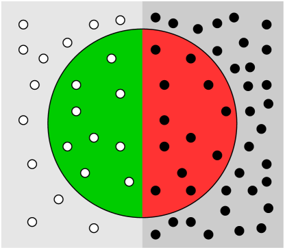
Figure 1: Graphical representation of the sample scenario. White dots represent positive samples, black ones negative samples. The big circle constitutes the classifier.

It is worth noting that in this oversimplified 2-dimensional example, drawing an ideal border which separates black and white dots and thus defining a perfect classifier would be obvious. In high-dimensional real world use cases, however, it is hardly possible to obtain a perfect classifier with error rates of zero; optimisation always remains a matter of trade-offs.

2.2 Statistical Measures

A so-called “confusion matrix” helps to visualise and compute statistical measures commonly used to inspect the performance of a machine learning model. The rows of the matrix represent the actual output classes, in our case 0 or 1. The columns represent the predicted output classes by the given classifier. The cells where the predicted class corresponds to the actual class contain the counts of the correctly classified instances. Wherever the classes differ, the classifier got it wrong and the numbers represent incorrectly classified samples.

		Predicted
		$\widehat{Y}$=1	$\widehat{Y}$=0
	$Y$=1	True positives (TP)	False negatives (FN)
True	$Y$=0	False positives (FP)	True negatives (TN)

Table 2: Schema of confusion matrix

On an abstract level, the figures in the cells are generally identified by the terms provided in Table 2. Taking the data from our running example in Table 1 as a basis, the related confusion matrix looks like Table 3. We notice that the given classifier correctly predicted 9 claims to be fraudulent and 30 claims to be legitimate. However, it also falsely predicted 12 claims to be legitimate, which were in fact fraudulent, and 12 claims to be fraudulent, which really were not.

		Predicted
		$\widehat{Y}$=1	$\widehat{Y}$=0
	$Y$=1	9	12
True	$Y$=0	12	30

Table 3: Confusion matrix for the sample data from Table 1

Revisiting the illustration in Figure 1, we further realise that the coloured segments in the schema correspond to the different cells in the confusion matrix: false negatives (light grey), true positives (green), false positives (red), and true negatives (dark grey).

From the confusion matrix we can extract plenty of interesting statistical measures. We describe those measures in the text and provide their formulas and graphical representations in Table 4.

Actual positives	$P=FN+TP$
Actual negatives	$N=FP+TN$
Base rate	$BR=\frac{P}{P+N}$
Positive rate	$PR=\frac{TP+FP}{P+N}$
Negative rate	$NR=\frac{TN+FN}{P+N}$
Accuracy	$ACC=\frac{TP+TN}{P+N}$
Misclassification rate	$MR=\frac{FN+FP}{P+N}$
True positive rate	$TPR=\frac{TP}{P}$
True negative rate	$TNR=\frac{TN}{N}$
False positive rate	$FPR=\frac{FP}{N}$
False negative rate	$FNR=\frac{FN}{P}$
False discovery rate	$FDR=\frac{FP}{TP+FP}$
Positive predictive value	$PPV=\frac{TP}{TP+FP}$
False omission rate	$FOR=\frac{FN}{TN+FN}$
Negative predictive value	$NPV=\frac{TN}{TN+FN}$

Table 4: Metrics derived from confusion matrix

First, we count the actual positives in the data set. This number is the sum of the true positives and the false negatives, which can be viewed as missed true positives. Likewise, the number of actual negatives is the sum of the true negatives and the false positives, which again can be viewed as missed true negatives. In our example, those figures represent the numbers of actual fraudulent claims and actual legitimate claims.

The (positive) base rate, sometimes also called the prevalence rate, represents the proportion of actual positives with respect to the entire data set. In our example, this rate describes the share of actual fraudulent claims in the data set.

The positive rate is the overall rate of positively classified instances, including both correct and incorrect decisions. The negative rate is the ratio of negative classification, again irrespective of whether the decisions were correct or incorrect. In our example, the positive rate is the rate of all claims suspected to be fraudulent, and the negative rate represents the rate of claims which are predicted to be legitimate.

Accuracy is the ratio of the correctly classified instances (positive and negative) of all decisions. In return, the misclassification rate is the ratio of the misclassified instances over all decisions. In our example, accuracy is the proportion of claims which were correctly classified, either as fraudulent or as legitimate. The misclassification rate refers to the failed classifications, the proportion of incorrect decisions taken by the classifier.

The true positive rate and the true negative rate describe the proportions of correctly classified positive and negative instances, respectively, of their actual occurrences. In the example, the true positive rate describes the share of all actual fraudulent claims which were detected as such. The true negative rate is the share of actual legitimate claims which were successfully discovered.

Directly linked, the false positive rate and the false negative rate describe the error rates. The false positive rate denotes the proportion of actual negatives which was falsely classified as positive. In the same way, the false negative rate describes the proportion of actual positives which was misclassified as negative. In our example, the false positive rate is the proportion of all actual legitimate claims which were falsely classified as fraudulent. On the other way around, the false negative rate is the proportion of all actual fraudulent claims which slipped through the system and were falsely classified as legitimate.

The false discovery rate describes the share of misclassified positive classifications of all positive predictions. So, it is about the proportion of positively classified instances which were falsely identified or discovered as such. On the contrary, the false omission rate describes the proportion of false negative predictions of all negative predictions. These instances, which are actually positive, were overlooked – they were mistakenly passed over or omitted. In our example, the false discovery rate is the error rate of all claims which were classified as fraudulent. The false omission rate describes the share of actually fraudulent claims of all claims which were classified as legitimate.

In a similar approach, but rather focusing on the correctly classified samples, the positive and the negative predictive values describe the ratio of samples which were correctly classified as positive or negative from all the positive or negative predictions. In the example, the positive predictive value is the proportion of correctly identified claims in all claims which were flagged as fraudulent. The negative predictive value is the proportion of correctly classified claims in all claims which were flagged as legitimate.

3 Problem of Bias

Up until here, we have analysed the data as one population and did not consider the possible existence of sensitive subgroups in the data. However, since decisions from machine learning algorithms often affect humans, many data sets contain sensitive subgroups by nature of the data. Such subgroups may for example be defined by gender, race or religion. The membership of an instance is usually identified by a sensitive attribute $A$. To analyse potential bias of a classifier, we split the results by this sensitive attribute into subgroups and investigate possible discrepancies among them. Any such deviation could be an indicator for discrimination against one sensitive group.

The idea of pursuing fairness on the basis of membership in one or several sensitive groups is called “group fairness” [2]. This approach is also adopted in anti-discrimination laws in many legislations with varying lists of sensitive attributes [3, 4]. In addition, another concept exists in research which tries to achieve “individual fairness” by aiming at similar treatment of similar individuals, taking any attribute into account [5]. In the scope of this document, we focus on group fairness, and to facilitate matters, we only consider two different sensitive subgroups. Therefore, we assume one sensitive binary attribute $A$ which can take the values 0 or 1, for instance representing the gender.

Unwanted bias is said to occur when the statistical measures described in the previous section significantly differ from one sensitive subgroup to another. Without any closer analysis on a per-subgroup basis, such a problem can go completely unnoticed. Please note that in order to “see” the groups in the data the sensitive information is obviously required to be available.

We now examine our running example on insurance fraud detection for unwanted bias. The output from the trained model remains unchanged, but this time we assume two sensitive subgroups in the data, specified by the sensitive attribute $A$. For instance, we split the data into men ($A$=0) and women ($A$=1). The separate confusion matrices for each subgroup in Table 5 enable us to compare the performance measures.

$A$=0		Predicted
		$\widehat{Y}$=1	$\widehat{Y}$=0	BR= round((7+7)/(7+7+6+22),2)
	$Y$=1	7	7	TPR= round((7)/(7+7),2)
True	$Y$=0	6	22	TNR= round((22)/(6+22),2)
		FDR= round((6)/(7+6),2)	FOR= round((7)/(7+22),2)
		PR=round((7+6)/(7+7+6+22),2)	NR= round((7+22)/(7+7+6+22),2)

(a) Men

$A$=1		Predicted
		$\widehat{Y}$=1	$\widehat{Y}$=0	BR= round((2+5)/(2+5+6+8),2)
	$Y$=1	2	5	TPR= round((2)/(2+5),2)
True	$Y$=0	6	8	TNR= round((8)/(6+8),2)
		FDR= round((6)/(2+6),2)	FOR= round((5)/(5+8),2)
		PR=round((2+6)/(2+5+6+8),2)	NR= round((5+8)/(2+5+6+8),2)

(b) Women

Table 5: Separate confusion matrices for sensitive subgroups

We notice that the base rates (BR) are identical in both subgroups which means in this example that men and women are equally likely to file a fraudulent (or a legitimate) claim. However, the true negative rate (TNR) for men is 0.79, while for women it is 0.57. This means 79% of the valid claims filed by men get correctly classified as legitimate, while for women that’s the case for only 57% of the same type of claims. On the other hand, the false omission rate for men is 24% and for women it is 38%. So, fraudulent claims filed by women have a higher chance to remain undetected than fraudulent claims filed by men.

4 Available Fairness Definitions

The problem of biased AI has attracted attention only recently, but the research community has already produced several fairness definitions to measure unwanted bias in outputs of machine learning models as described in the previous section. Additionally, plenty of mitigation methods have been proposed to ensure the kind of fairness they represent. For more details on the different mitigation approaches we refer the interested reader to survey papers on the subject as a starting point [1, 2]. In this document, we focus on the definitions of fairness and their impact on the results in real world scenarios.

In the following, we present the most commonly used definitions for group fairness and explain their characteristics by example. Since all notions relate to one of three fundamental conditions of statistical independence which are commonly known as independence, sufficiency, and separation, we segment the definitions by those categories [6].

4.1 Independence

Statistically, fairness definitions satisfy independence if the sensitive attribute $A$ is unconditionally independent of the prediction $\widehat{Y}$. Practically, this means that when considering all predictions made, the share of positive and negative decisions is proportionally equal among the two sensitive subgroups. On an individual level, this means that the likelihood of being classified as one of the classes is equal for two individuals with different sensitive attributes.

4.1.1 Demographic Parity

The goal of demographic parity is that the favourable outcome should be assigned to each subgroup of a sensitive class at equal rates [5].

In our running sample scenario, this objective translates to equal rates of negative predictions (=classifications as legitimate) for any claims submitted by men or women. In statistical terms, the negative rates (NR) of both subgroups should be identical. However, for the distributions above, NR=0.42 for men and NR=0.67 for women. We notice a gap of 25 percent points for the favourable outcome between the two sensitive subgroups.

The confusion matrices in Table 6 show possible results for a new model which was optimised for demographic parity. The number of negative predictions has increased for men, the distribution for women remains unchanged. Both confusion matrices now feature a NR of 0.67. Therefore, demographic parity was successfully achieved. It is not surprising though that manipulating the distribution for men also changes true positive and true negative rates.

$A$=0		Predicted
		$\widehat{Y}$=1	$\widehat{Y}$=0	BR= round((3+9)/(3+9+9+15),2)
	$Y$=1	3	9	TPR= round((3)/(3+9),2)
True	$Y$=0	9	15	TNR= round((15)/(9+15),2)
		FDR= round((9)/(3+9),2)	FOR= round((9)/(9+15),2)
		PR=round((3+9)/(3+9+9+15),2)	NR= round((9+15)/(3+9+9+15),2)

(a) Men

$A$=1		Predicted
		$\widehat{Y}$=1	$\widehat{Y}$=0	BR= round((6+3)/(6+3+3+15),2)
	$Y$=1	6	3	TPR= round((6)/(6+3),2)
True	$Y$=0	3	15	TNR= round((15)/(3+15),2)
		FDR= round((3)/(6+3),2)	FOR= round((3)/(3+15),2)
		PR=round((6+3)/(6+3+3+15),2)	NR= round((3+15)/(6+3+3+15),2)

(b) Women

Table 6: Optimised for Demographic Parity

4.1.2 Conditional Statistical Parity

This definition extends demographic parity by allowing a set of legitimate factors to affect the prediction. The definition is satisfied if members in both subgroups have equal probabilities of being assigned to the favourable outcome while controlling for a set of legitimate attributes [7].

In our example, a person’s history of prior convictions for fraud could be a legitimate attribute affecting the probability for a claim to be investigated. In this case, an attribute which documents previous attempts of fraud could serve as explaining variable.

4.1.3 Equal Selection Parity

While demographic parity seeks to obtain equal rates of a positive outcome, proportional towards the group size, the objective of equal selection parity is to have equal absolute numbers of favourable outcomes across the groups, independent of their group sizes [8].

In the example about fraud detection, this fairness definition would be satisfied if the exact same number of cases were to be identified as legitimate from both groups, even when one group had filed more cases than the other.

4.2 Sufficiency

Fairness notions satisfy the statistical concept of sufficiency when the sensitive attribute $A$ is conditionally independent of the true output value $Y$ given the predicted output $\widehat{Y}$. In other words, when considering all positive and negative predictions, the share of correct decisions is equal for both sensitive subgroups. On the individual level this translates to equal chances for individuals with identical predictions but different sensitive attributes to have obtained the right label.

4.2.1 Conditional Use Accuracy Equality

This fairness definition conditions on the algorithm’s predicted outcome, not on the actual outcome [9]. In statistical terms this means that the positive predictive value (PPV) and the negative predictive value (NPV) across both groups should be equal.

In the context of our example, the objective of this fairness definition is that for the claims which were predicted as fraud, the proportion of correct predictions should be equal across all groups. Likewise, for the claims which were predicted as legitimate, the proportion of correct predictions should be the same.

4.2.2 Predictive Parity

Predictive parity is a relaxed version of conditional use accuracy equality which only conditions on the positive predicted outcome [10]. Hence, this fairness definition is already satisfied when only the positive predictive value (PPV) is equal for both groups.

4.2.3 Calibration

Calibration is similar to conditional use accuracy equality but instead of the binary output it conditions on the predicted probability score $S$. The objective is again to obtain equal positive and negative predictive values for all sensitive groups [11]. Such a form of calibration across subgroups corresponds to equal probabilities of correct (or incorrect) classification and can therefore be achieved by aligning false discovery and false omission rates.

In the context of our example, calibrating the predictions of the classifier would result in equal chances for men and women to get their legitimate claims investigated without cause or to have their fraudulent claims falsely approved.

The two confusion matrices in Table 7 show the results of the classifier after calibration. The distribution for men was adjusted to match the one for women, which was not modified. Due to the equal base rates in both distributions, this action has also aligned all other statistical measures.

$A$=0		Predicted
		$\widehat{Y}$=1	$\widehat{Y}$=0	BR= round((8+4)/(8+4+4+20),2)
	$Y$=1	8	4	TPR= round((8)/(8+4),2)
True	$Y$=0	4	20	TNR= round((20)/(4+20),2)
		FDR= round((4)/(8+4),2)	FOR= round((4)/(4+20),2)
		PR=round((8+4)/(8+4+4+20),2)	NR= round((4+20)/(8+4+4+20),2)

(a) Men

$A$=1		Predicted
		$\widehat{Y}$=1	$\widehat{Y}$=0	BR= round((6+3)/(6+3+3+15),2)
	$Y$=1	6	3	TPR= round((6)/(6+3),2)
True	$Y$=0	3	15	TNR= round((15)/(3+15),2)
		FDR= round((3)/(6+3),2)	FOR= round((3)/(3+15),2)
		PR=round((6+3)/(6+3+3+15),2)	NR= round((3+15)/(6+3+3+15),2)

(b) Women

Table 7: Optimised for Calibration

4.3 Separation

Fairness definitions satisfy the principle of separation if the sensitive attribute $A$ is conditionally independent of the predicted output $\widehat{Y}$ given the true output value $Y$. This means that among both classes, the proportions of correct predictions are equal per sensitive subgroup. On an individual basis, this condition ensures that two individuals who actually belong to the same class but have different sensitive attributes share the same chance to obtain a correct prediction.

4.3.1 Equalised Odds

Another fairness definition called equalised odds aims at equal true positive and true negative rates [12]. The reasoning behind this concept is that the probabilities of being correctly classified should be the same for everyone.

In our recurring example, pursuing equalised odds means that the chances for claims to be correctly classified as legitimate or fraudulent should be equal for men and women; the classifier should not be more or less accurate for one of the subgroups.

In Table 8, we show a possible outcome for our example after optimising for equalised odds. The results for men have been reshuffled to match the true positive and true negative rates of the women. Since the base rates are equal in both subgroups, all other statistical measures have been aligned, too, by this operation.

$A$=0		Predicted
		$\widehat{Y}$=1	$\widehat{Y}$=0	BR= round((8+4)/(8+4+4+20),2)
	$Y$=1	8	4	TPR= round((8)/(8+4),2)
True	$Y$=0	4	20	TNR= round((20)/(4+20),2)
		FDR= round((4)/(8+4),2)	FOR= round((4)/(4+20),2)
		PR=round((8+4)/(8+4+4+20),2)	NR= round((4+20)/(8+4+4+20),2)

(a) Men

$A$=1		Predicted
		$\widehat{Y}$=1	$\widehat{Y}$=0	BR= round((6+3)/(6+3+3+15),2)
	$Y$=1	6	3	TPR= round((6)/(6+3),2)
True	$Y$=0	3	15	TNR= round((15)/(3+15),2)
		FDR= round((3)/(6+3),2)	FOR= round((3)/(3+15),2)
		PR=round((6+3)/(6+3+3+15),2)	NR= round((3+15)/(6+3+3+15),2)

(b) Women

Table 8: Optimised for Equalised Odds

4.3.2 Equalised Opportunities

Optimising for equalised odds can be a difficult task with more complex, real data, therefore the fairness definition equalised opportunities was proposed as more practicable alternative [12]. In this relaxed version of equalised odds, only the error rates for the positive outcome are required to be equal.

In our example, equalised opportunities is achieved when men and women who filed fraudulent claims are exposed at same rates. For legitimate claims, the rates may differ.

4.3.3 Predictive Equality

Another relaxation of equalised odds is predictive equality. Here, only the error rates for the negative outcome are required to be equal [13].

In our example, predictive equality is satisfied when men and women can expect their legitimate claims to get classified as legitimate at equal rates. The error rates for fraudulent claims may differ between the subgroups for this fairness definition.

As before, the confusion matrix for women in Table 9 is unchanged. For men, the output was modified in order to harmonise the false positive rate among the subgroups. The error rates for the unfavourable outcome of being suspect of fraud still deviate depending on the gender.

$A$=0		Predicted
		$\widehat{Y}$=1	$\widehat{Y}$=0	BR= round((9+3)/(9+3+4+20),2)
	$Y$=1	9	3	TPR= round((9)/(9+3),2)
True	$Y$=0	4	20	TNR= round((20)/(4+20),2)
		FDR= round((4)/(9+4),2)	FOR= round((3)/(3+20),2)
		PR=round((9+4)/(9+3+4+20),2)	NR= round((3+20)/(9+3+4+20),2)

(a) Men

$A$=1		Predicted
		$\widehat{Y}$=1	$\widehat{Y}$=0	BR= round((6+3)/(6+3+3+15),2)
	$Y$=1	6	3	TPR= round((6)/(6+3),2)
True	$Y$=0	3	15	TNR= round((15)/(3+15),2)
		FDR= round((3)/(6+3),2)	FOR= round((3)/(3+15),2)
		PR=round((6+3)/(6+3+3+15),2)	NR= round((3+15)/(6+3+3+15),2)

(b) Women

Table 9: Optimised for Predictive Equality

4.3.4 Balance

All previous fairness notions which aim at satisfying separation took binary outputs as a basis. The balance definition uses the predicted probability score instead and compares the average score for both groups per class. This approach seeks to avoid steadily lower outcomes in one group, which might go unnoticed in the binary case, and instead achieve balanced scores for both groups. Depending on the objective it is possible to balance for the positive or negative class [14].

5 The Dilemma

Presented with all these different fairness definitions it would be convenient to obtain “complete fairness” – one ultimate solution which satisfies all kinds of fairness at the same time. However, there is mathematical tension across the different fairness definitions, and it has been shown that some of them are actually incompatible with each other in realistic scenarios [14, 15, 1]. In this case, optimising for one metric comes with discounts for another. Taking a closer look this seems obvious considering the links between the fairness definitions and the conditional relations within the confusion matrix: The formulas share some of the cell counts, and the cell counts themselves are related to each other (e.g. the sums across the rows, which represent the numbers of true observations, are fixed).

In public, especially the trade-off between calibration and equal false positive and false negative rates (equalised odds) was much discussed. The debate was initiated by a ML algorithm called the “Correctional Offender Management Profiling for Alternative Sanctions”, or COMPAS, which had been developed by the company Northpointe, Inc. The objective of the COMPAS algorithm was to generate an independent, data derived “risk score” for several forms of recidivism. This kind of algorithm is used in the criminal justice sector in the US to support the judge with particular decisions such as granting of bail or parole. The score is of informative character and the final decision is still up to the judge. In May 2016, the investigative journalism website ProPublica focused attention on possible racial biases in the COMPAS algorithm [16]. Its main argument was based on analysis of the data which showed that the results were biased. In particular, the false positive rate for people who were black was significantly higher compared to people who were white. As a result, black people were disproportionately often falsely attributed a high risk of recidivism. Northpointe, on the other hand, responded to the accusations by arguing that the algorithm effectively achieved predictive parity for both groups [17]. In a nutshell, this ensured that risk scores corresponded to probabilities of reoffending, irrespective of any skin colour.

From an objective point of view, it can be stated that both parties make valid and reasonable observations of the data. However, the heated public debate revealed that it is unavoidable to precisely define and communicate the desired fairness objective for an application. This decision usually involves arbitration and compromise. For example in the given scenario, calibration and equalised odds could only be mutually satisfied if one of the following conditions was met: Either the base rates of the sensitive subgroups are exactly identical. Or, the outcome classes are perfectly separable which would allow for creating an ideal classifier that achieves perfect accuracy. Unfortunately, both requirements are very unlikely in real world scenarios.

6 Fairness Compass

Based on the limitations explained in the previous section, we conclude that it is crucial to consciously identify the most appropriate fairness definition for every single use case. To support AI stakeholders with this task, we propose the “Fairness Compass”, a schema in form of a decision tree which simplifies the selection process. By settling for the desired ethical principles in a formalised way, this schema not only makes identifying the most appropriate fairness definition a straightforward procedure, but it also helps document the underpinning decisions which may serve as deeper explanations to the end user why a specific fairness objective was chosen for the given application.

In this section, we first explain the general intended usage and then deep dive into the key decision points. Finally, we provide some technical specifications and outline how we hope to see this project evolve.

6.1 Usage

Primarily, the tool consists of the decision tree in LABEL:fig:flow_chart which formalises the decision process. There are three different types of nodes: The diamonds symbolise decision points, the white boxes stand for actions and the grey boxes with round corners are the fairness definitions. The arrows which connect the nodes represent the possible choices. For increased usability, the schema is also available as interactive online tool. In this version, tooltips with extended information, examples and references facilitate navigating the tree. Furthermore, the interactive online tool can be used to document the decision-making process for a specific application. The decision path can be highlighted in the diagram and the reasoning behind each decision can be added in the form of tooltips. In this way, the tool not only serves the AI stakeholders for decision-making but also as means of communication with the users. Due to the general complexity of the topic and the need for context-dependent solutions, we argue that sharing details with the broader audience when specifying fairness for a given use case is the best way forward to maintain confidence in AI systems.

6.2 Key Decision Nodes

In the following, we present the major questions we have identified in order to distinguish between the available fairness definitions. We describe each of them and provide practical examples.

6.2.1 Policy

Fairness objectives can go beyond equal treatment of different groups or similar individuals. If the target is to bridge prevailing inequalities by boosting underprivileged groups, affirmative actions or quotas can be valid measures. Such a goal may stem from law, regulation or internal organisational guidelines. This approach rules out any possible causality between the sensitive attribute and the outcome. If the data tells a different story in terms of varying base rates across the subgroups, this is a strong commitment which leads to subordinating the algorithm’s accuracy to the policy’s overarching goal. In any case, this decision limits the options to fairness definitions which hold the statistical principle of independence (subsection 4.1).

For example, many universities aim to improve diversity by accepting more students from disadvantaged backgrounds. Such admission policies acknowledge an equally high academic potential of students from sensitive subgroups and considers their possibly lower level of education rather an injustice in society than a personal shortcoming.

6.2.2 Type of Representation

If the decision node about policies from the previous section was answered with yes, particular emphasis is placed on equal representation of the sensitive subgroups. In this case, two different types of representation exist: equal numbers, regardless of the sizes of the subgroups; or proportional equality.

Let’s assume a recruitment scenario, for example, where ten women and two men applied for a job. Inviting two women and two men for an interview would satisfy gender fairness based on equal numbers. For proportional equality, it would be necessary to invite five women and one man.

6.2.3 Base Rates

Provided there is no policy in place which determines further proceedings, the next crucial question to settle concerns the base rate. This measure was already briefly introduced and it constitutes the proportion of actual positives or actual negatives of the entire data set (recapped in Figure 6). Across subgroups, the base rate can be equal, or it can be different. In case of varying rates, it is necessary to decide if the fairness definition should reflect this discrepancy or not. The former is the case when it is legitimate to assume a causal relationship between the group membership and the base rate, and the fairness definition is supposed to take this into account. The latter would be appropriate if there is no rational reason per se to believe that the groups perform differently, and the origin of the different base rates is rather to be found in the data collection process or other data related reasons. Yet another reason to choose equal rates as a basis, even though the data suggest otherwise, is when the discrepancy is considered to originate from historical discrimination. If the fairness objective is meant to make up for such social injustice in the past, assuming equal base rates helps to push the underprivileged group.

In [18], this question is formalised as two opposing worldviews: The worldview what you see is what you get (WYSIWYG) assumes the absence of structural bias in the data. Accordingly, this view supposes that any statistical variation in different groups actually represents deviating base rates which should get explored. On the other hand, the worldview we’re all equal (WAE) presupposes equal base rates for all groups. Possible deviations are considered as unwanted structural bias that needs to get corrected.

If base rates are assumed or expected to be equal across subgroups, only fairness definitions which satisfy independence (subsection 4.1) remain eligible. Otherwise, if the implemented fairness is to reflect the different base rates, definitions which hold sufficiency or separation (subsections 4.2 and 4.3) are to be considered.

In a medical scenario, the base rates for women and men to suffer from diabetes are equal, while 99% of breast cancer occurs in women. A fair diagnostic application should acknowledge this discrepancy. In a college admission scenario, however, different base rates in admission exams across different ethnic groups could be attributed to unequal opportunities. If the declared objective of the fairness definition is to correct such social injustice, choosing equal base rates can be a suitable approach.

$BR=\frac{P}{P+N}$

Figure 6: Formula and graphical representation of the (positive) base rate

6.2.4 Ground Truth

Machine learning algorithms are trained by example. The assumption is that the labels of the training data represent the true output, they constitute the supposed ground truth. As the labels serve as reference to estimate the model’s accuracy, but also to satisfy a fairness metric when this one is conditioning on the label, the availability of a reliable ground truth makes a significant difference.

Depending on the scenario, the ground truth may not exist or it may exist but not be available. When the correct outcome can be observed, the ground truth exists, and when the labels result from objective measurements or describe indisputable facts, the truth is easily accessible. In other cases, the correct outcome may not be directly measurable, but it is still unambiguously observable by humans who can perform annotation tasks with sufficient diligence to produce reliable labels. Sometimes, the ground truth does not exist. In such a scenario, labels are only inferred and represent subjective human decisions based on experience, and they may contain human bias.

When the ground truth is not available, and it cannot be produced in a trustworthy way neither, it is not recommended to select fairness definitions which rely on the true output value as is the case for the separation principle (subsection 4.3). Under these conditions, it is rather advisable to choose from fairness definitions which satisfy independence (subsection 4.1) and do not condition on the training label.

In a medical scenario, it is possible to conclusively clarify if a tumour is benign or malignant by taking a biopsy and performing a laboratory examination. Hence, the ground truth is available. In an image recognition application which helps classify animals, humans can make training data of good quality available by manually labelling the different species. When predicting recidivism, the ground truth is not immediately available since a possible new criminal offence would take place in the future and may not even be caught.

6.2.5 Explaining Variables

The data may contain variables which are considered legitimate sources of discrepancy. If some kind of inequality between the groups can be shown to stem from those variables, this sort of discrimination can be considered explainable and accepted [7].

Let’s suppose salary ranges are to be estimated for job applicants. However, the training data show that one group works fewer hours on average than the other. In this case, a variable working_hours could serve as an explaining variable.

6.2.6 Label Bias

When no ground truth exists and the available labels are based on decisions which were inferred by humans, they may contain human bias. As the labels serve as reference to estimate the model’s accuracy but also to satisfy a fairness metric when this one is based on classification rates, it is crucial to mitigate this potential source of bias, possibly using a label correction framework [19, 20]. If such action does not yield satisfying results, the ground truth is missing and therefore the same reasoning as before applies: It is not recommendable to use fairness definitions which condition on the true output value but rather choose from the ones which hold independence (subsection 4.1).

For example, if software is to learn to describe photos with words, then humans generate the training data by tagging sample images. This task allows for a certain degree of creative freedom, for example in the selection of objects or their description. Especially if this activity is performed by only a small group of people, the training data may include human bias.

6.2.7 Precision and Recall

After concluding that some sort of reliable ground truth is available, a well-known problem in machine learning needs to be tackled: the trade-off between precision and recall. Precision describes the fraction of positively predicted instances which were actually positive, previously introduced as positive predictive value (PPV). Recall is the fraction of actual positive instances which were correctly identified as such, also defined as true positive rate (TPR) earlier in this document. Figure 7 brings back the two formulas in a graphical representation. The question to be addressed here is which of the two metrics is more sensitive to fairness in the given use case. A general rule is that when the consequences of a positive prediction have a negative, punitive impact on the individual, the emphasis with respect to fairness often is on precision. When the result is rather beneficial in the sense that the individuals are provided help they would otherwise forgo, fairness is often more sensitive to recall. The answer to this decision node also determines to which of the two remaining categories the ultimate fairness definition will belong to: If the focus is on equal precision rates for the sensitive subgroups, the final definition will condition on the predicted output and therefore hold sufficiency (subsection 4.2). Otherwise, if the focus is on equal recall rates, the resulting fairness definition will condition on the true output and satisfy separation (subsection 4.3).

In a fraud detection scenario where insurance claims are to be investigated it could be considered fair to limit the number of wrongly suspected cases and therefore maximise precision at equally high level for all subgroups. In a loan approval scenario, the focus regarding fairness could be on recall, that is, approving an equally high level of loans to creditworthy applicants across all groups.

$PPV=\frac{TP}{TP+FP}$

(a) Precision

$TPR=\frac{TP}{P}$

(b) Recall

Figure 7: Formulas and graphical representations of precision and recall

6.2.8 Output Type

A more practical than ethical question, but nonetheless relevant to determining the ultimate fairness definition, is that of the desired output type. A score is a continuous value, often between 0 and 1, which can represent the probability for the positive class to be true. When the output is a label instead, the result is an unambiguous decision for one of the classes.

For example in a loan approval scenario, a score is often preferred because the value of the score leaves the “human in the loop” some room for interpretation. However, when the result is automatically processed, for example in an online marketing scenario, the class label may be the preferred output type.

6.2.9 Error Types

Eventually, the final decision depends on which error types are considered most sensitive to fairness for the use case. The different error types to take into account are the false positive and the false negative rate (as introduced earlier and recapped in Figure 8). Both represent measures of misclassification, but based on the use case, one error type may be more sensitive to fairness than the other. Generally, the goal for high-risk applications is to keep positive and negative classification rates equal for all groups. For low-risk applications the fairness objective could be weakened by accepting a manageable degree of extra risk in order to increase utility of the metric [12]. For better clarity, it may be helpful to enhance the confusion matrix (see subsection 2.2) by the expected benefits and harms in order to visualise the consequences of correct or false classification scenarios and weight the error types accordingly.

In an online marketing scenario where a job offer is supposed to be shown to men and women of relevant profiles, differences in false positive rates (showing the ad to people who are not eligible) across the groups may be acceptable as long as the fractions of people with relevant profiles are equal. On the other hand, in a face recognition application both error types should be equally low for all sorts of skin types.

$FPR=\frac{FP}{N}$

(a) False positive rate

$FNR=\frac{FN}{P}$

(b) False negative rate

Figure 8: Formulas and graphical representations of error rates

6.3 Sample Application

We apply the “Fairness Compass” on our running sample scenario about fraud detection in insurance claims. Thanks to our online tool, it becomes a straightforward and transparent task to provide a possible chain of arguments (see online resource). Please note that this example remains a thought experiment. For the same scenario, other considerations with different outcomes are possible. The purpose of the “Fairness Compass” is not to impose one solution but to assist with the decision making and to underpin the result.

6.4 Future Development

Research in fair machine learning is constantly advancing, new types of fairness definitions may evolve and the general debate on fairness will move on. To anticipate those future developments, our technical architecture puts easy expandability and adaptability at the centre. The online tool was realised using the free online diagram software diagrams.net. We used it to design the tree and to publish it online. The schema is encoded in XML which allows the use of version control to track modifications and enhancements. We further developed a plugin for diagrams.net to extend its scope of functions for the interactive features we described above. We also made the source code of this plugin publicly available.

7 Conclusion

This document seeks to explain in a comprehensible way the problem of bias in AI, and why there is no silver bullet to overcome it. We provide background information on a various list of fairness definitions for classification problems in machine learning and illustrate their different properties by example. As a practical approach for better orientation in the complex landscape of fairness definitions, we further propose the “Fairness Compass”, a decision tree which outputs the best suited option for a given use case after settling a few crucial questions on the desired type of fairness. This tool also helps document the reasoning behind the selection process which contributes to more transparency and potentially provides better understanding and increased trust among the affected users.

We would like to point out that the presented diagram is certainly not the last word on the subject. Research in fair machine learning is constantly advancing, new types of fairness definitions may evolve and the general debate on fairness will move on. Therefore, we consider this work as first step towards structuring the complex landscape of fairness definitions. We would be happy to see this project help illustrate the decision making in particular application scenarios but also serve as a basis for fundamental discussions and further refinements in the course of implementing fair machine learning. Eventually, we hope that our proposal makes a useful contribution to a smooth implementation of fair machine learning in real world applications.

References

- [1] Sam Corbett-Davies and Sharad Goel. The measure and mismeasure of fairness: A critical review of fair machine learning. CoRR, abs/1808.00023, 2018.
- [2] Ninareh Mehrabi, Fred Morstatter, Nripsuta Saxena, Kristina Lerman, and Aram Galstyan. A survey on bias and fairness in machine learning. CoRR, abs/1908.09635, 2019.
- [3] Council of Europe. Charter of fundamental rights of the european union. (2012/C 326/02).
- [4] Solon Barocas and Andrew D Selbst. Big data’s disparate impact. Calif. L. Rev.. California Law Review, 104(IR):671.
- [5] Cynthia Dwork, Moritz Hardt, Toniann Pitassi, Omer Reingold, and Rich Zemel. Fairness Through Awareness. 2011.
- [6] Solon Barocas, Moritz Hardt, and Arvind Narayanan. Fairness and Machine Learning. fairmlbook.org, 2019. http://www.fairmlbook.org.
- [7] F. Kamiran, I. Zliobaite, and T.G.K. Calders. Quantifying explainable discrimination and removing illegal discrimination in automated decision making. Knowledge and Information Systems, 35(3):613–644, 2013.
- [8] Pedro Saleiro, Benedict Kuester, Abby Stevens, Ari Anisfeld, Loren Hinkson, Jesse London, and Rayid Ghani. Aequitas: A bias and fairness audit toolkit. CoRR, abs/1811.05577, 2018.
- [9] Richard Berk. A primer on fairness in criminal justice risk assessments. The Criminologist, 41(6):6–9, 2016.
- [10] Alexandra Chouldechova. Fair prediction with disparate impact: A study of bias in recidivism prediction instruments. Big Data, 5, 10 2016.
- [11] Cynthia Crowson, Elizabeth J. Atkinson, Terry M Therneau, Andrew B. Lawson, Duncan Lee, and Ying MacNab. Assessing calibration of prognostic risk scores. Statistical Methods in Medical Research, 25(4):1692–1706, August 2016.
- [12] Moritz Hardt, Eric Price, and Nathan Srebro. Equality of Opportunity in Supervised Learning. pages 1–22, 2016.
- [13] Sam Corbett-Davies, Emma Pierson, Avi Feller, Sharad Goel, and Aziz Huq. Algorithmic decision making and the cost of fairness. In Proceedings of the 23rd ACM SIGKDD International Conference on Knowledge Discovery and Data Mining, KDD ’17, page 797–806, New York, NY, USA, 2017. Association for Computing Machinery.
- [14] Jon M. Kleinberg, Sendhil Mullainathan, and Manish Raghavan. Inherent trade-offs in the fair determination of risk scores. CoRR, abs/1609.05807, 2016.
- [15] Richard Berk, Hoda Heidari, Shahin Jabbari, Michael Kearns, and Aaron Roth. Fairness in criminal justice risk assessments: The state of the art. Sociological Methods & Research, 03 2017.
- [16] Julia Angwin, Jeff Larson, Surya Mattu, and Lauren Kirchner. Machine bias. ProPublica, May 23, 2016, 2016.
- [17] William Dieterich, Christina Mendoza, and Tim Brennan. Compas risk scales: Demonstrating accuracy equity and predictive parity. Northpointe Inc, 2016.
- [18] Sorelle A. Friedler, Carlos Scheidegger, and Suresh Venkatasubramanian. On the (im)possibility of fairness. Sep 2016.
- [19] Michael Wick, Swetasudha Panda, and Jean-Baptiste Tristan. Unlocking fairness: a trade-off revisited. In H. Wallach, H. Larochelle, A. Beygelzimer, F. d’Alché Buc, E. Fox, and R. Garnett, editors, Advances in Neural Information Processing Systems 32, pages 8780–8789. Curran Associates, Inc., 2019.
- [20] Heinrich Jiang and Ofir Nachum. Identifying and correcting label bias in machine learning. CoRR, abs/1901.04966, Jan 2019.