Successful Higgs inflation from combined nonminimal and derivative couplings

Abstract

We propose an inflationary scenario based on the concurrent presence of non-minimal coupling (NMC) and generalized non-minimal derivative coupling (GNMDC), in the context of Higgs inflation. The combined construction maintains the advantages of the individual scenarios without sharing their disadvantages. In particular, a long inflationary phase can be easily achieved due to the gravitational friction effect owed to the GNMDC, without leading to trans-Planckian values and unitarity violation. Additionally, the tensor-to-scalar ratio remains to low values due to the NMC contribution. Finally, the instabilities related to the squared sound-speed of scalar perturbations, which plague the simple GNMDC scenarios, are now healed due to the domination of the NMC contribution and the damping of the GNMDC effects during the reheating era. These features make scenarios with nonminimal and derivative couplings to gravity successful candidates for the description of inflation.

I Introduction

The inflationary scenario according to which an early exponential expansion of the Universe takes place, offers a compelling explanation for the initial conditions of a hot Big Bang (for reviews see [1, 2, 3]). This inflationary description of the early phases of the Universe can be viewed as the effect of the dynamics of a scalar field called inflaton. At the same time, observations based on the Cosmic Microwave Background Radiation (CMBR) offer increasingly precise constraints to test the inflationary paradigm, as well as the theory of gravity that operates at very high densities. Moreover, there has been a significant effort regarding the formation of primordial black holes, during a super slow-roll phase during the inflationary period, which could in fact be a viable Dark Matter candidate (see [4, 5, 9, 6, 7, 8, 10, 11, 12, 13, 14, 15, 16]). Hence, the physics surrounding inflation is of particular significance to various aspects of our understanding of the Universe, and as such early universe cosmology provides the grounds to test and choose between a significant number of inflationary models. To identify a viable one, one should study the dynamics of the full system of the inflaton field and gravity.

In an attempt to describe the early cosmological evolution according to recent observational results, gravity theories that are based on modifications of Einstein Gravity were proposed. Two of the most common ways to modify the standard Theory of Relativity, are introducing higher order curvature terms, and/or including scalar fields that are nonminimally coupled to gravity. Higher-order corrections to the Einstein-Hilbert action arise naturally in the gravitational effective action of String Theory [17]. On the other hand, introducing extra scalar fields, which are non-minimally coupled to gravity, is a thoroughly studied way to modify the standard theory of General Relativity (GR) and results to what is known as scalar-tensor theory [18]. A particularly well-studied scalar-tensor theory is the one obtained through the Horndeski Lagrangian [19]. These theories yield field equations of second order and hence they do not produce ghost instabilities [20]. Moreover, many scalar-tensor theories share a classical Galilean symmetry [21, 22, 23, 24, 25, 26, 27, 28].

One simple subclass of Horndeski theories is obtained with the use of a scalar field coupled to the Ricci scalar, which is known as Non-Minimal Coupling (NMC). Such a construction goes beyond the simple case of GR plus a scalar field and thus it can improve the inflationary behavior. In particular, by taking a NMC of the form $\xi\phi^{2}$, if the scale $\xi$ is large enough the resulting inflationary phase is long enough [29, 30, 31, 32, 33, 34]. In fact, it was shown that a rather well-behaved phenomenology is obtained, since the tensor to scalar ratio is particularly low, and easily inside the Planck 2018 observational limits. Additionally, there have also been other works that have utilized a different NMC [35] or a matrix configuration for the inflaton field [36]. However, although NMC models with large coupling values are very efficient in producing improved inflationary phenomenology, large coupling constants lead to problems related to the unitarity of this theory, and thus are not desirable from a quantum mechanical perspective [37, 38, 39, 40, 41, 42, 43, 44, 45, 46, 47, 48, 49, 50, 51, 52, 53, 54], if one is to have a single field model. A different picture is obtained when multi field theories are studied, and it has been argued [55, 56] that in such theories these problems do not exist. Moreover, other attempts without unitarity issues have been made in a similar context, utilizing a Palatini formulation of gravity [57, 58, 59], or by taking into account additional interactions [60, 61].

On the other hand, in Horndeski theory one of the most well-studied terms is the one corresponding to the non-minimal derivative coupling (NMDC) of the scalar field to the Einstein tensor. This term has interesting implications both on small and large scales for black hole physics [62, 63, 64, 65, 66, 67, 68, 69, 70, 71], for dark energy [72, 73] and for inflation [74, 75] respectively. For a recent review, see [76]. Concerning inflation, the main advantage of NMDC is that it is free from unitarity problems, and this led to the established model of new Higgs inflation [77].

As it has been shown, the non-minimal derivative coupling acts as a friction mechanism, and therefore from an inflationary model-building point of view it allows for the implementation of a slow-roll phase [74, 78], as well as for inflation with potentials such as the Standard-Model Higgs to be realized [79]. In light of the above, it becomes a very attractive term within the framework of Horndeski theory. Moreover, such models are consistently described within supergravity [80, 81] via the gauge kinematic function [82]. An extensive study of the NMDC predictions is performed in [83], where the dynamics of both the inflationary slow-roll phase and the reheating phase were considered. In particular, the NMDC oscillations of the inflaton are very rapid and remain undamped for a very lengthy period [84, 85, 86, 87, 88, 89, 90, 91, 92], affecting heavy particle production [93]. However, such oscillations, where the NMDC remains dominant over the standard GR term, are problematic in terms of stability of the post-inflationary system. This is due to the oscillations of the sound-speed squared between positive and negative values [91], implying that scalar fluctuations are exponentially enhanced.

To avoid this instability, the non-minimal kinetic term must cease to be the dominant (or even co-leading) term, when compared to the canonical kinetic term. However, if this condition is to be met, the model effectively reduces to that of a canonical scalar field in GR even during the slow-roll period, and the advantages of the NMDC are lost. Nevertheless, one can generalize the NMDC term, since it is a special case of the Horndeski Lagrangian density, and consider Lagrangians of the form [24, 25, 26]

$${\cal L}_{5}=G_{5}(\phi,X)G^{\mu\nu}\partial_{\mu}\partial_{\nu}\phi\,~{},$$ (1)

where $X=-\partial_{\mu}\phi\partial^{\mu}\phi/2$. If the function $G_{5}(\phi,X)$ is chosen to be, $G_{5}(\phi,X)=-\phi/(2M^{2})$, one gets the simplest NMDC possible, since after integration by parts the derivative coupling becomes constant. This however leads to the problematic post-inflationary evolution. Instead, in [94] it was shown that if one chooses a more general function $G_{5}(\phi,X)=G(\phi)\,\xi(X)$, the phenomenology of the Horndeski terms becomes richer, both during inflation and reheating stages.

In the case where $G(\phi)\propto\phi$ this Generalized NMDC term (GNMDC) essentially vanishes when the inflaton field approaches the minimum of the potential. Thus, the system, after a few oscillations, transits to the dynamics of a canonical kinetic term in GR, leading to a more manageable and reliable behavior, dominated by GR dynamics during the reheating stage. In fact it was shown that with this kind of term the inflationary phenomenology generated in a Higgs potential was in very good agreement with observations. Furthermore, the tight bounds on the speed of Gravitational Waves (GWs) extracted by recent observations [96, 95, 97] and from the solar system constraints [98], were dismissive of the NMDC [99, 100], since an NMDC term playing the role of dark energy can produce superluminal tensor perturbations [79, 101] in Friedmann-Lemaitre-Robertson-Walker cosmological backgrounds and also. A GNMDC of the form $G(\phi)\propto\phi$ however can heal this problem, since after the end of slow roll inflation it has essentially decoupled from the dynamics of the system since it becomes negligible. However, it was also shown that the sound speed square was not completely healed of the oscillations between positive and negative values, albeit this problem was significantly ameliorated. One then, would have to seek for further modifications that could entirely heal the theories that are modified with non-canonical kinetic terms of this form, from the sound-speed related instabilities, and possibly even further improve the observables of inflation.

The motivation of this work is based on the above discussion, according to which neither the NMC nor NMDC scenarios are completely free of disadvantages and problems when a desirable phenomenology is achieved. Hence, we are interested in investigating a simple combination of the NMC and GNMDC terms, that can alleviate the problems of both of these standardized modifications. In particular, the GNMDC’s gravitational friction effect allows for the $\xi$ and $\phi_{*}$ to be lowered enough to not violate unitarity, while the late time domination of the NMC term ensures that no sound-speed related instabilities occur. Moreover, a lowering of the tensor-to-scalar ratio of this combined theory is obtained as compared to the GNMDC case and a desirable theory is achieved.

This manuscript is organized as follows. In Section II we briefly analyze some basic results of each of the NMC and GNMDC terms as standalone modifications of GR. In Section III, we present the combined scenario of inflation in the presence of the NMC and GNMDC terms. Then in Section IV we proceed to a detailed numerical investigation in a Higgs potential for a variety of interesting cases, with the purpose of demonstrating the general results obtained in Section III, thus clearly showing the advantages of this scenario. Finally, in Section V we summarize our results.

II Nonminimal coupling and generalized nonminimal derivative coupling as standalone modifications

In this Section we present a short synopsis of inflationary models resulting from general relativity plus nonminimal coupling (GR+NMC) and from general relativity plus generalized nonminimal derivative coupling (GR+GNMDC), which have been studied extensively in the literature.

In studying inflationary models it is of great importance to perturbatively study the effects of inflation, since every inflationary model provides a rich phenomenology related to scalar and tensorial perturbations. This phenomenology sets the observational testing grounds for all inflationary models. Specifically, in order to test their viability, one needs to compare the predictions of a variety of quantities with their corresponding observed values, mainly obtained through CMBR. These observable quantities, include the power spectrum of the scalar perturbations, $\mathcal{P_{R}}$, the scalar spectral index (tilt) $n_{s}$, and the tensor-to-scalar ratio $r$, while a specific amount of e-folds is also required in order for the horizon and flatness problems to be efficiently solved. In Appendix A we include a short review of the usual steps taken in this direction. A full analysis of single-field perturbations (without soft-properties considerations [102]) has been performed in a number of works, e.g. in [91, 103, 104] .

II.1 Inflation with nonminimal coupling

The action of this modification to GR is written in the form

$$S=\int d^{4}x\sqrt{-g}\left[f(\phi)R-\frac{\partial_{\mu}\phi\partial^{\mu}\phi}{2}-V(\phi)\right],$$ (2)

and the most studied coupling of this form in the literature is $f(\phi)=\xi\phi^{2}$. Nonminimal coupling (NMC) as a standalone modification to GR, when taking the form $f(\phi)=\xi\phi^{2}$ in a Higgs potential, has been shown to produce remarkably low tensor-to-scalar ratio values. Additionally, it has no post-inflationary instability issues, since $c_{s}^{2}$ can be shown to be identically equal to 1, regardless of the form of the NMC. Nevertheless, it was shown that it does not preserve unitarity and thus it is problematic from a quantum-mechanical point of view, since the combination $\xi\phi^{2}$ takes values larger than $M_{Pl}$ in order to yield a long enough inflation [37, 38, 39, 40, 41, 42, 43, 44, 45, 46, 47, 48, 49, 50, 51, 52, 53].

We consider a homogeneous and isotropic flat Friedmann-Robertson-Walker (FRW) geometry with metric

$$ds^{2}=-dt^{2}+a^{2}(t)\delta_{ij}dx^{i}dx^{j}\,,$$ (3)

where $a(t)$ is the scale factor. The Friedmann equations of this scenario are

$$3M_{Pl}^{2}H^{2}=V(\phi)+\frac{\dot{\phi}^{2}}{2}-6\xi\left[f(\phi)H^{2}+f^{\prime}(\phi)\dot{\phi}H\right],$$ (4)

$$M_{Pl}^{2}(2\dot{H}+3H^{2})=-\xi\left[2\dot{\phi}^{2}f^{\prime\prime}(\phi)+4H\dot{\phi}f^{\prime}(\phi)+2\ddot{\phi}f^{\prime}(\phi)\right.$$

$$+4\left.f(\phi)\dot{H}+6H^{2}f(\phi)\right]-\frac{\dot{\phi}^{2}}{2}+V(\phi),$$ (5)

and the scalar-field equation of motion reads as:

$$\ddot{\phi}+3H\dot{\phi}-6\xi f^{\prime}(\phi)\left(\dot{H}+2H^{2}\right)+V^{\prime}(\phi)=0~{}.$$ (6)

However, in order to calculate the inflationary observables, the convenient approach is to perform a conformal transformation, thus passing to the Einstein frame. By choosing $\hat{g}_{\mu\nu}=\Omega^{2}(x)g_{\mu\nu}$, with

$$\Omega^{2}(x)=\frac{16\pi}{M_{Pl}^{2}}f(\phi)~{},$$

and defining a new scalar field $\varphi$ and potential $U$ such that

$$\frac{d\varphi}{d\phi}\equiv\sqrt{\frac{M_{Pl}^{2}}{8\pi}\frac{f(\phi)+3f^{\prime 2}(\phi)}{2f^{2}(\phi)}}~{},$$

$$U(\varphi)\equiv\Omega^{-4}V(\phi)~{},$$

then the action is brought to the Einstein-frame equivalent form

$$S=\int d^{4}x\sqrt{-\hat{g}}\left[\frac{M_{Pl}^{2}}{2}\hat{R}-\frac{\partial_{\mu}\varphi\partial^{\mu}\varphi}{2}-U(\varphi)\right]~{},$$ (7)

where the quantities in the Einstein frame are denoted with a hat.

It has been shown that to first order one can write the spectral index and tensor-to-scalar ratio as [3]

$$1-n_{s}=6\epsilon_{U}-2\delta_{U}~{},$$ (8)

$$r=16\epsilon_{U}~{},$$ (9)

where we have defined the slow-roll parameters

$$\epsilon_{U}=\frac{M_{Pl}^{2}}{2}\left(\frac{U^{\prime}}{U}\right)~{},$$ (10)

$$\delta_{U}=M_{Pl}^{2}\frac{U^{\prime\prime}}{U}~{}.$$ (11)

Moreover, it can be easily shown that for an arbitrary coupling $f(\phi)$ the $c_{s}^{2}$ of the GR+NMC scenario is identically equal to 1, by simple replacement of the above equations into equation (76).

We mention here that in the Einstein frame the potential $U$ is essentially flat for large values of the NMC term ($\xi\phi^{2}\gg M_{Pl}$), hence the field rolls very slowly and the slow-roll parameters $\epsilon_{U}$ and $\delta_{U}$ are very small, yielding a correspondingly small $r$. This last conclusion is what entails one of the basic results of single field, NMC, Higgs inflation with the coupling form $f(\phi)=\phi^{2}$. Nevertheless, as we mentioned above, these particularly attractive features of a very low $r$ and a long inflation, come at the cost of $\xi\phi^{2}>M_{Pl}$, leading to non-unitarity. In order to solve this problem one should consider other couplings of the scalar field to gravity, as the one described in the next subsection.

II.2 Inflation with nonminimal derivative coupling

We now turn to the scenario according to which the generalized nonminimal derivative coupling is a stand-alone modification to GR. As we discussed in the Introduction in the general framework of Horndeski theories nonminimal derivative coupling (NMDC) holds a particular position, due to its attractive feature of “gravitational friction”, i.e. the phenomenon according to which a single inflaton field, when rolling down a potential, stays in “slow roll” for a significantly lengthier period compared to GR. This results to an easier realization of inflation and a richer phenomenology, studied extensively in the literature [79, 84, 85, 87, 89, 90, 91, 92, 105].

However, among other effects it has been argued that a standalone NMDC modification to GR creates post-inflationary instabilities, due to the fact that the NMDC term remains dominant after the slow-roll period and this may lead to $c_{s}^{2}<0$. As a result, a further intuitive modification, dubbed generalized nonminimal derivative coupling (GNMDC) was proposed in [26, 94], where it was shown that when the derivative coupling with the Einstein tensor is of the form $G(\phi)\partial_{\mu}\phi\partial_{\nu}\phi G^{\mu\nu}$, then this problem is significantly ameliorated. In particular, the action of this modification to GR can be written in the form

$$S=\int d^{4}x\sqrt{-g}\left[\frac{M_{Pl}^{2}}{2}R+G_{5}(\phi,X)G^{\mu\nu}\partial_{\mu}\partial_{\nu}\phi-V(\phi)\right]~{},$$ (12)

where $G^{\mu\nu}$ is the Einstein tensor. Hence, by considering only a $\phi$-dependence of the $G_{5}$ function, the Friedmann equations of this scenario are [26, 94]

$$3M_{Pl}^{2}H^{2}=9H^{2}G(\phi)\dot{\phi}^{2}+\frac{1}{2}\dot{\phi}^{2}+V(\phi)~{},$$ (13)

$$M_{Pl}^{2}(2\dot{H}+3H^{2}) =V(\phi)-\frac{\dot{\phi}^{2}}{2}+2H\dot{\phi}^{3}G^{\prime}(\phi)$$

$$+G(\phi)\left(2\dot{H}\dot{\phi}^{2}+3H^{2}\dot{\phi}^{2}+4H\dot{\phi}\ddot{\phi}\right)~{},$$ (14)

while the scalar-field equation of motion reads as

$$\ddot{\phi} +V^{\prime}(\phi)+3H\dot{\phi}+3H^{2}\dot{\phi}^{2}G^{\prime}(\phi)$$

$$+G(\phi)\left(12HH^{\prime}\dot{\phi}+6H^{2}\ddot{\phi}+18H^{3}\dot{\phi}\right)=0~{}.$$ (15)

Note that the function $G(\phi)$ results from $G_{5}$, after integrating by parts, namely $G(\phi)=-G^{\prime}_{5}(\phi)$.

In the class of models that include a non-canonical kinetic term, the gravitational friction effect offers the ground for very efficient inflationary predictions, since the slow-roll conditions can be easily satisfied. In particular, in order to investigate inflation in the slow-roll approximation we define the slow-roll parameters

$$\begin{aligned} \epsilon=-\frac{\dot{H}}{H^{2}}~{},\end{aligned}\qquad\begin{aligned} \delta=\frac{\ddot{\phi}}{H\dot{\phi}}~{},\end{aligned}$$ (16)

$$\begin{aligned} \epsilon_{V}=\frac{M_{Pl}^{2}}{2}\left(\frac{V^{\prime}}{V}\right)^{2}~{},\end{aligned}\qquad\begin{aligned} \eta_{V}\equiv\frac{M_{Pl}^{2}}{2}\frac{V^{\prime\prime}}{V}~{}.\end{aligned}$$ (17)

The slow-roll approximation holds when $\epsilon\ll 1$ and $\delta\ll 1$, and thus $\dot{H}\ll H^{2}$ and $\ddot{\phi}\ll 3H\dot{\phi}$, and in this case the Friedmann equations (13), (II.2) are simplified to

$$3M_{Pl}^{2}H^{2}\approx V(\phi)~{},$$ (18)

$$3H\dot{\phi}\left[1+6G(\phi)H^{2}+G^{\prime}(\phi)H\dot{\phi}\right]+V^{\prime}(\phi)\approx 0~{}.$$ (19)

Hence, under the slow-roll approximations, the first slow-roll parameter, $\epsilon$, can then be written in the form

$$\epsilon\approx\epsilon_{\text{GR}}+\epsilon_{D}+\epsilon_{\cal{B}}~{},$$ (20)

where

$$\begin{aligned} \epsilon_{D}\equiv\frac{3G(\phi)\dot{\phi}^{2}}{M_{Pl}^{2}}~{},\end{aligned}\qquad\begin{aligned} \epsilon_{\cal B}\equiv\frac{\dot{\phi}^{2}}{M_{Pl}^{2}H^{2}}G^{\prime}(\phi)H\dot{\phi}~{},\end{aligned}$$ (21)

These two functions correspond to $\epsilon_{G1}$ and $\epsilon_{G4}$ of equation (45) that we will later use. Moreover,

$$\epsilon_{\text{GR}}\equiv\frac{\dot{\phi}^{2}}{2M_{Pl}^{2}H^{2}}~{},$$ (22)

where the quantity $\epsilon_{\text{GR}}$ corresponds to the result of the GR case, while $\epsilon_{D}$ is the leading term during slow-roll.

The GNMDC term has the effect of decreasing the $\epsilon$ parameter and hence increases the slow-roll period. In fact, in the slow-roll approximation, equation (20) can be brought to the form

$$\epsilon=\epsilon_{V}\frac{\mathcal{A}-2\mathcal{B}}{\left(\mathcal{A}+\mathcal{B}\right)^{2}}~{},$$ (23)

with ${\cal A}\equiv 1+6H^{2}G(\phi)$ and ${\cal B}\equiv G^{\prime}(\phi)H\dot{\phi}$. Additionally, the squared sound speed of the scalar perturbations is found to be [94]

$$c_{s}^{2}= \left[1-\frac{\epsilon_{D}}{3}+6H^{2}G(\phi)(1+\epsilon_{D})\right]^{-1}\cdot$$

$$\cdot \Bigl{\{}1+\epsilon_{D}+6H^{2}G(\phi)\left[1+\epsilon_{D}+\frac{4\epsilon_{D}(1-\epsilon_{D})}{3(3-\epsilon_{D})}\right]\Bigr{.}$$

$$\Bigl{.}\text{ }+12{\dot{H}}G(\phi)\left({1-\frac{\epsilon_{D}}{3}}\right)\Bigr{\}}~{}.$$ (24)

Furthermore, we can approximate the number of e-folds as [94]

$$N\approx\frac{1}{M_{Pl}}\int_{\phi_{end}}^{\phi}\frac{\mathcal{A}+\mathcal{B}}{\sqrt{2\epsilon_{V}}}d\phi~{}.$$ (25)

As one can see, for $G(\phi)\rightarrow 0$ all the above expressions restore the canonical case. Finally, concerning the inflationary observables, the scalar power spectrum can be brought to the form [94]

$$\mathcal{P}_{\mathcal{R}}=\frac{H^{2}}{8\pi^{2}M_{Pl}^{2}\epsilon_{V}}\left[\mathcal{A}+\mathcal{B}+\mathcal{O}\left(\frac{\mathcal{B}^{2}}{\mathcal{A}}\right)\right]~{},$$ (26)

the scalar spectral index becomes

$$1-n_{s}\approx 8\epsilon-2\eta+\epsilon M_{Pl}\frac{G^{\prime}(\phi)}{G(\phi)}\sqrt{\frac{2}{\epsilon_{V}}}~{},$$ (27)

with $\eta\equiv\frac{\eta_{V}}{\mathcal{A}}$, whilst the tensor-to-scalar ratio is written as

$$r=16\frac{\epsilon_{V}}{\mathcal{A}+\mathcal{B}}~{}.$$ (28)

Let us now consider a specific model of GNMDC. In particular, we will focus on the case

$$G(\phi)=\frac{\alpha\phi^{\alpha-1}}{2M^{\alpha+1}},$$ (29)

which recovers the simple NMDC for $\alpha=1$ (see [94] for the different case of $G(\phi)=\frac{e^{\tau\phi/M_{Pl}}}{M^{2}}$). Within the framework of this particular modification, it can be shown that as $\alpha$ becomes larger then the post-inflationary instabilities related to $c_{s}^{2}<0$ become significantly shorter as compared to the simple NMDC $(\alpha=1)$. This effect results from the fact that near the bottom of the potential the GNMDC term is not dominant and GR takes over, which in turn results from the fact that the more the $\alpha$ parameter grows the more dominant becomes the gravitational friction effect and this allows the scale of the theory $\frac{1}{M^{\alpha+1}}$ (needed to produce a long enough inflation) to decrease significantly.

Concerning the observables, it can be shown that, for a given value of the scalar power spectrum $\mathcal{P}_{\mathcal{R}}$, while a growing $\alpha$ parameter ameliorates the instability problem, it additionally affects the values of the spectral index $n_{s}$ and the tensor-to-scalar ratio. In particular, while $r$ becomes smaller, $n_{s}$ increases and tends to the outside of the observationally determined Planck likelihood contours, if one seeks to build a 60 e-fold model [94].

Similar results can be obtained if one uses as $G(\phi)$ a polynomial instead of a monomial form, namely $G(\phi)=\sum_{i}\frac{\alpha_{i}\phi^{\alpha_{i}-1}}{2M_{i}^{\alpha_{i}+1}}$. In order for a coupling of such a form to produce a different phenomenology than the one studied in the monomial case, its various terms must be of comparable magnitude. If this is not the case, then the leading monomial term determines the phenomenology.

Finding the scales, $M_{i}$, so that different terms are comparable is a non-trivial task. In [94], a constraint between the scale $M$, the parameter $\alpha$ and the initial values $\phi_{*},\dot{\phi}_{*}$ was found (similar to Eq. (III.1) below). This constraint creates a part of the phase space that is forbidden, which proves problematic when one seeks to build a model with an even value of $\alpha$. This issue is carried over in the polynomial GNMDC case, if a term that corresponds to an even value of $\alpha$ becomes important, posing yet another problem for the polynomial case. However, this is significantly ameliorated in the combined theory proposed in this paper (when the NMC term is turned on in Eq. (III.1)), as we discuss later.

In summary, if one has a polynomial form of $G(\phi)$ or obtains such a polynomial form through quantum corrections [106], the non-leading terms will either make an insignificant contribution in phenomenology, or in order to affect it they have to be fine tuned in terms of $\alpha$ and $M_{i}$.

III Nonminimal coupling and generalized nonminimal derivative coupling combined

In the previous Section we presented the inflationary realization of each of the standalone modifications to GR, namely of the nonminimal coupling (NMC) and of the generalized nonminimal derivative coupling (GNMDC). As we mentioned, the NMC can lead to observables in very good agreement with observations, however it possesses the known unitarity problem, while the $\alpha=1$ GNMDC solves the unitarity violation but it leads to $c_{s}^{2}$-instabilities, while the $\alpha>1$ GNMDC solves the unitarity, but only ameliorates the $c_{s}^{2}$ issues while making the observable predictions less attractive, in terms of the spectral index.

Keeping the above behaviors in mind, in this section we construct the combination of the scenarios of NMC and GNMDC, intending to maintain their separate advantages while removing their separate disadvantages.

III.1 The model

We considered the combined action of the form

$$S=\int d^{4}x\sqrt{-g}\left[\mathcal{L}_{GR}+\mathcal{L}_{\phi}+\mathcal{L}_{NMC}+\mathcal{L}_{GNMDC}\right],$$ (30)

with

$$\mathcal{L}_{GR}=\frac{M_{Pl}^{2}}{2}R~{},$$

$$\mathcal{L}_{\phi}=-\frac{1}{2}g^{\mu\nu}\partial_{\mu}\phi\partial_{\nu}\phi-V(\phi)~{},$$

$$\mathcal{L}_{NMC}=\xi f(\phi)R~{},$$

$$\mathcal{L}_{GNMDC}=G(\phi)G^{\mu\nu}\partial_{\mu}\phi\partial_{\nu}\phi~{}.$$ (31)

Variation in terms of the metric gives rise to the field equations as

$$G_{\mu\nu} =\frac{1}{M_{Pl}^{2}}\left[T_{\mu\nu}^{(\phi)}+\xi T_{\mu\nu}^{(NMC)}-2G(\phi)T_{\mu\nu}^{(NMDC1)}\right.$$

$$\left.\ \ \ \ \ \ \ \ \ \ \ \ -G^{\prime}(\phi)T_{\mu\nu}^{(NMDC2)}\right]~{},$$ (32)

while variation in terms of the scalar field leads to the Klein-Gordon equation

$$\Box\phi -G_{\mu\nu}\left[2G(\phi)\nabla^{\mu}\nabla^{\nu}\phi+G^{\prime}(\phi)\nabla^{\mu}\phi\nabla^{\nu}\phi\right]$$

$$+\xi f^{\prime}(\phi)R-V^{\prime}(\phi)=0~{},$$ (33)

where

$$T_{\mu\nu}^{(\phi)}=\nabla_{\mu}\phi\nabla_{\nu}\phi-\frac{1}{2}g_{\mu\nu}\nabla_{\lambda}\phi\nabla^{\lambda}\phi-g_{\mu\nu}V(\phi)~{},$$ (34)

$$T_{\mu\nu}^{(NMC)} =-2f(\phi)\left[R_{\mu\nu}-\frac{1}{2}g_{\mu\nu}R\right]$$

$$-2f^{\prime}(\phi)\left[g_{\mu\nu}\Box\phi-\nabla_{\mu}\nabla_{\nu}\phi\right]$$

$$-2f^{\prime\prime}(\phi)\left[g_{\mu\nu}\nabla_{\lambda}\phi\nabla^{\lambda}\phi-\nabla_{\mu}\phi\nabla_{\nu}\phi\right]~{},$$ (35)

$$T_{\mu\nu}^{(NMDC1)}=-G_{\mu\nu}\nabla_{\lambda}\phi\nabla^{\lambda}\phi+4R^{\lambda}_{\text{ }\text{ }(\mu}\nabla_{\nu)}\phi\nabla_{\lambda}\phi$$

$$+2[\nabla^{\kappa}\phi\nabla^{\lambda}\phi R_{\mu\kappa\nu\lambda}+\nabla_{\mu}\nabla^{\lambda}\phi\nabla_{\nu}\nabla_{\lambda}\phi-\nabla_{\nu}\nabla_{\mu}\phi\nabla^{2}\phi]$$

$$+g_{\mu\nu}[\nabla^{2}\phi\nabla^{2}\phi-\nabla_{\kappa}\nabla_{\lambda}\phi\nabla^{\kappa}\nabla^{\lambda}\phi-2R_{\kappa\lambda}\nabla^{\kappa}\phi\nabla^{\lambda}\phi]$$

$$-\nabla_{\mu}\phi\nabla_{\nu}\phi R~{},$$ (36)

$$T_{\mu\nu}^{(NMDC2)} =g_{\mu\nu}(\nabla_{\lambda}\phi\nabla^{\lambda}\phi\nabla^{2}\phi-\nabla^{\kappa}\phi\nabla^{\lambda}\phi\nabla_{\kappa}\nabla_{\lambda}\phi)$$

$$+2\nabla^{\lambda}\phi\nabla_{(\mu}\phi\nabla_{\nu)}\nabla_{\lambda}\phi-\nabla_{\lambda}\phi\nabla^{\lambda}\phi\nabla_{\nu}\nabla_{\mu}\phi$$

$$-\nabla_{\mu}\phi\nabla_{\nu}\phi\nabla^{2}\phi~{},$$ (37)

with the indices in parentheses denoting symmetrization. As expected, for $G(\phi)\rightarrow 0$ we recover the GR+NMC case, while for $f(\phi)\rightarrow 0$ we re-obtain the GR+GNMDC case.

Applying the above general field equations in the FRW metric (3) we extract the two Friedmann equations as

$$\rho_{\phi}\equiv 3M_{Pl}^{2}H^{2} =\frac{\dot{\phi}^{2}}{2}+V(\phi)+9G(\phi)H^{2}\dot{\phi}^{2}$$

$$-6\xi\left[f(\phi)H^{2}+f^{\prime}(\phi)\dot{\phi}H\right],$$ (38)

$$-p_{\phi} \equiv M_{Pl}^{2}\left(3H^{2}+2\dot{H}\right)=V(\phi)-\frac{\dot{\phi}^{2}}{2}+$$

$$+G(\phi)\left(3H^{2}\dot{\phi}^{2}+2\dot{H}\dot{\phi}^{2}+4H\dot{\phi}\ddot{\phi}\right)+2G^{\prime}(\phi)H\dot{\phi}^{3}$$

$$-2\xi\left[3f(\phi)H^{2}+2f(\phi)\dot{H}+2Hf^{\prime}(\phi)\dot{\phi}+\dot{\phi}^{2}f^{\prime\prime}(\phi)\right.$$

$$\left.+f^{\prime}(\phi)\ddot{\phi}\right],$$ (39)

where for convenience we have introduced the effective energy density $\rho_{\phi}$ and pressure $p_{\phi}$ for the scalar field. Additionally, the Klein-Gordon equation (III.1) becomes

$$\ddot{\phi} \left(1+6G(\phi)H^{2}\right)+3H\dot{\phi}(1+6G(\phi)H^{2}+4G(\phi)\dot{H})$$

$$+3H^{2}G^{\prime}(\phi)\dot{\phi}^{2}-6\xi f^{\prime}(\phi)(\dot{H}+2H^{2})+V^{\prime}(\phi)=0~{}.$$ (40)

We mention that combining the above equations, one deduces that in order for the scalar field to obtain real values then the quantity

$${\cal{Q}} \equiv 6\xi^{2}\dot{\phi}^{2}f^{\prime}(\phi)^{2}+\xi\left(2f(\phi)\dot{\phi}^{2}+4f(\phi)V(\phi)\right)$$

$$+G(\phi)\left(-3\dot{\phi}^{4}-6\dot{\phi}^{2}V(\phi)\right)+M_{Pl}^{2}\dot{\phi}^{2}+2M_{Pl}^{2}V(\phi)~{},$$ (41)

must be positive.

III.2 Slow Roll Inflation and the three regimes

From a theoretical perspective, if one investigates a theory that combines two different terms, it is expected that there will be three different regimes, that one would need to study, depending on their relative magnitude: one where the GNMDC is dominating and NMC is a small correction, one that NMC dominates and GNMDC acts as a small correction, and finally a regime where the two terms are roughly of the same order. Before discussing each one individually, and in order to facilitate the following discussion, we first provide the general slow-roll framework of this theory.

In the slow-roll approximation, namely when $\dot{H}\ll H^{2}$, $\dot{\phi}\ll H$, and $\ddot{\phi}\ll 3H\dot{\phi}$, and keeping the leading terms of GNMDC and NMC, the first Friedmann equation (III.1) becomes

$$3M_{Pl}^{2}H^{2}=9G(\phi)H^{2}\dot{\phi}^{2}-6\xi f(\phi)H^{2}+V(\phi)~{},$$ (42)

while the Klein-Gordon equation (III.1) is simplified as

$$3H\dot{\phi}\left(1+6G(\phi)H^{2}\right)-12H^{2}\xi f^{\prime}(\phi)+V^{\prime}(\phi)=0~{}.$$ (43)

Note that regarding $f^{\prime}(\phi)$ and $f(\phi)$, since we focus in monomial $f(\phi)$ forms which give $f^{\prime}(\phi)>f(\phi)$ in the small field scenarios ($\phi<M_{Pl}$), we deduce that the difference is less important than that between $\dot{\phi}$ and $H$ due to the slow-roll, and hence we keep only the $f(\phi)H^{2}$ term. This approximation will be a posteriori shown to hold in the numerical analysis of the next section, see Fig. 4.

Using equations (III.1) and (III.1) we can obtain the exact form of the slow-roll parameter $\epsilon=-\frac{\dot{H}}{H^{2}}$ as

$$\epsilon=\epsilon_{GR} +\epsilon_{G1}+\epsilon_{G2}+\epsilon_{G3}+\epsilon_{G4}$$

$$+\epsilon_{N1}+\epsilon_{N2}+\epsilon_{N3}+\epsilon_{N4}~{},$$ (44)

where we have introduced the following auxiliary parameters

$$\epsilon_{GR}=\frac{\dot{\phi}^{2}}{2M_{Pl}^{2}H^{2}}~{},$$

$$\epsilon_{G1}=\frac{3\dot{\phi}^{2}G(\phi)}{M_{Pl}^{2}}~{},\quad\epsilon_{G2}=-\frac{\dot{\phi}^{2}\dot{H}G(\phi)}{M_{Pl}^{2}H^{2}}~{},$$

$$\epsilon_{G3}=-\frac{2\dot{\phi}\ddot{\phi}G(\phi)}{M_{Pl}^{2}H}~{},\quad\epsilon_{G4}=-\frac{G^{\prime}(\phi)\dot{\phi}^{3}}{M_{Pl}^{2}H}~{},$$

$$\epsilon_{N1}=\frac{2\xi f(\phi)\dot{H}}{M_{Pl}^{2}H^{2}}~{},\quad\epsilon_{N2}=-\frac{\xi f^{\prime}(\phi)\dot{\phi}}{M_{Pl}^{2}H}~{},$$

$$\epsilon_{N3}=\frac{\dot{\phi}^{2}\xi f^{\prime\prime}(\phi)}{M_{Pl}^{2}H^{2}}~{},\quad\epsilon_{N4}=\frac{\xi f^{\prime}(\phi)\ddot{\phi}}{M_{Pl}^{2}H^{2}}~{}.$$ (45)

These separate parameters will be useful in order to quantify which specific term of the theory dominates the inflationary realization, and in particular the $\epsilon_{Gi}$ are related to the GNMDC while the $\epsilon_{Ni}$ are related to the NMC ($i$ runs from 1 to 4), while $\epsilon_{GR}$ is the usual slow-roll parameter of minimally coupled, single-field inflation. From our previous discussion it becomes clear that in the slow-roll era the only important terms should be $\epsilon_{G1}$, $\epsilon_{N1}$ and $\epsilon_{N2}$.

We can now move on to calculate the various perturbative functions, as functions of the auxiliary parameters defined above. Using the definitions in Appendix A we find

$$\mathcal{G}_{T}=M_{Pl}^{2}\left(1-\frac{\epsilon_{G1}}{3}-\frac{\epsilon_{N1}}{\epsilon}\right)~{}.$$ (46)

$$\mathcal{F}_{T}=M_{Pl}^{2}\left(1+\frac{\epsilon_{G1}}{3}-\frac{\epsilon_{N1}}{\epsilon}\right)~{},$$ (47)

$$\Sigma=M_{Pl}^{2}H^{2}\left(\epsilon_{GR}+6\epsilon_{G1}+6\epsilon_{N2}+3\frac{\epsilon_{N1}}{\epsilon}-3\right)~{},$$ (48)

$$\Theta=M_{Pl}^{2}H(1-\epsilon_{G1}-\epsilon_{N2}-\frac{\epsilon_{N1}}{\epsilon})~{},$$ (49)

$$\!\!\!\!\!\!\!\!\!\!\!\!\!\mathcal{G}_{s}=-\frac{M_{Pl}^{2}}{9}\left[\epsilon_{N1}+\epsilon(\epsilon_{G1}+\epsilon_{N2}-1)\right]^{-2}$$

$$\!\!\!\!\cdot\left[\epsilon(\epsilon_{G1}-3)+3\epsilon_{N1}\right]\left\{-3\epsilon_{N1}(\epsilon_{G1}+\epsilon_{GR})\right.$$

$$\!\!\!\!\left.\!+\epsilon\!\left[3\epsilon_{G1}^{2}\!+\!3\epsilon_{GR}\!+\!9\epsilon_{N2}^{2}+\epsilon_{G1}(3\!-\!\epsilon_{GR}\!+\!12\epsilon_{N2})\right]\!\right\}\!,$$ (50)

$$\!\!\!\mathcal{F}_{s}=-\frac{M_{Pl}^{2}}{9[\epsilon(\epsilon_{G1}+\epsilon_{N2}-1)+\epsilon_{N1}]^{2}}$$

$$\ \ \ \cdot\Big{\{}\epsilon^{2}\left\{\epsilon_{G1}^{2}\left[7\epsilon_{N1}+17\epsilon_{N2}+\epsilon_{N3}-4\right.\right.$$

$$\left.\ \ \ \ \ \ \ \ \ \ \ \ \ \ \ \ -3\left(\epsilon_{G3}+\epsilon_{G4}+\epsilon_{N4}\right)-4\right]$$

$$\ \ \ \ \ +4\epsilon_{G1}^{3}+3\epsilon_{G1}\left[2\epsilon_{G3}-2\epsilon_{G4}(\epsilon_{N2}-1)-10\epsilon_{N1}\right.$$

$$\left.\ \ \ \,\ -2\epsilon_{N3}+5\epsilon_{N2}(\epsilon_{N2}-2)+2\epsilon_{N4}\right]+9\left(2\epsilon_{G4}\epsilon_{N2}\right.$$

$$\ \ \ \ \left.\left.+\epsilon_{G3}+\epsilon_{G4}+3\epsilon_{N1}-3\epsilon_{N2}^{2}+\epsilon_{N2}+\epsilon_{N3}+\epsilon_{N4}\right)\right\}$$

$$\ \ \ \ \left.+\epsilon\epsilon_{N1}\left[\epsilon_{G1}(-6\epsilon_{G3}-6\epsilon_{G4}+15\epsilon_{N1}+30\epsilon_{N2}+6\epsilon_{N3}\right.\right.$$

$$\left.\left.\ \ \ \ \ \ \ \ \,\ \ \ \ -6\epsilon_{N4})-9\left(2\epsilon_{G3}+2\epsilon_{G4}(\epsilon_{N2}+1)+3\epsilon_{N1}\right.\right.\right.$$

$$\ \ \ \ \ \ \ \ \,\ \ \ \ \left.\left.+2(\epsilon_{N2}+\epsilon_{N3}+\epsilon_{N4})-3\epsilon_{N2}^{2}\right)+4\epsilon_{G1}^{2}\right]$$

$$\ \ \ \ +\epsilon^{3}(\epsilon_{G1}-3)^{2}(\epsilon_{G1}-1)$$

$$\ \ \ \ +9\epsilon_{N1}^{2}(\epsilon-\epsilon_{GR}-\epsilon_{G1}-\epsilon_{G2})\Big{\}}.$$ (51)

We can now proceed to calculate the soundspeed of the theory. If we insert these equations into the definition of the sounspeed (76) we obtain

$$\!\!\!\!\!\!c_{s}^{2}=\left\{\epsilon\left[\epsilon_{G1}(12\epsilon_{N2}-\epsilon_{GR}+3)+3\left(\epsilon_{G1}^{2}+\epsilon_{GR}+3\epsilon_{N2}^{2}\right)\right]\right.$$

$$\ \ \ \ \,\left.-3\epsilon_{N1}(\epsilon_{G1}+\epsilon_{GR})\right\}^{-1}\left[\epsilon(\epsilon_{G1}-3)+3\epsilon_{N1}\right]^{-1}$$

$$\ \ \ \,\cdot\Big{\{}\epsilon^{2}\left\{\epsilon_{G1}^{2}\left[7\epsilon_{N1}+17\epsilon_{N2}+\epsilon_{N3}\right.\right.$$

$$\ \ \ \ \ \,\ \ \ \ \ \ \left.-3\left(\epsilon_{G3}-\epsilon_{G4}-\epsilon_{N4}\right)-4\right]$$

$$\ \ \ \ \ \ +3\epsilon_{G1}\left[5(\epsilon_{N2}-2)\epsilon_{N2}-2\epsilon_{G4}(\epsilon_{N2}-1)-10\epsilon_{N1}\right.$$

$$\ \ \ \ \,\ \ \ \ \ \ \ \ \ \ \,\left.+2\left(\epsilon_{G3}-\epsilon_{N3}+\epsilon_{N4}\right)\right]$$

$$\ \ \ \ \ \ +4\epsilon_{G1}^{3}+9\left(\epsilon_{G3}+2\epsilon_{G4}\epsilon_{N2}+\epsilon_{G4}+3\epsilon_{N1}\right.$$

$$\left.\left.\ \ \ \ \ -3\epsilon_{N2}^{2}+\epsilon_{N2}+\epsilon_{N3}+\epsilon_{N4}\right)\right\}$$

$$\ \ \ \ \ \,+\epsilon\epsilon_{N1}\left\{\epsilon_{G1}\left[6\left(\epsilon_{N3}-\epsilon_{G3}-\epsilon_{G4}-\epsilon_{N4}\right)\right.\right.$$

$$\left.\ \ \ \ \ \ \ \ \,\ \ \ \ \ \,+15\epsilon_{N1}+30\epsilon_{N2}\right]$$

$$\ \ \ \ \ \,+4\epsilon_{G1}^{2}-9\left[2\epsilon_{G3}+2\epsilon_{G4}(\epsilon_{N2}+1)+3\epsilon_{N1}\right.$$

$$\left.\left.\ \ \ \ \ \ \ \ \,\ \ \ \ \ +2(\epsilon_{N2}+\epsilon_{N3}+\epsilon_{N4})-3\epsilon_{N2}^{2}\right]\right\}$$

$$\ \ \ \ \ \,+\epsilon^{3}(\epsilon_{G1}-3)^{2}(\epsilon_{G1}-1)$$

$$\ \ \ \,+9\epsilon_{N1}^{2}(\epsilon_{G3}+\epsilon_{G4}+\epsilon_{N1}+\epsilon_{N2}+\epsilon_{N3}+\epsilon_{N4})\Big{\}},$$ (52)

which is an exact expression. Let us consider its various limits. First, in the GR limit, where $\epsilon_{Gi}$, $\epsilon_{Ni}\rightarrow 0$, we can see that $c_{s}^{2}$ becomes identically equal to 1 as expected. The same holds in the NMC limit, where $\epsilon_{Gi}\rightarrow 0$, again as expected. Moreover, in the GNMDC limit, where $\epsilon_{Ni}\rightarrow 0$, we acquire

$${c_{s}^{2}} =\frac{1}{(\epsilon_{G1}-3)(3\epsilon_{G1}(\epsilon_{G1}+1)-(\epsilon_{G1}-3)\epsilon_{GR})}\cdot$$

$$\cdot\left\{\epsilon(\epsilon_{G1}-1)(\epsilon_{G1}-3)^{2}+9(\epsilon_{G3}+\epsilon_{G4})+\right.$$

$$\left.\epsilon_{G1}\left[\epsilon_{G1}(4\epsilon_{G1}-3\epsilon_{G3}-3\epsilon_{G4}-4)+6(\epsilon_{G3}+\epsilon_{G4})\right]\right\},$$ (53)

which using the definitions (45) gives expression (II.2).

However, in general we would like to extract more information about the behavior of the full equation (52). A detailed manipulation of this equation is quite tedious and is not included here, however there is a clear note to be made based on it. If we use equation (III.2), to substitute $\epsilon$ with the auxiliary $\epsilon$ functions, we end up with an expression of the form

$$c_{s}^{2}-1\approx\frac{\mathcal{O}(\epsilon_{Gi})}{f_{\epsilon}(\epsilon_{Ni},\epsilon_{GR})+\mathcal{O}(\epsilon_{Gi})},$$ (54)

where $f_{\epsilon}$ is a function that does not depend on the $\epsilon_{Gi}$ while $\mathcal{O}(\epsilon_{Gi})$ is a function at least linear in $\epsilon_{Gi}$. Hence, the denominator is of greater order of magnitude as compared to the nominator of this fraction, when Slow Roll has ended and the NMC terms completely take over, if one chooses a derivative coupling that vanishes towards the bottom of the potential. This implies that $c_{s}^{2}\equiv 1$, which is, in fact, one of the main results of this work: the inclusion of NMC and a vanishing $\phi$-dependent GNMDC, regardless its exact form, can completely heal the $c_{s}^{2}$ instabilities of derivative coupling (see also Fig. 3 for corresponding numerical results). This was expected because the NMC term has a sound speed identically equal to 1 and its terms remain dominant after the end of the slow roll.

On the other hand, using the same rationale with equation (III.2), we can show that in the GNMDC limit we acquire

$$c_{s}^{2}-1\approx\frac{\mathcal{O}(\epsilon_{Gi})}{\mathcal{O}(\epsilon_{Gi})}.$$ (55)

This fraction, is obviously non-zero in general, and in particular it can be larger or smaller than 1. This reconfirms the results of [94], regarding the squared sound-speed oscillations between negative and superluminal values.

Regime 1: NMC $\gg$ GNMDC

If one would like to study the case where the GNMDC term is negligible compared to the NMC term during the slow-roll era, then observing equations (42), (43), there are two requirements that should be satisfied, namely

$$\xi\gg\frac{G(\phi)}{f^{\prime}(\phi)}H\dot{\phi}~{},$$ (56)

and

$$\xi\gg\frac{G(\phi)}{f(\phi)}\dot{\phi}^{2}~{},$$ (57)

where, based on our previous discussion, we deduce that the former is actually stronger than the latter. Nevertheless, we should mention here that the GNMDC form (29) on which we will focus on in this work, turns off at the end of inflation, hence, if we enforce the above constraints then the GNMDC will be unimportant throughout the field’s evolution. Thus, this case would bear practically no effect in both the early and late stages phenomenology, and therefore we will not investigate it further.

Regime 2: GNMDC $\gg$ NMC

In order to realize this regime of GNMDC domination, using equations (42) and (43) we extract the requirements

$$\xi\ll\frac{G(\phi)}{f^{\prime}(\phi)}H\dot{\phi}~{},$$ (58)

and

$$\xi\ll\frac{G(\phi)}{f(\phi)}\dot{\phi}^{2}~{},$$ (59)

where the latter is stronger than the former if the dynamics of the NMC are to be negligible in the slow-roll era. However, unlike the previous case where GNMDC $\ll$ NMC, the post-slow-roll dynamics cannot be studied without the NMC terms. This is due to the fact that a $\phi$-dependent GNMDC quickly becomes subdominant near the bottom of the potential, in the post-slow-roll regime. Hence, this case should be studied in more detail, and in particular to examine the sound speed squared, since in the sole GNMDC model the derivative coupling has been shown to create instabilities due to $c_{s}^{2}<0$.

Specifically, as discussed and shown with eq. (54), we are interested in investigating whether the inclusion of the NMC term corrects the $c_{s}^{2}$ values towards 1, compared to the standalone GNMDC case. A theoretical indication towards this direction is that the NMC sound speed is identically equal to 1, and since the NMC should take over (or at least be comparable) with GNMDC in the post-slow-roll period it is expected that the sound speed will be corrected, albeit the magnitude of this correction remains to be found, since eq. (54) is only qualitative. Instead, of providing explicit results here, we will do it in the analysis of the next regime, namely where NMC $\approx$ GNMDC.

Regime 3: NMC $\approx$ GNMDC

We can now proceed to the investigation of the case where NMC and GNMDC terms are of the same order. We start with the slow-roll dynamical equations presented above. To enforce NMC $\approx$ GNMDC we can choose between the two requirements presented earlier, one of which is stronger. For simplicity we will choose the weaker constraint which nevertheless is adequate for the results of our model. In particular, we enforce

$$\xi f^{\prime}(\phi)\approx G(\phi)H\dot{\phi}~{},$$ (60)

while still

$$\xi f(\phi)\gg G(\phi)\dot{\phi}^{2}~{},$$ (61)

and we additionally require that the GR terms are negligible compared to the GNMDC and NMC ones during the slow-roll era. Then, the scalar-field equation (43) becomes

$$18G(\phi)H^{3}\dot{\phi}+V^{\prime}(\phi)=12H^{2}\xi f^{\prime}(\phi)~{},$$ (62)

while the Friedmann equation (42) is significantly simplified and becomes

$$3M_{Pl}^{2}H^{2}+6\xi f(\phi)H^{2}=V(\phi)~{}.$$ (63)

Based on the discussion following equations (42) and (43), regarding the slow-roll approximations, the dominant parameters during the slow-roll period are $\epsilon_{G1}$, $\epsilon_{N1}$ and $\epsilon_{N2}$. Hence, if we are interested in the early phase’s predictions we can, as a first approximation, keep only the first-order contributions with regards to these parameters. We thus acquire

$$\mathcal{F}_{s}=\mathcal{G}_{s}\approx M_{Pl}^{2}\epsilon_{G1}~{}.$$ (64)

Inserting this into the squared sound-speed relation (76) we obtain $c_{s}^{2}=1$ during the slow-roll period (equivalently maintaing only $\epsilon_{G1}$, $\epsilon_{N1}$ and $\epsilon_{N2}$ in the general expression (52) gives $c_{s}^{2}=1$).

We proceed by calculating the inflationary observables. Using expression (78), for the power spectrum at first order we obtain

$$\mathcal{P}_{\mathcal{R}}\approx\frac{H^{2}}{8M_{Pl}^{2}\pi^{2}\epsilon_{G1}}~{},$$ (65)

which coincides with (26) if one keeps only the first order contribution. Interestingly enough, at first order the NMC term does not have an effect on the scalar power spectrum value, since the only $\epsilon$ parameter appearing is $\epsilon_{G1}$.

Concerning the tensor-to-scalar ratio $r$, using (78), (79) we find

$$r \approx 16\epsilon_{G1}+\frac{16\epsilon_{G1}}{\epsilon_{G1}+\epsilon_{N2}}\epsilon_{N1}~{}.$$ (66)

Unlike the scalar power spectrum, this result clearly shows the effect of the combined theory. In particular, during slow-roll we have $\epsilon_{N1}<0$, which implies that the NMC term lowers the standard result, which is $r=16\epsilon_{G1}$, namely improving the tensor-to-scalar ratio to values that are in better agreement with the observations. Hence, the very low tensor-to-scalar ratio, which is a characteristic result of the NMC term, is maintained in the combined theory.

Concerning the scalar spectral index, $n_{s}$, using (78), (80) in the case of the present combined scenario we obtain:

$$n_{s}\approx 1+\frac{-3(\epsilon_{G3}+\epsilon_{G4})+2\epsilon_{G1}(\epsilon_{G1}+\epsilon_{N1}+\epsilon_{N2})}{\epsilon_{G1}(\epsilon_{G1}+\epsilon_{N1}+\epsilon_{N2}-1)}~{}.$$ (67)

Note that here we cannot ignore the terms $\epsilon_{G3}$, $\epsilon_{G4}$ as we have done until now, since the rest of the terms are of second order in the $\epsilon$ parameters. As expected, when the NMC-related parameters go to zero we can recover the result (27) of the standalone GNMDC model.

In summary, when a $\phi$-dependent GNMDC and the NMC terms are comparable, the scenario can be completely healed from the $c_{s}^{2}<0$ unstable region. Additionally, the value of the tensor-to-scalar ratio not only remains inside the Planck 2018’s contour plots, but it is increasingly improving as the NMC contribution becomes more significant. Finally, the scenario can, in principle, be healed from the unitarity problem, because as the GNMDC term becomes more significant in the slow-roll period, the magnitude of $\xi\phi_{*}^{2}$ decreases significantly. These features make the combined scenario at hand better than its individual counterparts. We emphasize that all the above results hold as long as $G(\phi)$ is $\phi$-dependent, and thus at the bottom of the potential it becomes negligible.

IV Numerical investigation

In this Section we perform a full numerical study, in order to demonstrate, by use of specific examples, the general results of our theory obtained in the previous Section, most importantly equations (54) and (66). To satisfy the ansatz that GNMDC becomes negligible at the end of inflation we choose a monomial or polynomial form for $G(\phi)$, however other similar forms still produce viable results.

To numerically elaborate, we consider, then, specific NMC and GNMDC functions. For the former, i.e for the coupling function $f(\phi)$ we choose the most well-studied case of the standalone NMC scenario, namely $f(\phi)=\xi\phi^{2}$, while for the latter we consider the well-studied monomial form (29), namely $G(\phi)=\frac{\alpha\phi^{\alpha-1}}{2M^{\alpha+1}}$ . We then provide and discuss an example with a polynomial form $G(\phi)=\sum_{i}\frac{\alpha_{i}\phi^{\alpha_{i}-1}}{2M_{i}^{\alpha_{i}+1}}$. Additionally, in order to have increased theoretical justification, and to compare with the literature, we consider the scalar field to be the Higgs boson and thus its potential to be the known quartic Higgs one [79, 107], namely

$$V(\phi)=\frac{\lambda\phi^{4}}{4}.$$ (68)

Finally, in what follows, we have imposed the normalization that the scalar power spectrum value at $k=0.05Mpc^{-1}$ is $\mathcal{P}_{\mathcal{R}}=2.2\cdot 10^{-9}$ [108]. Additionally, the initial conditions are selected in order for the produced models to yield 40, 50 and 60 e-folds.

Starting with the monomial GNMDC scenario, in Fig. 1 we depict the evolution of the scalar field for the various cases. The main observation from this graph is the fact that although in the standalone GNMDC scenario the oscillations of $\phi$ (and consequently of $\dot{\phi}$) are quite wild, in the combined scenario the period of the field oscillations increases. This will play a crucial role in the following analysis since it is the cause of the $c_{s}^{2}$-instabilities healing in the combined scenario.

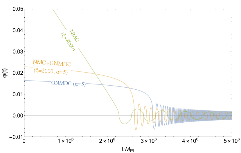
Figure 1: The evolution of the scalar field in three different cases: For GNMDC with $\alpha=5$, for NMC with $\xi\approx 8000$ and for the combination of NMC+GNMDC with $\alpha=5$ and $\xi=2000$, respectively. All three models yield 60 e-folds and $\mathcal{P}_{\mathcal{R}}=2.2\cdot 10^{-9}$. One can observe the lengthening of the period of oscillations, as well as the larger initial value of the field, in the case where NMC becomes more important ($\xi$ grows). Finally, note that when the two theories are combined, $\xi\phi_{*}^{2}$ remains less than $M_{Pl}$.

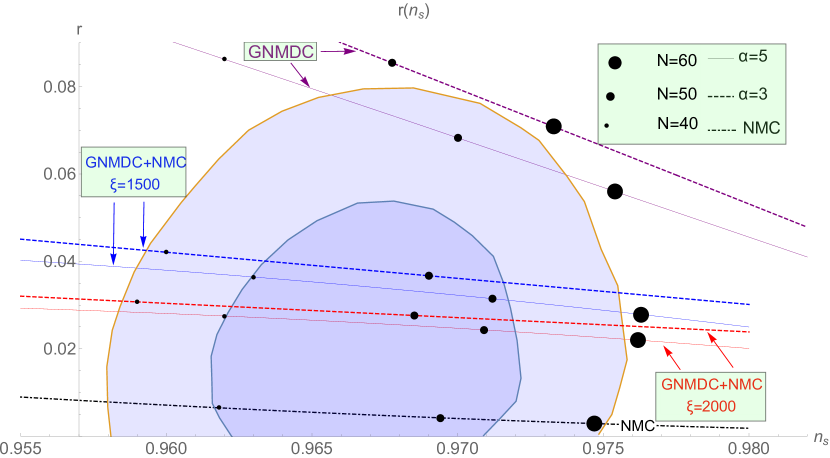
Figure 2: 1$\sigma$ (purple) and 2$\sigma$ (light purple) contours for Planck 2018 results (Planck $+TT+lowP$) [108], on the $r-n_{s}$ plane, alongside the predictions of the scenarios at hand. The NMC scenario corresponds to the dot-dashed line. For the GNMDC (purple lines) we have chosen to show two cases, one with $\alpha=3$ (dashed line) and one with $\alpha=5$ (dotted line). The same convention is used for the combined NMC+GNMDC scenario in terms of $\alpha$, where we also have the colour code of blue lines for $\xi=1500$ and red lines for $\xi=2000$. It is evident that the NMC term lowers the $r$ value as it becomes more significant, as compared to the GNMDC alone. Very low $r$-values are a main feature of NMC of the form $\phi^{2}$. Moreover, one observes that for the same value of $\xi$, as $\alpha$ grows $r$ is also lowered, as reported in [94] too. Finally, the growing dots represent 40, 50 and 60 e-folds respectively.

As a next step we calculate the inflationary observables, and in particular the scalar spectral index and the tensor to scalar ratio, using the exact expressions of Appendix A. In Fig. 2, we present the obtained results for the standalone cases of NMC and of GNMDC, as well as for the combined scenario. Additionally, for transparency, in the same figure we provide the 1$\sigma$ and 2$\sigma$ contours of the Planck 2018 data [108]. As we observe, the simple NMC gives very satisfactory predictions however due to the unitarity violation this model has to be abandoned. The simple GNMDC scenario solves the unitarity issue however it leads to quite large $r$ values and moreover it leads to instabilities related to $c_{s}^{2}$. We observe that, in the combined NMC+GNMDC scenario which alleviates the unitarity issue, one can improve the obtained $r$ values, bringing them back inside the Planck 2018 contours, and moreover the larger the $\alpha$ value is the larger is the improvement. Specifically, one observes that for the same value of $\alpha$ (dashed lines for $\alpha=3$, dotted lines for $\alpha=5$), as $\xi$ grows the tensor-to-scalar ratio lowers. Moreover, for the same value of $\xi$ (blue lines for $\xi=1500$, red lines for $\xi=2000$), as $\alpha$ grows, $r$ also lowers. This result is also expected since this is one of the effects of the sole GNMDC term [94].

In conclusion, monomial GNMDC models with larger $\alpha$ would in fact be more desirable in the context of the combined theory proposed in this work, due to the enhancement of the gravitational friction effect that the $\alpha$ parameter essentially quantifies. However, if one considers a polynomial GNMDC the same effect can actually be obtained, since inflation can be carried by two or more “frictious” terms present in a polynomial GNMDC. We demonstrate such a scenario later.

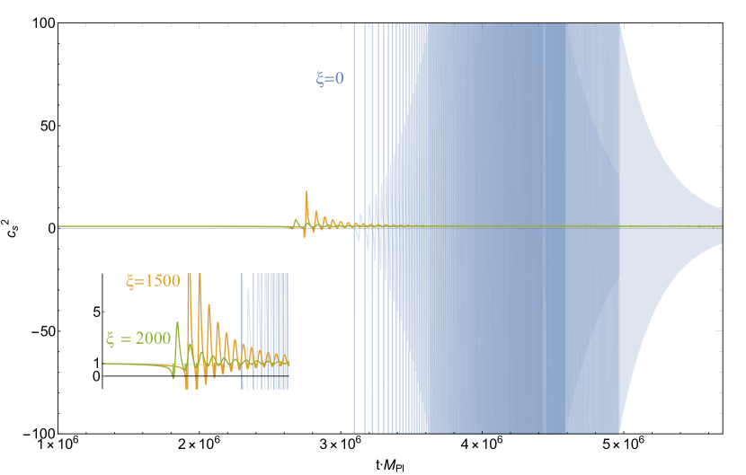
Figure 3: The squared sound speed evolution for the scenario at hand, for $\alpha=5$, with $\xi=0,1500$ and $2000$ respectively. It is clear that as the NMC contribution becomes more significant ($\xi$ increases), the oscillations in its value are damped and $c_{s}^{2}$ is corrected towards 1.

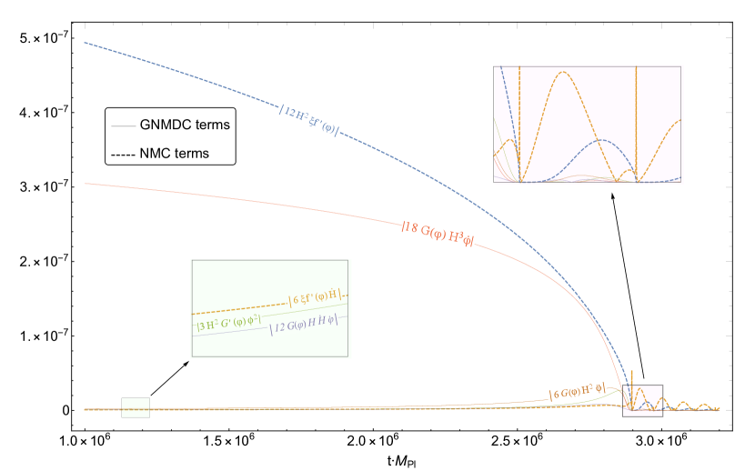
Figure 4: The contribution of the terms related to the GNMDC (continuous lines) and to the NMC (dashed lines) in the Klein-Gordon equation (III.1), for $\alpha=5$ and $\xi=2000$. It is clear than when the oscillations start, the NMC terms dominate over the GNMDC terms and hence the GNMDC effects are negligible, even though during the slow-roll era they are comparable. The standard GR terms are intentionally omitted in order to make the graph simpler.

Let us now examine the evolution of $c_{s}^{2}$ in order to verify that the combined scenario can indeed heal the $c_{s}^{2}$-instabilities of the standalone GNMDC. In Fig. 3 we depict the evolution of $c_{s}^{2}$ for various cases. As one can clearly see, while in the standalone GNMDC (i.e. for $\xi=0$) the $c_{s}^{2}$ wildly oscillates between positive and negative values, when we switch on the NMC contribution we obtain a significant decrease of the oscillatory behavior and a stabilization to positive values. In particular, in the combined scenario we observe that near the end of inflation the GNMDC contribution smooths out, while the NMC term remains co-leading alongside the standard GR (i.e. of the minimally coupled scalar field) terms. However, it is known that the standalone NMC as well as the GR terms have no instability issues. Hence, the $c_{s}^{2}<0$ problem is healed.

In order to provide a more transparent picture of the above relative effect of the GNMDC and the NMC contributions, in Fig. 4 we present the contribution of the terms related to the GNMDC and the NMC in the Klein-Gordon equation (III.1). From this graph it becomes clear that although during the slow-roll era the contributions from NMC and GNMDC are comparable, when the oscillations start the NMC terms dominate completely over the GNMDC terms and since NMC alone leads to $c_{s}^{2}=1$ its complete dominance in the combined model is adequate to bring $c_{s}^{2}$ away from the unstable region (caused by standalone GNMDC). Hence, the GNMDC contribution to the $c_{s}^{2}$ at the end of inflation is overpowered by the NMC contribution and the wild oscillations of the sound speed are damped much earlier in this scenario. Note that this damping of oscillations is more efficient for larger $\alpha$ values, which as we mentioned above lead also to better $r$ values. Hence, overall, larger $\alpha$ values would be more desirable.

This brings up the question of whether this is a realistic scenario. Quantum corrections should, in fact, bring about terms that might be of lower order, so one should check the resulting phenomenology. However, if one chooses a polynomial form for $G(\phi)$, a very similar phenomenology occurs, since, unless the various terms of the polynomial are finely tuned, there will still be only one monomial term that drives the slow roll and hence it will produce very similar results.

Moreover, even in the case that two, or more, terms are actually of the same order of magnitude, the phenomenology is still, qualitatively, the same, since the results of Section III are independent of the exact form of the GNMDC. They are only based on the fact that the GNMDC should become negligible at the end of inflation. Nevertheless, we later provide a numerical example of such a scenario for demonstrative purposes.

In conclusion, in the combined scenario, when inflation starts, the gravitational friction effect due to the GNMDC term is what causes the model to produce a significant amount of e-folds without having to resort to $\xi\phi_{*}^{2}>M_{Pl}$ values as in the standalone NMC case, and this is what alleviates the unitarity issue. At the same time, the NMC term causes the $r$ of the model to be significantly lowered, and thus be in better agreement with observations, as compared to the standalone GNMDC case. Finally, when inflation ends and the oscillations start, the NMC terms remain more significant than that of the GNMDC, which leads to the fast eradication of the oscillations in the $c_{s}^{2}$ value, healing the theory of instabilities. These features and advantages of the combined scenario are amongst the main results of the present work.

Before closing this section, we note another role of the GNMDC parameter $\alpha$ on the results. In the combined scenario even $\alpha$ values can still lead to viable inflation. This is not the case when GNMDC is considered alone [94] due to its inability to satisfy the corresponding requirement (III.1), which essentially disqualifies the area of the phase space corresponding to desirable observables. The fact that in the combined scenario all $\alpha$ values can be used, is a significant advance in the richness of the resulting phenomenology.

This also holds for a polynomial GNMDC form: when an even-valued $\alpha$ term becomes important the polynomial GNMDC numerics become unstable due to the above constraint. This can be ameliorated or even healed, when it is combined with NMC.

As a further numerical demonstration of the effects of the NMC+GNMDC scenario we include a model resulting from a polynomial GNMDC form, namely

$$G(\phi)=\sum_{i}\frac{\alpha_{i}\phi^{\alpha_{i}-1}}{2M_{i}^{\alpha_{i}+1}},$$

where $i$ is a subscript that defines which and how many corresponding terms are taken into account. As a demonstration we pick

$$\frac{\alpha\phi^{\alpha-1}}{2M_{1}^{\alpha+1}}+\frac{(\alpha-1)\phi^{\alpha-2}}{2M_{2}^{\alpha}},$$ (69)

with $\alpha=4$, while the NMC coupling is $\kappa\approx 2000$. The coupling coefficients should be such that these two terms as a whole are of comparable magnitude. If not, then one of the terms would dominate during slow roll, essentially reducing the model to the monomial form presented earlier. We reiterate, that such a scenario is not viable in the sole GNMDC case, since even values of $\alpha$ are problematic.

A polynomial form still falls within the ansatz needed for the results of Section III to hold, namely that the GNMDC becomes negligible near the end of inflation. The results shown therein, then, still hold, since this modification affects only the exact form of the $\epsilon_{G_{i}}$ parameters, and not their overall behavior.

Definitely, picking initial conditions and scales for the combined theory, with a polynomial GNMDC, is a tedious task as compared to the monomial case. Nevertheless, by imposing the ansatz discussed earlier, regarding the magnitude of the various terms of the GNMDC, one can obtain results that are well within observational bounds. The overall picture is very similar to the monomial case, as one can see in Fig. 5, which was expected since the $\epsilon_{G_{i}}$ show a similar behavior.

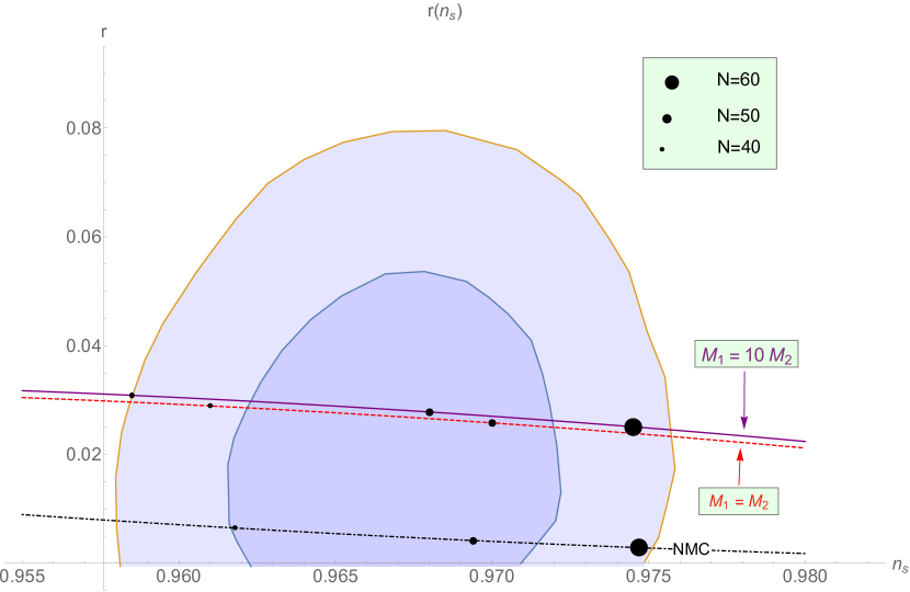
Figure 5: 1$\sigma$ (purple) and 2$\sigma$ (light purple) contours for Planck 2018 results (Planck $+TT+lowP$) [108], on the $r-n_{s}$ plane, alongside the predictions of the polynomial GNMDC+NMC scenario. To demonstrate that the resulting phenomenology is very similar to the monomial case of Fig. 2, we present two cases, one with $M_{1}=M_{2}$ and one with $M_{1}=10M_{2}$. The growing dots represent 40, 50 and 60 e-folds respectively. The corresponding models when NMC is not included are not stable due to the constraint (III.1).

V Conclusions

It is widely accepted that for modern Cosmology to explain the hot big bang and the primordial perturbations observed through the CMBR it has to be complemented by an initial inflationary period. There is a variety of ways to achieve inflation, the most well-studied of which is the inclusion of a scalar field, that through its dynamics affects the evolution of the infant Universe. Given that the only scalar field actually observed in nature up to now is the Higgs field, it would be the prime candidate for such a scenario.

The basic scenarios in which the Higgs field is minimally coupled to gravity have been excluded from Planck observations [108]. The next candidate is to allow the Higgs field to couple nonminimally (NMC) with gravity. NMC Higgs inflation, with a quadratic coupling of the form $f(\phi)=\phi^{2}$, has been shown to yield results in very good agreement with the observations, and particularly low tensor-to-scalar ratio, while the squared sound speed of the scalar perturbations is identically equal to 1 and thus the scenario is free from instabilities. However, this model leads to unitarity violation which in turn is undesirable if one wished to quantize the theory.

The consideration of nonminimal derivative couplings of the scalar field to gravity is shown to solve the unitarity issue, while still leading to satisfactory inflationary observables, due to the presence of a “gravitational friction” that lowers the initial values needed to produce a long slow-roll period and thus a significant amount of e-folds. Nevertheless, these models lead to perturbative instabilities and in particular to $c_{s}^{2}<0$. Although one could construct generalized versions of nonminimal derivative couplings (GNMDC) that could improve the instability issue, considering for instance a coupling function of the form $\frac{\alpha\phi^{\alpha-1}}{M^{\alpha+1}}$, potential problematic behavior still remains.

In this work we constructed the combined scenario of NMC and of GNMDC, which maintain the advantages of the individual models, but remove their individual disadvantages. In the combined scenario, a long enough inflationary phase can be easily achieved, while the initial value of the scalar field and the scale of the NMC term are such that it remains sub-Planckian, a feature not possible in the single field NMC scenario. These attractive features are achieved due to the GNMDC term, that brings about the gravitational friction effect that extends the slow-roll phase, allowing for lower initial values of $\phi_{*}$. Additionally, near the end of inflation, at the bottom of the potential, when a suitable GNMDC term is chosen, it becomes negligible, while the NMC term dominates completely.

To demonstrate this, we have chosen to include two examples, one with a GNMDC of monomial form and one of polynomial form that satisfy the above ansatz (however, other GNMDC forms should also be viable, as long as they become negligible at the end of inflation). In both cases we show that a desirable phenomenology is achieved. At the same time, at the end of inflation canonical gravity is restored, and the scenario is healed from $c_{s}^{2}$-instabilities due to wild oscillations, and with no superluminal scalar perturbations that are related to the simple NMDC case. Finally, another advantage of the present construction is that since the GNMDC contribution becomes negligible after inflation ends, the theory can easily pass the recent LIGO-VIRGO contstraints on the gravitational wave speed [109, 110] (since it is known that the nonminimal derivative coupling terms are amongst the ones that lead to a gravitational wave speed different than one).

In summary, the combined scenario leads to inflationary observables in agreement with observations, it is free from $c_{s}^{2}$-instabilities, and it alleviates the unitarity issue. Hence, it does maintain the advantages of the individual scenarios without sharing their disadvantages. Thus, inflationary scenarios with nonminimal and derivative couplings to gravity combined, may serve as successful candidates for the description of inflationary dynamics, and other mechanisms related to inflation, like Primordial Black Hole formation, and deserve further investigation.

Appendix A Perturbative Analysis of Single Field Inflation

For the perturbative analysis presented here briefly, we mainly follow [25, 91, 103, 104]. The second order action of the curvature perturbation written in the unitary gauge $\mathcal{R}$, is of the form

$$S_{\mathcal{R}}^{(2)}=\int dtd^{3}xa^{3}\left[\mathcal{G}_{S}\dot{\mathcal{R}}^{2}-\frac{\mathcal{F}_{S}}{a^{2}}(\partial\mathcal{R})^{2}\right]~{},$$ (70)

where $a$ is the scale factor, and with the definitions

$$\mathcal{G}_{S} \equiv\frac{\Sigma}{\Theta^{2}}\mathcal{G}_{T}^{2}+3\mathcal{G}_{T}~{}, \mathcal{F}_{S} \equiv\frac{1}{a}\frac{d}{dt}\left(\frac{a}{\Theta}\mathcal{G}_{T}^{2}\right)-\mathcal{F}_{T}~{}.$$ (71)

$\Sigma,\Theta,\mathcal{G}_{T}$ and $\mathcal{F}_{T}$ are functions that depend on the Galileon functions and the derivatives of the field (see [104]). Specifically

$$\mathcal{G}_{T}\equiv 2\left[G_{4}-2XG_{4X}-X\left(H\dot{\phi}G_{5X}-G_{5\phi}\right)\right]~{},$$ (72)

$$\!\!\!\!\!\!\!\!\!\!\!\!\!\!\!\!\!\!\!\!\!\!\!\!\!\!\!\!\!\!\!\!\!\!\!\!\!\!\!\!\!\!\!\!\!\!\!\mathcal{F}_{T}\equiv 2\left[G_{4}-X\left(\ddot{\phi}G_{5X}+G_{5\phi}\right)\right]~{},$$ (73)

$$\Theta \equiv-\dot{\phi}XG_{3X}+2H\left(G_{4}-4XG_{4X}-4X^{2}G_{4XX}\right)$$

$$+\dot{\phi}\left(G_{4\phi}+2XG_{4\phi X}\right)-H^{2}\dot{\phi}\left(5XG_{5X}+2X^{2}G_{5XX}\right)$$

$$+2HX\left(3G_{5\phi}+2XG_{5\phi X}\right)~{},$$ (74)

$$\Sigma\equiv X\left(G_{2X}+2XG_{2XX}\right)+6H\dot{\phi}X\left(2G_{3X}+XG_{3XX}\right)$$

$$\!-2X\left(G_{3\phi}+XG_{3\phi X}\right)-6H^{2}G_{4}$$

$$\!+6\left[H^{2}\left(7XG_{4X}+16X^{2}G_{4XX}+4X^{3}G_{4XXX}\right)\right.$$

$$\!\left.-H\dot{\phi}\left(G_{4\phi}+5XG_{4\phi X}+2X^{2}G_{4\phi XX}\right)\right]$$

$$\!+H^{3}\dot{\phi}X\left(30G_{5X}+26XG_{5XX}+4X^{2}G_{5XXX}\right)$$

$$\!-6H^{2}X\left(6G_{5\phi}+9XG_{5\phi X}+2X^{2}G_{5\phi XX}\right)~{}.$$ (75)

Then, with specified Galileon functions, one can calculate the squared sound speed of the scalar and tensorial perturbations via the formulas

$$c_{s}^{2} \equiv\frac{\mathcal{F}_{S}}{\mathcal{G}_{S}}~{}, c_{T}^{2} \equiv\frac{\mathcal{F}_{T}}{\mathcal{G}_{T}}~{}.$$ (76)

These quantities have to be positive in order to avoid gradient instabilities, i.e. exponential growth of perturbation modes. On the same footing, to ensure that the kinetic terms are positive and no ghost instabilities appear, the constraints

$$\mathcal{G}_{S}>0~{},~{}~{}~{}~{} \mathcal{G}_{T}>0~{},$$ (77)

must hold, too. For instance, in the NMC scenario, using equations (4),(II.1) and (6), it is straightforward to prove that $c_{s}^{2}=1$, hence no corresponding instabilities occur.

Furthermore, one can show that in order to calculate the Power Spectrum of the scalar and tensorial perturbations, one simply needs to calculate [111]

$$\mathcal{P}_{\mathcal{R}}=\frac{\mathcal{G}_{S}^{1/2}}{2\mathcal{F}_{S}^{3/2}}\frac{H^{2}}{4\pi^{2}}~{},\ \mathcal{P}_{\mathcal{T}}=\frac{8\mathcal{G}_{T}^{1/2}}{\mathcal{F}_{T}^{3/2}}\frac{H^{2}}{4\pi^{2}}~{},$$ (78)

which are evaluated at the horizon crossing. Their quotient is the tensor-to-scalar ratio $r$, namely

$$r\equiv\frac{\mathcal{P}_{\mathcal{T}}}{\mathcal{P}_{\mathcal{R}}}~{}.$$ (79)

Furthermore, we introduce the scalar spectral index, $n_{s}$, expressing the change of the logarithm of the scalar power spectrum per logarithmic interval $k$, via the relation

$$1-n_{s}\equiv-\frac{d\ln\mathcal{P}_{\mathcal{R}}}{d\ln k}\Big{|}_{k=aH}~{},$$ (80)

and likewise, the tensorial spectral index

$$n_{t}\equiv-\frac{d\ln\mathcal{P}_{\mathcal{T}}}{d\ln k}\Big{|}_{k=aH}~{}.$$ (81)

The tensor-to-scalar ratio and the tensor tilt are related via what is called the consistency condition and in standard single-field inflation it takes the form $r\approx-8n_{t}$, nevertheless in modified scenarios its form can be non-standard. In summary, the observables of an inflationary model are $r,n_{s}$ and $\mathcal{P}_{\mathcal{R}}$.

References

- [1] K. A. Olive, Inflation, Phys. Rept. 190, 307 (1990).
- [2] D. H. Lyth and A. Riotto, Particle physics models of inflation and the cosmological density perturbation, Phys. Rept. 314, 1-146 (1999) [arXiv:hep-ph/9807278].
- [3] J. Martin, C. Ringeval and V. Vennin, Encyclopædia Inflationaris, Phys. Dark Univ. 5-6, 75-235 (2014) [arXiv:1303.3787 [astro-ph.CO]].
- [4] M. Yu. Khlopov, Primordial Black Holes, Res. Astron. Astrophys. 10, 495-528 (2010) [arXiv:0801.0116 [astro-ph]].
- [5] S. Chongchitnan and G. Efstathiou, Accuracy of slow-roll formulae for inflationary perturbations: implications for primordial black hole formation, JCAP 0701 (2007) 011 [astro-ph/0611818].
- [6] J. Garcia-Bellido and E. Ruiz Morales, Primordial black holes from single field models of inflation, Phys. Dark Univ. 18 (2017) 47 [arXiv:1702.03901 [astro-ph.CO]].
- [7] Y. F. Cai, X. Tong, D. G. Wang and S. F. Yan, Primordial Black Holes from Sound Speed Resonance during Inflation, Phys. Rev. Lett. 121 (2018) no.8, 081306 [arXiv 1805.03639 [astro-ph.CO]].
- [8] G. Ballesteros, J. Beltran Jimenez and M. Pieroni, Black hole formation from a general quadratic action for inflationary primordial fluctuations, JCAP 1906 (2019) 016 [arXiv:1811.03065 [astro-ph.CO]].
- [9] C. Chen and Y. F. Cai, Primordial black holes from sound speed resonance in the inflaton-curvaton mixed scenario, JCAP 10, 068 (2019) [arXiv:1908.03942 [astro-ph.CO]].
- [10] C. Germani and I. Musco, Abundance of Primordial Black Holes Depends on the Shape of the Inflationary Power Spectrum, Phys. Rev. Lett. 122 (2019) no.14, 141302 [arXiv:1805.04087 [astro-ph.CO]].
- [11] C. Fu, P. Wu and H. Yu, Primordial Black Holes from Inflation with Nonminimal Derivative Coupling, Phys. Rev. D 100, no. 6, 063532 (2019) [arXiv:1907.05042 [astro-ph.CO]].
- [12] Y. Lu, Y. Gong, Z. Yi and F. Zhang, Constraints on primordial curvature perturbations from primordial black hole dark matter and secondary gravitational waves, JCAP 12, 031 (2019) [arXiv:1907.11896 [gr-qc]].
- [13] I. Dalianis, Constraints on the curvature power spectrum from primordial black hole evaporation, JCAP 2019 (2019) no.08, 032 [arXiv:1812.09807 [astro-ph.CO]].
- [14] Z. Yi, Q. Gao, Y. Gong and Z. h. Zhu, Primordial black holes and secondary gravitational waves from inflationary model with a non-canonical kinetic term, [arXiv:2011.10606 [astro-ph.CO]].
- [15] Z. Yi, Y. Gong, B. Wang and Z. h. Zhu, Primordial Black Holes and Secondary Gravitational Waves from Higgs field, [arXiv:2007.09957 [gr-qc]].
- [16] S. Pi, Y. Zhang, Q. G. Huang and M. Sasaki, Scalaron from -gravity as a Heavy Field, JCAP 05 (2018) 042, [arXiv:1712.09896 [astro-ph.CO]]
- [17] D. J. Gross and J. H. Sloan, The Quartic Effective Action for the Heterotic String, Nucl. Phys. B 291, 41 (1987).
- [18] Y. Fujii and K. Maeda, The scalar-tensor theory of gravitation, Cambridge University Press, Cambridge (2003).
- [19] G. W. Horndeski, Second-order scalar-tensor field equations in a four-dimensional space, Int. J. Theor. Phys. 10 (1974) 363.
- [20] M. Ostrogradsky, Memoires sur les equations differentielles, relatives au probleme des isoperimetres, Mem. Acad. St. Petersbourg 6, no. 4, 385 (1850).
- [21] A. Nicolis, R. Rattazzi, E. Trincherini, The Galileon as a local modification of gravity, Phys. Rev. D79 (2009) 064036. [arXiv:0811.2197 [hep-th]].
- [22] C. Deffayet, G. Esposito-Farese, A. Vikman, Covariant Galileon, Phys. Rev. D79 (2009) 084003. [arXiv:0901.1314 [hep-th]].
- [23] C. Deffayet, S. Deser and G. Esposito-Farese, Generalized Galileons: All scalar models whose curved background extensions maintain second-order field equations and stress-tensors, Phys. Rev. D 80, 064015 (2009). [arXiv:0906.1967].
- [24] C. Deffayet, X. Gao, D. A. Steer and G. Zahariade, From k-essence to generalised Galileons, Phys. Rev. D 84, 064039 (2011). [arXiv:1103.3260 [hep-th]].
- [25] T. Kobayashi, M. Yamaguchi and J. Yokoyama, Generalized G-inflation: Inflation with the most general second-order field equations, Prog. Theor. Phys. 126 (2011) 511 [arXiv:1105.5723 [hep-th]].
- [26] T. Harko, F. S. N. Lobo, E. N. Saridakis and M. Tsoukalas, Cosmological models in modified gravity theories with extended nonminimal derivative couplings, Phys. Rev. D 95, no.4, 044019 (2017) [arXiv:1609.01503 [gr-qc]].
- [27] K. Kamada, T. Kobayashi, M. Yamaguchi and J. Yokoyama, Higgs G-inflation, Phys. Rev. D 83 (2011) 083515 [arXiv:1012.4238 [astro-ph.CO]].
- [28] E. N. Saridakis, R. Lazkoz, V. Salzano, P. Vargas Moniz, S. Capozziello, et al. Modified Gravity and Cosmology: An Update by the CANTATA Network, [arXiv:2105.12582 [gr-qc]].
- [29] D. S. Salopek, J. R. Bond and J. M. Bardeen, Designing Density Fluctuation Spectra in Inflation, Phys. Rev. D 40, 1753 (1989).
- [30] R. Fakir and W. G. Unruh, Improvement on cosmological chaotic inflation through nonminimal coupling, Phys. Rev. D 41, 1783 (1990).
- [31] D. I. Kaiser, Primordial spectral indices from generalized Einstein theories, Phys. Rev. D 52 (1995) 4295 [arXiv:astro-ph/9408044].
- [32] E. Komatsu and T. Futamase, Complete constraints on a nonminimally coupled chaotic inflationary scenario from the cosmic microwave background, Phys. Rev. D 59 (1999) 064029, [arXiv:astro-ph/9901127].
- [33] K. Nozari and S. D. Sadatian, Non-Minimal Inflation after WMAP3, Mod. Phys. Lett. A 23 (2008) 2933 [arXiv:0710.0058 [astro-ph]].
- [34] J. Ren, Z. Xianyu and H. He, Higgs Gravitational Interaction, Weak Boson Scattering, and Higgs Inflation in Jordan and Einstein Frames, JCAP 06, 032 (2014) [arXiv:1404.4627 [gr-qc]]
- [35] S. C. Park and S. Yamaguchi, Inflation by non-minimal coupling, JCAP 08, 009 (2008) [arXiv:0801.1722 [hep-ph]].
- [36] A. Ashoorioon and K. Rezazadeh, Non-Minimal M-flation, JHEP 07, 244 (2020)
- [37] F. L. Bezrukov and M. Shaposhnikov, The Standard Model Higgs boson as the inflaton, Phys. Lett. B 659, 703 (2008), [arXiv:0710.3755 [hep-th]].
- [38] A. O. Barvinsky, A. Y. Kamenshchik and A. A. Starobinsky, Inflation scenario via the Standard Model Higgs boson and LHC, JCAP 0811 (2008) 021, [arXiv:0809.2104 [hep-ph]].
- [39] F. Bezrukov, D. Gorbunov and M. Shaposhnikov, On initial conditions for the Hot Big Bang, JCAP 06, 029 (2009) [arXiv:0812.3622 [hep-ph]].
- [40] J. Garcia-Bellido, D. G. Figueroa and J. Rubio, Preheating in the Standard Model with the Higgs-Inflaton coupled to gravity, Phys. Rev. D 79, 063531 (2009) [arXiv:0812.4624 [hep-ph]].
- [41] A. De Simone, M. P. Hertzberg and F. Wilczek, Running Inflation in the Standard Model, Phys. Lett. B 678, 1-8 (2009) [arXiv:0812.4946 [hep-ph]].
- [42] F. L. Bezrukov, A. Magnin and M. Shaposhnikov, Standard Model Higgs boson mass from inflation, Phys. Lett. B 675, 88-92 (2009) [arXiv:0812.4950 [hep-ph]].
- [43] C. P. Burgess, H. M. Lee and M. Trott, Power-counting and the Validity of the Classical Approximation During Inflation, JHEP 09, 103 (2009) [arXiv:0902.4465 [hep-ph]].
- [44] J. L. F. Barbon and J. R. Espinosa, On the Naturalness of Higgs Inflation, Phys. Rev. D 79, 081302 (2009) [arXiv:0903.0355 [hep-ph]].
- [45] F. Bezrukov and M. Shaposhnikov, Standard Model Higgs boson mass from inflation: two loop analysis, JHEP 07, 089 (2009) [arXiv:0904.1537 [hep-ph]].
- [46] A. O. Barvinsky, A. Y. Kamenshchik, C. Kiefer, A. A. Starobinsky and C. Steinwachs, Asymptotic freedom in inflationary cosmology with a non-minimally coupled Higgs field, JCAP 12, 003 (2009) [arXiv:0904.1698 [hep-ph]].
- [47] T. E. Clark, B. Liu, S. T. Love and T. ter Veldhuis, The Standard Model Higgs Boson-Inflaton and Dark Matter, Phys. Rev. D 80, 075019 (2009) [arXiv:0906.5595 [hep-ph]].
- [48] A. O. Barvinsky, A. Y. Kamenshchik, C. Kiefer, A. A. Starobinsky and C. F. Steinwachs, Higgs boson, renormalization group, and naturalness in cosmology, Eur. Phys. J. C 72, 2219 (2012) [arXiv:0910.1041 [hep-ph]].
- [49] M. B. Einhorn and D. R. T. Jones, Inflation with Non-minimal Gravitational Couplings in Supergravity, JHEP 03, 026 (2010) [arXiv:0912.2718 [hep-ph]].
- [50] R. N. Lerner and J. McDonald, Higgs Inflation and Naturalness, JCAP 04, 015 (2010) [arXiv:0912.5463 [hep-ph]].
- [51] C. P. Burgess, H. M. Lee and M. Trott, Comment on Higgs Inflation and Naturalness, JHEP 07, 007 (2010) [arXiv:1002.2730 [hep-ph]].
- [52] A. Mazumdar and J. Rocher, Particle physics models of inflation and curvaton scenarios, Phys. Rept. 497, 85-215 (2011) [arXiv:1001.0993 [hep-ph]].
- [53] C. Q. Geng, C. C. Lee, M. Sami, E. N. Saridakis and A. A. Starobinsky, Observational constraints on successful model of quintessential Inflation, JCAP 06, 011 (2017) [arXiv:1705.01329 [gr-qc]].
- [54] J. Fumagalli and M. Postma, UV (in)sensitivity of Higgs inflation, JHEP 05, 049 2016, [arXiv:1602.07234[hep-ph]]
- [55] M. P. Hertzberg, On Inflation with Non-minimal Coupling, JHEP 11, 023 (2010) [arXiv:1002.2995 [hep-ph]].
- [56] G. F. Giudice and H. M. Lee, Unitarizing Higgs Inflation, Phys. Lett. B 694, 294-300 (2011) [arXiv:1010.1417 [hep-ph]].
- [57] T. Tenkanen, Resurrecting Quadratic Inflation with a non-minimal coupling to gravity, JCAP 12, 001 (2017) [arXiv:1710.02758 [astro-ph.CO]].
- [58] J. McDonald, Does Palatini Higgs Inflation Conserve Unitarity, arXiv:2007.04111
- [59] T. Tenkanen and E. Tomberg, Initial conditions for plateau inflation: a case study, JCAP 04, 050 (2020) [arXiv:2002.02420 [astro-ph.CO]].
- [60] R. N. Lerner and J. McDonald, A Unitarity-Conserving Higgs Inflation Model, Phys. Rev. D 82, 103525 (2010) [arXiv:1005.2978 [hep-ph]].
- [61] S. Lola, A. Lymperis and E. N. Saridakis, Inflation with non-canonical scalar fields revisited, [arXiv:2005.14069 [gr-qc]].
- [62] T. Kolyvaris, G. Koutsoumbas, E. Papantonopoulos and G. Siopsis, Scalar Hair from a Derivative Coupling of a Scalar Field to the Einstein Tensor, Class. Quant. Grav. 29, 205011 (2012), [arXiv:1111.0263 [gr-qc]].
- [63] M. Rinaldi, Black holes with non-minimal derivative coupling, Phys. Rev. D 86, 084048 (2012) [arXiv:1208.0103 [gr-qc]].
- [64] T. Kolyvaris, G. Koutsoumbas, E. Papantonopoulos and G. Siopsis, Phase Transition to a Hairy Black Hole in Asymptotically Flat Spacetime, JHEP 1311, 133 (2013), [arXiv:1308.5280 [hep-th]].
- [65] E. Babichev and C. Charmousis, Dressing a black hole with a time-dependent Galileon, JHEP 08, 106 (2014) [arXiv:1312.3204 [gr-qc]].
- [66] A. Cisterna and C. Erices, Asymptotically locally AdS and flat black holes in the presence of an electric field in the Horndeski scenario, Phys. Rev. D 89, 084038 (2014) [arXiv:1401.4479 [gr-qc]].
- [67] C. Charmousis, T. Kolyvaris, E. Papantonopoulos and M. Tsoukalas, Black Holes in Bi-scalar Extensions of Horndeski Theories, JHEP 07, 085 (2014) [arXiv:1404.1024 [gr-qc]].
- [68] G. Koutsoumbas, K. Ntrekis, E. Papantonopoulos and M. Tsoukalas, Gravitational Collapse of a Homogeneous Scalar Field Coupled Kinematically to Einstein Tensor, Phys. Rev. D 95, no.4, 044009 (2017) [arXiv:1512.05934 [gr-qc]].
- [69] A. Anabalon, A. Cisterna and J. Oliva, Asymptotically locally AdS and flat black holes in Horndeski Theory, Phys. Rev. D 89, 084050 (2014), [arXiv:1312.3597 [gr-qc]]
- [70] A. Cisterna, T. Delsate and M. Rinaldi, Neutron Stars in general second order scalar-tensor theory: the case of non-minimal derivative coupling, Phys. Rev. D 92, 044050 (2015), [arXiv:1504.05189 [gr-qc]]
- [71] A. Cisterna, T. Delsate, L. Ducobu and M. Rinaldi, Slowly rotating neutron stars in the nonminimal derivative coupling sector of Horndeski gravity, Phys. Rev. D 93, 084046 (2016), [arXiv:1602.06939 [gr-qc]]
- [72] E. N. Saridakis and S. V. Sushkov, Quintessence and phantom cosmology with non-minimal derivative coupling, Phys. Rev. D 81, 083510 (2010) [arXiv:1002.3478 [gr-qc]].
- [73] J. B. Dent, S. Dutta, E. N. Saridakis and J. Q. Xia, Cosmology with non-minimal derivative couplings:perturbation analysis and observational constraints, JCAP 11, 058 (2013) [arXiv:1309.4746 [astro-ph.CO]].
- [74] L. Amendola, Cosmology with nonminimal derivative couplings, Phys. Lett. B 301, 175 (1993) [arXiv:gr-qc/9302010].
- [75] H. Sheikhahmadi, E. N. Saridakis, A. Aghamohammadi and K. Saaidi, Hamilton-Jacobi formalism for inflation with non-minimal derivative coupling, JCAP 10, 021 (2016) [arXiv:1603.03883 [gr-qc]].
- [76] E. Papantonopoulos, Effects of the kinetic coupling of matter to curvature, Int. J. Mod. Phys. D 28, no. 05, 1942007 (2019).
- [77] C. Germani, N. Kudryashova and Y. Watanabe, On post-inflation validity of perturbation theory in Horndeski scalar-tensor models, JCAP 1608 (2016) 015 [arXiv:1512.06344 [astro-ph.CO]].
- [78] S. V. Sushkov, Exact cosmological solutions with nonminimal derivative coupling, Phys. Rev. D 80, 103505 (2009) [arXiv:0910.0980 [gr-qc]].
- [79] C. Germani and A. Kehagias, New Model of Inflation with Non-minimal Derivative Coupling of Standard Model Higgs Boson to Gravity, Phys. Rev. Lett. 105 (2010) 011302, [arXiv:1003.2635 [hep-ph]].
- [80] F. Farakos, C. Germani, A. Kehagias and E. N. Saridakis, A New Class of Four-Dimensional N=1 Supergravity with Non-minimal Derivative Couplings, JHEP 1205 (2012) 050 [arXiv:1202.3780 [hep-th]].
- [81] F. Farakos, C. Germani and A. Kehagias, On ghost-free supersymmetric galileons, JHEP 1311 (2013) 045 [arXiv:1306.2961 [hep-th]].
- [82] I. Dalianis and F. Farakos, Higher Derivative D-term Inflation in New-minimal Supergravity, Phys. Lett. B 736 (2014) 299 [arXiv:1403.3053 [hep-th]].
- [83] I. Dalianis, G. Koutsoumbas, K. Ntrekis and E. Papantonopoulos, Reheating predictions in Gravity Theories with Derivative Coupling, JCAP 1702, no. 02, 027 (2017) [arXiv:1608.04543 [gr-qc]].
- [84] H. M. Sadjadi and P. Goodarzi, Reheating in nonminimal derivative coupling model, JCAP 1302 (2013) 038, [arXiv:1203.1580 [gr-qc]].
- [85] A. Ghalee, A new phase of scalar field with a kinetic term non-minimally coupled to gravity, Phys. Lett. B 724 (2013) 198, [arXiv:1303.0532 [astro-ph.CO]].
- [86] N. Yang, Q. Fei, Q. Gao and Y. Gong, Inflationary models with non-minimally derivative coupling, Class. Quant. Grav. 33, no.20, 205001 (2016) [arXiv:1504.05839 [gr-qc]].
- [87] B. Gumjudpai and P. Rangdee, Non-minimal derivative coupling gravity in cosmology, Gen. Rel. Grav. 47, no. 11, 140 (2015), [arXiv:1511.00491 [gr-qc]].
- [88] Z. Yi and Y. Gong, Nonminimal coupling and inflationary attractors, Phys. Rev. D 94, no.10, 103527 (2016) [arXiv:1608.05922 [gr-qc]].
- [89] I. D. Gialamas, A. Karam, A. Lykkas and T. D. Pappas, Palatini-Higgs inflation with nonminimal derivative coupling, Phys. Rev. D 102, no.6, 063522 (2020) [arXiv:2008.06371 [gr-qc]].
- [90] Y. S. Myung and T. Moon, Inflaton decay and reheating in nonminimal derivative coupling, JCAP 1607, 014 (2016) [arXiv:1601.03148 [gr-qc]].
- [91] Y. Ema, R. Jinno, K. Mukaida and K. Nakayama, Particle Production after Inflation with Non-minimal Derivative Coupling to Gravity, JCAP 1510, no. 10, 020 (2015), [arXiv:1504.07119 [gr-qc]].
- [92] Y. Ema, R. Jinno, K. Mukaida and K. Nakayama, Gravitational particle production in oscillating backgrounds and its cosmological implications, Phys. Rev. D 94 (2016) no.6, 063517 [arXiv:1604.08898 [hep-ph]].
- [93] G. Koutsoumbas, K. Ntrekis and E. Papantonopoulos, Gravitational Particle Production in Gravity Theories with Non-minimal Derivative Couplings, JCAP 1308, 027 (2013), [arXiv:1305.5741 [gr-qc]].
- [94] I. Dalianis, S. Karydas and E. Papantonopoulos, Generalized Non-Minimal Derivative Coupling: Application to Inflation and Primordial Black Hole Production, JCAP 06, 040 (2020) [arXiv:1910.00622 [astro-ph.CO]].
- [95] B. P. Abbott et al. [LIGO Scientific and Virgo Collaborations], GW151226: Observation of Gravitational Waves from a 22-Solar-Mass Binary Black Hole Coalescence, Phys. Rev. Lett. 116, no. 24, 241103 (2016) [arXiv:1606.04855 [gr-qc]].
- [96] B. P. Abbott et al. [LIGO Scientific and Virgo Collaborations], Observation of Gravitational Waves from a Binary Black Hole Merger, Phys. Rev. Lett. 116 (2016) no.6, 061102 [arXiv:1602.03837 [gr-qc]].
- [97] T. Baker, E. Bellini, P. G. Ferreira, M. Lagos, J. Noller and I. Sawicki, Strong constraints on cosmological gravity from GW170817 and GRB 170817A, Phys. Rev. Lett. 119, no. 25, 251301 (2017) [arXiv:1710.06394 [astro-ph.CO]].
- [98] P. A. González, M. Olivares, E. Papantonopoulos and Y. Vásquez, Constraints on scalar–tensor theory of gravity by solar system tests, Eur. Phys. J. C 80, no.10, 981 (2020) [arXiv:2002.03394 [gr-qc]].
- [99] J. M. Ezquiaga and M. Zumalacarregui, Dark Energy After GW170817: Dead Ends and the Road Ahead, Phys. Rev. Lett. 119, no. 25, 251304 (2017) [arXiv:1710.05901 [astro-ph.CO]].
- [100] Y. Gong, E. Papantonopoulos and Z. Yi, Constraints on scalar-tensor theory of gravity by the recent observational results on gravitational waves, Eur. Phys. J. C 78, no. 9, 738 (2018) [arXiv:1711.04102 [gr-qc]].
- [101] C. Germani and Y. Watanabe, UV-protected (Natural) Inflation: Primordial Fluctuations and non-Gaussian Features, JCAP 1107, 031 (2011) Addendum: [JCAP 1107, A01 (2011)] [arXiv:1106.0502 [astro-ph.CO]]. 10.1088/1475-7516/2011/07/A01;
- [102] E. N. Saridakis, Do we need soft cosmology?, [arXiv:2105.08646 [astro-ph.CO]].
- [103] S. Tsujikawa, Observational tests of inflation with a field derivative coupling to gravity, Phys. Rev. D 85 (2012) 083518 [arXiv:1201.5926 [astro-ph.CO]].
- [104] T. Kobayashi, Horndeski theory and beyond: a review, Rept.Prog.Phys. 82 (2019) no.8, 086901 [arXiv:1901.07183 [gr-qc]].
- [105] J. Fumagalli, S. Mooij and M. Postma Unitarity and Predictiveness in new Higgs inflation, JHEP 03 2018, 038, [arXiv:1711.08761[hep-ph]]
- [106] J. Fumagalli, M. Postma and M. v. d. Bout Matching and running sensitivity in non-renormalizable inflationary models, JHEP 09 2020, 114, [arXiv:2005.05905[hep-ph]]
- [107] M. Atkins and X. Calmet, Remarks on Higgs Inflation, Phys. Lett. B 697, 37-40 (2011) [arXiv:1011.4179 [hep-ph]].
- [108] Y. Akrami et al. [Planck], Planck 2018 results. X. Constraints on inflation, Astron. Astrophys. 641, A10 (2020) [arXiv:1807.06211 [astro-ph.CO]].
- [109] B. P. Abbott et al. [LIGO Scientific and Virgo Collaborations], GW170817: Observation of Gravitational Waves from a Binary Neutron Star Inspiral, Phys. Rev. Lett. 119, no. 16, 161101 (2017) [arXiv:1710.05832 [gr-qc]].
- [110] A. Goldstein et al., An Ordinary Short Gamma-Ray Burst with Extraordinary Implications: Fermi-GBM Detection of GRB 170817A, Astrophys. J. 848, no. 2, L14 (2017) [arXiv:1710.05446 [astro-ph.HE]].
- [111] V. F. Mukhanov, H. A. Feldman and R. H. Brandenberger, Theory of cosmological perturbations. Part 1. Classical perturbations. Part 2. Quantum theory of perturbations. Part 3. Extensions, Phys. Rept. 215 (1992) 203.