Complex Momentum for Optimization in Games

Abstract

We generalize gradient descent with momentum for optimization in differentiable games to have complex-valued momentum. We give theoretical motivation for our method by proving convergence on bilinear zero-sum games for simultaneous and alternating updates. Our method gives real-valued parameter updates, making it a drop-in replacement for standard optimizers. We empirically demonstrate that complex-valued momentum can improve convergence in realistic adversarial games—like generative adversarial networks—by showing we can find better solutions with an almost identical computational cost. We also show a practical generalization to a complex-valued Adam variant, which we use to train BigGAN to better inception scores on CIFAR-10.

1 Introduction

Gradient-based optimization has been critical for the success of machine learning, updating a single set of parameters to minimize a single loss. A growing number of applications require learning in games, which generalize single-objective optimization. Common examples are GANs [1], actor-critic models [2], curriculum learning [3, 4, 5], hyperparameter optimization [6, 7, 8, 9], adversarial examples [10, 11], learning models [12, 13, 14], domain adversarial adaptation [15], neural architecture search [16, 17], and meta-learning [18, 19].

Games consist of multiple players, each with parameters and objectives. We often want solutions where no player gains from changing their strategy unilaterally, e.g., Nash equilibria [20] or Stackelberg equilibria [21]. Classical gradient-based learning often fails to find these equilibria due to rotational dynamics [22]. Numerous saddle point finding algorithms for zero-sum games have been proposed [23, 24]. Gidel et al. [25] generalizes GD with momentum to games, showing we can use a negative momentum to converge if the eigenvalues of the Jacobian of the gradient vector field have a large imaginary part. We use the terminology in Gidel et al. [25] and say (purely) cooperative or adversarial games for games with (purely) real or imaginary eigenvalues. Setups like GANs are not purely adversarial, but rather have both purely cooperative and adversarial eigenspaces – i.e., eigenspaces with purely real or imaginary eigenvalues. In cooperative eigenspaces, the players do not interfere with each other.

We want solutions that converge with simultaneous and alternating updates in purely adversarial games – a setup where existing momentum methods fail. Also, we want solutions that are robust to different mixtures of adversarial and cooperative eigenspaces, because this depends on the games eigendecomposition which can be intractable. To solve this we unify and generalize existing momentum methods [26, 25] to recurrently linked momentum – a setup with multiple recurrently linked momentum buffers with potentially negative coefficients shown in Figure 2(c).

We show that selecting two of these recurrently linked buffers with appropriate momentum coefficients can be interpreted as the real and imaginary parts of a single complex buffer and complex momentum coefficient – see Figure 2(d). This setup (a) allows us to converge in adversarial games with simultaneous updates, (b) only introduces one new optimizer parameter – the phase or $\arg$ of our momentum, (c) allows us to gain intuitions via complex analysis, (d) is trivial to implement in libraries supporting complex arithmetic, and (e) robustly converges for different eigenspace mixtures.

Intuitively, our complex buffer stores historical gradient information, oscillating between adding or subtracting at a frequency dictated by the momentum coefficient. Classical momentum only adds gradients, and negative momentum changes between adding or subtracting each iteration, while we oscillate at an arbitrary (fixed) frequency – see Figure 3.1. This reduces rotational dynamics during training by canceling out opposing updates.

Contributions

• We provide generalizations and variants of classical [27, 28, 29], negative [25, 30], and aggregated [26] momentum for learning in differentiable games.

• We show our methods converges on adversarial games – including bilinear zero-sum games and the Dirac-GAN – with simultaneous and alternating updates.

• We illustrate a robustness during optimization, converging faster and over a larger range of mixtures of cooperative and adversarial games than existing first-order methods.

• We give a practical extension of our method to a complex-valued Adam [31] variant, which we use to train a BigGAN [32] on CIFAR-10, improving [32]’s inception scores.

Actual JAX implementation: changes in green

⬇

mass = .8 + .3j

def momentum(step_size, mass):

...

def update(i, g, state):

x, velocity = state

velocity = mass * velocity + g

x=x-jnp.real(step_size(i)*velocity)

return x, velocity

...

Figure 1: How to modify JAX’s SGD with momentum here to use complex momentum. The only changes are in green. jnp.real gets the real part of step_size times the momentum buffer (called velocity here). We use a complex mass for our method in this case $\beta=|\beta|\exp(i\arg(\beta))=$0.9$\exp(i\nicefrac{{\pi}}{{$8$}})\approx.8+.3i$.

2 Background

Appendix Table 2 summarizes our notation. Consider the optimization problem:

$$\boldsymbol{\theta}^{*}\vcentcolon=\textnormal{arg\,min}_{\boldsymbol{\theta}}\mathcal{L}(\boldsymbol{\theta})$$ (1)

We can find local minima of loss $\mathcal{L}$ using (stochastic) gradient descent with step size $\alpha$. We denote the loss gradient at parameters $\boldsymbol{\theta}^{j}$ by $\boldsymbol{g}^{j}\!\!\vcentcolon=\!\!\boldsymbol{g}(\boldsymbol{\theta}^{j})\!\!\vcentcolon=\!\!\smash{\left.\nabla_{\boldsymbol{\theta}}\mathcal{L}(\boldsymbol{\theta})\right|_{\boldsymbol{\theta}^{j}}}$.

$$\smash{\boldsymbol{\theta}^{j\!+\!1}=\boldsymbol{\theta}^{j}-\alpha\boldsymbol{g}^{j}}$$ (SGD)

Momentum can generalize SGD. For example, Polyak’s Heavy Ball [27]:

$$\smash{\boldsymbol{\theta}^{j\!+\!1}=\boldsymbol{\theta}^{j}-\alpha\boldsymbol{g}^{j}+\beta(\boldsymbol{\theta}^{j}-\boldsymbol{\theta}^{j-1})}$$ (2)

Which can be equivalently written with momentum buffer $\smash{\boldsymbol{\mu}^{j}=\nicefrac{{(\boldsymbol{\theta}^{j}-\boldsymbol{\theta}^{j-1})}}{{\alpha}}}$.

$$\smash{\boldsymbol{\mu}^{j\!+\!1}=\beta\boldsymbol{\mu}^{j}-\boldsymbol{g}^{j},\quad\quad\boldsymbol{\theta}^{j\!+\!1}=\boldsymbol{\theta}^{j}+\alpha\boldsymbol{\mu}^{j\!+\!1}}$$ (SGDm)

We can also generalize SGDm to aggregated momentum [26], shown in Appendix Algorithm 3.

2.1 Game Formulations

Another class of problems is learning in games, which includes problems like generative adversarial networks (GANs) [1]. We focus on $2$-player games —with players denoted by $A$ and $B$—where each player minimizes their loss $\mathcal{L}_{A},\mathcal{L}_{B}$ with their parameters $\boldsymbol{\theta}_{A}\in\mathbb{R}^{d_{A}}$, $\boldsymbol{\theta}_{B}\in\mathbb{R}^{d_{B}}$​​. Solutions to $2$-player games – which are assumed unique for simplicity – can be defined as:

$$\smash{\boldsymbol{\theta}_{\!A}^{*}\!\vcentcolon=\!\textnormal{arg\,min}_{\boldsymbol{\theta}_{\!A}}\!\mathcal{L}_{\!A}(\boldsymbol{\theta}_{\!A},\!\boldsymbol{\theta}_{\!B}^{*}),\,\,\,\,\,\boldsymbol{\theta}_{\!B}^{*}\!\vcentcolon=\!\textnormal{arg\,min}_{\boldsymbol{\theta}_{\!B}}\!\mathcal{L}_{\!B}(\boldsymbol{\theta}_{\!A}^{*},\!\boldsymbol{\theta}_{\!B})}$$ (3)

In deep learning, losses are non-convex with many parameters, so we often focus on finding local solutions. If we have a player ordering, then we have a Stackelberg game. For example, in GANs, the generator is the leader, and the discriminator is the follower. In hyperparameter optimization, the hyperparameters are the leader, and the network parameters are the follower. If $\boldsymbol{\theta}_{\!B}^{*}(\boldsymbol{\theta}_{\!A})$ denotes player $B$’s best-response function, then Stackelberg game solutions can be defined as:

$$\smash{\boldsymbol{\theta}_{\!A}}^{*}\!\vcentcolon=\textnormal{arg\,min}_{\boldsymbol{\theta}_{\!A}}\!\mathcal{L}_{\!A}(\boldsymbol{\theta}_{\!A},\!\boldsymbol{\theta}_{\!B}^{*}(\boldsymbol{\theta}_{\!A})),\,\,\,\,\,\boldsymbol{\theta}_{\!B}^{*}(\boldsymbol{\theta}_{\!A})\!\vcentcolon=\textnormal{arg\,min}_{\boldsymbol{\theta}_{\!B}}\!\mathcal{L}_{\!B}(\boldsymbol{\theta}_{\!A},\!\boldsymbol{\theta}_{\!B})$$ (4)

If $\mathcal{L}_{\!A}$ and $\mathcal{L}_{\!B}$ are differentiable in $\boldsymbol{\theta}_{\!A}$ and $\boldsymbol{\theta}_{\!B}$ we say the game is differentiable. We may be able to approximately find $\boldsymbol{\theta}_{\!A}^{*}$ efficiently if we can do SGD on:

$$\mathcal{L}_{\!A}^{*}(\boldsymbol{\theta}_{\!A})\vcentcolon=\mathcal{L}_{\!A}(\boldsymbol{\theta}_{\!A},\boldsymbol{\theta}_{\!B}^{*}(\boldsymbol{\theta}_{\!A}))$$ (5)

Unfortunately, SGD would require computing $\nicefrac{{d\mathcal{L}_{\!A}^{*}}}{{d\boldsymbol{\theta}_{\!A}}}$, which often requires $\nicefrac{{d\boldsymbol{\theta}_{\!B}^{*}}}{{d\boldsymbol{\theta}_{\!A}}}$, but $\boldsymbol{\theta}_{\!B}^{*}(\boldsymbol{\theta}_{\!A})$ and its Jacobian are typically intractable. A common optimization algorithm to analyze for finding solutions is simultaneous SGD (SimSGD) – sometimes called gradient descent ascent for zero-sum games – where $\boldsymbol{g}_{\!A}^{j}\vcentcolon=\boldsymbol{g}_{\!A}(\boldsymbol{\theta}_{\!A}^{j},\boldsymbol{\theta}_{\!B}^{j})$ and $\boldsymbol{g}_{\!B}^{j}\vcentcolon=\boldsymbol{g}_{\!B}(\boldsymbol{\theta}_{\!A}^{j},\boldsymbol{\theta}_{\!B}^{j})$ are estimators for $\left.\smash{\nabla_{\boldsymbol{\theta}_{\!A}}}\mathcal{L}_{\!A}\right|_{\boldsymbol{\theta}_{\!A}^{j},\boldsymbol{\theta}_{\!B}^{j}}$ and $\left.\smash{\nabla_{\boldsymbol{\theta}_{\!B}}\mathcal{L}_{\!B}}\right|_{\boldsymbol{\theta}_{\!A}^{j},\boldsymbol{\theta}_{\!B}^{j}}$:

$$\smash{\boldsymbol{\theta}_{\!A}^{j\!+\!1}=\boldsymbol{\theta}_{\!A}^{j}-\alpha\boldsymbol{g}_{\!A}^{j},\quad\boldsymbol{\theta}_{\!B}^{j\!+\!1}=\boldsymbol{\theta}_{\!B}^{j}-\alpha\boldsymbol{g}_{\!B}^{j}}$$ (SimSGD)

We simplify notation with the concatenated or joint-parameters $\smash{\boldsymbol{\omega}\!\vcentcolon=\![\boldsymbol{\theta}_{\!A},\boldsymbol{\theta}_{\!B}]\!\in\!\mathbb{R}^{d}}$ and the joint-gradient vector field $\hat{\boldsymbol{g}}:\mathbb{R}^{d}\to\mathbb{R}^{d}$, which at the $j^{th}$ iteration is the joint-gradient denoted:

$$\hat{\boldsymbol{g}}^{j}\vcentcolon=\hat{\boldsymbol{g}}(\boldsymbol{\omega}^{j})\vcentcolon=[\boldsymbol{g}_{\!A}(\boldsymbol{\omega}^{j}),\boldsymbol{g}_{\!B}(\boldsymbol{\omega}^{j})]=[\boldsymbol{g}_{\!A}^{j},\boldsymbol{g}_{\!B}^{j}]$$ (6)

We extend to $n$-player games by treating $\boldsymbol{\omega}$ and $\hat{\boldsymbol{g}}$ as concatenations of the players’ parameters and loss gradients, allowing for a concise expression of the SimSGD update with momentum (SimSGDm):

$$\smash{\boldsymbol{\mu}^{j\!+\!1}=\beta\boldsymbol{\mu}^{j}-\hat{\boldsymbol{g}}^{j},\quad\quad\boldsymbol{\omega}^{j\!+\!1}=\boldsymbol{\omega}^{j}+\alpha\boldsymbol{\mu}^{j\!+\!1}}$$ (SimSGDm)

Gidel et al. [25] show classical momentum choices of $\beta\in[$0$,$1$)$ do not improve solution speed over SimSGD in some games, while negative momentum helps if the Jacobian of the joint-gradient vector field $\nabla_{\boldsymbol{\omega}}\hat{\boldsymbol{g}}$ has complex eigenvalues. Thus, for purely adversarial games with imaginary eigenvalues, any non-negative momentum and step size will not converge. For cooperative games – i.e., minimization – $\nabla_{\boldsymbol{\omega}}\hat{\boldsymbol{g}}$ has strictly real eigenvalues because it is a losses Hessian, so classical momentum works well.

(a) Classical [27]

(b) Aggregated [26]

(c) Recurrently linked (new)

(d) Complex (ours)

Figure 2: We show computational diagrams for momentum variants simultaneously updating all players parameters, which update the momentum buffers $\boldsymbol{\mu}$ at iteration $j\!+\!1$ with coefficient $\beta$ via $\boldsymbol{\mu}^{j\!+\!1}\!=\!(\beta\boldsymbol{\mu}^{j}-$gradient$)$. Our parameter update is a linear combination of the momentum buffers weighted by step sizes $\alpha$. (a) Classical momentum [27, 29], with a single buffer and coefficient $\beta\in[0,1)$. (b) Aggregated momentum [26] which adds multiple buffers with different coefficients. (c) Recurrently linked momentum, which adds cross-buffer coefficients and updates the buffers with $\boldsymbol{\mu}_{(k)}^{j+1}\!=\!(\sum_{l}\beta_{(l,k)}\boldsymbol{\mu}_{(l)}^{j}-$gradient$)$. We allow $\beta_{(l,k)}$ to be negative like negative momentum [25] for solutions with simultaneous updates in adversarial games. (d) Complex momentum is a special case of recurrently linked momentum with two buffers and ${\color[rgb]{0,0,1}\beta_{(1,1)}}\!=\!{\color[rgb]{0,0,1}\beta_{(2,2)}}\!=\!{\color[rgb]{0,0,1}\Re(\beta)}$, ${\color[rgb]{1,0,0}\beta_{(1,2)}}\!=\!-{\color[rgb]{1,0,0}\beta_{(2,1)}}\!=\!{\color[rgb]{1,0,0}\Im(\beta)}$. Analyzing other recurrently linked momentum setups is an open problem.

2.2 Limitations of Existing Methods

Higher-order: Methods using higher-order gradients are often harder to parallelize across GPUs, [33], get attracted to bad saddle points [34], require estimators for inverse Hessians [35, 36], are complicated to implement, have numerous optimizer parameters, and can be more expensive in iteration and memory cost [37, 36, 35, 38, 39, 40]. Instead, we focus on first-order methods.

First-order: Some first-order methods such as extragradient [41] require a second, costly, gradient evaluation per step. Similarly, methods alternating player updates are bottlenecked by waiting until after the first player’s gradient is used to evaluate the second player’s gradient. But, many deep learning setups can parallelize computation of both players’ gradients, making alternating updates effectively cost another gradient evaluation. We want a method which updates with the effective cost of one gradient evaluation. Also, simultaneous updates are a standard choice in some settings [15].

Robust convergence: We want our method to converge in purely adversarial game’s with simultaneous updates – a setup where existing momentum methods fail [25]. Furthermore, computing a games eigendecomposition is often infeasibly expensive, so we want methods that robustly converge over different mixtures of adversarial and cooperative eigenspaces. We are particularly interested in eigenspace mixtures that that are relevant during GAN training – see Figure 7 and Appendix Figure 9.

2.3 Coming up with our Method

Combining existing methods: Given the preceding limitations, we would like a robust first-order method using a single, simultaneous gradient evaluation. We looked at combining aggregated [26] with negative [25] momentum by allowing negative coefficients, because these methods are first-order and use a single gradient evaluation – see Figure 2(b). Also, aggregated momentum provides robustness during optimization by converging quickly on problems with wide range of conditioning, while negative momentum works in adversarial setups. We hoped to combine their benefits, gaining robustness to different mixtures of adversarial and cooperative eigenspaces. However, with this setup we could not find solutions that converge with simultaneous updates in purely adversarial games.

Generalize to allow solutions: We generalized the setup to allow recurrent connections between momentum buffers, with potentially negative coefficients – see Figure 2(c) and Appendix Algorithm 4. There are optimizer parameters so this converges with simultaneous updates in purely adversarial games, while being first-order with a single gradient evaluation – see Corollary 1. However, in general, this setup could introduce many optimizer parameters, have unintuitive behavior, and not be amenable to analysis. So, we choose a special case of this method to help solve these problems.

A simple solution: With two momentum buffers and correctly chosen recurrent weights, we can interpret our buffers as the real and imaginary part of one complex buffer – see Figure 2(d). This method is (a) capable of converging in purely adversarial games with simultaneous updates – Corollary 1, (b) only introduces one new optimizer parameter – the phase of the momentum coefficient, (c) is tractable to analyze and have intuitions for with Euler’s formula – ex., Eq. (8), (d) is trivial to implement in libraries supporting complex arithmetic – see Figure 1, and (e) can be robust to games with different mixtures of cooperative and adversarial eigenspaces – see Figure 5.

Figure 3: Complex momentum helps correct rotational dynamics when training a Dirac-GAN [42]. Left: Parameter trajectories with step size $\alpha\!=\!0.1$ and momentum $\beta\!=\!0.9\exp(i\nicefrac{{\pi}}{{8}})$. We include the classical, real and positive momentum which diverges for any step size. Right: The distance from optimum, which has a linear convergence rate matching our prediction with Theorem 1 and (14).

3 Complex Momentum

We describe our proposed method, where the momentum coefficient $\beta\in\mathbb{C}$, step size $\alpha\in\mathbb{R}$, momentum buffer $\boldsymbol{\mu}\in\mathbb{C}^{d}$, and player parameters $\boldsymbol{\omega}\in\mathbb{R}^{d}$. The simultaneous (or Jacobi) update is:

$$\smash{\boldsymbol{\mu}^{j\!+\!1}=\beta\boldsymbol{\mu}^{j}-\hat{\boldsymbol{g}}^{j},\,\,\,\,\,\boldsymbol{\omega}^{j\!+\!1}=\boldsymbol{\omega}^{j}+\Re(\alpha\boldsymbol{\mu}^{j\!+\!1})}$$ (SimCM)

There are many ways to get a real-valued update from $\boldsymbol{\mu}\in\mathbb{C}$, but we only consider updates equivalent to classical momentum when $\beta\in\mathbb{R}$. Specifically, we simply update the parameters using the real component of the momentum: $\Re(\boldsymbol{\mu})$.

Algorithm 1 (SimCM) Momentum

1:$\smash{\beta,\alpha\in\mathbb{C},\boldsymbol{\mu}\in\mathbb{C}^{d},\boldsymbol{\omega}^{$0$}\in\mathbb{R}^{d}}$

2:for $i=$1$\dots N$  do

3:     $\smash{\boldsymbol{\mu}^{j\!+\!1}\!=\!\beta\boldsymbol{\mu}^{j}\!-\!\hat{\boldsymbol{g}}^{j}}$

4:     $\boldsymbol{\omega}^{j\!+\!1}\!=\!\boldsymbol{\omega}^{j}\!+\!\Re(\alpha\boldsymbol{\mu}^{j\!+\!1})$ return $\boldsymbol{\omega}^{N}$

We show the SimCM update in Algorithm 1 and visualize it in Figure 2(d). We also show the alternating (or Gauss-Seidel) update, which is common for GAN training:

$$\boldsymbol{\mu}^{j\!+\!1}_{A}\! =\!\beta\boldsymbol{\mu}^{j}_{A}\!-\!\hat{\boldsymbol{g}}_{A}(\boldsymbol{\omega}^{j}\!),\boldsymbol{\theta}_{\!A}^{j\!+\!1}\!=\!\boldsymbol{\theta}_{\!A}^{j}\!+\!\Re(\alpha\boldsymbol{\mu}^{j\!+\!1}_{A}\!)$$ (AltCM)

$$\boldsymbol{\mu}^{j\!+\!1}_{B}\! =\!\beta\boldsymbol{\mu}^{j}_{B}\!-\!\hat{\boldsymbol{g}}_{B}(\boldsymbol{\theta}_{\!A}^{j\!+\!1}\!\!,\boldsymbol{\theta}_{\!B}^{j}\!),\boldsymbol{\theta}_{\!B}^{j\!+\!1}\!=\!\boldsymbol{\theta}_{\!B}^{j}\!+\!\Re(\alpha\boldsymbol{\mu}^{j\!+\!1}_{B}\!)$$

Generalizing negative momentum:

Consider the negative momentum from Gidel et al. [25]: $\boldsymbol{\omega}^{j\!+\!1}=\boldsymbol{\omega}^{j}-\alpha\hat{\boldsymbol{g}}^{j}+\beta(\boldsymbol{\omega}^{j}-\boldsymbol{\omega}^{j-1})$. Expanding (SimCM) with $\boldsymbol{\mu}^{j}=\nicefrac{{(\boldsymbol{\omega}^{j}-\boldsymbol{\omega}^{j-1})}}{{\alpha}}$ for real momentum shows the negative momentum method of Gidel et al. [25] is a special case of our method:

$$\boldsymbol{\omega}^{j\!+\!1}=\boldsymbol{\omega}^{j}+\Re(\alpha(\beta\nicefrac{{(\boldsymbol{\omega}^{j}-\boldsymbol{\omega}^{j-1})}}{{\alpha}}-\hat{\boldsymbol{g}}^{j}))=\boldsymbol{\omega}^{j}-\alpha\hat{\boldsymbol{g}}^{j}+\beta(\boldsymbol{\omega}^{j}-\boldsymbol{\omega}^{j-1})$$ (7)

3.1 Dynamics of Complex Momentum

For simplicity, we assume Numpy-style [43] component-wise broadcasting for operations like taking the real-part $\Re(\boldsymbol{z})$ of vector $\boldsymbol{z}=[z_{1},\dots,z_{n}]\in\mathbb{C}^{n}$, with proofs in the Appendix.

Expanding the buffer updates with the polar components of $\beta$ gives intuition for complex momentum:

$$\begin{split}\vphantom{A^{A^{A^{A}}}}\boldsymbol{\mu}^{j\!+\!1}\!=\!\beta\boldsymbol{\mu}^{j}-\hat{\boldsymbol{g}}^{j}&\iff\boldsymbol{\mu}^{j\!+\!1}\!=\!\beta(\beta(\cdots)-\hat{\boldsymbol{g}}^{j-1})-\hat{\boldsymbol{g}}^{j}\iff\boldsymbol{\mu}^{j\!+\!1}\!=\!\smash{-\sum_{k=0}^{k=j}\beta^{k}\hat{\boldsymbol{g}}^{j-k}}\iff\\ \Re(\boldsymbol{\mu}^{j\!+\!1})\!=\!-&\sum_{k=0}^{k=j}|\beta|^{k}\cos(k\arg(\beta))\hat{\boldsymbol{g}}^{j-k},\,\,\,\,\,\Im(\boldsymbol{\mu}^{j\!+\!1})\!=\!-\sum_{k=0}^{k=j}|\beta|^{k}\sin(k\arg(\beta))\hat{\boldsymbol{g}}^{j-k}\end{split}$$ (8)

The final line is simply by Euler’s formula (26). From (8) we can see $\beta$ controls the momentum buffer $\boldsymbol{\mu}$ by having $|\beta|$ dictate prior gradient decay rates, while $\arg(\beta)$ controls oscillation frequency between adding and subtracting prior gradients, which we visualize in Figure 3.1.

Figure 4(()): We show the real part of our momentum buffer – which dictates the parameter update – at the $50^{th}$ iteration $\Re(\boldsymbol{\mu}^{50})$ dependence on past gradients $\hat{\boldsymbol{g}}^{k}$ for $k\!=\!1\dots 50$. The momentum magnitude is fixed to $|\beta|\!=\!$0.9$$ as in Figure 3. Euler’s formula is used in (8) to for finding dependence or coefficient of $\hat{\boldsymbol{g}}^{k}$ via $\Re(\boldsymbol{\mu}^{50})\!=\!-\sum_{k=0}^{k=50}|\beta|^{k}\cos(k\arg(\beta))\hat{\boldsymbol{g}}^{j-k}$. Complex momentum allows smooth changes in the buffers dependence on past gradients.

Figure 4(()): How many steps simultaneous complex momentum on a Dirac-GAN takes for a set solution distance. We fix step size $\alpha\!=\!$0.1$$ as in Figure 3, while varying the phase and magnitude of our momentum $\beta\!=\!|\beta|\exp(i\arg(\beta))$. There is a red star at the optima, dashed red lines at real $\beta$, and a dashed magenta line for simultaneous gradient descent. There are no real-valued $\beta$ that converge for this – or any – $\alpha$ with simultaneous updates  [25]. Appendix Figure 8 compares this with alternating updates (AltCM).

Expanding the parameter updates with the Cartesian components of $\alpha$ and $\beta$ is key for Theorem 1, which characterizes the convergence rate:

$$\begin{split}\smash{\boldsymbol{\mu}^{j\!+\!1}}\!=\!\smash{\beta\boldsymbol{\mu}^{j}-\hat{\boldsymbol{g}}^{j}\iff}\\ \smash{\Re(\boldsymbol{\mu}^{j\!+\!1})}\!=\!\smash{\Re(\beta)\!\Re(\boldsymbol{\mu}^{j})\!-\!\Im(\beta)\!\Im(\boldsymbol{\mu}^{j})\!-\!\Re(\hat{\boldsymbol{g}}^{j})},\,\,\,&\Im(\boldsymbol{\mu}^{j\!+\!1})\!=\!\Im(\beta)\!\Re(\boldsymbol{\mu}^{j})\!+\!\Re(\beta)\!\Im(\boldsymbol{\mu}^{j})\end{split}$$ (9)

$$\boldsymbol{\omega}^{j\!+\!1}\!=\!\boldsymbol{\omega}^{j}\!+\!\Re(\alpha\boldsymbol{\mu}^{j\!+\!1})\iff\boldsymbol{\omega}^{j\!+\!1}\!=\!\boldsymbol{\omega}^{j}\!-\!\alpha\hat{\boldsymbol{g}}^{j}\!+\!\Re(\alpha\beta)\!\Re(\boldsymbol{\mu}^{j})\!-\!\Im(\alpha\beta)\!\Im(\boldsymbol{\mu}^{j})$$ (10)

So, we can write the next iterate with a fixed-point operator:

$$\smash{[\Re(\boldsymbol{\mu}^{j\!+\!1}),\!\Im(\boldsymbol{\mu}^{j\!+\!1}),\!\boldsymbol{\omega}^{j\!+\!1}]\!\!=\!\boldsymbol{F}_{\alpha,\beta}([\Re(\boldsymbol{\mu}^{j}),\!\Im(\boldsymbol{\mu}^{j}),\!\boldsymbol{\omega}^{j}]\!)}$$ (11)

(9) and (10) allow us to write the Jacobian of $\boldsymbol{F}_{\alpha,\beta}$ which can be used to bound convergence rates near fixed points, which we name the Jacobian of the augmented dynamics of buffer $\boldsymbol{\mu}$ and joint-parameters $\boldsymbol{\omega}$ and denote with:

$$\boldsymbol{R}\!\vcentcolon=\!\nabla_{[\boldsymbol{\mu},\boldsymbol{\omega}]}\boldsymbol{F}_{\alpha,\beta}=\begin{bmatrix}\Re(\beta)\boldsymbol{I}&-\Im(\beta)\boldsymbol{I}&-\nabla_{\boldsymbol{\omega}}\hat{\boldsymbol{g}}\\ \Im(\beta)\boldsymbol{I}&\Re(\beta)\boldsymbol{I}&0\\ \Re(\alpha\beta)\boldsymbol{I}&-\Im(\alpha\beta)\boldsymbol{I}&\boldsymbol{I}\!-\!\alpha\nabla_{\boldsymbol{\omega}}\hat{\boldsymbol{g}}\\ \end{bmatrix}$$ (12)

So, for quadratic losses our parameters evolve via:

$$\smash{[\Re(\boldsymbol{\mu}^{j\!+\!1}),\!\Im(\boldsymbol{\mu}^{j\!+\!1}),\!\boldsymbol{\omega}^{j\!+\!1}]^{\top}\!\!=\!\boldsymbol{R}\,[\Re(\boldsymbol{\mu}^{j}),\!\Im(\boldsymbol{\mu}^{j}),\!\boldsymbol{\omega}^{j}]^{\top}\!}$$ (13)

We can bound convergence rates by looking at the spectrum of $\boldsymbol{R}$ with Theorem 1.

Theorem 1 (Consequence of Prop. 4.4.1  Bertsekas [44]).

Convergence rate of complex momentum: If the spectral radius $\rho(\boldsymbol{R})\!=\!\rho(\nabla_{[\boldsymbol{\mu},\boldsymbol{\omega}]}\boldsymbol{F}_{\alpha,\beta})\!<\!1$, then, for $[\boldsymbol{\mu},\boldsymbol{\omega}]$ in a neighborhood of $[\boldsymbol{\mu}^{*}\!,\boldsymbol{\omega}^{*}]$, the distance of $[\boldsymbol{\mu}^{j}\!,\boldsymbol{\omega}^{j}]$ to the stationary point $[\boldsymbol{\mu}^{*}\!,\boldsymbol{\omega}^{*}]$ converges at a linear rate $\mathcal{O}((\rho(\boldsymbol{R})+\epsilon)^{j}),\forall\epsilon\!>\!0$.

Here, linear convergence means $\lim_{j\to\infty}\!\!\nicefrac{{\|\boldsymbol{\omega}^{j\!+\!1}-\boldsymbol{\omega}^{*}\|}}{{\|\boldsymbol{\omega}^{j}-\boldsymbol{\omega}^{*}\|}}\!\in\!($0$,$1$)$, where $\boldsymbol{\omega}^{*}$ is a fixed point. We should select optimization parameters $\alpha,\beta$ so that the augmented dynamics spectral radius $\operatorname*{Sp}(\boldsymbol{R}(\alpha,\beta))\!<\!1$—with the dependence on $\alpha$ and $\beta$ now explicit. We may want to express $\operatorname*{Sp}(\boldsymbol{R}(\alpha,\beta))$ in terms of the spectrum $\operatorname*{Sp}(\nabla_{\boldsymbol{\omega}}\hat{\boldsymbol{g}})$, as in Theorem 3 in Gidel et al. [25]:

$$\smash{\boldsymbol{f}(\operatorname*{Sp}(\nabla_{\boldsymbol{\omega}}\hat{\boldsymbol{g}}),\alpha,\beta)\!=\!\operatorname*{Sp}(\boldsymbol{R}(\alpha,\beta))}$$ (14)

We provide a Mathematica command in Appendix A.2 for a cubic polynomial $p$ characterizing $\boldsymbol{f}$ with coefficients that are functions of $\alpha,\beta$ & $\lambda\in\operatorname*{Sp}(\nabla_{\boldsymbol{\omega}}\hat{\boldsymbol{g}})$, whose roots are eigenvalues of $\boldsymbol{R}$, which we use in subsequent results. O’donoghue and Candes [45], Lucas et al. [26] mention that in practice we do not know the condition number, eigenvalues – or the mixture of cooperative and adversarial eigenspaces – of a set of functions that we are optimizing, so we try to design algorithms which work over a large range. Sharing this motivation, we consider convergence behavior on games ranging from purely adversarial to cooperative.

In Section 4.2 at every non-real $\beta$ we could select $\alpha$ and $|\beta|$ so Algorithm 1 converges. We define almost-positive to mean $\arg(\beta)\!=\!\epsilon$ for small $\epsilon$, and show there are almost-positive $\beta$ which converge.

Corollary 1 (Convergence of Complex Momentum).

There exist $\alpha\in\mathbb{R},\beta\in\mathbb{C}$ so Algorithm 1 converges for bilinear zero-sum games. More-so, for small $\epsilon$ (we show for $\epsilon=\frac{\pi}{$16$}$), if $\arg(\beta)=\epsilon$ (i.e., almost-positive) or $\arg(\beta)=\pi-\epsilon$ (i.e., almost-negative), then we can select $\alpha,|\beta|$ to converge.

Why show this? Our result complements Gidel et al. [25] who show that for all real $\alpha,\beta$ Algorithm 1 does not converge. We include the proof for bilinear zero-sum games, but the result generalizes to some games that are purely adversarial near fixed points, like Dirac GANs [34]. The result’s second part shows evidence there is a sense in which the only $\beta$ that do not converge are real (with simultaneous updates on purely adversarial games). It also suggests a form of robustness, because almost-positive $\beta$ can approach acceleration in cooperative eigenspaces, while converging in adversarial eigenspaces, so almost-positive $\beta$ may be desirable when we have games with an uncertain or variable mixtures of real and imaginary eigenvalues like GANs. Sections  4.2, 4.3, and 4.4 investigate this further.

3.2 What about Acceleration?

With classical momentum, finding the step size $\alpha$ and momentum $\beta$ to optimize the convergence rate tractable if $$0$\!<\!l\!\leq\!L$ and $\smash{\operatorname*{Sp}(\nabla_{\boldsymbol{\omega}}\hat{\boldsymbol{g}})\!\in\![l,L]^{d}}$ [46] – i.e., we have an $l$-strongly convex and $L$-Lipschitz loss. The conditioning $\kappa\!=\!\nicefrac{{L}}{{l}}$ can characterize problem difficulty. Gradient descent with an appropriate $\alpha$ can achieve a convergence rate of $\smash{\frac{\kappa-$1$}{\kappa+$1$}}$, but using momentum with appropriate $(\alpha^{*}\!,\beta^{*})$ can achieve an accelerated rate of $\smash{\rho^{*}\!=\!\frac{\sqrt{\kappa}-$1$}{\sqrt{\kappa}+$1$}}$. However, there is no consensus for constraining $\smash{\operatorname*{Sp}(\nabla_{\boldsymbol{\omega}}\hat{\boldsymbol{g}})}$ in games for tractable and useful results. Candidate constraints include monotonic vector fields generalizing notions of convexity, or vector fields with bounded eigenvalue norms capturing a kind of sensitivity [47]. Figure 7 shows $\smash{\operatorname*{Sp}(\nabla_{\boldsymbol{\omega}}\hat{\boldsymbol{g}})}$ for a GAN – we can attribute some eigenvectors to a single player’s parameters. The discriminator can be responsible for the largest and smallest norm eigenvalues, suggesting we may benefit from varying $\alpha$ and $\beta$ for each player as done in Section 4.4.

3.3 Implementing Complex Momentum

Complex momentum is trivial to implement with libraries supporting complex arithmetic like JAX [48] or Pytorch [49]. Given an SGD implementation, we often only need to change a few lines of code – see Figure 1. Also, (9) and (10) can be easily used to implement Algorithm 1 in a library without complex arithmetic. More sophisticated optimizers like Adam can trivially support complex optimizer parameters with real-valued updates, which we explore in Section 4.4.

3.4 Scope and Limitations

For some games, we need higher than first-order information to converge – ex., pure-response games  [7] – because the first-order information for a player is identically zero. So, momentum methods only using first-order info will not converge in general. However, we can combine methods with second-order information and momentum algorithms [7, 9]. Complex momentum’s computational cost is almost identical to classical and negative momentum, except we now have a buffer with twice as many real parameters. We require one more optimization hyperparameter than classical momentum, which we provide an initial guess for in Section 4.5.

4 Experiments

We investigate complex momentum’s performance in training GANs and games with different mixtures of cooperative and adversarial eigenspaces, showing improvements over standard baselines. Code for experiments will be available on publication, with reproducibility details in Appendix C.

Overview: We start with a purely adversarial Dirac-GAN and zero-sum games, which have known solutions $\boldsymbol{\omega}^{*}\!=\!(\boldsymbol{\theta}_{\!A}^{*},\boldsymbol{\theta}_{\!B}^{*})$ and spectrums $\operatorname*{Sp}(\nabla_{\boldsymbol{\omega}}\hat{\boldsymbol{g}})$, so we can assess convergence rates. Next, we evaluate GANs generating $2$D distributions, because they are simple enough to train with a plain, alternating SGD. Finally, we look at scaling to larger-scale GANs on images which have brittle optimization, and require optimizers like Adam. Complex momentum provides benefits in each setup.

We only compare to first-order optimization methods, despite there being various second-order methods due limitations discussed in Section 2.2.

4.1 Optimization in Purely Adversarial Games

Here, we consider the optimizing the Dirac-GAN objective, which is surprisingly hard and where many classical optimization methods fail, because $\operatorname*{Sp}(\nabla_{\boldsymbol{\omega}}\hat{\boldsymbol{g}})$ is imaginary near solutions:

$$\smash{\min_{x}\max_{y}-\log(1+\exp(-xy))-\log(2)}$$ (15)

Figure 3 empirically verifies convergence rates given by Theorem 1 with (14), by showing the optimization trajectories with simultaneous updates.

Figure 3.1 investigates how the components of the momentum $\beta$ affect convergence rates with simultaneous updates and a fixed step size. The best $\beta$ was almost-positive (i.e., $\arg(\beta)\!=\!\epsilon$ for small $\epsilon$). We repeat this experiment with alternating updates in Appendix Figure 8, which are standard in GAN training. There, almost-positive momentum is best (but negative momentum also converges), and the benefit of alternating updates can depend on if we can parallelize player gradient evaluations.

4.2 How Adversarialness Affects Convergence Rates

Here, we compare optimization with first-order methods for purely adversarial, cooperative, and mixed games. We use the following game, allowing us to easily interpolate between these regimes:

$$\smash{\min_{\boldsymbol{x}}\max_{\boldsymbol{y}}\boldsymbol{x}^{\top}(\boldsymbol{\gamma}\boldsymbol{A})\boldsymbol{y}+\boldsymbol{x}^{\top}((\boldsymbol{I}-\boldsymbol{\gamma})\boldsymbol{B}_{1})\boldsymbol{x}-\boldsymbol{y}^{\top}((\boldsymbol{I}-\boldsymbol{\gamma})\boldsymbol{B}_{2})\boldsymbol{y}}$$ (16)

Figure 5: We compare first-order methods convergence rates on the game in (16), with $\boldsymbol{A}\!=\!\boldsymbol{B}_{1}\!=\!\boldsymbol{B}_{2}$ diagonal and entries linearly spaced in $[\nicefrac{{$1$}}{{$4$}},$4$]$. We interpolate from purely cooperative to a mixture of purely cooperative and adversarial eigenspaces in $\operatorname*{Sp}(\nabla_{\boldsymbol{\omega}}\hat{\boldsymbol{g}})$ by making $\boldsymbol{\gamma}$ diagonal with $\gamma_{j}\!\sim\!U[0,\gamma_{max}]$, inducing $j^{th}$ eigenvalue pair to have $\arg(\lambda_{j})\!\approx\!\pm\gamma_{j}\frac{\pi}{2}$. So, $\gamma_{max}$ controls the largest possible eigenvalue $\arg$ or max adversarialness. Every method generalizes gradient descent-ascent (GDA) by adding an optimizer parameter, tuned via grid search. Positive momentum and negative momentum do not converge if there are purely adversarial eigenspaces (i.e., $\gamma_{max}\!=\!1$). Almost-positive momentum $\arg(\beta)\!=\!\epsilon$ $>\!0$ like ${\color[rgb]{1,.5,0}\nicefrac{{\pi}}{{8}}}$ allows us to approach the acceleration of positive momentum if sufficiently cooperative (i.e., $\gamma_{max}\!<\!$0.5$$), while still converging if there are purely adversarial eigenspaces (i.e., $\gamma_{max}\!=\!1$). Tuning $\arg(\beta)$ with complex momentum performs competitively with extragradient (EG), optimistic gradient (OG) for any adversarialness – ex., ${\color[rgb]{.75,.5,.25}\arg(\beta)\!=\!\nicefrac{{\pi}}{{2}}}$ does well if there are purely adversarial eigenspaces (i.e., $\gamma_{max}\!=\!1$).

If $\boldsymbol{\gamma}\!=\!\boldsymbol{I}$ the game is purely adversarial, while if the $\boldsymbol{\gamma}\!=\!\boldsymbol{0}$ the game is purely cooperative.

Figure 6 explores $\operatorname*{Sp}(\boldsymbol{R})$ in purely adversarial games for a range of $\alpha,\beta$, generalizing Figure 4 in Gidel et al. [25]. At every non-real $\beta$—i.e., $\arg(\beta)\!\neq\!\pi$ or $0$—we could select $\alpha,|\beta|$ that converge.

Figure 6: The spectrum of the augmented learning dynamics $\boldsymbol{R}$ is shown, whose spectral norm is the convergence rate in Theorem 1. Each image is a different momentum phase $\arg(\beta)$ for a range of $\alpha,\!|\beta|\!\in\![$0$,\!$1$]$. The opacity of an eigenvalue (eig) is the step size $\alpha$ and the color corresponds to momentum magnitude $|\beta|$. A red unit circle shows where all eigs must lie to converge for a fixed $\alpha,\beta$. If the max eig norm $<\!$1$$, we draw a green circle whose radius is our convergence rate and a green star at the associated eig. Notably, at every non-real $\beta$ we can select $\alpha,\!|\beta|$ for convergence. The eigs are symmetric over the $x$-axis, and eigs near $\Re(\lambda)\!=\!$1$$ dictate convergence rate. Eigs near the center are due to state augmentation, have small magnitudes, and do not impact convergence rate. Simultaneous gradient descent corresponds to the magenta values where $|\beta|\!=\!$0$$.

Figure 5 compares first-order algorithms as we interpolate from the purely cooperative games (i.e., minimization) to mixtures of purely adversarial and cooperative eigenspaces, because this setup range can occur during GAN training – see Figure 7. Our baselines are simultaneous SGD (or gradient descent-ascent (GDA)), extragradient (EG) [41], optimistic gradient (OG) [50, 51, 52], and momentum variants. We added extrapolation parameters for EG and OG so they are competitive with momentum – see Appendix Section C.3. We show how many gradient evaluations for a set solution distance, and EG costs two evaluations per update. We optimize convergence rates for each game and method by grid search, as is common for optimization parameters in deep learning.

Takeaway: In the cooperative regime – i.e., $\gamma_{max}\!<\!.5$ or $\max_{\lambda\in\operatorname*{Sp}(\nabla_{\boldsymbol{\omega}}\hat{\boldsymbol{g}})}|\arg(\lambda)|\!<\!\nicefrac{{\pi}}{{4}}$ – the best method is classical, positive momentum, otherwise we benefit from a method for learning in games. If we have purely adversarial eigenspaces then GDA, positive and negative momentum fail to converge, while EG, OG, and complex momentum can converge. In games like GANs, our eigendecomposition is infeasible to compute and changes during training – see Appendix Figure 9 – so we want an optimizer that converges robustly. Choosing any non-real momentum $\beta$ allows robust convergence for every eigenspace mixture. More so, almost-positive momentum $\beta$ allows us to approach acceleration when cooperative, while still converging if there are purely adversarial eigenspaces.

4.3 Training GANs on $2$D Distributions

Here, we investigate improving GAN training using alternating gradient descent updates with complex momentum. We look at alternating updates, because they are standard in GAN training [1, 32, 53]. It is not clear how EG and OG generalize to alternating updates, so we use positive and negative momentum as our baselines. We train to generate a $2$D mixture of Gaussians, because more complicated distribution require more complicated optimizers than SGD. Figure 1 shows all changes necessary to use the JAX momentum optimizer for our updates, with full details in Appendix C.4. We evaluate the log-likelihood of GAN samples under the mixture as an imperfect proxy for matching.

Appendix Figure 10 shows heatmaps for tuning $\arg(\beta)$ and $|\beta|$ with select step sizes. Takeaway: The best momentum was found at the almost-positive $\beta\approx$0.7$\exp(i\nicefrac{{\pi}}{{$8$}})$ with step size $\alpha\!=\!0.03$, and for each $\alpha$ we tested a broad range of non-real $\beta$ outperformed any real $\beta$. This suggests we may be able to often improve GAN training with alternating updates and complex momentum.

4.4 Training BigGAN with a Complex Adam

Here, we investigate improving larger-scale GAN training with complex momentum. However, larger-scale GANs train with more complicated optimizers than gradient descent – like Adam [31] – and have notoriously brittle optimization. We look at training BigGAN [32] on CIFAR-10 [54], but were unable to succeed with optimizers other than [32]-supplied setups, due to brittle optimization. So, we attempted to change procedure minimally by taking [32]-supplied code here which was trained with Adam, and making the $\beta_{1}$ parameter – analogous to momentum – complex. The modified complex Adam is shown in Algorithm 2, where the momentum bias correction is removed to better match our theory. It is an open question on how to best carry over the design of Adam (or other optimizers) to the complex setting. Training each BigGAN took $10$ hours on an NVIDIA T4 GPU, so Figure C.4 and Table 1 took about $1000$ and $600$ GPU hours respectively.

Figure C.4 shows a grid search over $\arg(\beta_{1})$ and $|\beta_{1}|$ for a BigGAN trained with Algorithm 2. We only changed $\beta_{1}$ for the discriminator’s optimizer. Takeaway: The best momentum was at the almost-positive $\beta_{1}\!\approx\!$0.8$\exp(i\nicefrac{{\pi}}{{$8$}})$, whose samples are in Appendix Figure C.4.

Algorithm 2 Complex Adam variant without momentum bias-correction

1:$\beta_{1}\!\in\!\mathbb{C},\beta_{2}\!\in\![$0$,\!$1$)$

2:$\alpha\!\in\!\mathbb{R}^{+},\epsilon\!\in\!\mathbb{R}^{+}$

3:for $j=1\dots N$ do

4:     $\!\!\!\!\!\boldsymbol{\mu}^{j\!+\!1}\!\!=\!\beta_{1}\boldsymbol{\mu}^{j}-\boldsymbol{g}^{j}$

5:     $\!\!\!\!\!\boldsymbol{v}^{j\!+\!1}\!\!=\!\beta_{2}\boldsymbol{v}^{j}\!+\!(1\!-\!\beta_{2})(\boldsymbol{g}^{j})^{\!$2$}$

6:     $\!\!\!\!\!\hat{\boldsymbol{v}}^{j\!+\!1}\!\!=\!\frac{\boldsymbol{v}^{j\!+\!1}}{1-(\beta_{2})^{j}}$

7:     $\!\!\!\!\!\boldsymbol{\omega}^{j\!+\!1}\!\!=\!\boldsymbol{\omega}^{j}+\alpha\frac{\Re(\boldsymbol{\mu}^{j})}{\sqrt{\hat{\boldsymbol{v}}^{j\!+\!1}}+\epsilon}$ return $\boldsymbol{\omega}^{N}$

CIFAR-10 BigGAN	Best IS for $10$ seeds
Discriminator $\beta_{1}$	Min	Max
$0$ – [32]’s default	$8.9$	$9.1$
$$0.8$\exp(i\nicefrac{{\pi}}{{$8$}})$ – ours	$$8.96$({\color[rgb]{0,1,0}+.06})$	$$9.25$({\color[rgb]{0,1,0}+.15})$
$0.8$	$$3.12$({\color[rgb]{1,0,0}-5.78})$	$$9.05$({\color[rgb]{1,0,0}-0.05})$

Table 1: We display the best inception scores (IS) found over $10$ runs for training BigGAN on CIFAR-10 with various optimizer settings. We use a complex Adam variant outlined in Algorithm 2, where we only tuned $\beta_{1}$ for the discriminator. The best parameters found in Figure C.4 were $\beta_{1}=$0.8$\exp(i\nicefrac{{\pi}}{{$8$}})$, which improved the min and max IS from our runs of the BigGAN authors baseline, which was the SoTA optimizer in this setting to best of our knowledge. We tested $\beta_{1}=$0.8$$ to see if the gain was solely from tuning $|\beta_{1}|$, which occasionally failed and decreased the best IS.

We tested the best momentum value over $10$ seeds against the author-provided baseline in Appendix Figure C.4, with the results summarized in Table 1. [32] reported a single inception score (IS) on CIFAR-10 of $9.22$, but the best we could reproduce over the seeds with the provided PyTorch code and settings was $9.10$. Complex momentum improves the best IS found with $$9.25$({\color[rgb]{0,1,0}+.15}\text{ over author code},{\color[rgb]{0,1,0}+.03}\text{ author reported})$. We trained a real momentum $|\beta_{1}|\!=\!$0.8$$ to see if the improvement was solely from tuning the momentum magnitude. This occasionally failed to train and decreased the best IS over re-runs, showing we benefit from a non-zero $\arg(\beta_{1})$.

4.5 A Practical Initial Guess for Optimizer Parameter $\arg(\beta)$

Here, we propose a practical initial guess for our new hyperparameter $\arg(\beta)$. Corollary 1 shows we can use almost-real momentum coefficients (i.e., $\arg(\beta)$ is close to $0$). Figure 5 shows almost-positive $\beta$ approach acceleration in cooperative eigenspaces, while converging in all eigenspaces. Figure 7 shows GANs can have both cooperative and adversarial eigenspaces. Figures 10 and C.4 do a grid search over $\arg(\beta)$ for GANs, finding that almost-positive $\arg(\beta)\approx\nicefrac{{\pi}}{{$8$}}$ works in both cases. Also, by minimally changing $\arg(\beta)$ from $0$ to a small $\epsilon$, we can minimally change other hyperparameters in our model, which is useful to adapt existing, brittle setups like in GANs. Based on this, we propose an initial guess of $\arg(\beta)=\epsilon$ for a small $\epsilon>0$, where $\epsilon=\nicefrac{{\pi}}{{$8$}}$ worked in our GAN experiments.

Figure 7: A log-polar coordinate visualization reveals structure in the spectrum for a GAN at the end of the training on a $2$D mixture of Gaussians with a $1$-layer (disc)riminator and (gen)erator, so the joint-parameters $\boldsymbol{\omega}\!\in\!\mathbb{R}^{$723$}$. It is difficult to see structure by graphing the Cartesian (i.e., $\Re$ and $\Im$) parts of eigenvalues, because they span orders of magnitude, while being positive and negative. Appendix Figure 9 shows the spectrum through training.
There is a mixture of many cooperative (i.e., real or $\arg(\lambda)\!\approx\!$0$,\pm\pi$) and some adversarial (i.e., imaginary or $\arg(\lambda)\!\approx\!\pm\frac{\pi}{$2$}$) eigenvalues, so – contrary to what the name may suggest – generative adversarial networks are not purely adversarial. We may benefit from optimizers leveraging this structure like complex momentum.
Eigenvalues are colored if the associated eigenvector is mostly in one player’s part of the joint-parameter space – see Appendix Figure 9 for details on this. Many eigenvectors lie mostly in the the space of (or point at) a one player. The structure of the set of eigenvalues for the disc. (green) is different than the gen. (red), but further investigation of this is an open problem. Notably, this may motivate separate optimizer choices for each player as in Section 4.4.

5 Related Work

Accelerated first-order methods: A broad body of work exists using momentum-type methods [27, 28, 55, 56], with a recent focus on deep learning [29, 57, 58, 59, 60]. But, these works focus on momentum for minimization as opposed to in games.

Learning in games: Various works approximate response-gradients - some by differentiating through optimization [61, 34, 62]. Multiple works try to leverage game eigenstructure during optimization [63, 64, 65, 39, 66, 67].

First-order methods in games: In some games, we can get away with using only first-order methods – Zhang et al. [68, 69], Ibrahim et al. [70], Bailey et al. [71], Jin et al. [72], Azizian et al. [47], Nouiehed et al. [73], Zhang et al. [74] discuss when and how these methods work. Gidel et al. [25] is the closest work to ours, showing a negative momentum can help in some games. Zhang and Wang [30] note the suboptimality of negative momentum in a class of games. Azizian et al. [75], Domingo-Enrich et al. [76] investigate acceleration in some games.

Bilinear zero-sum games: Zhang and Yu [77] study the convergence of gradient methods in bilinear zero-sum games. Their analysis extends Gidel et al. [25], showing that we can achieve faster convergence by having separate step sizes and momentum for each player or tuning the extragradient step size. Loizou et al. [78] provide convergence guarantees for games satisfying a sufficiently bilinear condition.

Learning in GANs: Various works try to make GAN training easier with methods leveraging the game structure [79, 80, 81, 53, 82]. Metz et al. [83] approximate the discriminator’s response function by differentiating through optimization. Mescheder et al. [34] find solutions by minimizing the norm of the players’ updates. Both of these methods and various others [84, 85, 86] require higher-order information. Daskalakis et al. [52], Gidel et al. [87], Chavdarova et al. [88] look at first-order methods. Mescheder et al. [42] explore problems for GAN training convergence and Berard et al. [22] show that GANs have significant rotations affecting learning.

6 Conclusion

In this paper we provided a generalization of existing momentum methods for learning in differentiable games by allowing a complex-valued momentum with real-valued updates. We showed that our method robustly converges in games with a different range of mixtures of cooperative and adversarial eigenspaces than current first-order methods. We also presented a practical generalization of our method to the Adam optimizer, which we used to improve BigGAN training. More generally, we highlight and lay groundwork for investigating optimizers which work well with various mixtures of cooperative and competitive dynamics in games.

Societal Impact

Our main contribution in this work is methodological – specifically, a scalable algorithm for optimizing in games. Since our focus is on improving optimization methods, we do not expect there to be direct negative societal impacts from this contribution.

Acknowledgements

Resources used in preparing this research were provided, in part, by the Province of Ontario, the Government of Canada through CIFAR, and companies sponsoring the Vector Institute. Paul Vicol was supported by an NSERC PGS-D Scholarship. We thank Guodong Zhang, Guojun Zhang, James Lucas, Romina Abachi, Jonah Phillion, Will Grathwohl, Jakob Foerster, Murat Erdogdu, Ken Jackson, and Ioannis Mitliagkis for feedback and helpful discussion.

Appendix: Complex Momentum for Optimization in Games

Table 2: Notation

SGD	Stochastic Gradient Descent
CM	Complex Momentum
SGDm, SimSGDm, …	…with momentum
SimSGD, SimCM	Simultaneous …
AltSGD, AltCM	Alternating …
GAN	Generative Adversarial Network [1]
EG	Extragradient [41]
OG	Optimistic Gradient [52]
IS	Inception Score [89]
$\vcentcolon=$	Defined to be equal to
$x,y,z,\dots\in\mathbb{C}$	Scalars
$\boldsymbol{x},\boldsymbol{y},\boldsymbol{z},\dots\in\mathbb{C}^{n}$	Vectors
$\boldsymbol{X},\boldsymbol{Y},\boldsymbol{Z},\dots\in\mathbb{C}^{n\times n}$	Matrices
$\boldsymbol{X}^{\top}$	The transpose of matrix $\boldsymbol{X}$
$\boldsymbol{I}$	The identity matrix
$\Re(z),\Im(z)$	The real or imaginary component of $z\in\mathbb{C}$
$i$	The imaginary unit. $z\in\mathbb{C}\implies z=\Re(z)+i\Im(z)$
$\widebar{z}$	The complex conjugate of $z\in\mathbb{C}$
$|z|\vcentcolon=\sqrt{z\widebar{z}}$	The magnitude or modulus of $z\in\mathbb{C}$
$\arg(z)$	The argument or phase of $z\in\mathbb{C}\implies z=|z|\exp(i\arg(z))$
$z\!\in\!\mathbb{C}$ is almost-positive	$\arg(z)\!=\!\epsilon$ for small $\epsilon$ respectively
$A,B$	A symbol for the outer/inner players
$d_{A},d_{B}\in\mathbb{N}$	The number of weights for the outer/inner players
$\boldsymbol{\theta}$	A symbol for the parameters or weights of a player
$\boldsymbol{\theta}_{\!A}\in\mathbb{R}^{d_{A}},\boldsymbol{\theta}_{\!B}\in\mathbb{R}^{d_{B}}$	The outer/inner parameters or weights
$\mathcal{L}:\mathbb{R}^{n}\to\mathbb{R}$	A symbol for a loss
$\mathcal{L}_{\!A}(\boldsymbol{\theta}_{\!A},\boldsymbol{\theta}_{\!B}),\mathcal{L}_{\!B}(\boldsymbol{\theta}_{\!A},\boldsymbol{\theta}_{\!B})$	The outer/inner losses – $\mathbb{R}^{d_{A}+d_{B}}\mapsto\mathbb{R}$
$\boldsymbol{g}_{\!A}(\boldsymbol{\theta}_{\!A},\boldsymbol{\theta}_{\!B}),\boldsymbol{g}_{\!B}(\boldsymbol{\theta}_{\!A},\boldsymbol{\theta}_{\!B})$	Gradient of outer/inner losses w.r.t. their weights in $\mathbb{R}^{d_{A}/d_{B}}$
$\boldsymbol{\theta}_{\!B}^{*}\!(\boldsymbol{\theta}_{\!A}\!)\!\vcentcolon=\!\operatorname*{arg\,min}\limits_{\boldsymbol{\theta}_{\!B}}\!\!\mathcal{L}_{\!B}\!(\!\boldsymbol{\theta}_{\!A}\!,\!\boldsymbol{\theta}_{\!B}\!)$	The best-response of the inner player to the outer player
$\mathcal{L}_{\!A}^{*}(\boldsymbol{\theta}_{\!A})\!\vcentcolon=\!\mathcal{L}_{\!A}\!(\!\boldsymbol{\theta}_{\!A}\!,\!\boldsymbol{\theta}_{\!B}^{*}(\boldsymbol{\theta}_{\!A})\!)$	The outer loss with a best-responding inner player
$\boldsymbol{\theta}_{\!A}^{*}\!\vcentcolon=\!\operatorname*{arg\,min}\limits_{\boldsymbol{\theta}_{\!A}}\mathcal{L}_{\!A}^{*}(\boldsymbol{\theta}_{\!A}\!)$	Outer optimal weights with a best-responding inner player
$d\vcentcolon=d_{A}+d_{B}$	The combined number of weights for both players
$\boldsymbol{\omega}\vcentcolon=[\boldsymbol{\theta}_{\!A},\boldsymbol{\theta}_{\!B}]\in\mathbb{R}^{d}$	A concatenation of the outer/inner weights
$\hat{\boldsymbol{g}}(\boldsymbol{\omega})\!\vcentcolon=\![\boldsymbol{g}_{\!A}(\boldsymbol{\omega}),\boldsymbol{g}_{\!B}(\boldsymbol{\omega})]\in\mathbb{R}^{d}$	A concatenation of the outer/inner gradients
$\boldsymbol{\omega}^{$0$}=[\boldsymbol{\theta}_{\!A}^{$0$},\boldsymbol{\theta}_{\!B}^{$0$}]\in\mathbb{R}^{d}$	The initial parameter values
$j$	An iteration number
$\hat{\boldsymbol{g}}^{j}\vcentcolon=\hat{\boldsymbol{g}}(\boldsymbol{\omega}^{j})\in\mathbb{R}^{d}$	The joint-gradient vector field at weights $\boldsymbol{\omega}^{j}$
$\nabla_{\boldsymbol{\omega}}\hat{\boldsymbol{g}}^{j}\vcentcolon=\nabla_{\boldsymbol{\omega}}\hat{\boldsymbol{g}}|_{\boldsymbol{\omega}^{j}}\in\mathbb{R}^{d\times d}$	The Jacobian of the joint-gradient $\hat{\boldsymbol{g}}$ at weights $\boldsymbol{\omega}^{j}$
$\alpha\in\mathbb{C}$	The step size or learning rate
$\beta\in\mathbb{C}$	The momentum coefficient
$\beta_{1}\in\mathbb{C}$	The first momentum parameter for Adam
$\boldsymbol{\mu}\in\mathbb{C}^{d}$	The momentum buffer
$\lambda\in\mathbb{C}$	Notation for an arbitrary eigenvalue
$\operatorname*{Sp}(\boldsymbol{M})\in\mathbb{C}^{n}$	The spectrum – or set of eigenvalues – of $\boldsymbol{M}\in\mathbb{R}^{n\times n}$
Purely adversarial/cooperative game	$\operatorname*{Sp}(\nabla_{\boldsymbol{\omega}}\hat{\boldsymbol{g}})$ is purely real/imaginary
$\rho(\boldsymbol{M})\!\vcentcolon=\!\max_{z\in\operatorname*{Sp}(\boldsymbol{M})}|z|$	The spectral radius in $\mathbb{R}^{+}$ of $\boldsymbol{M}\in\mathbb{R}^{n\times n}$
$\boldsymbol{F}_{\alpha,\beta}([\boldsymbol{\mu},\boldsymbol{\omega}])$	Fixed point op. for CM, or augmented learning dynamics
$\boldsymbol{R}\vcentcolon=\nabla_{[\boldsymbol{\mu},\boldsymbol{\omega}]}\boldsymbol{F}_{\alpha,\beta}\in\mathbb{R}^{$3$d\times$3$d}$	Jacobian of the augmented learning dynamics in Corollary 1
$\alpha^{*}\!,\beta^{*}\!\vcentcolon=\!\operatorname*{arg\,min}\limits_{\alpha,\beta}\rho(\boldsymbol{R}(\alpha,\!\beta)\!)$	The optimal step size and momentum coefficient
$\rho^{*}\vcentcolon=\rho(R(\alpha^{*},\beta^{*}))$	The optimal spectral radius or convergence rate
$\kappa\vcentcolon=\frac{\max\operatorname*{Sp}(\nabla_{\boldsymbol{\omega}}\boldsymbol{g})}{\min\operatorname*{Sp}(\nabla_{\boldsymbol{\omega}}\boldsymbol{g})}$	Condition number, for convex single-objective optimization
$\sigma_{min}^{2}(\boldsymbol{M})\!\vcentcolon=\!\max\operatorname*{Sp}(\boldsymbol{M}^{\top}\boldsymbol{M})$	The minimum singular value of a matrix $\boldsymbol{M}$

Appendix A Supporting Results

First, some basic results about complex numbers that are used:

$$z=\Re(z)+i\Im(z)=|z|\exp(i\arg(z))$$ (17)

$$\widebar{z}=\Re(z)-i\Im(z)=|z|\exp(-i\arg(z))$$ (18)

$$\exp(iz)+\exp(-iz)=2\cos(z)$$ (19)

$$\widebar{z_{1}z_{2}}=\widebar{z}_{1}\widebar{z}_{2}$$ (20)

$$\nicefrac{{1}}{{2}}(z+\widebar{z})=\Re(z)$$ (21)

$$\Re(z_{1}z_{2})=\Re(z_{1})\Re(z_{2})-\Im(z_{1})\Im(z_{2})$$ (22)

$$z_{1}+z_{2}=(\Re(z_{1})+\Re(z_{2}))+i(\Im(z_{1})+\Im(z_{2}))$$ (23)

$$z_{1}z_{2}=(\Re(z_{1})\Re(z_{2})-\Im(z_{1})\Im(z_{2}))+i(\Im(z_{1})\Re(z_{2})+\Re(z_{1})\Im(z_{2}))$$ (24)

$$z_{1}z_{2}=|z_{1}||z_{2}|\exp(i(\arg(z_{1})+\arg(z_{2})))$$ (25)

$$z^{k}=|z|^{k}\exp(i\arg(z)k)=|z|^{k}(\cos(k\arg(z))+i\sin(k\arg(z))$$ (26)

This Lemma shows how we expand the complex-valued momentum buffer $\boldsymbol{\mu}$ into its Cartesian components as in (9).

Lemma 1.

$$\boldsymbol{\mu}^{j\!+\!1} =\beta\boldsymbol{\mu}^{j}-\hat{\boldsymbol{g}}^{j}\iff$$

$$\Re(\boldsymbol{\mu}^{j\!+\!1}) =\Re(\beta)\Re(\boldsymbol{\mu}^{j})-\Im(\beta)\Im(\boldsymbol{\mu}^{j})-\Re(\hat{\boldsymbol{g}}^{j}),\Im(\boldsymbol{\mu}^{j\!+\!1})=\Im(\beta)\Re(\boldsymbol{\mu}^{j})+\Re(\beta)\Im(\boldsymbol{\mu}^{j})-\Im(\hat{\boldsymbol{g}}^{j})$$

Proof.

$$\boldsymbol{\mu}^{j\!+\!1} =\beta\boldsymbol{\mu}^{j}-\hat{\boldsymbol{g}}^{j}$$

$$\iff\boldsymbol{\mu}^{j\!+\!1} =\left(\Re(\beta)+i\Im(\beta)\right)\left(\Re(\boldsymbol{\mu}^{j})+i\Im(\boldsymbol{\mu}^{j})\right)-\left(\Re(\hat{\boldsymbol{g}}^{j})+i\Im(\hat{\boldsymbol{g}}^{j})\right)$$

$$\iff\boldsymbol{\mu}^{j\!+\!1} =\left(\Re(\beta)\Re(\boldsymbol{\mu}^{j})-\Im(\beta)\Im(\boldsymbol{\mu}^{j})\right)+$$

$$\hskip 108.405pti\left(\Im(\beta)\Re(\boldsymbol{\mu}^{j})+\Re(\beta)\Im(\boldsymbol{\mu}^{j})\right)-\left(\Re(\hat{\boldsymbol{g}}^{j})+i\Im(\hat{\boldsymbol{g}}^{j})\right)$$

$$\iff\boldsymbol{\mu}^{j\!+\!1} =\left(\Re(\beta)\Re(\boldsymbol{\mu}^{j})-\Im(\beta)\Im(\boldsymbol{\mu}^{j})-\Re(\hat{\boldsymbol{g}}^{j})\right)+$$

$$\hskip 108.405pti\left(\Im(\beta)\Re(\boldsymbol{\mu}^{j})+\Re(\beta)\Im(\boldsymbol{\mu}^{j})-\Im(\hat{\boldsymbol{g}}^{j})\right)$$

$$\iff\Re(\boldsymbol{\mu}^{j\!+\!1})\! =\!\Re(\beta)\Re(\boldsymbol{\mu}^{j})\!-\!\Im(\beta)\Im(\boldsymbol{\mu}^{j})\!-\!\Re(\hat{\boldsymbol{g}}^{j}),\Im(\boldsymbol{\mu}^{j\!+\!1})\!=\!\Im(\beta)\Re(\boldsymbol{\mu}^{j})\!+\!\Re(\beta)\Im(\boldsymbol{\mu}^{j})\!-\!\Im(\hat{\boldsymbol{g}}^{j})$$

∎

We further assume $\Im(\hat{\boldsymbol{g}}^{j})$ is $0$ - i.e., our gradients are real-valued. This Lemma shows how we can decompose the joint-parameters $\boldsymbol{\omega}$ at the next iterate as a linear combination of the joint-parameters, joint-gradient, and Cartesian components of the momentum-buffer at the current iterate as in (10).

Lemma 2.

$$\boldsymbol{\omega}^{j\!+\!1}=\boldsymbol{\omega}^{j}+\Re(\alpha\boldsymbol{\mu}^{j\!+\!1})\iff\boldsymbol{\omega}^{j\!+\!1}=\boldsymbol{\omega}^{j}-\Re(\alpha)\hat{\boldsymbol{g}}^{j}+\Re(\alpha\beta)\Re(\boldsymbol{\mu}^{j})-\Im(\alpha\beta)\Im(\boldsymbol{\mu}^{j})$$

Proof.

$$\Re(\alpha\boldsymbol{\mu}^{j\!+\!1})$$

$$= \left(\Re(\alpha)\Re(\boldsymbol{\mu}^{j\!+\!1})-\Im(\alpha)\Im(\boldsymbol{\mu}^{j\!+\!1})\right)$$

$$= \left(\Re(\alpha)\left(\Re(\beta)\Re(\boldsymbol{\mu}^{j})-\Im(\beta)\Im(\boldsymbol{\mu}^{j})-\hat{\boldsymbol{g}}^{j}\right)-\Im(\alpha)\left(\Im(\beta)\Re(\boldsymbol{\mu}^{j})+\Re(\beta)\Im(\boldsymbol{\mu}^{j})\right)\right)$$

$$= -\Re(\alpha)\hat{\boldsymbol{g}}^{j}+\left(\Re(\alpha)\left(\Re(\beta)\Re(\boldsymbol{\mu}^{j})-\Im(\beta)\Im(\boldsymbol{\mu}^{j})\right)-\Im(\alpha)\left(\Im(\beta)\Re(\boldsymbol{\mu}^{j})+\Re(\beta)\Im(\boldsymbol{\mu}^{j})\right)\right)$$

$$= -\Re(\alpha)\hat{\boldsymbol{g}}^{j}+\left(\Re(\alpha)\Re(\beta)-\Im(\alpha)\Im(\beta)\right)\Re(\boldsymbol{\mu}^{j})-\left(\Re(\alpha)\Im(\beta)+\Im(\alpha)\Re(\beta)\right)\Im(\boldsymbol{\mu}^{j})$$

$$= -\Re(\alpha)\hat{\boldsymbol{g}}^{j}+\Re(\alpha\beta)\Re(\boldsymbol{\mu}^{j})-\Im(\alpha\beta)\Im(\boldsymbol{\mu}^{j})$$

Thus,

$$\boldsymbol{\omega}^{j\!+\!1}=\boldsymbol{\omega}^{j}+\Re(\alpha\boldsymbol{\mu}^{j\!+\!1})\iff\boldsymbol{\omega}^{j\!+\!1}=\boldsymbol{\omega}^{j}-\Re(\alpha)\hat{\boldsymbol{g}}^{j}+\Re(\alpha\beta)\Re(\boldsymbol{\mu}^{j})-\Im(\alpha\beta)\Im(\boldsymbol{\mu}^{j})$$

∎

A.1 Theorem 1 Proof Sketch

See 1

Proof.

We reproduce the proof for a simpler case of quadratic games, which is simple case of Polyak [27]’s well-known method for analyzing the convergence of iterative methods. Bertsekas [44] generalizes this result from quadratic games to when we are sufficiently close to any stationary point.

For quadratic games, we have that $\hat{\boldsymbol{g}}^{j}=\left(\nabla_{\boldsymbol{\omega}}\hat{\boldsymbol{g}}\right)^{\top}\boldsymbol{\omega}^{j}$. Well, by Lemma 1 and Lemma 2 we have:

$$\begin{pmatrix}\Re(\boldsymbol{\mu}^{j\!+\!1})\\ \Im(\boldsymbol{\mu}^{j\!+\!1})\\ \boldsymbol{\omega}^{j\!+\!1}\end{pmatrix}=\boldsymbol{R}\begin{pmatrix}\Re(\boldsymbol{\mu}^{j})\\ \Im(\boldsymbol{\mu}^{j})\\ \boldsymbol{\omega}^{j}\end{pmatrix}$$ (27)

By telescoping the recurrence for the $j^{th}$ augmented parameters:

$$\begin{pmatrix}\Re(\boldsymbol{\mu}^{j})\\ \Im(\boldsymbol{\mu}^{j})\\ \boldsymbol{\omega}^{j}\end{pmatrix}=\boldsymbol{R}^{j}\begin{pmatrix}\Re(\boldsymbol{\mu}^{0})\\ \Im(\boldsymbol{\mu}^{0})\\ \boldsymbol{\omega}^{0}\end{pmatrix}$$ (28)

We can compare $\boldsymbol{\mu}^{j}$ with the value it converges to $\boldsymbol{\mu}^{*}$ which exists if $\boldsymbol{R}$ is contractive. We do the same with $\boldsymbol{\omega}$. Because $\boldsymbol{\mu}^{*}=\boldsymbol{R}\boldsymbol{\mu}^{*}=\boldsymbol{R}^{j}\boldsymbol{\mu}^{*}$:

$$\begin{pmatrix}\Re(\boldsymbol{\mu}^{j})-\Re(\boldsymbol{\mu}^{*})\\ \Im(\boldsymbol{\mu}^{j})-\Im(\boldsymbol{\mu}^{*})\\ \boldsymbol{\omega}^{j}-\boldsymbol{\omega}^{*}\end{pmatrix}=\boldsymbol{R}^{j}\begin{pmatrix}\Re(\boldsymbol{\mu}^{0})-\Re(\boldsymbol{\mu}^{*})\\ \Im(\boldsymbol{\mu}^{0})-\Im(\boldsymbol{\mu}^{*})\\ \boldsymbol{\omega}^{0}-\boldsymbol{\omega}^{*}\end{pmatrix}$$ (29)

By taking norms:

$$\left\|\begin{pmatrix}\Re(\boldsymbol{\mu}^{j})-\Re(\boldsymbol{\mu}^{*})\\ \Im(\boldsymbol{\mu}^{j})-\Im(\boldsymbol{\mu}^{*})\\ \boldsymbol{\omega}^{j}-\boldsymbol{\omega}^{*}\end{pmatrix}\right\|_{2} =\left\|\boldsymbol{R}^{j}\begin{pmatrix}\Re(\boldsymbol{\mu}^{0})-\Re(\boldsymbol{\mu}^{*})\\ \Im(\boldsymbol{\mu}^{0})-\Im(\boldsymbol{\mu}^{*})\\ \boldsymbol{\omega}^{0}-\boldsymbol{\omega}^{*}\end{pmatrix}\right\|_{2}$$ (30)

$$\implies\left\|\begin{pmatrix}\Re(\boldsymbol{\mu}^{j})-\Re(\boldsymbol{\mu}^{*})\\ \Im(\boldsymbol{\mu}^{j})-\Im(\boldsymbol{\mu}^{*})\\ \boldsymbol{\omega}^{j}-\boldsymbol{\omega}^{*}\end{pmatrix}\right\|_{2} \leq\left\|\boldsymbol{R}^{j}\right\|_{2}\left\|\begin{pmatrix}\Re(\boldsymbol{\mu}^{0})-\Re(\boldsymbol{\mu}^{*})\\ \Im(\boldsymbol{\mu}^{0})-\Im(\boldsymbol{\mu}^{*})\\ \boldsymbol{\omega}^{0}-\boldsymbol{\omega}^{*}\end{pmatrix}\right\|_{2}$$ (31)

With Lemma 11 from Foucart [90], we have there exists a matrix norm $\forall\epsilon>0$ such that:

$$\|\boldsymbol{R}^{j}\|\leq\left(\rho\left(\boldsymbol{R}\right)+\epsilon\right)^{j}$$ (32)

We also have an equivalence of norms in finite-dimensional spaces. So for all norms $\|\cdot\|$, $\exists C\geq B>0$ such that:

$$B\|\boldsymbol{R}^{j}\|\leq\|\boldsymbol{R}^{j}\|_{2}\leq C\|\boldsymbol{R}^{j}\|$$ (33)

Combining (32) and (33) we have:

$$\left\|\begin{pmatrix}\Re(\boldsymbol{\mu}^{j})-\Re(\boldsymbol{\mu}^{*})\\ \Im(\boldsymbol{\mu}^{j})-\Im(\boldsymbol{\mu}^{*})\\ \boldsymbol{\omega}^{j}-\boldsymbol{\omega}^{*}\end{pmatrix}\right\|_{2}\leq C\left(\rho\left(\boldsymbol{R}\right)+\epsilon\right)^{j}\left\|\begin{pmatrix}\Re(\boldsymbol{\mu}^{0})-\Re(\boldsymbol{\mu}^{*})\\ \Im(\boldsymbol{\mu}^{0})-\Im(\boldsymbol{\mu}^{*})\\ \boldsymbol{\omega}^{0}-\boldsymbol{\omega}^{*}\end{pmatrix}\right\|_{2}$$ (34)

So, we have:

$$\left\|\begin{pmatrix}\Re(\boldsymbol{\mu}^{j})-\Re(\boldsymbol{\mu}^{*})\\ \Im(\boldsymbol{\mu}^{j})-\Im(\boldsymbol{\mu}^{*})\\ \boldsymbol{\omega}^{j}-\boldsymbol{\omega}^{*}\end{pmatrix}\right\|_{2}=\mathcal{O}((\rho(\boldsymbol{R})+\epsilon)^{j})$$ (35)

Thus, we converge linearly with a rate of $\mathcal{O}(\rho(\boldsymbol{R})+\epsilon)$. ∎

A.2 Characterizing the Augmented Dynamics Eigenvalues

Here, we present polynomials whose roots are the eigenvalues of our the Jacobian of our augmented dynamics $\operatorname*{Sp}(\boldsymbol{R})$, given the eigenvalues of the Jacobian of the joint-gradient vector field $\operatorname*{Sp}(\nabla_{\boldsymbol{\omega}}\hat{\boldsymbol{g}})$. We use a similar decomposition as Gidel et al. [25].

We can expand $\nabla_{\boldsymbol{\omega}}\hat{\boldsymbol{g}}=PTP^{-1}$ where $T$ is an upper-triangular matrix and $\lambda_{i}$ is an eigenvalue of $\nabla_{\boldsymbol{\omega}}\hat{\boldsymbol{g}}$.

$$T=\begin{bmatrix}\lambda_{1}&*&\dots&*\\ $0$&\dots&\dots&\dots\\ \dots&\dots&\dots&*\\ $0$&\dots&$0$&\lambda_{d}\\ \end{bmatrix}$$ (36)

We then break up into components for each eigenvalue, giving us submatrices $\mathbf{R}_{k}\in\mathbb{C}^{$3$\times$3$}$:

$$\boldsymbol{R}_{k}\vcentcolon=\begin{bmatrix}\Re(\beta)&-\Im(\beta)&-\lambda_{k}\\ \Im(\beta)&\Re(\beta)&0\\ \Re(\alpha\beta)&-\Im(\alpha\beta)&1-\Re(\alpha)\lambda_{k}\\ \end{bmatrix}$$ (37)

We can get the characteristic polynomial of $\boldsymbol{R}_{k}$ with the following Mathematica command, where we use substitute the symbols $r+iu=\lambda_{k}$, $a=\Re(\beta)$, $b=\Im(\beta)$, $c=\Re(\alpha)$, and $d=\Im(\alpha)$.

CharacteristicPolynomial[{{a, -b, -(r + u I)}, {b, a, 0}, {a c - b d, -(b c + a d), 1 - c (r + u I)}}, x]

The command gives us the polynomial associated with eigenvalue $\lambda_{k}=r+iu$:

$$p_{k}(x)=-a^{2}x+a^{2}+acrx+iacux+2ax^{2}-2ax-b^{2}x+b^{2}+bdrx+ibdux-crx^{2}-icux^{2}-x^{3}+x^{2}$$ (38)

Consider the case where $\lambda_{k}$ is imaginary – i.e, $r=0$ – which is true in all purely adversarial and bilinear zero-sum games. Then (38) simplifies to:

$$p_{k}(x)=-a^{2}x+a^{2}+iacux+2ax^{2}-2ax-b^{2}x+b^{2}+ibdux-icux^{2}-x^{3}+x^{2}$$ (39)

Our complex $\lambda_{k}$ come in conjugate pairs where $\lambda_{k}=u_{k}i$ and $\bar{\lambda}_{k}=-u_{k}i$. (39) has the same roots for $\lambda_{k}$ and $\bar{\lambda}_{k}$, which can be verified by writing the roots with the cubic formula. This corresponds to spiraling around the solution in either a clockwise or counterclockwise direction. Thus, we restrict to analyzing $\lambda_{k}$ where $u_{k}$ is positive without loss of generality.

If we make the step size $\alpha$ real – i.e., $d=0$ – then (39) simplifies to:

$$p_{k}(x)=x(-a^{2}+iacu-2a-b^{2})+a^{2}+x^{2}(2a-icu+1)+b^{2}-x^{3}$$ (40)

Using a heuristic from single-objective optimization, we look at making step size proportional to the inverse of the magnitude of eigenvalue $k$ – i.e., $\alpha_{k}=\frac{\alpha^{\prime}}{|\lambda_{k}|}=\frac{\alpha^{\prime}}{u_{k}}$. With this, (40) simplifies to:

$$p_{k}(x)=x(-a^{2}+ia\alpha^{\prime}-2a-b^{2})+a^{2}+x^{2}(2a-i\alpha^{\prime}+1)+b^{2}-x^{3}$$ (41)

Notably, in (41) there is no dependence on the components of imaginary eigenvalue $\lambda_{k}=r+iu=$0$+iu$, by selecting a $\alpha$ that is proportional to the eigenvalues inverse magnitude. We can simplify further with $a^{2}+b^{2}=|\beta|^{2}$:

$$p_{k}(x)=x(\Re(\beta)(i\alpha^{\prime}-2)-|\beta|^{2})+x^{2}(2\Re(\beta)-i\alpha^{\prime}+1)+|\beta|^{2}-x^{3}$$ (42)

We could expand this in polar form for $\beta$ by noting $\Re(\beta)=|\beta|\cos(\arg(\beta))$:

$$p_{k}(x)=x(|\beta|\cos(\arg(\beta))(i\alpha^{\prime}-2)-|\beta|^{2})+x^{2}(2|\beta|\cos(\arg(\beta))-i\alpha^{\prime}+1)+|\beta|^{2}-x^{3}$$ (43)

We can simplify further by considering an imaginary $\beta$ – i.e., $\Re(\beta)=0$ or $\cos(\arg(\beta))=0$:

$$p_{k}(x)=|\beta|^{2}-x|\beta|^{2}-x^{2}(i\alpha^{\prime}-1)-x^{3}$$ (44)

The roots of these polynomials can be trivially evaluated numerically or symbolically with the by plugging in $\beta,\alpha,$ and $\lambda_{k}$ then using the cubic formula. This section can be easily modified for the eigenvalues of the augmented dynamics for variants of complex momentum by defining the appropriate $\boldsymbol{R}$ and modifying the Mathematica command to get the characteristic polynomial for each component, which can be evaluated if it is a sufficiently low degree using known formulas.

A.3 Convergence Bounds

See 1

Proof.

Note that Theorem 1 bounds the convergence rate of Algorithm 1 by $\operatorname*{Sp}(\boldsymbol{R})$. Also, (40) gives a formula for 3 eigenvalues in $\operatorname*{Sp}(\boldsymbol{R})$ given $\alpha,\beta,$ and an eigenvalue $\lambda\in\operatorname*{Sp}(\nabla_{\boldsymbol{\omega}}\hat{\boldsymbol{g}})$. The formula works by giving outputting a cubic polynomial whose roots are eigenvalues of $\operatorname*{Sp}(\boldsymbol{R})$, which can be trivially evaluated with the cubic formula.

We denote the $k^{th}$ eigenspace of $\operatorname*{Sp}(\nabla_{\boldsymbol{\omega}}\hat{\boldsymbol{g}})$ with eigenvalue $\lambda_{k}=ic_{k}$ and $|c_{1}|\leq\dots\leq|c_{n}|$, because bilinear zero-sum games have purely imaginary eigenvalues due to $\nabla_{\boldsymbol{\omega}}\hat{\boldsymbol{g}}$ being antisymmetric. Eigenvalues come in a conjugate pairs, where $\bar{\lambda_{k}}=i(-c_{k})$

If we select momentum coefficient $\beta=|\beta|\exp(i\arg(\beta))$ and step size $\alpha_{k}=\frac{\alpha_{k}^{\prime}}{|c_{k}|}$, and use that $\lambda\in\operatorname*{Sp}(\nabla_{\boldsymbol{\omega}}\hat{\boldsymbol{g}})$ are imaginary, then – as shown in Appendix Section A.2 – (40) simplifies to:

$$p_{k}(x)=x(|\beta|\cos(\arg(\beta))(i\alpha_{k}^{\prime}-2)-|\beta|^{2})+x^{2}(2|\beta|\cos(\arg(\beta))-i\alpha_{k}^{\prime}+1)+|\beta|^{2}-x^{3}$$ (45)

So, with these parameter selections, the convergence rate of Algorithm 1 in the $k^{th}$ eigenspace is bounded by the largest root of (45).

First, consider $\arg(\beta)=\pi-\epsilon$, where $\epsilon=\frac{\pi}{16}$. We select $\alpha_{k}^{\prime}=$0.75$$ (equivalently, $\alpha_{k}=\frac{$0.75$}{|c_{k}|}$) and $|\beta|=$0.986$$ via grid search. Using the cubic formula on the associated $p(x)$ from (45) the maximum magnitude root has size $\approx$0.9998$<1$, so this selection converges in the $k^{th}$ eigenspace. So, selecting:

$$\hat{\alpha} \leq\min_{k}\alpha_{k}$$ (46)

$$=\min_{k}\frac{$0.75$}{c_{k}}$$ (47)

$$=\frac{$0.75$}{\max_{k}c_{k}}$$ (48)

$$=\frac{$0.75$}{\|\nabla_{\boldsymbol{\omega}}\hat{\boldsymbol{g}}\|_{2}}$$ (49)

with $\beta=$0.986$\exp(i(\pi-\epsilon))$ will converge in each eigenspace.

Now, consider $\arg(\beta)=\epsilon=\frac{\pi}{16}$ with $\alpha_{k}^{\prime}=$0.025$$ and $|\beta|=$0.9$$. Using the cubic formula on the associated $p(x)$ from (45) the maximum magnitude root has size $\approx$0.973$<1$, so this selection converges in the $k^{th}$ eigenspace. So, selecting:

$$\hat{\alpha} \leq\min_{k}\alpha_{k}$$ (50)

$$=\min_{k}\frac{$0.025$}{c_{k}}$$ (51)

$$=\frac{$0.025$}{\max_{k}c_{k}}$$ (52)

$$=\frac{$0.025$}{\|\nabla_{\boldsymbol{\omega}}\hat{\boldsymbol{g}}\|_{2}}$$ (53)

with $\beta=$0.9$\exp(i\epsilon)$ will converge in each eigenspace.

Thus, for any of the choices of $\arg(\beta)$ we can select $\hat{\alpha},|\beta|$ that converges in every eigenspace, and thus converges.

∎

In the preceding proof, our prescribed selection of $\hat{\alpha}$ depends on knowing the largest norm eigenvalue of $\operatorname*{Sp}(\nabla_{\boldsymbol{\omega}}\hat{\boldsymbol{g}})$, because our selections of $\hat{\alpha}\,\,\propto\,\,\frac{1}{\|\nabla_{\boldsymbol{\omega}}\hat{\boldsymbol{g}}\|_{2}}$. We may not have access to largest norm eigenvalue of $\operatorname*{Sp}(\nabla_{\boldsymbol{\omega}}\hat{\boldsymbol{g}})$ in-practice. Nonetheless, this shows that a parameter selection exists to converge, even if it may be difficult to find. Often, in convex optimization we describe choices of $\alpha,\beta$ in terms of the largest and smallest norm eigenvalues of $\operatorname*{Sp}(\nabla_{\boldsymbol{\omega}}\hat{\boldsymbol{g}})$ (i.e. the Hessian of the loss) [91].

Appendix B Algorithms

Here, we include additional algorithms, which may be of use to some readers. Algorithm 3 show aggregated momentum [26]. Algorithm 4 shows the recurrently linked momentum that generalizes and unifies aggregated momentum with negative momentum [25]. Algorithm 5 shows our algorithm with alternating updates, which we use for training GANs. Algorithm 6 shows our method with all real-valued objects, if one wants to implement complex momentum in a library that does not support complex arithmetic.

Algorithm 3 Aggregated Momentum

1:Select number of buffers $K\in\mathbb{N}$

2:Select $\beta_{(k)}\in[0,1)$ for $k=1\dots K$

3:Select $\alpha_{(k)}\in\mathbb{R}^{+}$ for $k=1\dots K$

4:Initialize $\boldsymbol{\mu}_{(k)}^{0}$ for $k=1\dots K$

5:for $j=$1$\dots N$ do

6:     for $k=$1$\dots K$ do

7:         $\boldsymbol{\mu}_{(k)}^{j\!+\!$1$}=\beta_{(k)}\boldsymbol{\mu}_{(k)}^{j}-\hat{\boldsymbol{g}}^{j}$      

8:     $\boldsymbol{\omega}^{j\!+\!$1$}=\boldsymbol{\omega}^{j}+\sum_{k=1}^{K}\alpha_{(k)}\boldsymbol{\mu}^{j\!+\!1}_{(k)}$ return $\boldsymbol{\omega}_{N}$

Algorithm 4 Recurrently Linked Momentum

1:Select number of buffers $K\in\mathbb{N}$

2:Select $\beta_{(l,k)}\in\mathbb{R}$ for $l=1\dots K$ and $k=1\dots K$

3:Select $\alpha_{(k)}\in\mathbb{R}^{+}$ for $k=1\dots K$

4:Initialize $\boldsymbol{\mu}_{(k)}^{0}$ for $k=1\dots K$

5:for $j=$1$\dots N$ do

6:     for $k=$1$\dots K$ do

7:         $\boldsymbol{\mu}_{(k)}^{j+1}\!=\!\sum_{l}\beta_{(l,k)}\boldsymbol{\mu}_{(l)}^{j}-\hat{\boldsymbol{g}}^{j}$      

8:     $\boldsymbol{\omega}^{j\!+\!$1$}=\boldsymbol{\omega}^{j}+\sum_{k=1}^{K}\alpha_{(k)}\boldsymbol{\mu}^{j\!+\!1}_{(k)}$ return $\boldsymbol{\omega}_{N}$

Algorithm 5 (AltCM) Momentum

1:Select $\beta\in\mathbb{C},\alpha\in\mathbb{R}^{+}$

2:Initialize $\boldsymbol{\mu}_{A}^{0},\boldsymbol{\mu}_{B}^{0}$

3:for $j=$1$\dots N$ do

4:     $\boldsymbol{\mu}_{A}^{j\!+\!$1$}=\beta\boldsymbol{\mu}_{A}^{j}-\boldsymbol{g}_{\!A}^{j}$

5:     $\boldsymbol{\theta}_{\!A}^{j\!+\!$1$}=\boldsymbol{\theta}_{\!A}^{j}+\Re(\alpha\boldsymbol{\mu}^{j\!+\!$1$}_{A})$

6:     $\boldsymbol{\mu}_{B}^{j\!+\!$1$}=\beta\boldsymbol{\mu}_{B}^{j}-\boldsymbol{g}_{\!B}(\boldsymbol{\theta}_{\!A}^{j\!+\!1}\!\!\!,\boldsymbol{\theta}_{\!B}^{j})$

7:     $\boldsymbol{\theta}_{\!B}^{j\!+\!$1$}=\boldsymbol{\theta}_{\!B}^{j}+\Re(\alpha\boldsymbol{\mu}^{j\!+\!1}_{B})$ return $\boldsymbol{\omega}_{N}$

Algorithm 6 (SimCM) Complex Momentum - $\mathbb{R}$ valued

1:Select $\Re(\beta),\Im(\beta),\Re(\alpha),\Im(\alpha)\in\mathbb{R}$

2:Select $\Re(\beta),\Im(\beta),\Re(\alpha),\Im(\alpha)\in\mathbb{R}$

3:Initialize $\Re(\boldsymbol{\mu})^{0},\Im(\boldsymbol{\mu})^{0}$

4:for $j=1\dots N$ do

5:     $\Re(\boldsymbol{\mu}^{j\!+\!1})=\Re(\beta)\Re(\boldsymbol{\mu}^{j})-\Im(\beta)\Im(\boldsymbol{\mu}^{j})-\hat{\boldsymbol{g}}^{j}$

6:     $\Im(\boldsymbol{\mu}^{j\!+\!1})=\Re(\beta)\Im(\boldsymbol{\mu}^{j})+\Im(\beta)\Re(\boldsymbol{\mu}^{j})$

7:     $\boldsymbol{\omega}^{j\!+\!1}\!\!=\!\boldsymbol{\omega}^{j}\!-\!\Re(\alpha\!)\!\hat{\boldsymbol{g}}^{j}\!+\!\Re(\alpha\beta\!)\!\Re(\boldsymbol{\mu}^{j}\!)\!-\!\Im(\alpha\beta\!)\!\Im(\boldsymbol{\mu}^{j}\!)$ return $\boldsymbol{\omega}_{N}$

B.1 Complex Momentum in PyTorch

Our method can be easily implemented in PyTorch 1.6+ by using complex tensors. The only necessary change to the SGD with momentum optimizer is extracting the real-component from momentum buffer as with JAX – see here.

In older versions of Pytorch, we can use a tensor to represent the momentum buffer $\boldsymbol{\mu}$, step size $\alpha$, and momentum coefficient $\beta$. Specifically, we represent the real and imaginary components of the complex number independently. Then, we redefine the operations __add__ and __mult__ to satisfy the rules of complex arithmetic – i.e., equations (23) and (24).

Appendix C Experiments

C.1 Computing Infrastructure and Runtime

For the purely adversarial experiments in Sections 4.1 and 4.2, we do our computing in CPU. Training each $2$D GAN in Section 4.3 takes $2$ hours and we can train $10$ simultaneously on an NVIDIA T$4$ GPU. Training each CIFAR GAN in Section 4.4 takes $10$ hours and we can only train $1$ model per NVIDIA T4 GPU.

C.2 Optimization in Purely Adversarial Games

We include the alternating update version of Figure 3.1 in Figure 8, which allows us to contrast simultaneous and alternating updates. With alternating updates on a Dirac-GAN for $\alpha\!=\!$0.1$$ the best value for the momentum coefficient $\beta$ was complex, but we could converge with real, negative momentum. Simultaneous updates may be a competitive choice with alternating updates, only if alternating updates cost two gradient evaluations per step, which is common in deep learning setups.

C.3 How Adversarialness Affects Convergence Rates

We include the extragradient (EG) update with extrapolation parameter $\alpha^{\prime}$ and step size $\alpha$:

$$\boldsymbol{\omega}^{j\!+\!\frac{1}{2}}\!=\!\boldsymbol{\omega}^{j}\!-\!\alpha^{\prime}\hat{\boldsymbol{g}}^{j}$$ (EG)

$$\boldsymbol{\omega}^{j\!+\!1}\!=\!\boldsymbol{\omega}^{j}\!-\!\alpha\hat{\boldsymbol{g}}^{j\!+\!\frac{1}{2}}\!$$

and the optimistic gradient (OG) update with extrapolation parameter $\alpha^{\prime}$ and step size $\alpha$:

$$\boldsymbol{\omega}^{j\!+\!1}\!=\!\boldsymbol{\omega}^{j}\!-\!2\alpha\hat{\boldsymbol{g}}^{j}\!+\!\alpha^{\prime}\hat{\boldsymbol{g}}^{j-1}$$ (OG)

Often, EG and OG are used with $\alpha=\alpha^{\prime}$, however we found that this constraint crippled these methods in cooperative games (i.e., minimization). As such, we tuned the extrapolation parameter $\alpha^{\prime}$ separately from the step size $\alpha$, so EG and OG were competitive baselines.

We include Figure 9 which investigates a GANs spectrum throughout training, and elaborates on the information that is shown in Figure 7. This shows that there are many real and imaginary eigenvalues, so GAN training is neither purely cooperative or purely adversarial. Also, the structure of the set of eigenvalues for the discriminator is different than the generator, which may motivate separate optimizer choices. The structure between the players persists through training, but the eigenvalues grow in magnitude and spread out their phases. This indicates how adversarial the game is can change during training.

Figure 8: We show many steps and gradient evaluations, both simultaneous and alternating complex momentum on a Dirac-GAN take for a set solution distance. We fix step size $\alpha\!=\!$0.1$$ as in Figure 3, while varying the phase and magnitude of our momentum $\beta\!=\!|\beta|\exp(i\arg(\beta))$. There is a red star at the optima, dashed red lines at real $\beta$, and a dashed magenta line for simultaneous or alternating gradient descent. We only display color for convergent setups. Left: Simultaneous complex momentum (SimCM). This is the same as Figure 3.1, which we repeat to contrast with alternating updates. There are no real-valued $\beta$ that converge for this – or any – $\alpha$ with simultaneous updates  [25]. Simultaneous updates can parallelize gradient computation for all players at each step, thus costing only one gradient evaluation per step for many deep learning setups. The best rate of convergence per step and gradient evaluation is $\approx{\color[rgb]{1,0,0}$0.955$}$. Middle: Alternating complex momentum (AltCM), where we show how many gradient evaluations – as opposed to steps – to reach a set solution distance. Alternating updates are bottlenecked by waiting for first player’s update to compute the second players update, effectively costing two gradient evaluations per step for many deep learning setups. Negative momentum can converge here, as shown by Gidel et al. [25], but the best momentum is still complex. Also, Alternating updates can make the momentum phase $\arg(\beta)$ choice less sensitive to our convergence. The best rate of convergence per gradient evaluation is $\approx{\color[rgb]{1,0,0}$0.965$}$. Right: AltCM, where we show how many steps to reach a set solution distance. The best rate of convergence per step is $\approx{\color[rgb]{1,0,0}$0.931$}$. Takeaway: If we can parallelize computation of both players gradients we can benefit from SimCM, however if we can not then AltCM can converge more quickly and for a broader set of optimizer parameters. In any case, the best solution uses a complex momentum $\beta$ for this $\alpha$.

Figure 9: These plots investigate the spectrum of the Jacobian of the joint-gradient for the GAN in Figure 7 through training. The spectrum is key for bounding convergence rates in learning algorithms.
Top left: The Jacobian $\nabla_{\boldsymbol{\omega}}\hat{\boldsymbol{g}}$ for a GAN on a $2$D mixture of Gaussians with a two-layer, fully-connected $16$ hidden unit discriminator (D) and generator (G) at the end of training. In the concatenated parameters $\boldsymbol{\omega}\in\mathbb{R}^{723}$, the first $337$ are for D, while the last $386$ are for G. We display the $\log$ of the absolute value of each component plus $\epsilon=10^{-10}$. The upper left and lower right quadrants are the Hessian of D and G’s losses respectively.
Top Right: We visualize two randomly sampled eigenvectors from $\nabla_{\boldsymbol{\omega}}\hat{\boldsymbol{g}}$. The first part of the parameters is for the discriminator, while the second part is for the generator. Given an eigenvalue with eigenvector $\mathbf{v}$, we roughly approximate attributing eigenvectors to players by calculating how much of it lies in D’s parameter space with $\frac{\|\mathbf{v}_{1:|\textnormal{D}|}\|_{1}}{\|\mathbf{v}\|_{1}}=\frac{\|\mathbf{v}_{1:337}\|_{1}}{\|\mathbf{v}\|_{1}}$. If this ratio is near $1$ (or $0$) and say the eigenvector mostly points at D (or G). The blue eigenvector mostly points at G, while the orange eigenvector is unclear. Finding useful ways to attribute eigenvalues to players is an open problem.
Bottom: The spectrum of the Jacobian of the joint-gradient $\operatorname*{Sp}(\nabla_{\boldsymbol{\omega}}\hat{\boldsymbol{g}}^{j})$ is shown in log-polar coordinates, because it is difficult to see structure when graphing in Cartesian (i.e., $\Re$ and $\Im$) coordinates, due to eigenvalues spanning orders of magnitude, while being positive and negative. The end of training is when we stop making progress on the log-likelihood. We have imaginary eigenvalues at $\arg(\lambda)=\pm\nicefrac{{\pi}}{{$2$}}$, positive eigenvalues at $\arg(\lambda)=$0$$, and negative eigenvalues at $\arg(\lambda)=\pm\pi$.
Takeaway: There is a banded structure for the coloring of the eigenvalues that persists through training. We may want different optimizer parameters for the discriminator and generator, due to asymmetry in their associated eigenvalues. Also, the magnitude of the eigenvalues grows during training, and the $\arg$s spread out indicating the game can change eigenstructure near solutions.

C.4 Training GANs on $2$D Distributions

For $2$D distributions, the data is generated by sampling from a mixture of $8$ Gaussian distributions, which are distributed uniformly around the unit circle.

For the GAN, we use a fully-connected network with $4$ hidden ReLU [92] layers with $256$ hidden units. We chose this architecture to be the same as Gidel et al. [25]. Our noise source for the generator is a $4$D Gaussian. We trained the models for $100\,000$ iterations. The performance of the optimizer settings is evaluated by computing the negative log-likelihood of a batch of $100\,000$ generated $2$D samples.

Figure 10: Heatmaps of the negative log-likelihood (NLL) for tuning $\arg(\beta),|\beta|$ with various fixed $\alpha$ on a $2$D mixture of Gaussians GAN. We highlight the best performing cell in red, which had $\arg(\beta)\approx\nicefrac{{\pi}}{{$8$}}$. Runs equivalent to alternating SGD are shown in a magenta box. We compare to negative momentum with alternating updates as in Gidel et al. [25] in the top row with $\arg(\beta)=\pi$. Left: Tuning the momentum with $\alpha=$0.001$$. Right: Tuning the momentum with $\alpha=$0.003$$.

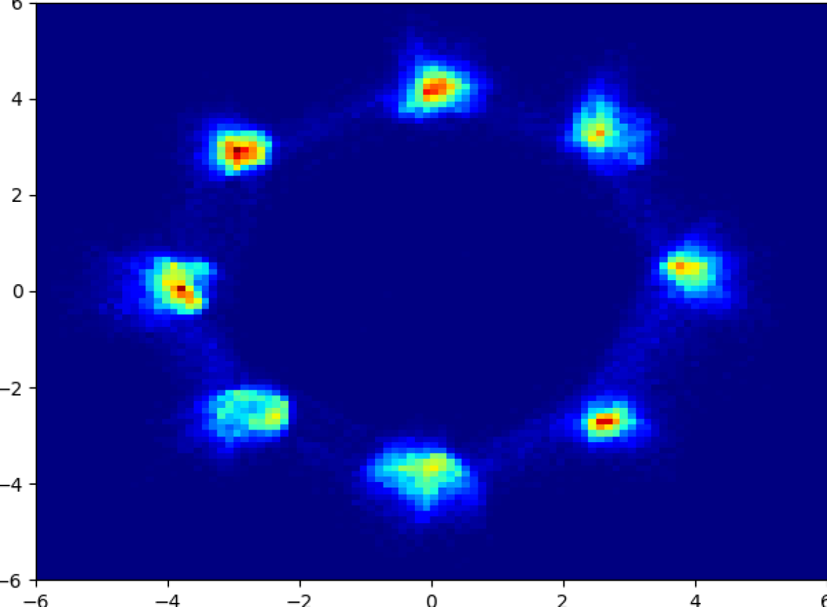
Figure 11(()): Mixture of Gaussian samples from GAN with the best hyperparameters from the heatmaps in Appendix Figure 10

Figure 11(()): Class-conditional CIFAR-10 samples from GAN with the best hyperparameters from the heatmap in C.4

Figure 12(()): The inception score (IS) for a grid search on $\arg(\beta_{1})$ and $|\beta_{1}|$ for training BigGAN on CIFAR-10 with the Adam variant in Algorithm 2. The $\beta_{1}$ is complex for the discriminator, while the generator’s optimizer is fixed to author-supplied defaults. Red points are runs that failed to train to the minimum IS in the color bar. The vertical magenta line denotes runs equivalent to alternating SGD. Negative momentum failed to train for any momentum magnitude $|\beta_{1}|>.5$, so we do not display it for more resolution near values of interest.

Figure 12(()): We compare the best optimization parameters from grid search Figure C.4 for our complex Adam variant (i.e., Algorithm 2) shown in green, with the author provided values shown in red for the CIFAR-10 BigGAN over $10$ seeds. A star is displayed at the best IS over all runs, a cross is displayed at the worst IS over all runs, while a circle is shown at the best IS for each run. Dashed lines are shown at the max/min IS over all runs at each iteration, low-alpha lines are shown for each runs IS, while solid lines are shown for the average IS over all seeds at each iteration. The results are summarized in Table 1.

References

- Goodfellow et al. [2014] Ian Goodfellow, Jean Pouget-Abadie, Mehdi Mirza, Bing Xu, David Warde-Farley, Sherjil Ozair, Aaron Courville, and Yoshua Bengio. Generative adversarial nets. In Advances in Neural Information Processing Systems, pages 2672–2680, 2014.
- Pfau and Vinyals [2016] David Pfau and Oriol Vinyals. Connecting generative adversarial networks and actor-critic methods. arXiv preprint arXiv:1610.01945, 2016.
- Baker et al. [2019] Bowen Baker, Ingmar Kanitscheider, Todor Markov, Yi Wu, Glenn Powell, Bob McGrew, and Igor Mordatch. Emergent tool use from multi-agent autocurricula. In International Conference on Learning Representations, 2019.
- Balduzzi et al. [2019] David Balduzzi, Marta Garnelo, Yoram Bachrach, Wojciech Czarnecki, Julien Perolat, Max Jaderberg, and Thore Graepel. Open-ended learning in symmetric zero-sum games. In International Conference on Machine Learning, pages 434–443. PMLR, 2019.
- Sukhbaatar et al. [2018] Sainbayar Sukhbaatar, Zeming Lin, Ilya Kostrikov, Gabriel Synnaeve, Arthur Szlam, and Rob Fergus. Intrinsic motivation and automatic curricula via asymmetric self-play. In International Conference on Learning Representations, 2018.
- Lorraine and Duvenaud [2018] Jonathan Lorraine and David Duvenaud. Stochastic hyperparameter optimization through hypernetworks. arXiv preprint arXiv:1802.09419, 2018.
- Lorraine et al. [2020] Jonathan Lorraine, Paul Vicol, and David Duvenaud. Optimizing millions of hyperparameters by implicit differentiation. In International Conference on Artificial Intelligence and Statistics, pages 1540–1552. PMLR, 2020.
- MacKay et al. [2019] Matthew MacKay, Paul Vicol, Jon Lorraine, David Duvenaud, and Roger Grosse. Self-tuning networks: Bilevel optimization of hyperparameters using structured best-response functions. In International Conference on Learning Representations (ICLR), 2019.
- Raghu et al. [2020] Aniruddh Raghu, Maithra Raghu, Simon Kornblith, David Duvenaud, and Geoffrey Hinton. Teaching with commentaries. arXiv preprint arXiv:2011.03037, 2020.
- Bose et al. [2020] Avishek Joey Bose, Gauthier Gidel, Hugo Berrard, Andre Cianflone, Pascal Vincent, Simon Lacoste-Julien, and William L Hamilton. Adversarial example games. arXiv preprint arXiv:2007.00720, 2020.
- Yuan et al. [2019] Xiaoyong Yuan, Pan He, Qile Zhu, and Xiaolin Li. Adversarial examples: Attacks and defenses for deep learning. IEEE Transactions on Neural Networks and Learning Systems, 30(9):2805–2824, 2019.
- Rajeswaran et al. [2020] Aravind Rajeswaran, Igor Mordatch, and Vikash Kumar. A game theoretic framework for model based reinforcement learning. arXiv preprint arXiv:2004.07804, 2020.
- Abachi et al. [2020] Romina Abachi, Mohammad Ghavamzadeh, and Amir-massoud Farahmand. Policy-aware model learning for policy gradient methods. arXiv preprint arXiv:2003.00030, 2020.
- Bacon et al. [2019] Pierre-Luc Bacon, Florian Schäfer, Clement Gehring, Animashree Anandkumar, and Emma Brunskill. A Lagrangian method for inverse problems in reinforcement learning. lis.csail.mit.edu/pubs, 2019.
- Acuna et al. [2021] David Acuna, Guojun Zhang, Marc T Law, and Sanja Fidler. f-domain-adversarial learning: Theory and algorithms for unsupervised domain adaptation with neural networks, 2021. URL https://openreview.net/forum?id=WqXAKcwfZtI.
- Grathwohl et al. [2018] Will Grathwohl, Elliot Creager, Seyed Kamyar Seyed Ghasemipour, and Richard Zemel. Gradient-based optimization of neural network architecture. 2018.
- Adam and Lorraine [2019] George Adam and Jonathan Lorraine. Understanding neural architecture search techniques. arXiv preprint arXiv:1904.00438, 2019.
- Ren et al. [2018] Mengye Ren, Eleni Triantafillou, Sachin Ravi, Jake Snell, Kevin Swersky, Joshua B Tenenbaum, Hugo Larochelle, and Richard S Zemel. Meta-learning for semi-supervised few-shot classification. arXiv preprint arXiv:1803.00676, 2018.
- Ren et al. [2020] Mengye Ren, Eleni Triantafillou, Kuan-Chieh Wang, James Lucas, Jake Snell, Xaq Pitkow, Andreas S Tolias, and Richard Zemel. Flexible few-shot learning with contextual similarity. arXiv preprint arXiv:2012.05895, 2020.
- Morgenstern and Von Neumann [1953] Oskar Morgenstern and John Von Neumann. Theory of Games and Economic Behavior. Princeton University Press, 1953.
- Von Stackelberg [2010] Heinrich Von Stackelberg. Market Structure and Equilibrium. Springer Science & Business Media, 2010.
- Berard et al. [2019] Hugo Berard, Gauthier Gidel, Amjad Almahairi, Pascal Vincent, and Simon Lacoste-Julien. A closer look at the optimization landscapes of generative adversarial networks. In International Conference on Learning Representations, 2019.
- Arrow et al. [1958] Kenneth Joseph Arrow, Hirofumi Azawa, Leonid Hurwicz, and Hirofumi Uzawa. Studies in Linear and Non-Linear Programming, volume 2. Stanford University Press, 1958.
- Freund and Schapire [1999] Yoav Freund and Robert E Schapire. Adaptive game playing using multiplicative weights. Games and Economic Behavior, 29(1-2):79–103, 1999.
- Gidel et al. [2019] Gauthier Gidel, Reyhane Askari Hemmat, Mohammad Pezeshki, Rémi Le Priol, Gabriel Huang, Simon Lacoste-Julien, and Ioannis Mitliagkas. Negative momentum for improved game dynamics. In The 22nd International Conference on Artificial Intelligence and Statistics, pages 1802–1811. PMLR, 2019.
- Lucas et al. [2018] James Lucas, Shengyang Sun, Richard Zemel, and Roger Grosse. Aggregated momentum: Stability through passive damping. In International Conference on Learning Representations, 2018.
- Polyak [1964] Boris T Polyak. Some methods of speeding up the convergence of iteration methods. USSR Computational Mathematics and Mathematical Physics, 4(5):1–17, 1964.
- Nesterov [1983] Yurii E Nesterov. A method for solving the convex programming problem with convergence rate o (1/k^ 2). In Dokl. Akad. Nauk SSSR, volume 269, pages 543–547, 1983.
- Sutskever et al. [2013] Ilya Sutskever, James Martens, George Dahl, and Geoffrey Hinton. On the importance of initialization and momentum in deep learning. In International Conference on Machine Learning, pages 1139–1147, 2013.
- Zhang and Wang [2020] Guodong Zhang and Yuanhao Wang. On the suboptimality of negative momentum for minimax optimization. arXiv preprint arXiv:2008.07459, 2020.
- Kingma and Ba [2014] Diederik P Kingma and Jimmy Ba. Adam: A method for stochastic optimization. arXiv preprint arXiv:1412.6980, 2014.
- Brock et al. [2018] Andrew Brock, Jeff Donahue, and Karen Simonyan. Large scale gan training for high fidelity natural image synthesis. In International Conference on Learning Representations, 2018.
- Osawa et al. [2019] Kazuki Osawa, Yohei Tsuji, Yuichiro Ueno, Akira Naruse, Rio Yokota, and Satoshi Matsuoka. Large-scale distributed second-order optimization using kronecker-factored approximate curvature for deep convolutional neural networks. In Proceedings of the IEEE/CVF Conference on Computer Vision and Pattern Recognition, pages 12359–12367, 2019.
- Mescheder et al. [2017] Lars Mescheder, Sebastian Nowozin, and Andreas Geiger. The numerics of GANs. In Advances in Neural Information Processing Systems, pages 1825–1835, 2017.
- Schäfer and Anandkumar [2019] Florian Schäfer and Anima Anandkumar. Competitive gradient descent. In Advances in Neural Information Processing Systems, pages 7623–7633, 2019.
- Wang et al. [2019] Yuanhao Wang, Guodong Zhang, and Jimmy Ba. On solving minimax optimization locally: A follow-the-ridge approach. In International Conference on Learning Representations, 2019.
- Hemmat et al. [2020] Reyhane Askari Hemmat, Amartya Mitra, Guillaume Lajoie, and Ioannis Mitliagkas. Lead: Least-action dynamics for min-max optimization. arXiv preprint arXiv:2010.13846, 2020.
- Schäfer et al. [2020] Florian Schäfer, Anima Anandkumar, and Houman Owhadi. Competitive mirror descent. arXiv preprint arXiv:2006.10179, 2020.
- Czarnecki et al. [2020] Wojciech Marian Czarnecki, Gauthier Gidel, Brendan Tracey, Karl Tuyls, Shayegan Omidshafiei, David Balduzzi, and Max Jaderberg. Real world games look like spinning tops. arXiv preprint arXiv:2004.09468, 2020.
- Zhang et al. [2020a] Guojun Zhang, Kaiwen Wu, Pascal Poupart, and Yaoliang Yu. Newton-type methods for minimax optimization. arXiv preprint arXiv:2006.14592, 2020a.
- Korpelevich [1976] GM Korpelevich. The extragradient method for finding saddle points and other problems. Matecon, 12:747–756, 1976.
- Mescheder et al. [2018] Lars Mescheder, Andreas Geiger, and Sebastian Nowozin. Which training methods for gans do actually converge? In International Conference on Machine learning (ICML), pages 3481–3490. PMLR, 2018.
- Harris et al. [2020] Charles R Harris, K Jarrod Millman, Stéfan J van der Walt, Ralf Gommers, Pauli Virtanen, David Cournapeau, Eric Wieser, Julian Taylor, Sebastian Berg, Nathaniel J Smith, et al. Array programming with numpy. Nature, 585(7825):357–362, 2020.
- Bertsekas [2008] D Bertsekas. Nonlinear Programming. Athena Scientific, 2008.
- O’donoghue and Candes [2015] Brendan O’donoghue and Emmanuel Candes. Adaptive restart for accelerated gradient schemes. Foundations of computational mathematics, 15(3):715–732, 2015.
- Goh [2017] Gabriel Goh. Why momentum really works. Distill, 2(4):e6, 2017.
- Azizian et al. [2020a] Waïss Azizian, Ioannis Mitliagkas, Simon Lacoste-Julien, and Gauthier Gidel. A tight and unified analysis of gradient-based methods for a whole spectrum of differentiable games. In International Conference on Artificial Intelligence and Statistics, pages 2863–2873. PMLR, 2020a.
- Bradbury et al. [2018] James Bradbury, Roy Frostig, Peter Hawkins, Matthew James Johnson, Chris Leary, Dougal Maclaurin, and Skye Wanderman-Milne. JAX: composable transformations of Python+NumPy programs, 2018. URL http://github.com/google/jax.
- Paszke et al. [2017] Adam Paszke, Sam Gross, Soumith Chintala, Gregory Chanan, Edward Yang, Zachary DeVito, Zeming Lin, Alban Desmaison, Luca Antiga, and Adam Lerer. Automatic differentiation in PyTorch. Openreview, 2017.
- Chiang et al. [2012] Chao-Kai Chiang, Tianbao Yang, Chia-Jung Lee, Mehrdad Mahdavi, Chi-Jen Lu, Rong Jin, and Shenghuo Zhu. Online optimization with gradual variations. In Conference on Learning Theory, pages 6–1. JMLR Workshop and Conference Proceedings, 2012.
- Rakhlin and Sridharan [2013] Alexander Rakhlin and Karthik Sridharan. Optimization, learning, and games with predictable sequences. In Proceedings of the 26th International Conference on Neural Information Processing Systems-Volume 2, pages 3066–3074, 2013.
- Daskalakis et al. [2018] Constantinos Daskalakis, Andrew Ilyas, Vasilis Syrgkanis, and Haoyang Zeng. Training gans with optimism. In International Conference on Learning Representations (ICLR 2018), 2018.
- Wu et al. [2019] Yan Wu, Jeff Donahue, David Balduzzi, Karen Simonyan, and Timothy Lillicrap. Logan: Latent optimisation for generative adversarial networks. arXiv preprint arXiv:1912.00953, 2019.
- Krizhevsky [2009] Alex Krizhevsky. Learning multiple layers of features from tiny images. Technical report, University of Toronto, 2009.
- Nesterov [2013] Yurii Nesterov. Introductory lectures on convex optimization: A basic course, volume 87. Springer Science & Business Media, 2013.
- Maddison et al. [2018] Chris J Maddison, Daniel Paulin, Yee Whye Teh, Brendan O’Donoghue, and Arnaud Doucet. Hamiltonian descent methods. arXiv preprint arXiv:1809.05042, 2018.
- Zhang and Mitliagkas [2017] Jian Zhang and Ioannis Mitliagkas. Yellowfin and the art of momentum tuning. arXiv preprint arXiv:1706.03471, 2017.
- Choi et al. [2019] Dami Choi, Christopher J Shallue, Zachary Nado, Jaehoon Lee, Chris J Maddison, and George E Dahl. On empirical comparisons of optimizers for deep learning. arXiv preprint arXiv:1910.05446, 2019.
- Zhang et al. [2019] Michael R Zhang, James Lucas, Geoffrey Hinton, and Jimmy Ba. Lookahead optimizer: k steps forward, 1 step back. arXiv preprint arXiv:1907.08610, 2019.
- Chen et al. [2020] Ricky TQ Chen, Dami Choi, Lukas Balles, David Duvenaud, and Philipp Hennig. Self-tuning stochastic optimization with curvature-aware gradient filtering. arXiv preprint arXiv:2011.04803, 2020.
- Foerster et al. [2018] Jakob Foerster, Richard Y Chen, Maruan Al-Shedivat, Shimon Whiteson, Pieter Abbeel, and Igor Mordatch. Learning with opponent-learning awareness. In International Conference on Autonomous Agents and MultiAgent Systems, pages 122–130, 2018.
- Maclaurin et al. [2015] Dougal Maclaurin, David Duvenaud, and Ryan Adams. Gradient-based hyperparameter optimization through reversible learning. In International Conference on Machine Learning, pages 2113–2122, 2015.
- Letcher et al. [2019] Alistair Letcher, David Balduzzi, Sébastien Racaniere, James Martens, Jakob N Foerster, Karl Tuyls, and Thore Graepel. Differentiable game mechanics. Journal of Machine Learning Research, 20(84):1–40, 2019.
- Nagarajan et al. [2020] Sai Ganesh Nagarajan, David Balduzzi, and Georgios Piliouras. From chaos to order: Symmetry and conservation laws in game dynamics. In International Conference on Machine Learning, pages 7186–7196. PMLR, 2020.
- Omidshafiei et al. [2020] Shayegan Omidshafiei, Karl Tuyls, Wojciech M Czarnecki, Francisco C Santos, Mark Rowland, Jerome Connor, Daniel Hennes, Paul Muller, Julien Pérolat, Bart De Vylder, et al. Navigating the landscape of multiplayer games. Nature communications, 11(1):1–17, 2020.
- Gidel et al. [2020] Gauthier Gidel, David Balduzzi, Wojciech Marian Czarnecki, Marta Garnelo, and Yoram Bachrach. Minimax theorem for latent games or: How i learned to stop worrying about mixed-nash and love neural nets. arXiv preprint arXiv:2002.05820, 2020.
- Perolat et al. [2020] Julien Perolat, Remi Munos, Jean-Baptiste Lespiau, Shayegan Omidshafiei, Mark Rowland, Pedro Ortega, Neil Burch, Thomas Anthony, David Balduzzi, Bart De Vylder, et al. From poincar’e recurrence to convergence in imperfect information games: Finding equilibrium via regularization. arXiv preprint arXiv:2002.08456, 2020.
- Zhang et al. [2021] Guodong Zhang, Yuanhao Wang, Laurent Lessard, and Roger Grosse. Don’t fix what ain’t broke: Near-optimal local convergence of alternating gradient descent-ascent for minimax optimization. arXiv preprint arXiv:2102.09468, 2021.
- Zhang et al. [2020b] Guodong Zhang, Xuchao Bao, Laurent Lessard, and Roger Grosse. A unified analysis of first-order methods for smooth games via integral quadratic constraints. arXiv preprint arXiv:2009.11359, 2020b.
- Ibrahim et al. [2020] Adam Ibrahim, Waıss Azizian, Gauthier Gidel, and Ioannis Mitliagkas. Linear lower bounds and conditioning of differentiable games. In International Conference on Machine Learning, pages 4583–4593. PMLR, 2020.
- Bailey et al. [2020] James P Bailey, Gauthier Gidel, and Georgios Piliouras. Finite regret and cycles with fixed step-size via alternating gradient descent-ascent. In Conference on Learning Theory, pages 391–407. PMLR, 2020.
- Jin et al. [2020] Chi Jin, Praneeth Netrapalli, and Michael Jordan. What is local optimality in nonconvex-nonconcave minimax optimization? In International Conference on Machine Learning, pages 4880–4889. PMLR, 2020.
- Nouiehed et al. [2019] Maher Nouiehed, Maziar Sanjabi, Tianjian Huang, Jason D Lee, and Meisam Razaviyayn. Solving a class of non-convex min-max games using iterative first order methods. Advances in Neural Information Processing Systems, 32:14934–14942, 2019.
- Zhang et al. [2020c] Guojun Zhang, Pascal Poupart, and Yaoliang Yu. Optimality and stability in non-convex smooth games. arXiv e-prints, pages arXiv–2002, 2020c.
- Azizian et al. [2020b] Waïss Azizian, Damien Scieur, Ioannis Mitliagkas, Simon Lacoste-Julien, and Gauthier Gidel. Accelerating smooth games by manipulating spectral shapes. arXiv preprint arXiv:2001.00602, 2020b.
- Domingo-Enrich et al. [2020] Carles Domingo-Enrich, Fabian Pedregosa, and Damien Scieur. Average-case acceleration for bilinear games and normal matrices. arXiv preprint arXiv:2010.02076, 2020.
- Zhang and Yu [2019] Guojun Zhang and Yaoliang Yu. Convergence of gradient methods on bilinear zero-sum games. In International Conference on Learning Representations, 2019.
- Loizou et al. [2020] Nicolas Loizou, Hugo Berard, Alexia Jolicoeur-Martineau, Pascal Vincent, Simon Lacoste-Julien, and Ioannis Mitliagkas. Stochastic hamiltonian gradient methods for smooth games. In International Conference on Machine Learning, pages 6370–6381. PMLR, 2020.
- Liu et al. [2020] Mingrui Liu, Youssef Mroueh, Jerret Ross, Wei Zhang, Xiaodong Cui, Payel Das, and Tianbao Yang. Towards better understanding of adaptive gradient algorithms in generative adversarial nets. In International Conference on Learning Representations, 2020. URL https://openreview.net/forum?id=SJxIm0VtwH.
- Peng et al. [2020] Wei Peng, Yu-Hong Dai, Hui Zhang, and Lizhi Cheng. Training gans with centripetal acceleration. Optimization Methods and Software, 35(5):955–973, 2020.
- Albuquerque et al. [2019] Isabela Albuquerque, João Monteiro, Thang Doan, Breandan Considine, Tiago Falk, and Ioannis Mitliagkas. Multi-objective training of generative adversarial networks with multiple discriminators. In International Conference on Machine Learning, pages 202–211. PMLR, 2019.
- Hsieh et al. [2019] Ya-Ping Hsieh, Chen Liu, and Volkan Cevher. Finding mixed nash equilibria of generative adversarial networks. In International Conference on Machine Learning, pages 2810–2819. PMLR, 2019.
- Metz et al. [2016] Luke Metz, Ben Poole, David Pfau, and Jascha Sohl-Dickstein. Unrolled generative adversarial networks. arXiv preprint arXiv:1611.02163, 2016.
- Qin et al. [2020] Chongli Qin, Yan Wu, Jost Tobias Springenberg, Andrew Brock, Jeff Donahue, Timothy P Lillicrap, and Pushmeet Kohli. Training generative adversarial networks by solving ordinary differential equations. arXiv preprint arXiv:2010.15040, 2020.
- Schäfer et al. [2019] Florian Schäfer, Hongkai Zheng, and Anima Anandkumar. Implicit competitive regularization in gans. arXiv preprint arXiv:1910.05852, 2019.
- Jolicoeur-Martineau and Mitliagkas [2019] Alexia Jolicoeur-Martineau and Ioannis Mitliagkas. Connections between support vector machines, wasserstein distance and gradient-penalty gans. arXiv preprint arXiv:1910.06922, 2019.
- Gidel et al. [2018] Gauthier Gidel, Hugo Berard, Gaëtan Vignoud, Pascal Vincent, and Simon Lacoste-Julien. A variational inequality perspective on generative adversarial networks. In International Conference on Learning Representations, 2018.
- Chavdarova et al. [2019] Tatjana Chavdarova, Gauthier Gidel, Francois Fleuret, and Simon Lacoste-Julien. Reducing noise in gan training with variance reduced extragradient. In Proceedings of the international conference on Neural Information Processing Systems, number CONF, 2019.
- Salimans et al. [2016] Tim Salimans, Ian Goodfellow, Wojciech Zaremba, Vicki Cheung, Alec Radford, and Xi Chen. Improved techniques for training GANs. In Advances in Neural Information Processing Systems, pages 2234–2242, 2016.
- Foucart [2012] Simon Foucart. Matrix norm and spectral radius. https://www.math.drexel.edu/~foucart/TeachingFiles/F12/M504Lect6.pdf, 2012. Accessed: 2020-05-21.
- Boyd et al. [2004] Stephen Boyd, Stephen P Boyd, and Lieven Vandenberghe. Convex optimization. Cambridge university press, 2004.
- Hahnloser et al. [2000] Richard HR Hahnloser, Rahul Sarpeshkar, Misha A Mahowald, Rodney J Douglas, and H Sebastian Seung. Digital selection and analogue amplification coexist in a cortex-inspired silicon circuit. Nature, 405(6789):947–951, 2000.