Unveiling the $K_{1}(1270)$ double-pole structure in the $\bar{B}\to J/\psi\rho\bar{K}$ and $\bar{B}\to J/\psi\bar{K}^{*}\pi$ decays

Abstract

By looking at the pseudoscalar-vector meson spectra in the $\bar{B}\to J/\psi\rho\bar{K}$ and $\bar{B}\to J/\psi\bar{K}^{*}\pi$ weak decays, we theoretically investigate the double-pole structure of the $K_{1}(1270)$ resonance by using the Chiral Unitary approach to account for the final state interactions between the pseudoscalar $(P)$ and vector ($V$) mesons. The $K_{1}(1270)$ resonance is dynamically generated through these interactions in coupled channels and influences the shape of the invariant mass distributions under consideration. We show how these shapes are affected by the $K_{1}(1270)$ double-pole structure to confront the results from our model with future experiments that might investigate the $PV$ spectra in these decays.

I Introduction

The observation of the axial vector mesons $K_{1}(1270)$ and $K_{1}(1400)$ Brandenburg:1975gv ; daum were identified as the expected $1^{+}$ strange mesons from the quark model. Subsequent experiments have explored their properties and decay modes pdg . While the dominant $K_{1}(1270)$ decay channel is $\rho K$, the $K_{1}(1400)$ is observed to decay mostly through the $K^{*}(892)\pi$ one. These states have usually been studied in terms of the mixing of the strange states of the $J^{PC}=1^{++}$ and $J^{PC}=1^{+-}$ nonets (see for example Suzuki:1993yc ; Tayduganov:2011ui ; Zhang:2017cbi ). Other exhaustive analyses of the $1^{+}$ low-lying mesons as dynamically generated resonances found that the $S=1$ and $I=1/2$ poles were not compatible with the above assignment, but rather they should be identified as a double-pole structure for the $K_{1}(1270)$ Roca:2005nm . The two pole structure for the $K_{1}(1270)$ resonance is not unique: there are several cases where two poles were found for hadronic resonances, and a recent review can be seen in Ref. ulfreview . The discovery of the two-pole structure of the $K_{1}(1270)$ triggered studies looking for scenarios where this prediction could be tested. The analysis of the $K^{-}p\to K^{-}\pi^{+}\pi^{-}p$ data at $63$ GeV done in Ref. daum provided additional support to the existence of two states: one with a mass of 1195 MeV coupling mostly to the $K^{*}(892)\pi$ channel, and one with a mass of 1284 MeV coupling to the $\rho K$ one. Several reactions aimed at observing these two states were proposed, such as $D^{0}\to\pi^{+}VP$ wang2019 , which is similar to $B^{-}\to J/\psi K^{-}_{1}(1270)$ with the hadronization involving three light mesons. More recently, another study considered the $D^{+}\to\nu\l^{+}K_{1}(1270)$ decay wang2020 , identifying the signatures in the invariant-mass distributions of the decaying $K_{1}(1270)$. On the other hand, expected improvements in the experimental capabilities to study $B$-meson decays with higher statistics, like in the Belle II experiment, make these proposals an interesting scenario to look for.

In this work we provide an additional reaction, considering decays of the form $\bar{B}^{0}\to J/\psi VP$, where $VP$ are the vector and pseudoscalar meson pairs, $\rho\bar{K}$ and $\bar{K}^{*}\pi$, using the chiral unitary approach, and we look for signatures of the two $K_{1}(1270)$ states. A related work was done in wangzhang , where the reaction $B^{-}\rightarrow J/\psi\rho^{0}K^{-}$ was studied to look for signals of the $Z_{c}(4000)$; however, simultaneously one $K_{1}(1270)$ showed up in the $\rho\bar{K}$ mass distribution. Here we also look into the $\bar{K}^{*}\pi$ channel in order to see both $K_{1}(1270)$ states.

The work proceeds as follows: In section II, we present the formalism for the elementary production at the quark level, where the different $VP$ channels are related by $SU(3)$ arguments. Then, we account for the final $VP$ interaction by implementing meson-meson scattering based on the Chiral Unitary approach. In section III we compute the invariant-mass distribution for the $VP$ pair and its structure in terms of the individual poles, and identify the regions where the signature of such poles can be extracted.

II Formalism

II.1 $VP$ pseudoscalar and vector mesons production

The relevant contribution for the $\bar{B}\to J/\psi\,VP$ reaction is given at the quark level by the diagram shown in Fig. 1.

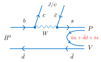
Figure 1: Dominant diagram for the $\bar{B}\to J/\psi(P\,V)$ reaction at the quark level. In the first step, a $b$ quark decays into a $c$ one by emission of a gauge boson $W$ which then produces a strange quark $s$ along with a $\bar{c}$ one. Finally, we are left with a $c\bar{c}$ pair, forming the $J/\psi$, and the $s\bar{d}$ one. This latter pair is hadronized in order to produce a pseudoscalar-vector meson pair emerging as the final state.

The mechanism starts with a $b\bar{d}$ quark pair, forming the initial $\bar{B}^{0}$ meson, in which the $b$ quark is converted into a $c$ quark by emitting a $W$ boson, which then produces an anticharm $\bar{c}$ along with a strange quark $s$. In the end, we are left with a $c\bar{c}$ pair making up a $J/\psi$ meson, considered as a spectator, and a $s\bar{d}$ pair. In order to produce a pseudoscalar as well as a vector meson, a $\bar{q}q$ pair with the quantum numbers of the vacuum is added to the already existing $s\bar{d}$ pair, according to the ${}^{3}P_{0}$ model hadro1 ; hadro2 ; hadro3 . Therefore, the final meson-meson hadronic state has the following quark flavor combination:

$$|H\rangle=|s(\bar{u}u+\bar{d}d+\bar{s}s)\bar{d}\rangle\,.$$ (1)

However, Eq. (1) above only refers to the quark content of the final mesonic states and it does not carry any information about the pseudoscalar or vector nature of those hadronic states. This is done by defining the $q\bar{q}$-matrix denoted as $M$, written as

$$M=\left(\begin{array}[]{ccc}u\bar{u}&u\bar{d}&u\bar{s}\\ d\bar{u}&d\bar{d}&d\bar{s}\\ s\bar{u}&s\bar{d}&s\bar{s}\end{array}\right)\,,$$ (2)

in terms of which Eq. (1) reads

$$|H\rangle=|s(\bar{u}u+\bar{d}d+\bar{s}s)\bar{d}\rangle=\sum_{i}|s\,\bar{q}_{i}\,q_{i}\,\bar{d}\rangle=|M_{3i}\,M_{i2}\rangle=|(MM)_{32}\rangle\,.$$ (3)

The final meson-meson components are found by establishing the correspondence between $M$ and the pseudoscalar and vector meson $SU(3)$ matrices, that is

$$M\Rightarrow P=\left(\begin{array}[]{ccc}\frac{\pi^{0}}{\sqrt{2}}+\frac{\eta}{\sqrt{3}}+\frac{\eta^{\prime}}{\sqrt{6}}&\pi^{+}&K^{+}\\ \pi^{-}&-\frac{\pi^{0}}{\sqrt{2}}+\frac{\eta}{\sqrt{3}}+\frac{\eta^{\prime}}{\sqrt{6}}&K^{0}\\ K^{-}&\bar{K}^{0}&-\frac{1}{\sqrt{3}}\eta+\sqrt{\frac{2}{3}}\eta^{\prime}\\ \end{array}\right),$$ (4)

and

$$M\Rightarrow V=\left(\begin{array}[]{ccc}\frac{\rho^{0}}{\sqrt{2}}+\frac{\omega}{\sqrt{2}}&\rho^{+}&K^{*+}\\ \rho^{-}&-\frac{\rho^{0}}{\sqrt{2}}+\frac{\omega}{\sqrt{2}}&K^{*0}\\ K^{*-}&\bar{K}^{*0}&\phi\\ \end{array}\right)\,,$$ (5)

where the standard $\eta-\eta^{\prime}$ bramon and $\omega_{1}-\omega_{8}$ mixings have been used for $P$ and $V$, respectively, in order to match the right flavor content of the matrix $M$.

Since we aim at describing a reaction with a pseudoscalar along with a vector meson as final states, the matrix $M$ in Eqs. (4) and (5) should be combined according to Eq. (3) in such a way that it gives the product $PV$ or $VP$. There is nothing in our model that privileges one over the other, and thus we consider an equal-weighted combination between them in Eq. (3) so that it can be rewritten as

$$|H\rangle=|(PV)_{32}\rangle+|(VP)_{32}\rangle\,.$$ (6)

Therefore, the pseudoscalar and vector mesons produced in the reaction are

$$|H\rangle=|\,\rho^{+}\bar{K}^{-}\,\rangle-\frac{1}{\sqrt{2}}|\,\rho^{0}\bar{K}^{0}\,\rangle+|\,K^{*-}\pi^{+}\,\rangle-\frac{1}{\sqrt{2}}|\,\bar{K}^{*0}\pi^{0}\,\rangle+\frac{1}{\sqrt{2}}|\,\omega\bar{K}^{0}\,\rangle+|\,\phi\bar{K}^{0}\,\rangle\,\,,$$ (7)

where a term corresponding to the $\bar{K}^{*0}\eta$ channel has canceled out in the evaluation of Eq. (6) by using Eqs. (4) and (5). Note that the procedure adopted provides the final $VP$ meson-meson components as well as their relative weights, which will play a significant role in the mass spectrum.

The final $|H\rangle$ state can be written in the isospin basis by considering the following multiplets: $(-\rho^{+},\rho^{0},\rho^{-})$, $(\bar{K}^{0},-K^{-})$, $(-\pi^{+},\pi^{0},\pi^{-})$ for the $\rho$, $\bar{K}$ and $\pi$ mesons, respectively. Then, the final $VP$ states in isospin $I=1/2$ are given by

$$|\,\rho\,\bar{K}\,\rangle_{I_{3}=1/2}^{I=1/2} = \sqrt{\frac{2}{3}}\,|\,\rho^{+}K^{-}\,\rangle-\sqrt{\frac{1}{3}}\,|\,\rho^{0}\bar{K}^{0}\,\rangle\,,$$

$$|\,\bar{K}^{*}\,\pi\,\rangle_{I_{3}=1/2}^{I=1/2} = -\sqrt{\frac{2}{3}}\,|\,K^{*-}\pi^{+}\,\rangle+\sqrt{\frac{1}{3}}\,|\,\bar{K}^{*0}\pi^{0}\,\rangle\,.$$ (8)

Using this, we can recast $|H\rangle$ as

$$|H\rangle=\sqrt{\frac{3}{2}}\,|\,\rho\,\bar{K}\,\rangle_{I_{3}=1/2}^{I=1/2}-\sqrt{\frac{3}{2}}\,|\,\bar{K}^{*}\,\pi\,\rangle_{I_{3}=1/2}^{I=1/2}+\frac{1}{\sqrt{2}}\,|\,\omega\bar{K}\,\rangle_{I_{3}=1/2}^{I=1/2}+|\,\phi\bar{K}\,\rangle_{I_{3}=1/2}^{I=1/2}\,.$$ (9)

This last equation also provides the relative weights, denoted as $h_{i}$, in the isospin basis between the $i$th $VP$ channels above. They are

$$h_{\rho\bar{K}} =\sqrt{\frac{3}{2}}; h_{\bar{K}^{*}\pi} =-\sqrt{\frac{3}{2}}\,;$$

$$h_{\omega\bar{K}} =\frac{1}{\sqrt{2}}; h_{\phi\bar{K}} =1\,.$$ (10)

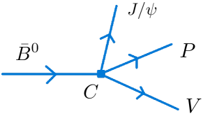
Figure 2: Amplitude for the $\bar{B}\to J/\psi(PV)$ decay. The $C$ constant is the parametrization of the weak vertex.

The differential decay width for the $\bar{B}\to J/\psi(PV)$ process, illustrated in Fig. 2, is given by

$$\frac{d\Gamma}{dM_{inv}}=\frac{1}{(2\pi)^{3}}\frac{1}{4M^{2}_{B}}p_{J/\psi}\tilde{p}_{\pi(\bar{K})}|T_{B\to J/\psi(PV)}|^{2}\,,$$ (11)

where $M_{B}$ is the $\bar{B}$-meson mass while $p_{J/\psi}$ and $\tilde{p}_{\pi(\bar{K})}$ are the momentum associated with $J/\psi$ in the $\bar{B}$ rest frame and $\pi(\bar{K})$ mesons in the $PV$ rest frame, respectively. As a function of the $PV$ invariant mass, $M_{inv}$, they are

$$p_{J/\psi}=\frac{\lambda^{1/2}(M^{2}_{B},M^{2}_{J/\psi},M^{2}_{inv})}{2M_{B}}\,,$$ (12)

$$\tilde{p}_{\bar{K}}=\frac{\lambda^{1/2}(M^{2}_{inv},M^{2}_{\rho},m^{2}_{\bar{K}})}{2M_{inv}}\,\,\textrm{for the}\,\,\rho\bar{K}\,\,\textrm{channel}\,,$$ (13)

$$\tilde{p}_{\pi}=\frac{\lambda^{1/2}(M^{2}_{inv},M^{2}_{\bar{K}^{*}},m^{2}_{\pi})}{2M_{inv}}\,\,\textrm{for the}\,\,\bar{K}^{*}\pi\,\,\textrm{channel}\,,$$ (14)

where $\lambda$ stands for the Källén function.

For the evaluation of the full decay amplitude, which is needed in Eq. (11), we have to consider the diagrams in Fig. 3, where the final-state interaction mechanism is implemented to take into account the $K_{1}(1270)$ resonance contribution for the invariant-mass spectra we are interested in. Since we are interested in the distributions with $\rho\bar{K}$ and $\bar{K}^{*}\pi$ as final $VP$ states, we have

$$T_{\bar{B}\to J/\psi\rho\bar{K}}=C\,(\vec{\epsilon}_{\psi}\cdot\vec{\epsilon}_{\rho})\Big{(}h_{\rho\bar{K}}+\sum_{i}\,h_{i}\,G_{i}(M_{inv})\,t^{I=1/2}_{i\to\rho\bar{K}}(M_{inv})\Big{)}\,,$$ (15)

and

$$T_{\bar{B}\to J/\psi\bar{K}^{*}\pi}=C\,(\vec{\epsilon}_{\psi}\cdot\vec{\epsilon}_{\bar{K}^{*}})\Big{(}h_{\bar{K}^{*}\pi}+\sum_{i}\,h_{i}\,G_{i}(M_{inv})\,t^{I=1/2}_{i\to\bar{K}^{*}\pi}(M_{inv})\Big{)}\,,$$ (16)

where the index $i$, running from $1$ to $4$, stands for each possible $VP$ channel involved in the loop, and $C$ contains the information of the strength of the weak decay at the tree-level. The channels are: $i=1$ for $\phi\bar{K}$, $i=2$ for $\omega\bar{K}$, $i=3$ for $\rho\bar{K}$, $i=4$ for $\bar{K}^{*}\pi$. These loops are represented by $G_{i}(M_{inv})$ which is the $G$-loop function (given as a function of the invariant mass $M_{inv}$) which we will discuss in Subsection II.2. The $h_{i}$’s are the relative weights in the isospin basis, defined in Eq. (II.1) above. Moreover, $\vec{\epsilon}_{\psi}$, $\vec{\epsilon}_{\rho}$, $\vec{\epsilon}_{\bar{K}^{*}}$ are the polarization vectors for the $J/\psi$, $\rho$, and $\bar{K}^{*}$ mesons, respectively.

Furthermore, the amplitudes $t^{I=1/2}_{i\to\rho\bar{K}}$ and $t^{I=1/2}_{i\to\bar{K}^{*}\pi}$ in Eqs. (15) and (16) are the two-body scattering amplitudes for all possible transitions from the $i$th channel to $\rho\bar{K}$ (and to $\bar{K}^{*}\pi$), which in our approach encode the resonance $K_{1}(1270)$ as dynamically generated through these interactions geng2007 , and are explained in the following subsection.

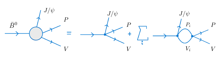
Figure 3: Relevant diagrams contributing to the amplitude $T_{\bar{B}\to J/\psi(PV)}$ implementing the final state interaction. The first diagram on the right-hand side corresponds to the tree-level. On the other hand, the second one with a loop encodes the final state interaction mechanism and, actually it is a sum over all $P_{i}V_{i}$ pseudoscalar and vector mesons associated with the $i$-channel: $i=1$ for $\phi\bar{K}$, $i=2$ for $\omega\bar{K}$, $i=3$ for $\rho\bar{K}$, $i=4$ for $\bar{K}^{*}\pi$.

II.2 Final-state interaction and the $K_{1}(1270)$ resonance

Once the final meson-meson pair is produced at tree-level in the $\bar{B}\to J/\psi\,VP$ reaction, they undergo final-state interaction from which the $K_{1}(1270)$ resonance emerges dynamically. In fact, in Ref. geng2007 this resonance was dynamically generated through the $s$-wave interaction between the pseudoscalar and vector mesons in the $I=1/2$ channel. The final-state interaction mechanism is introduced by adopting a unitarization procedure using the Bethe-Salpeter equation in coupled channels, from which some hadronic states show up as poles in the unphysical Riemann sheets of the scattering matrices. This approach is a unitary extension of Chiral Perturbation theory, called the Chiral Unitary approach oller1 ; oller2 ; oller3 , which has allowed to describe many hadronic resonances as composite states of mesons and/or baryons. In particular, in Ref. geng2007 the transition amplitudes $t^{I=1/2}_{i\to j}$ appearing in Eqs. (15) and (16) were unitarized by solving a coupled-channel scattering equation in an algebraic form, written in matrix form as

$$t=(1-V\,G)^{-1}V\,,$$ (17)

where in $V_{ij}$, $t_{ij}$ the indices stand for the coupled channels: $1$ for $\phi\bar{K}$, $2$ for $\omega\bar{K}$, $3$ for $\rho\bar{K}$, $4$ for $\bar{K}^{*}\pi$ and $5$ for $\bar{K}^{*}\eta$. In addition, $V_{ij}$ is the interaction kernel, which corresponds to the tree-level amplitudes evaluated for all channels we are considering in this work by using the chiral Lagrangians from Ref. Birse given by

$$\mathcal{L}_{VVPP}=-\frac{1}{4f^{2}}\,\textrm{Tr}\,\Big{(}\,[V^{\mu},\partial^{\nu}V_{\mu}]\,[P,\partial_{\nu}P]\,\Big{)}\,,$$ (18)

with $f$ the pion decay constant ($f=93$ MeV) and $V,P$ are the matrices given in Eqs. (4) and (5). Furthermore, $G_{k}(s)$ is the meson-meson loop function associated to the $k$th channel, which can be regularized either by dimensional or cutoff regularization schemes. In the present work, we follow Ref. geng2007 which employs the former scheme. In this case, the $G_{k}(s)$ loop function is given by

$$G_{k}(\sqrt{s}) = \frac{1}{16\pi^{2}}\Big{\{}a(\mu)+ln\frac{M^{2}_{k}}{\mu^{2}}+\frac{m^{2}_{k}-M^{2}_{k}+s}{2s}ln\frac{m^{2}_{k}}{M^{2}_{k}}+\frac{q_{k}}{\sqrt{s}}[ln(s-(M^{2}_{k}-m^{2}_{k})+2q_{k}\sqrt{s})$$ (19)

$$+ ln(s+(M^{2}_{k}-m^{2}_{k})+2q_{k}\sqrt{s})-ln(-s+(M^{2}_{k}-m^{2}_{k})+2q_{k}\sqrt{s})$$

$$- ln(-s-(M^{2}_{k}-m^{2}_{k})+2q_{k}\sqrt{s})]\Big{\}}\,,$$

where $M_{k}$ and $m_{k}$ stand for the vector and pseudoscalar meson masses in the $k$th channel, respectively. Moreover, $a(\mu)$ is the subtraction constant and in this work we take $a(\mu)=-1.85$ for $\mu=900$ MeV, which is the scale of dimensional regularization, obtained in Ref. geng2007 by fitting the experimental $K^{-}p\to K^{-}\pi^{+}\pi^{-}p$ data. In addition, $q_{k}=|\vec{q}_{k}|$ is the on-shell three-momentum of the meson in the loop, given in the center of mass frame by

$$q_{k}=\frac{\lambda^{1/2}(s,M^{2}_{k},m^{2}_{k})}{2\sqrt{s}}\,.$$ (20)

The $\rho$ and $\bar{K}^{*}$ mesons have a relatively large width and hence a wide mass distribution. In order to take this feature into account in our formalism, we convolve the loop function $G_{k}(s)$ with the corresponding vector meson spectral function

$$\textrm{Im}[D(s_{V})]=\textrm{Im}\Big{(}\frac{1}{s_{V}-M_{V}^{2}+iM_{V}\Gamma_{V}}\Big{)}\,,$$ (21)

where $M_{V}$ stands for the vector meson mass and $\Gamma_{V}$ is the vector meson width, considered here as energy independent. Choosing an energy-dependent form for $\Gamma_{V}$, as was done in Refs. wang2019 ; wang2020 , does not provide any significant change in our results compared with the usual uncertainties of our approach. The spectral function above is related to the exact propagator for the vector meson by using the Lehmann representation, which gives us

$$D(s)=-\frac{1}{\pi}\int\limits_{s_{th}}^{\infty}\,ds_{V}\,\frac{\textrm{Im}[D(s_{V})]}{s-s_{V}+i\epsilon}\,,$$ (22)

with $s_{th}$ the corresponding vector meson threshold for the decay channels with the $\rho$ or $\bar{K}^{*}$ mesons. Therefore, the convolution of the $G_{k}(s)$ loop function defined in Eq. (19) with the vector meson spectral function given by Eq. (22) provides

$$G(\sqrt{s},M_{k},m_{k})=\frac{\int\limits_{(M_{V}-2\Gamma_{V})^{2}}^{(M_{V}+2\Gamma_{V})^{2}}\,ds_{V}\,G(\sqrt{s},\sqrt{s_{V}},m_{k})\times\textrm{Im}[D(s_{V})]}{\int\limits_{(M_{V}-2\Gamma_{V})^{2}}^{(M_{V}+2\Gamma_{V})^{2}}ds_{V}\,\textrm{Im}[D(s_{V})]}\,,$$ (23)

where the limits $(M_{V}\pm 2\Gamma_{V})^{2}$ are considered to be a reasonable cut in the integration above. These cuts cause a small deviation of the normalization of the Breit-Wigner distribution encoded in the spectral function in Eq. (21) and in order to reestablish it we divided by the normalization integral defined in the denominator in Eq. (23).

By looking for poles of Eq. (17) in unphysical Riemann sheets of the complex $\sqrt{s}$ variable, two poles are found in the $I=1/2$ channel, a broader one at $\sqrt{s_{p}}=(1195-i123)$ MeV, and a narrower one at $\sqrt{s_{p}}=(1284-i73)$ MeV where, for poles not very far from the real axis, $\sqrt{s_{p}}$ can be approximated by $\sqrt{s_{p}}=(M_{p}-i\Gamma/2)$ in which the real part stands for the pole mass, whereas the imaginary one is associated with half the width. For the sake of convenience, we shall refer to the former and latter as pole $A$ and $B$, respectively. For the sake of completeness, we show in Table 1 the parameters obtained in Ref. geng2007 for the numerical calculation of Eq. (17) described in this section, and the couplings to the $i$th-channel $g_{i}^{A(B)}$ of each $K_{1}(1270)$ pole.

Table 1: Parameters obtained in Ref. geng2007 . In the first line: values for the subtraction constant $\alpha$, the scale of dimensional regularization $\mu$ along with the two $K_{1}$ poles are given. On the lower part: the channels and their corresponding couplings $g_{i}^{A(B)}$ to each $K_{1}$ pole $A$ and $B$.

$\alpha(\mu)$           $\mu$ scale	Lower pole	Higher pole
	(A)	(B)
-1.85           900	(1195 - i123) MeV	(1284 - i73) MeV
Channels	Couplings $g_{i}^{A}$	$g_{i}^{B}$
$\phi\bar{K}$	$2096-i1208$	$1166-i774$
$\omega\bar{K}$	$-2046+i821$	$-1051+i620$
$\rho\bar{K}$	$-1671+i1599$	$4804+i395$
$\bar{K}^{*}\pi$	$4747-i2874$	$769-11171$

This will be important in order to study the behavior of the distributions given in Eq. (11) considering each pole contribution individually. The amplitudes given in Eq. (17) contain the information about the whole dynamics for the $VP$ interaction, including the resonance structure. Although both poles are intertwined in the highly nonlinear dynamics involved in the amplitude of Eq. (17), it is also interesting for illustrative purposes to differentiate the contribution from each individual pole. Since it is not possible to directly isolate each pole contribution from Eq. (17), this task can be achieved by adopting a Breit-Wigner approach for those amplitudes. Then, at the pole position, we have

$$t^{I\,A(B)}_{i,j}=\frac{g^{A(B)}_{i}\,g^{A(B)}_{j}}{s-s_{p}}\,,$$ (24)

where $s_{p}$ is the pole position of the $K_{1}$ poles $A$ and $B$, whereas $g^{A(B)}_{i(j)}$ stands for the coupling of the $i(j)$th channel to the pole $A(B)$. We know that the closer to the real axis these poles are, the better this approximation works. In addition, it is expected that experimentally these amplitudes are parametrized by a Breit-Wigner form so that, by adopting it in our formalism, a comparison between our results and those from future experiments is more reasonable. Furthermore, this parametrization can also be used to encode the double-pole $K_{1}$ structure if we assume that the amplitudes are given by a double-Breit-Wigner shape defined as

$$T_{i,j}=t^{I\,A}_{i,j}+t^{I\,B}_{i,j}\,,$$ (25)

where $t^{I\,A}_{i,j}$ and $t^{I\,B}_{i,j}$ are given by Eq. (24) for poles $A$ and $B$, respectively.

It is interesting to mention that the Chiral Lagrangian of Eq. (18) can be deduced from a more general framework $-$ the local hidden gauge approach hidden1 ; hidden2 ; hidden4 ; nagahiro $-$ by exchanging vector mesons. This framework allows us to address a related source of interaction based on the exchange of pseudoscalar mesons. We address these two issues in Appendix A and B, respectively.

Examples of reactions similar to ours, which look carefully into the final-state interactions of the mesons produced, are the $D^{0}\to K^{0}_{S}\pi^{+}\pi^{-}$ reaction studied in robert and the $D^{+}\to K^{-}\pi^{+}\pi^{+}$ reaction studied in kubis ; nakamura . In robert one of the mesons was kept as a spectator, while Refs. kubis ; nakamura dealt with a three-body interacting system. In Ref. kubis the transition amplitude is obtained as the sum of amplitudes classified in terms of isospin, based upon the dominant modes of weak decay, which are external and internal emission chau . The final state interaction was taken into account by means of the Omnès representation in terms of experimental phase shifts. More detailed, and using models for the final-state interactions, is the work of nakamura from which we can draw conclusions concerning our present work.

The first consideration to be made is that while undoubtedly these works do a very good job concerning the final-state interaction of the meson components, they rely upon free parameters, some of which depend directly on the reaction studied. For instance, Ref. kubis required seven complex parameters that were adjusted to the data of the reaction, and in Ref. nakamura the number of parameters adjusted to the data was of the order of $20$, depending on the options. The use of these formalisms in a new reaction would contain unknown parameters. Here we benefit from the fact that we consider the $J/\psi$ interaction with the light mesons to be weak, as found in the study of coupled channels in raquelxyz , and hence we only have to worry about the vector-pseudoscalar interaction of $\rho\bar{K}$ together with $\bar{K}^{*}\pi$. On the other hand, we do not pretend to reproduce the whole phase space of the reaction, but rather a narrow region of the $\rho\bar{K}$ and $\bar{K}^{*}\pi$ invariant masses around the peaks of the $K_{1}(1270)$ resonances that we find. For this purpose, the work of Roca:2005nm for the vector-pseudoscalar interaction, which predicted two $K_{1}(1270)$ resonances that were tested against data of the $K^{-}p\to K^{-}\pi^{+}\pi^{-}p$ reaction of Ref. daum in Ref. ulfreview , is sufficiently accurate. Also, limiting ourselves to a narrow region we do not have to worry about possible contributions from scalar and tensor terms, which are considered in kubis ; nakamura .

At this point, we have to address a problem concerning the $VP$ interaction that was not considered in Ref. Roca:2005nm . Indeed, in Refs. Roca:2005nm ; geng2007 the source of $VP$ interaction was given by vector exchange extracted from the local hidden gauge approach hidden1 ; hidden2 ; hidden4 . We prove in Appendix A that the vector exchange interaction leads to the contact chiral interaction of Ref. Birse used in Refs. Roca:2005nm ; geng2007 . However, there is another source of interaction based on the pseudoscalar exchange, as depicted in Fig. 7 of Appendix B. This interaction was considered in Refs. misha ; kubis ; nakamura . The reason not to consider it is analogous to a similar source of interaction considered in the $VV$ interaction in Refs. raquel ; gengvec . Indeed, in these works, this new source of interaction was taken into account via the box diagram of Fig. 8 in Appendix B. What was found there was that the real part of the new potential was negligible, and only the imaginary part, due to the large phase space for $\rho\rho\to\pi\pi$ decay, was relevant. We take the opportunity to do the equivalent work here, and this is done in Appendix B. In Figs. 9, 10, 11 and 12 we show new mechanisms contributing to the $VP$ interaction which involve pseudoscalar exchange. We find in all cases a very small contribution of a few percent relative to the large terms coming from vector exchange.

It is interesting to see that this conclusion agrees with the observation made in Ref. nakamura , where the two interaction mechanisms $-$ vector exchange and pseudoscalar exchange $-$ were explicitly considered [see Figs. 4(a) and 2 of nakamura , respectively.] The authors in Ref. nakamura stated that “we found that the effect of the diagram Fig. 4(a) connected to $(\pi^{+}\pi^{0})^{I=1}_{P}\bar{K}^{0}$ is the most important among the three-body type diagrams that we consider”. The pseudoscalar exchange part for the $VP$ interaction is considered as a Z graph in Fig. 2 of Ref. nakamura . If one selects the Z graphs related to the $VP$ interaction, it is found that the vector exchange has a larger impact on the $\chi^{2}$ than the pseudoscalar exchange nakamurapriv . One should add that, using Eq. (18), one finds that the strength of the vector exchange for the I=1/2 interaction that we consider here is twice as large as the one in the I=3/2 case ($\rho^{+}\bar{K}^{0}$) that is produced in the $D^{+}$ decay in Ref. nakamura , and it is attractive in I=1/2, while it is repulsive for I=3/2. This further magnifies the relevance of vector exchange in our case.

III Results

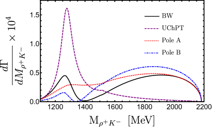
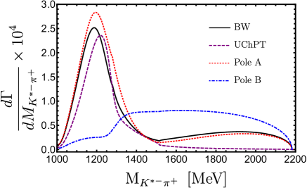
Figure 4: a) $d\Gamma/M_{\rho^{+}K^{-}}$ invariant mass distribution for the $\bar{B}^{0}\to J/\psi\rho^{+}K^{-}$ reaction (black solid line), compared with the curves obtained by considering only: pole $A$ (red dotted line), and pole $B$ (blue dot-dashed line); b) $d\Gamma/M_{K^{*-}\pi^{+}}$ distribution for $\bar{B}^{0}\to J/\psi K^{*-}\pi^{+}$ channel also compared with distributions due to each pole contribution separately. BW is the Breit-Wigner parametrization whereas UChPT stands for Chiral Unitary theory.

In Fig. 4 and 4 we show the $VP$ invariant-mass distributions for $\bar{B}^{0}\to J/\psi\rho^{+}K^{-}$ and $\bar{B}^{0}\to J/\psi K^{*-}\pi^{+}$ reactions, respectively. The dashed lines (labeled UChPT) represent the results obtained using the unitarized amplitudes for the two-body $VP$ final-state interaction [Eq. (17)]. The solid lines (labeled BW) represent the curves obtained if we parametrize the two-body $VP$ amplitudes in Eq. (17) by using a double Breit-Wigner-like shape [Eq. (25)]. In Fig. 4 we also show the individual contributions of both poles A (dotted line) and B (dot-dashed line) in the Breit-Wigner approach.

Note that the phase space for both $\bar{B}^{0}\to J/\psi\rho^{+}K^{-}$ and $\bar{B}^{0}\to J/\psi K^{*-}\pi^{+}$ decays take nonzero values below the corresponding $VP$ threshold as a consequence of the convolution with the vector meson spectral function in order to take into account the finite widths of the $\rho$ and $\bar{K}^{*}$ mesons. This effect is especially relevant for the $\rho\bar{K}$ channel.

On the other hand, the global normalization factor in Eqs. (15) and (16) is the same for both decay channels, and it does not play a relevant role in our results since what matters is the relative strengths and shapes between the mass distribution of the different channels and mechanisms considered. Actually, this global normalization, $C$, is the only free parameter in our model.

It is worth noting that the Chiral Unitary approach used in this case has a range of applicability up to about $1500-1600$ MeV in the invariant mass. We plot the distributions in the whole range, but one should bear in mind that the predictions for the high invariant masses are less reliable.

A first clear observation from Fig. 4 is that the $K_{1}(1270)$ resonant shape dominates the distributions at low invariant masses. However, each distribution is mainly manifesting a different pole associated to the $K_{1}(1270)$. In fact, one would expect from the values of the couplings shown in Table 1 that the pole A would manifest more in the $\bar{K}^{*}\pi$ distribution and the pole B in $\rho\bar{K}$. Indeed, we see in Fig. 4 that the $\rho^{+}K^{-}$ mass distribution has a pronounced peak at $1284$ MeV, which is just the energy region where the highest $K_{1}(1270)$ pole emerges (pole $B$ in Table 1). On the other hand, in Fig. 4 the $K^{*-}\pi^{+}$ distribution peaks at $1185$ MeV, which is the energy region dominated by the lowest $K_{1}$ pole (pole $A$ in Table 1). In addition, the former mass spectrum is narrower than the latter, manifesting the fact that pole B, which couples mostly to $\rho\bar{K}$, is the narrower one, with a width around $146$ MeV. By contrast, the pole $A$, with a width equal to $246$ MeV, is broader than the pole $B$ and couples mostly to $\bar{K}^{*}\pi$, and then causes the peak in the $K^{*-}\pi^{+}$ distribution to be wider.

The previous discussion is also applicable if we look at the BW curves obtained by using the double Breit-Wigner-like amplitudes [Eq. (25)]. The reason of the difference between the UChPT and BW curves is that the unitarization amplitudes in Eq. (17) contain the full $VP$ dynamics and not just the resonant information. We see that this difference is more relevant for the $\rho\bar{K}$ distribution. If we look at the individual contributions of the different poles, we clearly see the dominance of pole $B$ for the $\rho^{+}K^{-}$ case and pole $A$ for the $K^{*-}\pi^{+}$ case.

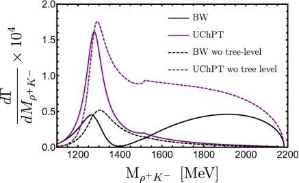
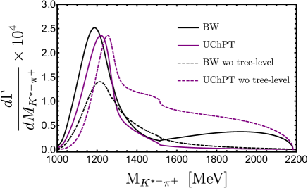
Figure 5: a) $d\Gamma/M_{\rho^{+}K^{-}}$ invariant mass distribution for the $\bar{B}^{0}\to J/\psi\rho^{+}K^{-}$ reaction with and without the tree-level mechanism; b) $d\Gamma/M_{K^{*-}\pi^{+}}$ distribution for the $\bar{B}^{0}\to J/\psi K^{*-}\pi^{+}$ channel also compared with the distribution without interference between tree-level and the resonant part of the amplitude.

Finally, we study the relative importance of the tree-level contribution in Fig. 3 compared to the final-state interaction (implemented here by using the UChPT or the Breit-Wigner approach). This is shown in Fig. 5 where we confront the results obtained considering only the resonant part (dashed lines) with those for the whole mechanism: tree-level plus resonant parts (solid lines). We can see that for the $\bar{K}^{*}\pi$ channel the shapes of the UChPT curves with and without the tree-level contributions are similar in strength but shifted by about 50 MeV. For the double-pole Breit-Wigner parametrization the effect of turning off the tree-level contribution is more visible in the strength of the spectra than in the shift of the curves. It decreases the maximum strength of the peak by half its value. For the $\rho\bar{K}$ channel the UChPT curves exhibit a noticeable difference in their shapes at high energies, but the strength is not altered much in the resonant region.

IV Conclusions

We have theoretically investigated the double-pole structure of the $K_{1}(1270)$ resonance, which was shown in Ref. geng2007 to be dynamically generated through the pseudoscalar-vector meson interaction in coupled channels, by looking at the invariant mass distributions for the $\rho\bar{K}$ and $\bar{K}^{*}\pi$ pairs, respectively, in the $\bar{B}\to J/\psi\rho\bar{K}$ and $\bar{B}\to J/\psi\bar{K}^{*}\pi$ reactions. The final-state interaction mechanism was implemented employing the Chiral Unitary approach, in which the pseudoscalar-vector meson interaction gives rise to the two $K_{1}(1270)$ poles that, in our model, affect both the $\rho\bar{K}$ and $\bar{K}^{*}\pi$ distributions differently. This feature allows us to unveil the double-pole structure in these reactions.

In particular, we have shown that the $\rho\bar{K}$ distribution in the $\bar{B}\to J/\psi\rho\bar{K}$ reaction is dominated by the contribution from the $K_{1}$ highest mass pole, whereas the lowest mass pole contributes more for the $\bar{K}^{*}\pi$ distribution in the $\bar{B}\to J/\psi\bar{K}^{*}\pi$ decay. As we have pointed out, this is due to the values of the coupling constants of those poles to the different channels considered in this work, more specifically, the $\rho\bar{K}$ and $\bar{K}^{*}\pi$ channels. On the other hand, it is important to stress that even though it is possible to see one pole dominance over the other in each distribution, both $VP$ spectra still have the two $K_{1}(1270)$ poles contributing to their shapes. In view of that, we have also modeled the two-body dynamics by using a double-pole Breit-Wigner parametrization such that the contributions of the two poles could be disentangled. In this case, one expects to observe the manifestation of each pole separately in the $VP$ spectra to which they couple most strongly.

An experimental investigation of those reactions would be most welcome to shed light on the nature of $K_{1}(1270)$.

Appendix A $VP$ interaction in the local hidden gauge approach

We evaluate the $VP$ interaction in the local hidden gauge (LHG) approach hidden1 ; hidden2 ; hidden4 ; nagahiro through vector exchange, as depicted in Fig. 6.

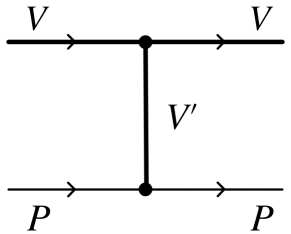
Figure 6: $VP$ interaction through the exchange of vector mesons.

For this we borrow the $VVV$ and $VPP$ Lagrangians from the LHG, given by

$$\mathcal{L}_{VVV}=ig\langle\,(V_{\mu}\partial_{\nu}V^{\mu}-\partial_{\nu}V_{\mu}V^{\mu})V^{\nu}\,\rangle\,,$$ (26)

where $g=M_{V}/2f$ ($M_{V}\approx 800$ MeV, $f=93$ MeV) and

$$\mathcal{L}_{VPP}=-ig\langle V^{\mu}[P,\partial_{\mu}P]\,\rangle\,,$$ (27)

where $\langle\,.\,.\,.\,\rangle$ stands for the trace in $SU(3)$ and $V,\,P$ are the matrices given in Eqs. (4) and (5). The Chiral Lagrangian of Eq. (18) can be obtained from these Lagrangians in the following way. First, we make the approximation that the three-momenta of the vector mesons are very small with respect to the vector meson mass. This is so in our particular case, and hence one takes the limit of negligible three-momenta versus the vector meson mass. In this case, the vector field $V^{\nu}$ in Eq. (26) cannot correspond to an external vector of Fig. 6. This is so because if it were an external vector, then $\nu=1,\,2,\,3$ since $\epsilon^{0}=0$ when $\mathbf{p}_{V}=0$. But then we have $\partial_{\nu}$ which gives rise to a vector three-momentum that is zero. Then, $V^{\nu}$ is the $V^{\prime}$ vector exchanged in Fig. 6 and one has a structure like in the $VPP$ Lagrangian, only with the extra factor $\epsilon_{\mu}\epsilon^{\prime\mu}=-\boldsymbol{\epsilon}^{\prime}\cdot\boldsymbol{\epsilon}$ for the external vectors.

The amplitude for the diagram of Fig. 6 is then given as

$$-it=-g\,(V^{\mu}\partial_{\nu}V_{\mu}-\partial_{\nu}V_{\mu}V^{\mu})_{ij}\,V^{\nu}_{ji}\,\frac{i}{q^{2}-M_{V}^{2}}\,V^{\nu\prime}_{lm}\,[P,\partial_{{\nu}^{\prime}}P]_{ml}$$ (28)

where the indices $i,j,l,m$ are the matrix indices of $P$ and $V$ in Eqs. (4) and (5) written explicitly to obtain the traces.

Since

$$\sum_{pol}\epsilon^{\nu}_{ji}\,\epsilon^{{\nu}^{\prime}}_{lm}=\Big{(}-g^{\nu{\nu}^{\prime}}+\frac{q^{\nu}q^{{\nu}^{\prime}}}{M^{2}_{V}}\Big{)}\,\delta_{jl}\,\delta_{im}\,,$$ (29)

we readily obtain, neglecting the term $q^{\nu}q^{{\nu}^{\prime}}/M^{2}_{V}$ consistently with the approximations done,

$$-it=-i\frac{g^{2}}{M^{2}_{V}}\langle\,(V^{\mu}\partial_{\nu}V_{\mu}-\partial_{\nu}V_{\mu}V^{\mu})\,[\,P,\partial^{\nu}P\,]\,\,\rangle\,,$$ (30)

and hence

$$\mathcal{L}=-\frac{1}{4f^{2}}\,\langle\,\,[\,V^{\mu},\partial_{\nu}V^{\mu}]\,[P,\partial^{\nu}P]\,\rangle\,,$$ (31)

which is the Chiral Lagrangian of Ref. Birse , as shown in Eq. (18). This equivalence was already shown in a particular case for the $\rho\pi$ interaction in nagahiro . Here we have made a general derivation.

As shown in Ref. Roca:2005nm , the $s$-wave projected potential for transition of channel $i$ to $j$ is given by

$$V_{ij}=C_{ij}\,\frac{\boldsymbol{\epsilon}\cdot\boldsymbol{\epsilon^{\prime}}}{8f^{2}}\,\Big{(}3s-(M^{2}+m^{2}+M^{\prime\,2}+m^{\prime\,2})-\frac{1}{s}(M^{2}-m^{2})(M^{\prime\,2}-m^{\prime\,2})\Big{)}\,,$$ (32)

where $M$, $m$, $M^{\prime}$, $m^{\prime}$ are the initial and final vector and pseudoscalar masses, respectively, $\boldsymbol{\epsilon}$ and $\boldsymbol{\epsilon^{\prime}}$ the polarization vectors of the initial and final vectors, and $C_{ij}$ are coefficients given in Table II of Ref. Roca:2005nm . Of relevance here are the coefficients $C_{\rho K,\rho K}=C_{K^{*}\pi,K^{*}\pi}=-2$; $C_{\rho K,K^{*}\pi}=1/2$.

Appendix B Pseudoscalar exchange in the vector pseudoscalar interaction

In misha it was pointed out that a source of the $VP$ interaction is given by the diagram in Fig. 7.

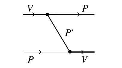
Figure 7: Source for $VP$ interaction through the exchange of pseudoscalars.

This interaction was also considered in nakamura in the study of the $VP$ interaction in the $D^{+}\to K^{-}\pi^{+}\pi^{+}$ reaction; however, this was done in addition to the vector exchange discussed here in Appendix A, and it was found that the vector exchange is far more important than the contribution of pseudoscalar exchange nakamura ; nakamurapriv . We address this issue here in connection with our $VP$ channels $\rho\bar{K}$, $\bar{K}^{*}\pi$ that we have in the problem under study.

The effect of pseudoscalar exchange was already addressed in the study of the vector-vector interaction in raquel ; gengvec . The box diagram of Fig. 8

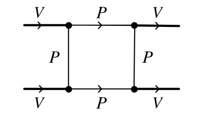
Figure 8: Box diagram in the $VV$ interaction given by $P$ exchange and intermediate $PP$ states.

was evaluated exactly with the full structure of the four intermediate propagators. Then the $VV\to VV$ potential obtained there was added to the one obtained from $VV\to VV$ with a single vector exchanged discussed in Appendix A and the whole potential was iterated with the Bethe-Salpeter equation. It was found that the real part of the box diagrams was negligible compared to the vector exchange, but the imaginary part provided a source of decay for the found $VV$ molecular bound states. This was relevant because the bound $VV$ states without this term had no width except for a small one when considering the width of the vector mesons. However, the $PP$ intermediate states have a small mass and provide a large phase space for the decay. The box gave rise to a width of the $VV$ states but no change in their mass.

The equivalent diagram to Fig. 8 for the $VP$ interaction, based on Fig. 7, is given in Fig. 9.

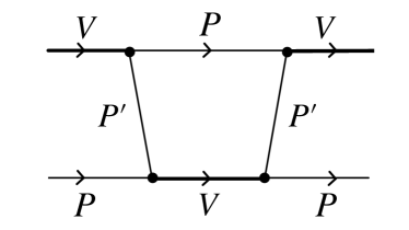
Figure 9: Box diagram contributing to $VP\to VP$.

We evaluate its contribution here for the case of our interest $\rho\bar{K}\to\rho\bar{K}$ and the term is depicted in Fig. 10.

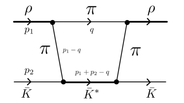
Figure 10: Box diagram for $\rho\bar{K}\to\rho\bar{K}$ through a $\bar{K}^{*}\pi$ intermediate state.

However, unlike in the case of $VV$, where we need two steps in the $VV\to PP\,\times\,PP\to VV$ to obtain a $VV\to VV$ interaction term, here a single step $VP\to PV$ driven by pseudoscalar exchange already provides a $VP\to PV$ interaction term. In order to quantify the relevance of the pseudoscalar exchange versus vector exchange, we compare the contributions of Fig. 11 with Fig. 11 and Fig. 12 with Fig. 12.

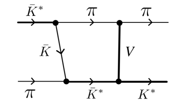
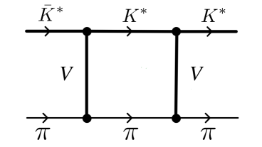
Figure 11: Two steps one meson exchange: a) Pseudoscalar and vector exchange; b) Vector and vector exchange.

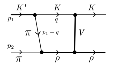
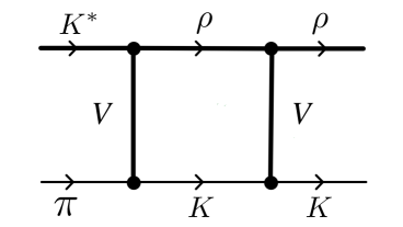
Figure 12: Same as Fig. 11 for the $K^{*}\pi\to K\rho$ transition.

We find it sufficient to evaluate the diagrams close to the $\rho K$ threshold to benefit from the approximations discussed in Appendix A when the three-momenta of the vectors compared to their masses are negligible. In this case, we have $\epsilon^{0}=0$ for the $\rho$ and given the fact that the large contribution from the diagram involving intermediate $K^{*}\pi$ comes when $\bar{K}^{*}\pi$ is close to on shell and the $\bar{K}^{*}$ has a small momentum, we also take $\epsilon^{0}=0$ for the $\bar{K}^{*}$. In the Appendix of Ref. ramosakai it was found that this assumption gave surprisingly good results up to relatively large momenta of the $\bar{K}^{*}$ compared to a full relativistic calculation for timelike $\bar{K}^{*}$.

To evaluate the pseudoscalar exchange potential we need the Lagrangian of Eq. (27) and the isospin structure of the $|\,\rho\bar{K},I=1/2,I_{3}=1/2\,\rangle$ and $|\,\bar{K}^{*}\pi,I=1/2,I_{3}=1/2\,\rangle$ states given by

$$|\,\rho\bar{K},I=1/2,I_{3}=1/2\,\rangle = \sqrt{\frac{2}{3}}|\rho^{+}K^{-}\rangle-\frac{1}{\sqrt{3}}|\rho^{0}\bar{K}^{0}\rangle$$

$$|\,\bar{K}^{*}\pi,I=1/2,I_{3}=1/2\,\rangle = -\Big{(}\sqrt{\frac{2}{3}}|\pi^{+}K^{*-}\rangle-\frac{1}{\sqrt{3}}|\pi^{0}\bar{K}^{{}^{*}0}\rangle\Big{)}\,.$$ (33)

For the vector exchange potentials we use Eq. (32).

The contribution of the loop diagram of Fig. 11 is given by

$$-it_{11a} = \int\,\frac{d^{4}q}{(2\pi)^{4}}\,g^{2}\,(\boldsymbol{\epsilon}_{K^{*}}\cdot\boldsymbol{q})\,(\boldsymbol{\epsilon^{\prime}}_{K^{*}}\cdot\boldsymbol{q})\,\frac{i}{q^{2}-m^{2}_{\pi}+i\epsilon}\,\frac{i}{(p_{1}-q)^{2}-m^{2}_{K}+i\epsilon}\times$$ (34)

$$\times \frac{i}{(p_{1}+p_{2}-q)^{2}-m^{2}_{K^{*}}+i\epsilon}\,(-i\tilde{V}_{K^{*}\pi,K^{*}\pi})\,(\boldsymbol{\epsilon^{\prime}}_{K^{*}}\cdot\boldsymbol{\epsilon^{\prime\prime}}_{K^{*}})\,,$$

with $\tilde{V}_{ij}$ given by Eq. (32) removing the $\boldsymbol{\epsilon}\cdot\boldsymbol{\epsilon}^{\prime}$ factor. The $q^{0}$ integration is performed analytically using contour integration. For this purpose, we use

$$\frac{1}{q^{2}-m^{2}_{\pi}}=\frac{1}{2\omega(q)}\,\Big{(}\frac{1}{q^{0}-\omega(q)+i\epsilon}-\frac{1}{q^{0}+\omega(q)-i\epsilon}\Big{)}\,,$$ (35)

and the same for the $\bar{K}$ propagator. For the $K^{*}$ propagator, because the heavy $K^{*}$ mass and the fact that it propagates in the $s$ channel, where it is close to on shell, or eventually on shell, it is sufficient to take into account only the first term in Eq. (35) $-$ the positive-energy part of the propagator.

We further take into account that $\sum_{pol}\epsilon^{\prime}_{\bar{K}^{*}\,i}\,\epsilon^{\prime}_{\bar{K}^{*}\,j}=\delta_{ij}$ and that $\int\,d^{3}q\,\mathbf{q}_{i}\,\mathbf{q}_{j}\,f(\mathbf{q}^{2})=\delta_{ij}\,\int\,d^{3}q\,\mathbf{q}^{2}\,f(\mathbf{q}^{2})/3$, which projects into $s$ wave the operator $q_{i}\,q_{j}$, and we find

$$t_{11a} = -\frac{1}{3}\,g^{2}\,(\boldsymbol{\epsilon}_{K^{*}}\cdot\boldsymbol{\epsilon}^{\prime\prime}_{K^{*}})\,\tilde{V}_{K^{*}\pi,K^{*}\pi}\,\int\,\frac{d^{3}q}{(2\pi)^{3}}\,\boldsymbol{q}^{2}\,\frac{1}{8\,\omega_{\pi}\,\omega_{K}\,\omega_{K^{*}}}\,\Big{\{}\frac{1}{\sqrt{s}-\omega_{\pi}-\omega_{K^{*}}+i\frac{\Gamma_{K^{*}}}{2}}\times$$ (36)

$$\times \Big{(}\frac{1}{p^{0}_{1}-\omega_{\pi}-\omega_{K}+i\epsilon}+\frac{1}{p^{0}_{2}-\omega_{K}-\omega_{K^{*}}+i\frac{\Gamma_{K^{*}}}{2}}\Big{)}-\frac{1}{p^{0}_{1}+\omega_{K}+\omega_{\pi}}\times$$

$$\times \frac{1}{p^{0}_{2}-\omega_{K}-\omega_{K^{*}}+i\frac{\Gamma_{K^{*}}}{2}}\Big{\}}\Big{(}\frac{\Lambda^{2}-m^{2}_{\pi}}{\Lambda^{2}+\boldsymbol{q}^{2}}\Big{)}^{2}\,,$$

where $\omega_{i}=\sqrt{m^{2}_{i}+\boldsymbol{q}^{2}}$, we include the $K^{*}$ width, and we have added a form factor for the pseudoscalar exchange. We have taken $\Lambda=1200$ MeV, was used in Ref. raquel , and in addition we cut the $\boldsymbol{q}$ integration to $\boldsymbol{q}_{max}=900$ MeV, an inherent cutoff in the loop integration associated with the use of the chiral potentials in Ref. Roca:2005nm .

Using the same argumentation, we obtain for the diagram of Fig. 12

$$t_{12a} = \frac{4}{3}\,g^{2}\,\frac{1}{3}\,(\boldsymbol{\epsilon}_{K^{*}}\cdot\boldsymbol{\epsilon}_{\rho})\,\tilde{V}_{\rho K,\rho K}\,\int\,\frac{d^{3}q}{(2\pi)^{3}}\,\boldsymbol{q}^{2}\,\frac{1}{8\,\omega_{\pi}\,\omega_{K}\,\omega_{\rho}}\,\Big{\{}\frac{1}{\sqrt{s}-\omega_{K}-\omega_{\rho}+i\frac{\Gamma_{\rho}}{2}}\times$$ (37)

$$\times \Big{(}\,\frac{1}{p^{0}_{1}-\omega_{\pi}-\omega_{K}+i\epsilon}+\frac{1}{p^{0}_{2}-\omega_{\pi}-\omega_{\rho}+i\frac{\Gamma_{\rho}}{2}}\,\Big{)}-\frac{1}{p^{0}_{1}+\omega_{\pi}+\omega_{K}}\times$$

$$\times \frac{1}{p^{0}_{2}-\omega_{\pi}-\omega_{\rho}+i\frac{\Gamma_{\rho}}{2}}\Big{\}}\Big{(}\frac{\Lambda^{2}-m^{2}_{\pi}}{\Lambda^{2}+\boldsymbol{q}^{2}}\Big{)}^{2}\,.$$

The diagrams of Figs. 11 and 12 are easily evaluated and we obtain

$$t_{11b} = (\boldsymbol{\epsilon}_{K^{*}}\cdot\boldsymbol{\epsilon}^{\prime\prime}_{K^{*}})\,\int\,\frac{d^{3}q}{(2\pi)^{3}}\,\frac{1}{2\,\omega_{\pi}}\,\frac{1}{2\,\omega_{K^{*}}}\,\frac{1}{\sqrt{s}-\omega_{\pi}-\omega_{K^{*}}+i\frac{\Gamma_{K}^{*}}{2}}\,(\tilde{V}_{K^{*}\pi,K^{*}\pi})^{2}\,,$$ (38)

$$t_{12b} = (\boldsymbol{\epsilon}_{K^{*}}\cdot\boldsymbol{\epsilon}_{\rho})\,\int\,\frac{d^{3}q}{(2\pi)^{3}}\,\frac{1}{2\,\omega_{K}}\,\frac{1}{2\,\omega_{\rho}}\,\frac{1}{\sqrt{s}-\omega_{K}-\omega_{\rho}+i\frac{\Gamma_{\rho}}{2}}\,(\tilde{V}_{K^{*}\pi,\rho K}\,\tilde{V}_{\rho K,\rho K})\,.$$ (39)

Next we evaluate the diagram of Fig. 10 which contains two pseudoscalar exchanges. Then, we find for the product of the two left vertices of Fig. 10,

$$-i\tilde{t}_{\rho\bar{K}\to\bar{K}^{*}\pi}=4g^{2}\,(\mathbf{q}\cdot\boldsymbol{\epsilon}_{\rho})\,(\mathbf{q}\cdot\boldsymbol{\epsilon}_{\bar{K}^{*}})\,,$$ (40)

and for the loop of Fig. 10 including the propagators we find

$$-it_{\textrm{10}} = 16g^{4}\,\int\frac{d^{4}q}{(2\pi)^{4}}(\mathbf{q}\cdot\boldsymbol{\epsilon}_{\rho})\,(\mathbf{q}\cdot\boldsymbol{\epsilon}_{\bar{K}^{*}})\,(\mathbf{q}\cdot\boldsymbol{\epsilon}_{\bar{K}^{*}})\,(\mathbf{q}\cdot\boldsymbol{\epsilon}^{\prime}_{\rho})\,\Big{[}\frac{i}{(p_{1}-q)^{2}-m^{2}_{\pi}+i\epsilon}\Big{]}^{2}\times$$ (41)

$$\times \frac{i}{q^{2}-m^{2}_{\pi}+i\epsilon}\,\frac{i}{(p_{1}+p_{2}-q)^{2}-m^{2}_{\bar{K}^{*}}+i\epsilon}\,,$$

which, upon sum over the $\bar{K}^{*}$ polarizations, $\sum_{pol}\epsilon^{i}_{\bar{K}^{*}}\,\epsilon^{j}_{\bar{K}^{*}}=\delta^{ij}$, can be written as

$$-it_{10} = -i\,16\,g^{4}\,\frac{\partial}{\partial m_{\pi}^{\prime\,2}}\,\Big{\{}i\,\int\frac{d^{4}q}{(2\pi)^{4}}\,|\mathbf{q}|^{2}\,(\mathbf{q}\cdot\boldsymbol{\epsilon}_{\rho})\,(\mathbf{q}\cdot\boldsymbol{\epsilon}^{\prime}_{\rho})\,\frac{1}{(p_{1}-q)^{2}-m_{\pi}^{\prime\,2}+i\epsilon}\,$$ (42)

$$\times \frac{1}{q^{2}-m^{2}_{\pi}+i\epsilon}\,\frac{1}{(p_{1}+p_{2}-q)^{2}-m^{2}_{\bar{K}^{*}}+i\epsilon}\,\Big{\}}\Big{|}_{m_{\pi}^{\prime}=m_{\pi}}\,.$$

The use of the partial derivative with respect to $m_{\pi}^{\prime\,2}$ saves us one propagator, and then by decomposing the propagators as in Eq. (35) and keeping only the positive-energy part for the heavy $\bar{K}^{*}$, we can immediately perform the $q^{0}$ integration analytically using Cauchy’s residues, with the result

$$t_{10} = \frac{16}{3}\,g^{4}\,(\boldsymbol{\epsilon}_{\rho}\cdot\boldsymbol{\epsilon}^{\,\,\prime}_{\rho})\,\frac{{\partial}}{\partial m^{\prime\,2}_{\pi}}\,\int\,\frac{dq\,q^{6}}{2\pi^{2}}\,\frac{1}{2\omega}\,\frac{1}{2\omega^{\prime}}\,\frac{1}{2\omega^{*}}\,\Big{(}\frac{\Lambda^{2}-m^{2}_{\pi}}{\Lambda^{2}+\mathbf{q}^{2}}\Big{)}^{4}\,\Big{\{}\frac{1}{\sqrt{s}-\omega-\omega^{*}\,+\frac{i\Gamma^{*}}{2}}\times\,$$

$$\times \Big{(}\frac{1}{p^{0}_{1}-\omega-\omega^{\prime}+i\epsilon}\,+\frac{1}{p^{0}_{2}-\omega^{\prime}-\omega^{*}+\frac{i\Gamma^{*}}{2}}\Big{)}\,-\frac{1}{p^{0}_{1}+\omega+\omega^{\prime}}\,\frac{1}{p^{0}_{2}-\omega^{\prime}-\omega^{*}+\frac{i\Gamma^{*}}{2}}\Big{\}}\,,$$

where $\omega=\sqrt{m^{2}_{\pi}+\mathbf{q}^{2}}$, $\omega^{\prime}=\sqrt{m^{\prime 2}_{\pi}+\mathbf{q}^{2}}$, $\omega^{*}=\sqrt{m^{2}_{\bar{K}^{*}}+\mathbf{q}^{2}}$, $\Gamma^{*}$ is the $\bar{K}^{*}$ width, and the energy of $VP$ in the rest frame $\sqrt{s}=p^{0}_{1}+p^{0}_{2}$.

The magnitude of $t_{10}$ should be compared to the term coming from vector exchange $t_{vex}$, which is evaluated following Appendix A and gives

$$t_{vex}=-2\,\frac{1}{4f^{2}}\,(p_{1}+p_{3})(p_{2}+p_{4})\,(\boldsymbol{\epsilon}_{\rho}\cdot\boldsymbol{\epsilon}^{\prime}_{\rho})\,,$$ (44)

which can be cast as in Eq. (32) projected in $s$ wave. We find at the $\rho\bar{K}$ threshold

$$t_{vex} = 87.78\,;$$

$$t_{10} = 0.25-i\,4.10\,.$$ (45)

We summarize the results obtained in Table 2 for the energy $\sqrt{s}=1270$ MeV, which is the nominal energy of the $K_{1}(1270)$. As discussed above, we take the external three-momenta to be zero and the on-shell energies $p^{0}_{1}$, $p^{0}_{2}$ to be $\sqrt{s}=1270$ MeV. For $t_{10}$ we use the $\rho K$ threshold dynamics, which leads to Eq. (45).

Table 2: Values of the different box diagrams calculated at $\sqrt{s}=1270$ MeV. The different $t_{i}$ refer to the corresponding diagram of Fig. i.

	$\tilde{V}_{\bar{K}^{*}\pi,\bar{K}^{*}\pi}$	$\tilde{V}_{\rho K,\rho K}$	$\tilde{V}_{\bar{K}^{*}\pi,\rho K}$
	$-82.25$	$-89.34$	$21.85$
$t_{11a}$	$t_{11b}$	$t_{12a}$	$t_{12b}$	$t_{10}$
$-0.80-i1.87$	$-64.7-i61.1$	$-1.96-i3.01$	$18.73+i6.73$	$0.25-i4.10$

As we can see, the contribution of the $t_{11a}$, with $K$ exchange, is very small compared to the tree-level $V_{\bar{K}^{*}\pi,\bar{K}^{*}\pi}$, or to the box diagram of Fig. 11 $-$ about $1\%$ for the real part or $3\%$ for the imaginary compared to $t_{11b}$ $-$ which gives an idea of the relative weight of the pseudoscalar exchange. One should note that we also have a diagram in which the vector exchange appears to the left and the pseudoscalar exchange appears to the right in Fig. 11, which would double its contribution but, although smaller than the contribution of Fig.  11, we also have an extra contribution of the type of $t_{11b}$ coming from Fig. 11 with $\rho K$ intermediate state, so the corrections from pseudoscalar exchange are really small. If we look at $t_{12a}$ and $t_{12b}$ the effect seems to be relatively larger: $10\%$ for the real part and $44\%$ for the imaginary part. But, if one compares the imaginary part with the real part is only $16\%$ correction. Once again, we would double the strength of this mechanism by exchanging the $\pi$ and $V$ exchange in Fig. 12, but we also double the strength of Fig. 12 by adding $K^{*}\pi$ in the intermediate state. We should also note that the relatively larger corrections found in the case of the $\bar{K}^{*}\pi\to\rho\bar{K}$ transition in Fig. 12 affect an amplitude which, as seen in Appendix A, has a strength $1/4$ of the diagonal $\bar{K}^{*}\pi\to\bar{K}^{*}\pi$, $\rho\bar{K}\to\rho\bar{K}$ transitions, as a consequence of which there is a small mixing of $K^{*}\pi$ and $\rho K$ which is not affected by the maximum $16\%$ correction to the $K^{*}\pi\to\rho K$ transition term that has a strength of $1/4$ of the diagonal ones.

The contribution of the box diagram of Fig. 10 with the exchange of two pions given by the $t_{10}$ in Table 2 is also very small, and so is that of the similar box diagram for $K^{*}\pi\to K^{*}\pi$ with $\rho\bar{K}$ intermediate state.

References

- (1) G. W. Brandenburg, et al. Phys. Rev. Lett. 36, 703 (1976)
- (2) C. Daum et al. [ACCMOR], Nucl. Phys. B 187, 1-41 (1981)
- (3) P. A. Zyla et al. [Particle Data Group], PTEP 2020 8, 083C01 (2020)
- (4) M. Suzuki, Phys. Rev. D 47, 1252-1255 (1993)
- (5) A. Tayduganov, E. Kou and A. Le Yaouanc, Phys. Rev. D 85, 074011 (2012)
- (6) Z. Q. Zhang, H. Guo and S. Y. Wang, Eur. Phys. J. C 78, 219 (2018)
- (7) L. Roca, E. Oset and J. Singh, Phys. Rev. D 72, 014002 (2005)
- (8) U.-G. Meißner, Symmetry 12, no.6, 981 (2020).
- (9) G. Y. Wang, L. Roca and E. Oset, Phys. Rev. D 100, 074018 (2019)
- (10) G. Y. Wang, L. Roca, E. Wang, W. H. Liang and E. Oset, Eur. Phys. J. C 80, 388 (2020)
- (11) Y. Zhang, E. Wang, D. M. Li and Y. X. Li, Chin. Phys. C 44, 093107 (2020).
- (12) L. Micu, Nucl. Phys. B 10, 521-526 (1969).
- (13) A. L. Yaouanc, L. Oliver, O. Pene, J. C. Raynal, Phys. Rev. D 8, 2223-2234 (1973).
- (14) E. Santopinto, R. Bijker, Pys. Rev. C 82, 062202 (2010).
- (15) A. Bramon, A. Grau, and G. Pancheri, Phys. Lett. B 283, 416 (1992).
- (16) L. S. Geng, E. Oset, L. Roca and J. A. Oller, Phys. Rev. D 75, 014017 (2007)
- (17) J. A. Oller, E. Oset, and J. R. Pelaez, Phys. Rev. Lett. 80, 3452 (1998).
- (18) J. A. Oller, E. Oset, and A. Ramos, Prog. Part. Nucl. Phys. 45, 157 (2000).
- (19) J. A. Oller, E. Oset, and J. R. Pelaez, Phys. Rev. D 59, 074001 (1999); Phy. Rev. D 60, 099906 (1999) (Erratum); Phy. Rev. D 75, 099903 (2007).
- (20) M. C. Birse, Z. Phys. A 355, 231-246 (1996).
- (21) M. Bando, T. Kugo and K. Yamawaki, Phys. Rept. 164, 217-314 (1988).
- (22) M. Harada and K. Yamawaki, Phys. Rept. 381, 1-233 (2003).
- (23) U. G. Meissner, Phys. Rept. 161, 213 (1988).
- (24) H. Nagahiro, L. Roca, A. Hosaka and E. Oset, Phys. Rev. D 79, 014015 (2009).
- (25) J. P. Dedonder, R. Kaminski, L. Lesniak and B. Loiseau, Phys. Rev. D 89, 094018 (2014).
- (26) F. Niecknig and B. Kubis, JHEP 10, 142 (2015) doi:10.1007/JHEP10(2015)142 [arXiv:1509.03188 [hep-ph]].
- (27) S. X. Nakamura, Phys. Rev. D 93, 014005 (2016).
- (28) L. L. Chau, Phys. Rept. 95, 1-94 (1983).
- (29) R. Molina and E. Oset, Phys. Rev. D 80, 114013 (2009).
- (30) M. Mai, B. Hu, M. Doring, A. Pilloni and A. Szczepaniak, Eur. Phys. J. A 53, 177 (2017).
- (31) R. Molina, D. Nicmorus and E. Oset, Phys. Rev. D 78, 114018 (2008).
- (32) L. S. Geng and E. Oset, Phys. Rev. D 79, 074009 (2009).
- (33) S. X. Nakamura, private communication.
- (34) S. Sakai, E. Oset and A. Ramos, Eur. Phys. J. A 54, 10 (2018).