Extremely Correlated Superconductors

Abstract

Superconductivity in the  $t$-$J$  model is studied by extending the recently introduced extremely correlated fermi liquid theory. Exact equations for the Greens functions are obtained by generalizing Gor’kov’s equations to include extremely strong local repulsion between electrons of opposite spin. These equation are expanded in a parameter $\lambda$ representing the fraction of double occupancy, and the lowest order equations are further simplified near $T_{c}$, resulting in an approximate integral equation for the superconducting gap. The condition for $T_{c}$ is studied using a model spectral function embodying a reduced quasiparticle weight $Z$ near half-filling, yielding an approximate analytical formula for $T_{c}$. This formula is evaluated using parameters representative of single layer High-$T_{c}$ systems. In a narrow range of electron densities that is necessarily separated from the Mott-Hubbard insulator at half filling, we find a typical $T_{c}$$\sim$$10^{2}$K.

Keywords The tJ Model, cuprates d-wave superconductivity, correlated Gor‘kov equation

1 Introduction

The single band  $t$-$J$  model Eq. (1),[1, 2], and the closely related strong coupling Hubbard model have attracted much attention in recent years. In large part the interest is due to the potential relevance of these models in describing the phenomenon of High $T_{c}$ superconductivity, discovered in cuprate materials in 1987 [3] and later, in other materials. These models lead to a single sheet of the fermi surface, and are specified by fixing the band hopping $t$ and the exchange energy $J$ for the  $t$-$J$  model, or equivalently $4t^{2}/U$ for the strong coupling ($U\gg t$) Hubbard model, where the interaction is given by $V_{Hub.}=U\sum_{i}n_{i\downarrow}n_{i\uparrow}$. The exotic possibility of superconductivity arising from such inherently repulsive systems, is surprising from a theoretical perspective, and also challenging. Significant theoretical work using a variety of tools on the strong coupling Hubbard model and the extremely strong coupling  $t$-$J$  models [4, 5, 6, 7, 8, 9, 11, 10, 12, 13, 14, 15, 16] has given useful insights into the role of strong correlations in cuprate superconductivity. However given the non-triviality of the theoretical task of analytically solving these models, progress in that direction has been slow.

In this work we extend the extremely correlated fermi liquid theory (ECFL) [17, 18] recently formulated to overcome the analytical difficulties of the strong coupling models, to include superconducting type broken symmetry. Upon cooling the normal metallic state, a superconducting instability is expected to arise, and our main goal in this study is to determine the conditions for the occurrence of this state, and to provide its detailed description.

In order to motivate these calculations of the superconducting state, it is useful to summarize the main features of ECFL theory as applied to the normal (non-superconducting) state so far. We provide a broad overview next, further details can be found in Ref. ([17, 18]).

The methodology developed in this theory starts with exact functional differential equations for the various Greens function, obtained using the Tomonaga-Schwinger approach of external potentials. These equations incorporate the modification of the anti-commutation relations between the fermion operators due to Gutzwiller projection (see Eq. (5)). While providing a formally exact starting point for us, these equations are not yet amenable to systematic approximations. The core difficulty is that an additional set of terms arise from this modified non-canonical anticommutator structure Eq. (5). These non-canonical terms multiply the most singular term in the equation, namely the Dirac delta function (originating in the time derivative of the time ordering $\Theta$ functions in the Greens functions). For an explicit example, note the $\gamma$ term multiplying the delta function in Eq. (34).

In order to make progress, we therefore need to go beyond the established framework of Tomonaga-Schwinger. The first development in ECFL is that the above inconvenient feature of a non-canonical coefficient of the delta function, is eliminated by factoring the Greens function into two parts, the auxiliary Greens function ${\bf g}$ and the caparison function $\widetilde{\mu}$ (see Eq. (46) and the discussion in the text following it). The auxiliary Greens function ${\bf g}$ now satisfies a canonical equation (as in Eq. (51) by ignoring the term involving ${\bm{f}}$), while the caparison function $\widetilde{\mu}$ accounts for the non-canonical nature of the original equation (as in Eq. (52)). This factorization process and the resulting equations are exact.

As the next development, we introduce a parameter $\lambda$ in the range $0\leq\lambda\leq 1$ into these exact equations. Setting $\lambda$$=$$0$ gives the uncorrelated system, while $\lambda$$=$$1$ gives the exact equations of the strongly correlated system. The $\lambda$ parameter has a formal similarity to the expansion parameter $\frac{1}{2S}$ used in the Dyson-Maleev (or Holstein-Primakoff) formulations [19, 20] of the spin-wave theory of magnets. The magnetic models involve spin operators satisfying the SU(2) (angular momentum) Lie algebra. They can be approached using different strategies. On the one hand we may think of spins as canonical bosons with a constraint on their occupation number $n^{b}_{i}$ at any site $i$, namely $n^{b}_{i}=0,1,\ldots 2S$. This constraint can be implemented using a repulsive interaction between bosons $Un^{b}_{i}(n^{b}_{i}-1)\ldots(n^{b}_{i}-2S)$, and finally letting $U$$\to$$\infty$. This bosonic Hubbard model is difficult to solve, since the large energy scale $U$ makes the use of perturbation theory impractical. On the other hand we can employ the Dyson-Maleev (or Holstein-Primakoff) non-linear mappings to bosons, and expand the relevant Heisenberg equations of motion in a series in $\frac{1}{2S}$. This gives an efficient way of solving the models to considerable precision at fairly low orders in $\frac{1}{2S}$. This latter method is parallel to the $\lambda$ expansion employed here, since the modified anticommutators Eq. (5) also yield a (non-canonical) Lie algebra.This analogy is discussed further in Ref. ([18]) (Sec. 6). In a different setting, the parameter $\lambda$ can also be related to the fraction of doubly occupied states [21] (see Appendix. A).

The parameter $\lambda$ serves two important and related objectives. Firstly it provides a continuous path between the uncorrelated and the fully correlated system equations. Since $0\leq\lambda\leq 1$, dialing it up from $0$ does not involve invoking a large energy scale, unlike for example, dialing up $U$ in the Hubbard model. This (isothermal) continuity enables the ECFL method to retain the ideal (i.e. non-interacting) fermi surface volume at low T. This ideal volume is expected for weakly interacting fermi systems from the Luttinger-Ward perturbative arguments [22], and importantly, survives the transition to extremely strongly correlated regions, as argued recently using non-perturbative arguments [23]. Lastly, the ideal volume is also seen in photoemission studies of overdoped and optimally doped cuprate superconductors in the normal state [24], which provide a useful starting point for our study.

The second aspect of $\lambda$ is that it can be used to organize a systematic power series expansion, analogous in spirit to the skeleton graph expansion of Dyson [25] in perturbative theories. This $\lambda$ expansion can be carried out order by order, leading to a set of successive equations that are amenable to numerical study. A question might arise, whether a low order calculation in this expansion can capture the strongly correlated limit. For answering this, it is useful to examine the results for the $d=\infty$ Hubbard model at $U=\infty$, where numerically exact results are available from the dynamical mean field theory [26]. The $\lambda$ expansion to ${\cal O}(\lambda^{2})$ is compared with the exact numerical result from the dynamical mean field theory [27], in Fig. (6) of Ref. ([28]). This shows that the calculated quasiparticle weight $Z$ vanishes upon approaching a density of $1$-particle per site, i.e. half filling. This vanishing is a hallmark of the strong correlation limit, where the Mott-Hubbard insulating state is realized. In the above $d=\infty$ study, and also in the case of the 2-dimensional  $t$-$J$  model [29, 30, 31], the $\lambda$ expansion describes an extremely correlated Fermi liquid state, characterized by a small quasiparticle weight that vanishes near the Mott-Hubbard insulator, accompanied by a rich set of low energy scales located above the (strongly suppressed) effective fermi temperature. The ${\cal O}({\lambda}^{2})$ equations for the normal state have been applied to calculations of the asymmetric photoemission lines[32, 30, 31], and most recently the calculation of the almost T-linear resistivity in single layer cuprates[29].

In this paper we extend the above formalism to the case where superconducting order emerges at low temperatures. This requires a non-trivial generalization to the superconducting state of the various steps of the ECFL theory highlighted above. In a similar fashion to the normal state, we first obtain exact equations for the normal and anomalous Greens functions for the  $t$-$J$  model. These equations generalize Gor’kov’s equations for BCS type weak coupling superconductivity[33] by including the effect of extremely strong local repulsion between electrons. These equations are studied further using a specific decomposition of the Greens functions into two pieces (see Eq. (46)). This step is followed by a systematic expansion in a parameter $\lambda$. This leads to an set of equations Eq. (51, 52, 54), iterating these in $\lambda$ to all orders constitutes the exact answer. In the present work, we perform a leading order calculation.

In order to obtain explicit results, Eq. (51, 52, 54) are further simplified near $T_{c}$ where the order parameter is small, leading to simplified versions of these in Eq. (55, 56, 57). These are treated to ${\cal O}({\lambda}^{2})$, and the lowest order condition for $T_{c}$ is formulated in Eq. (68). In summary Eq. (68) is the leading order term near $T_{c}$, within the $\lambda$ expansion, and constitutes an important formal result of the present work. In principle it should be possible to find further systematic equations to higher order, and also to extend the results for $T\ll T_{c}$ following the procedure laid out here. In this work we are content to study this first set in detail. The transition temperature is given from Eq. (68), which is expressed in terms of the electronic Greens function, renormalized by strong correlations. In this renormalization the short ranged Hubbard-Gutzwiller terms are dominant, and the pairing energy causing the instability, is provided by the much smaller exchange energy $J$. This equation exhibits both a tendency towards an insulating state due to a diminished quasiparticle weight, and a tendency towards superconductivity due to the exchange term $J$. Their competing tendencies play out in Eq. (68) and the closely related Eq. (70). These equations determine whether superconductivity is found at all, and further identifies the model parameters that promote it. When the superconducting state is found, they also provides an estimate of the range of densities and temperatures which favor it.

The conditions Eq. (68, 70) are evaluated using a simple phenomenological electronic spectral function, modeling strong correlations near half filling in terms of a density dependent quasiparticle weight $Z$ and a wide background. This model has the advantage of leading to an explicit analytical formula for $T_{c}$, in terms of the various parameters of the  $t$-$J$  model, thus allowing for a thorough understanding of the role of different parameters on the result. Evaluating this expression we find that the model supports a d-wave superconducting phase consistent with data [36, 37], located away from half filling. The $T_{c}$ is found to be typically $\sim$$10^{2}$K, i.e. an order of magnitude smaller than that of the model Eq. (2) where the sole difference from the  $t$-$J$  model is that short ranged Hubbard-Gutzwiller type correlations are ignored, in a range of densities determined by the band parameters. The temperature-density phase diagram has the form of a tapered tower Fig. (1). A smooth dome structure reported in cuprates, is replaced here by a somewhat narrow density range and an exaggerated height near the peak. The location of the peak can be varied by choosing the hopping parameters, but always remains well-separated from the insulating limit.

The paper is organized as follows. In Section (2) we define the  $t$-$J$  Hamiltonian, express it in terms of the correlated fermionic operators, and outline the method of external potentials employed to generate the exact dynamical equations for the electron Greens function ${\cal G}$ and the Gor’kov anomalous Greens function ${\cal F}$. In Section (3) the equation is expanded in $\lambda$ and further simplified near $T_{c}$. In Section (4) the condition for $T_{c}$ is evaluated using a model spectral function. This section contains expressions that involve only the electronic spectral function, and might be directly accessible to readers who are more interested in the concrete results. In Section (5) we conclude with a discussion of the results.

2 Theoretical Preliminaries

The  $t$-$J$  Hamiltonian [1, 2] is

$$H_{\mbox{ tJ}} = H_{\mbox{t}}+H_{\mbox{J}}$$ (1)

$$H_{\mbox{t}} = -\sum_{ij\sigma}t_{ij}\widetilde{c}^{\dagger}_{i\sigma}\widetilde{c}_{j\sigma}-{\bm{\mu}}\sum_{i}n_{i}$$

$$H_{\mbox{J}} = \frac{1}{2}\sum_{ij}J_{ij}(\vec{S}_{i}.\vec{S}_{j}-\frac{n_{i}n_{j}}{4})$$

where $t_{ij}$ are the band hopping matrix elements detailed below, $J_{ij}$ the nearest neighbor exchange and ${\bm{\mu}}$ the chemical potential, with the density operator $n_{i}=\sum_{\sigma}\widetilde{c}^{\dagger}_{i\sigma}\widetilde{c}_{i\sigma}$, and spin density operator $S_{i}^{\alpha}=\frac{1}{2}\sum_{\sigma\sigma^{\prime}}\widetilde{c}^{\dagger}_{i\sigma}\tau^{\alpha}_{\sigma\sigma^{\prime}}\widetilde{c}_{i\sigma^{\prime}}$, $\tau^{\alpha}$ is a Pauli matrix and the correlated fermi destruction operator $\widetilde{c}_{i}$ is found from the plain (i.e. canonical or unprojected) operators $c_{i}$, by sandwiching it between two Gutzwiller projection operators $\widetilde{c}_{i\sigma}=P_{G}c_{i\sigma}P_{G}$, where $P_{G}\equiv\prod_{j}(1-n_{j\uparrow}n_{j\downarrow})$ [38]. It acts by eliminating all states with double occupancy in the state space. The creation operators follow by taking their hermitean conjugate. The physical meaning of this sandwiching process is that the fermi operators act within the subspace where projector $P_{G}$ enforces single occupancy at each site. The  $t$-$J$  model may be obtained by taking the large $U$ limit of the Hubbard model [1]. It has also been argued [2] to be the low energy effective Hamiltonian for an underlying three-band model, describing the copper oxygen lattice of the cuprate superconductors, where it is found by eliminating high energy states of the model.

In the following work we will also find it useful to study the model

$$H_{\mbox{unc-tJ}}=-\sum_{ij}t_{ij}{c}^{\dagger}_{i\sigma}{c}_{j\sigma}-{\bm{\mu}}\sum_{i}n_{i}+\frac{1}{2}\sum_{ij}J_{ij}(\vec{S}_{i}.\vec{S}_{j}-\frac{n_{i}n_{j}}{4}).$$ (2)

We may view it as an uncorrelated  $t$-$J$  model in contrast to the correlated version Eq. (1), here the ultra strong short ranged Hubbard-Gutzwiller correlations with $U\gg\mbox{max}\{|t_{ij}|\}$ are turned off, while the relatively weak exchange term $J\ll\mbox{max}\{|t_{ij}|\}$ is retained. All operators that appear in Eq. (2), including the density and spin, are defined by the same expression as Eq. (1) but with the unprojected fermion operators $c_{i\sigma},c^{\dagger}_{i\sigma}$’s. In this model the exchange term, which is usually viewed as the mechanism for antiferromagnetism, doubles up to play the role of a superconducting pairing potential. This fruitful observation of Anderson, Baskaran and Zou[5, 6] follows from viewing the interaction in the crossed or Cooper channel. It is paralleled in our discussion later (see paragraph below Eq. (30)), where the exchange term, after a rearrangement amounting to a crossed channel, leads to a mean Cooper pair expectation in Eq. (31). Its superconducting solution, found by standard BCS-Gor’kov meanfield theory, is presented below (see Eqs. (74, 75)), and serves as a useful reference point in the study of the strongly correlated  $t$-$J$  model.

It is convenient for our calculations to use the operators invented by Hubbard Ref. ([39, 40]) to represent this projection process. Ref. ([41]) (Sec.8) discusses the origin of difficulties of the early work employing the Hubbard operators, in reproducing the Luttinger-Ward Fermi surface volume at low temperatures. In contrast the present ECFL formalism achieves this goal successfully, using continuity with the Fermi gas and the $\lambda$ expansion described in [17, 41] and below. We denote

$$\widetilde{c}^{\dagger}_{i\sigma}\leftrightarrow X_{i}^{\sigma 0},\;\widetilde{c}_{i\sigma}\leftrightarrow X_{i}^{0\sigma},\;\widetilde{c}^{\dagger}_{i\sigma}\widetilde{c}_{i\sigma^{\prime}}\leftrightarrow X_{i}^{\sigma\sigma^{\prime}}.$$ (3)

These operators satisfy the following fundamental anti-commutation relations and their adjoints:

$$\{X_{i}^{0\sigma_{i}},X_{j}^{0\sigma_{j}}\} = 0$$ (4)

$$\{X_{i}^{0\sigma_{i}},X_{j}^{\sigma_{j}0}\} = \delta_{ij}\left(\delta_{\sigma_{i}\sigma_{j}}-\sigma_{i}\sigma_{j}X_{i}^{\bar{\sigma}_{i}\bar{\sigma}_{j}}\right),\;\;\bar{\sigma}=-\sigma.$$ (5)

In physical terms, for a given site index $i$ and with $\{a,b\}\in$ $\{0,\uparrow,\downarrow\}$ limited to the three allowed initial and final states of the projected Hilbert space, the symbol $X_{i}^{ab}$ represents an operator representing all allowed matrix elements. To yield the correct fermion antisymmetry, the creation operator $X_{i}^{\sigma_{i},0}$ anti-commutes with creation or destruction operators at different sites with any spin. In terms of these operators we can rewrite

$$H_{t} = -\sum_{ij\,\sigma}t_{ij}X_{i}^{\sigma 0}X_{j}^{0\sigma}-{\bm{\mu}}\sum_{i\,\sigma}X_{i}^{\sigma\sigma}$$ (6)

$$H_{J} = =-\frac{1}{4}\sum_{ij\,\sigma_{i}\sigma_{j}}J_{ij}\sigma_{i}\sigma_{j}X_{i}^{\sigma_{i}\sigma_{j}}X_{j}^{\bar{\sigma}_{i}\bar{\sigma}_{j}}.$$ (7)

In the following we employ a convenient repeated internal spin summation convention. We shall follow the convention that in an equation defining any object, often (but not always) indexed by external spin indices, all the internal and repeated spin indices are to be summed over. As an example, we could drop the explicit summation over spins in Eq. (6, 7), but not in Eq. (5) where $\sigma_{i},\sigma_{j}$ are external spin indices that appear on the left hand side. We also use a repeated internal site index below.

In order to calculate the Greens functions for this model, we add an imaginary time $\tau$ dependent external potential (or source term) ${\cal A}$ to the definition of thermal averages. The expectation of an arbitrary observable $Q(\tau_{1},\ldots)$, composed e.g. of a product of several (imaginary) time ordered Heisenberg picture operators, is written in the notation

$$\langle\langle Q(\tau_{1},\ldots)\rangle\rangle=Tr\;P_{\beta}\;T_{\tau}\{e^{-{\cal A}}Q(\tau_{1},\ldots)\}.$$ (8)

Here $T_{\tau}$ is the time-ordering operator, an external potential term ${\cal A}=\int_{0}^{\beta}d\tau{\cal A}(\tau)$, and $P_{\beta}=e^{-\beta H}/{Tr\left(e^{-\beta H}T_{\tau}e^{-{\cal A}}\right)}$ is the Boltzmann weight factor including ${\cal A}$. Here ${\cal A}(\tau)$ is a sum of two terms, ${\cal A}_{\rho}(\tau)$ involving a density-spin dependent external potential ${\cal V}$, and ${\cal A}_{C}(\tau)$ involving ${\cal J}$ (${\cal J}^{*}$) Cooper pair generating (destroying) external potentials. These are given by

$${\cal A}_{\rho}(\tau) = \sum_{i}{\cal V}_{i}^{\sigma_{i}\sigma_{j}}(\tau)X_{i}^{\sigma_{i}\sigma_{j}}(\tau)$$

$${\cal A}_{C}(\tau) = \frac{1}{2}\sum_{ij}\left({\cal J}^{*}_{j\sigma_{j}i\sigma_{i}}(\tau)X_{i}^{0\sigma_{i}}(\tau)X_{j}^{0\sigma_{j}}(\tau)+{\cal J}_{i\sigma_{i}j\sigma_{j}}(\tau)X_{i}^{\sigma_{i}0}(\tau)X_{j}^{\sigma_{j}0}(\tau)\right),$$

where the repeated internal spin convention implies summing over $\sigma_{i},\sigma_{j}$, and where we require the antisymmetry ${\cal J}_{i\sigma_{i};j\sigma_{j}}=-{\cal J}_{j\sigma_{j};i\sigma_{i}}$ and likewise for ${\cal J}^{*}$. The external potentials ${\cal J},{\cal J}^{*}$ in Eq. (LABEL:Sources) couple to operators that add and remove Cooper pairs of correlated electrons, and are essential to describe the superconducting phase. At the end of the calculations, the external potentials are switched off, so that the average in Eq. (8) reduces to the standard thermal average. Tomonaga[42] in 1946 and Schwinger[43] in 1948 (TS) pioneered the use of such external potentials [25, 44]. We next illustrate this technique for the present problem.

2.1 Using external potentials

The advantage of introducing these external potential ( or “sources”) is that we can take the (functional) derivatives of Greens function with respect to the added external potentials in order to generate higher order Greens functions. If we abbreviate the external term as ${\cal A}=\sum_{i}{\cal U}_{j}(\tau)V_{j}(\tau)$, where ${\cal U}_{j}(\tau)$ is one of the above c-number potential, and $V_{j}(\tau)$ is the corresponding operator in the imaginary-time Heisenberg picture, and $Q_{i}(\tau)$ an arbitrary observable, straightforward differentiation leads to the TS identity

$$TrP_{\beta}T_{\tau}\{e^{-{\cal A}}Q_{i}(\tau^{\prime})V_{j}(\tau)\}=\langle\langle Q_{i}(\tau^{\prime})\rangle\rangle\;\langle\langle V_{j}(\tau)\rangle\rangle-\frac{\delta}{\delta{\cal U}_{i}(\tau)}\langle\langle Q_{i}(\tau^{\prime})\rangle\rangle$$ (10)

This important identity can be found by taking the functional derivative of Eq. (8) with respect to ${\cal U}_{j}(\tau)$ (see e.g. Ref. ([21]) Eq. (18)), and is now illustrated with various choices of the external potential.

From Eq. (10) we note the frequently used result

$$\langle\langle\sigma_{i}\sigma_{j}X_{i}^{\bar{\sigma}_{i}\bar{\sigma}_{j}}(\tau)Q(\tau^{\prime})\rangle\rangle=\left(\gamma_{\sigma_{i}\sigma_{j}}(i\tau)-{\cal D}_{\sigma_{i}\sigma_{j}}(i\tau)\right)\langle\langle Q(\tau^{\prime})\rangle\rangle$$ (11)

where

$$\gamma_{\sigma_{i}\sigma_{j}}(i,\tau) = \sigma_{i}\sigma_{j}\langle\langle X_{i}^{\bar{\sigma}_{i}\bar{\sigma}_{j}}(\tau)\rangle\rangle$$

$${\cal D}_{\sigma_{i}\sigma_{j}}(i,\tau)) = \sigma_{i}\sigma_{j}\frac{\delta}{\delta{\cal V}_{i}^{\bar{\sigma}_{i}\bar{\sigma}_{j}}(\tau)},$$ (12)

The singlet Cooper pair operator is

$$\left(X_{i}^{0\uparrow}X_{j}^{0\downarrow}-X_{i}^{0\downarrow}X_{j}^{0\uparrow}\right)=\sigma X_{i}^{0\sigma}X_{j}^{0\bar{\sigma}},$$ (13)

where summation over $\sigma$ is implied on the right hand side, and its Hermitean conjugate

$$-\left(X_{i}^{\uparrow 0}X_{j}^{\downarrow 0}-X_{i}^{\downarrow 0}X_{j}^{\uparrow 0}\right)=\bar{\sigma}X_{i}^{\sigma 0}X_{j}^{\bar{\sigma}0}.$$ (14)

We define the (singlet) Cooper pair correlation functions at time $\tau$ as

$$C_{ij}(\tau)=\langle\langle\sigma X_{i}^{0\sigma}(\tau)X_{j}^{0\bar{\sigma}}(\tau)\rangle\rangle$$ (15)

$$C^{*}_{ij}(\tau)=\langle\langle\bar{\sigma}X_{i}^{\sigma 0}(\tau)X_{j}^{\bar{\sigma}0}(\tau)\rangle\rangle,$$ (16)

where $\sigma$ is summed over. We note that $C^{*}_{ij}$ equals the complex conjugate of $C_{ij}$ only after the external potentials are finally turned off, but not so in the intermediate steps.

The basic equation Eq. (10) for the Cooper pair operators for an arbitrary operator $Q$ are

$$\frac{\delta}{\delta{\cal J}^{*}_{i\sigma_{i}j\sigma_{j}}(\tau)}\langle\langle Q\rangle\rangle=\langle\langle X_{j}^{0\sigma_{j}}(\tau)X_{i}^{0\sigma_{i}}(\tau)\rangle\rangle\langle\langle Q\rangle\rangle-\langle\langle X_{j}^{0\sigma_{j}}(\tau)X_{i}^{0\sigma_{i}}(\tau)Q\rangle\rangle$$ (17)

$$\frac{\delta}{\delta{\cal J}_{i\sigma_{i}j\sigma_{j}}(\tau)}\langle\langle Q\rangle\rangle=\langle\langle X_{i}^{0\sigma_{i}}(\tau)X_{j}^{0\sigma_{j}}(\tau)\rangle\rangle\langle\langle Q\rangle\rangle-\langle\langle X_{i}^{0\sigma_{i}}(\tau)X_{j}^{0\sigma_{j}}(\tau)Q\rangle\rangle$$ (18)

From these relations the Cooper-pair correlations can be found by summing over the spins

$$\langle\langle\sigma X_{i}^{0\sigma}(\tau)X_{j}^{0\bar{\sigma}}(\tau)Q\rangle\rangle=\left[C_{ij}(\tau)-{\cal K}_{ij}(\tau)\right]\langle\langle Q\rangle\rangle$$ (19)

$$\langle\langle\bar{\sigma}X_{i}^{\sigma 0}(\tau)X_{j}^{\bar{\sigma}0}(\tau)Q\rangle\rangle=\left[C^{*}_{ij}(\tau)-{\cal K}^{*}_{ij}(\tau)\right]\langle\langle Q\rangle\rangle$$ (20)

where

$${\mathcal{K}}_{ij}(\tau)=\bar{\sigma}\frac{\delta}{\delta{\cal J}^{*}_{i\sigma;j\bar{\sigma}}(\tau)}$$ (21)

$${\cal K}^{*}_{ij}=\bar{\sigma}\frac{\delta}{\delta{\cal J}_{i\sigma;j\bar{\sigma}}(\tau)},$$ (22)

where $\sigma$ is summed over.

2.2 Greens functions and their dynamical equations

We are interested in the electron Greens function (see e.g. Ref. ([21]) Eq. (17)) expressed compactly by

$${\cal G}_{i\sigma_{i}j\sigma_{f}}(\tau,\tau^{\prime})=-\langle\langle X_{i}^{0\sigma_{i}}(\tau)X_{j}^{\sigma_{f}0}(\tau^{\prime})\rangle\rangle,$$ (23)

where the Dyson time ordering $T_{\tau}$ and the external potential factor $e^{-{\cal A}}$ are included in the definition of the brackets Eq. (8). To describe the superconductor, following Gor’kov [33] we define the anomalous Greens function :

$${\cal F}_{i\sigma_{i}j\sigma_{f}}(\tau,\tau^{\prime})=\bar{\sigma}_{i}\langle\langle X_{i}^{\bar{\sigma}_{i}0}(\tau)X_{j}^{\sigma_{f}0}(\tau^{\prime})\rangle\rangle$$ (24)

where $\bar{\sigma}\equiv-\sigma$, and as in Eq. (23), the Dyson time ordering $T_{\tau}$ and the external potential factor $e^{-{\cal A}}$ are included in the definition of the brackets Eq. (8)

We note that the Cooper pair correlation functions Eq. (16), which plays a crucial role in defining the order parameter of the superconductor, can be expressed in terms of the anomalous Greens function using

$$C^{*}_{ij}(\tau) = {\cal F}_{i\sigma j\sigma}(\tau,\tau),$$ (25)

where $\sigma$ is to be summed over, as per the convention used. We will also need the equal time correlation of creation operators ${C}_{ij}(\tau)$ Eq. (15). It is straightforward to show that when the external potentials ${\cal A}$ are switched off, this object is independent of $\tau$ and can be obtained by complex conjugation of $C_{ij}^{*}$. It is possible to add another anomalous Greens function with two destruction operators as in Eq. (24), corresponding to Nambu’s generalization of Gor’kov’s work. In the present context it adds little to the calculation and is avoided by taking the complex conjugate of ${C}^{*}_{ij}$ to evaluate ${C}_{ij}$.

2.2.1 Greens function ${\cal G}$

The equations for the Greens functions follow quite easily from the Heisenberg equations, followed by the use of the identity Eq. (10), and has been discussed extensively by us earlier. There is one new feature, concerning an alternate treatment of the $H_{J}$ (exchange) term, necessary for describing superconductivity described below. In this section we make use of the internal repeated site index summation convention quite extensively.

Taking the $\tau$ derivative of ${\cal G}$ we obtain

$$\partial_{\tau}\langle\langle X_{i}^{0\sigma_{i}}(\tau)X_{f}^{\sigma_{f}0}(\tau^{\prime})\rangle\rangle=\delta(\tau-\tau^{\prime})\delta_{if}(\delta_{\sigma_{i}\sigma_{f}}-\gamma_{\sigma_{i}\sigma_{f}}(i\tau))$$

$$+\langle\langle[H_{t}+H_{J}+{\cal A}(\tau),X_{i}^{0\sigma_{i}}(\tau)]\;\;X_{f}^{\sigma_{f}0}(\tau^{\prime})\rangle\rangle$$ (26)

We work on the terms on the right hand side. At time $\tau$ we note

$$[H_{t}+{\cal A}_{\rho},X_{i}^{0\sigma_{i}}]={\bm{\mu}}X_{i}^{0\sigma_{i}}-{\cal V}_{i}^{\sigma_{i}\sigma_{j}}X_{i}^{0\sigma_{j}}+t_{ij}(\delta_{\sigma_{i}\sigma_{j}}-\sigma_{i}\sigma_{j}X_{i}^{\bar{\sigma}_{i}\bar{\sigma}_{j}})X_{j}^{0\sigma_{j}},$$ (27)

where the repeated internal indices $\sigma_{j}$ and $j$ are summed over. From this basic commutator, using Eq. (10), Eq. (11) and the definitions Eq. (12) we obtain

$$\langle\langle[H_{t}+{\cal A}_{\rho}(\tau),X_{i}^{0\sigma_{i}}(\tau)]\;\;X_{f}^{\sigma_{f}0}(\tau^{\prime})\rangle\rangle=\left({\bm{\mu}}\delta_{\sigma_{i}\sigma}-{\cal V}_{i}^{\sigma_{i}\sigma}\right)\langle\langle X_{i}^{0\sigma}(\tau)X_{f}^{\sigma_{f}0}(\tau^{\prime})\rangle\rangle$$

$$+t_{ij}\langle\langle X_{j}^{0\sigma_{i}}(\tau)X_{f}^{\sigma_{f}0}(\tau^{\prime})\rangle\rangle-t_{ij}(\gamma_{\sigma_{i}\sigma}(i,\tau)-{\cal D}_{\sigma_{i}\sigma}(i,\tau))\langle\langle X_{j}^{0\sigma}(\tau)X_{f}^{\sigma_{f}0}(\tau^{\prime})\rangle\rangle,$$ (28)

where the repeated spin index $\sigma$, and the site index $j$ are summed over, while $\sigma_{i},\sigma_{f}$ and site indices $i,f$ are held fixed.

For the exchange term

$$[H_{J},X_{i}^{0\sigma_{i}}] = \frac{1}{2}J_{ij}\sigma_{i}\sigma\;X_{i}^{0\sigma}X_{j}^{\bar{\sigma}_{i}\bar{\sigma}}$$ (29)

$$= -\frac{1}{2}J_{ij}\sigma_{i}X_{j}^{\bar{\sigma}_{i}0}\left(X_{i}^{0\uparrow}X_{j}^{0\downarrow}-X_{i}^{0\downarrow}X_{j}^{0\uparrow}\right),$$ (30)

where the repeated internal indices $\sigma$ and $j$ are summed over. In order to obtain Eq. (30) from Eq. (29), we used $X_{j}^{\bar{\sigma}_{i}\bar{\sigma}}=X_{j}^{\bar{\sigma}_{i}0}X_{j}^{0\bar{\sigma}}$ and anticommuted the equal time operators $X_{i}^{0\sigma}X_{j}^{\bar{\sigma}_{i}0}$ into $-X_{j}^{\bar{\sigma}_{i}0}X_{i}^{0\sigma}$, followed by an explicit sum over $\sigma$. This subtle step is essential for obtaining the superconducting phase, as discussed (para following Eq. (2)) in the Introduction, since the role of exchange in promoting Cooper pairs manifests itself here. Using Eq. (19) we find

$$\langle\langle[H_{J},X_{i}^{0\sigma_{i}}(\tau)]X_{f}^{\sigma_{f}0}(\tau^{\prime})\rangle\rangle=-\frac{1}{2}J_{ij}\sigma_{i}\left(C_{ij}(\tau^{+})-{\cal K}_{ij}(\tau^{+})\right)\langle\langle X_{j}^{\bar{\sigma}_{i}0}(\tau)X_{f}^{\sigma_{f}0}(\tau^{\prime})\rangle\rangle,$$

(31)

where the repeated internal index $j$ is summed over, and with $\eta$ is a positive infinitesimal we indicate here and elsewhere $\tau^{+}\equiv\tau+\eta$ and $\tau^{-}\equiv\tau-\eta$ .

In treating this term we could have proceeded differently by sticking to Eq. (29), using Eq. (10) with a different external potential term as in Eq. (11) to write

$$\langle\langle[H_{J},X_{i}^{0\sigma_{i}}(\tau)]X_{f}^{\sigma_{f}0}(\tau^{\prime})\rangle\rangle=\frac{1}{2}J_{ij}\sigma_{i}\sigma\;\langle\langle X_{i}^{0\sigma}(\tau)X_{j}^{\bar{\sigma}_{i}\bar{\sigma}}(\tau)X_{f}^{\sigma_{f}0}(\tau^{\prime})\rangle\rangle$$

$$= -\frac{1}{2}J_{ij}\;\left(\gamma_{\bar{\sigma}_{i}\bar{\sigma}}(j,\tau)-{\cal D}_{\bar{\sigma}_{i}\bar{\sigma}}(j,\tau)\right)\langle\langle X_{i}^{0\sigma}(\tau)X_{f}^{\sigma_{f}0}(\tau^{\prime})\rangle\rangle,$$

where the repeated spin index $\sigma$, and the site index $j$ are summed over, while $\sigma_{i},\sigma_{f}$ and site indices $i,f$ are held fixed. These two expressions Eq. (31) and Eq. (LABEL:exchange-4) are alternate ways of writing the higher order Greens functions [45]. In order to describe a broken symmetry solution with superconductivity, we are required to use Eq. (31), since using the other alternative disconnects the normal and anomalous Greens functions altogether, thereby precluding a superconducting solution.

The term $\langle\langle[{\cal A}_{C}(\tau),X_{i}^{0\sigma_{i}}(\tau)]X_{f}^{\sigma_{f}0}(\tau^{\prime})\rangle\rangle$ generates a term that is linear in ${\cal J}$ which is treated similarly and the final result quoted in Eq. (34).

We summarize these equations compactly by defining

$$G^{-1}_{0i\sigma_{i}j\sigma_{j}} = \delta_{ij}\delta_{\sigma_{i}\sigma_{j}}\left({\bm{\mu}}-\partial_{\tau}\right)+t_{ij}\delta_{\sigma_{i}\sigma_{j}}-\delta_{ij}{\cal V}_{i}^{\sigma_{i}\sigma_{j}}$$

$$Y_{i\sigma_{i}j\sigma_{j}} = t_{ij}\gamma_{\sigma_{i}\sigma_{j}}(i,\tau)$$

$$X_{i\sigma_{i}j\sigma_{j}} = -t_{ij}{\cal D}_{\sigma_{i}\sigma_{j}}(i,\tau),$$ (33)

and write the exact equation

$$(G^{-1}_{0i\sigma_{i}j\sigma_{j}}-Y_{i\sigma_{i}j\sigma_{j}}-X_{i\sigma_{i}j\sigma_{j}}){\cal G}_{j\sigma_{j}f\sigma_{f}}(\tau,\tau^{\prime})=\delta(\tau-\tau^{\prime})\delta_{if}(\delta_{\sigma_{i}\sigma_{f}}-\gamma_{\sigma_{i}\sigma_{f}}(i,\tau))$$

$$+\frac{1}{2}J_{ij}\left(C_{ij}(\tau)-{\mathcal{K}}_{ij}(\tau)\right)\;{\cal F}_{j\sigma_{i}f\sigma_{f}}(\tau,\tau^{\prime})$$

$$+{\cal J}_{j\sigma_{j};i\sigma_{k}}\left(\delta_{\sigma_{i},\sigma_{k}}-\gamma_{\sigma_{i}\sigma_{k}}(i,\tau)+{\cal D}_{\sigma_{i}\sigma_{k}}(i,\tau)\right)\sigma_{j}{\cal F}_{j\bar{\sigma}_{j}f\sigma_{f}}(\tau,\tau^{\prime}),$$ (34)

where the spins $\sigma_{j},\sigma_{k}$ and the site index $j$ are summed over, while $\sigma_{i},\sigma_{f}$ and site indices $i,f$ are held fixed. The final term drops off when we switch off the external potential ${\cal J}$. Viewing the spin and site indices as joint matrix indices, these equations and their counterparts Eq. (40), are transformed into matrix equations below.

2.2.2 Greens function ${\cal F}$

The Gor’kov Greens function ${\cal F}$ in Eq. (24) satisfies an exact equation that can be found as follows. First we note

$$\partial_{\tau}\langle\langle X_{i}^{\bar{\sigma}_{i}0}(\tau)X_{f}^{\sigma_{f}0}(\tau^{\prime})\rangle\rangle=\langle\langle[H_{t}+H_{J}+{\cal A}(\tau),X_{i}^{\bar{\sigma}_{i}0}(\tau)]\;\;X_{f}^{\sigma_{f}0}(\tau^{\prime})\rangle\rangle$$ (35)

A part of the right hand side satisfies

$$\langle\langle[H_{t}+{\cal A}_{\rho}(\tau),X_{i}^{\bar{\sigma}_{i}0}(\tau)]\;\;X_{f}^{\sigma_{f}0}(\tau^{\prime})\rangle\rangle=-\left({\bm{\mu}}\delta_{\sigma_{i}\sigma}-{\cal V}_{i}^{\bar{\sigma}_{i}\bar{\sigma}}\right)\langle\langle X_{i}^{\bar{\sigma}0}(\tau)\;\;X_{f}^{\sigma_{f}0}(\tau^{\prime})\rangle\rangle$$

$$-t_{ij}\langle\langle X_{j}^{\bar{\sigma}_{i}0}(\tau)\;\;X_{f}^{\sigma_{f}0}(\tau^{\prime})\rangle\rangle+t_{ij}(\gamma_{\bar{\sigma}\bar{\sigma}_{i}}(i\tau)-{\cal D}_{\bar{\sigma}\bar{\sigma}_{i}}(i\tau))\langle\langle X_{j}^{\sigma 0}(\tau);\;X_{f}^{\sigma_{f}0}(\tau^{\prime})\rangle\rangle,$$ (36)

where the repeated spin index $\sigma$, and the site index $j$ are summed over, while $\sigma_{i},\sigma_{f}$ and site indices $i,f$ are held fixed. The exchange term is treated similarly to Eq. (29)

$$[H_{J},X_{i}^{\bar{\sigma}_{i}0}] = \frac{1}{2}J_{ij}\left(X_{i}^{\uparrow 0}X_{j}^{\downarrow 0}-X_{i}^{\downarrow 0}X_{j}^{\uparrow 0}\right)\sigma_{i}X_{j}^{0\sigma_{i}}$$ (37)

so that using Eq. (20) we get

$$\langle\langle[H_{J},X_{i}^{\bar{\sigma}_{i}0}]\;X_{f}^{\sigma_{f}0}(\tau^{\prime})\rangle\rangle=-\frac{1}{2}J_{ij}\sigma_{i}\left({C}^{*}_{ij}(\tau^{-})-{\cal K}^{*}_{ij}(\tau^{-})\right)\langle\langle X_{j}^{0\sigma_{i}}(\tau)X_{f}^{\sigma_{f}0}(\tau^{\prime})\rangle\rangle,$$

where the repeated internal index $j$ is summed over

We gather and summarize these equation in terms of the variables that are “time-reversed” partners of Eq. (34) and hence denoted with hats:

$$\widehat{G}^{-1}_{0i\sigma_{i}j\sigma_{j}}=\delta_{ij}\delta_{\sigma_{i}\sigma_{j}}\left({\bm{\mu}}+\partial_{\tau}\right)+t_{ij}\delta_{\sigma_{i}\sigma_{j}}-\delta_{ij}{\cal V}_{i}^{\bar{\sigma}_{i}\bar{\sigma}_{j}}$$

$$\widehat{Y}_{i\sigma_{i}j\sigma_{j}}=t_{ij}\gamma_{\bar{\sigma}_{j}\bar{\sigma}_{i}}(i,\tau)$$

$$\widehat{X}_{i\sigma_{i}j\sigma_{j}}=-t_{ij}{\cal D}_{\bar{\sigma}_{j}\bar{\sigma}_{i}}(i,\tau)$$ (39)

So that

$$\left(\widehat{G}^{-1}_{0i\sigma_{i}j\sigma_{j}}-\widehat{Y}_{i\sigma_{i}j\sigma_{j}}-\widehat{X}_{i\sigma_{i}j\sigma_{j}}\right){\cal F}_{j\sigma_{j}f\sigma_{f}}(\tau,\tau^{\prime})=-\frac{1}{2}J_{ij}\left({C}^{*}_{ij}-{\cal K}^{*}_{ij}\right){\cal G}_{j\sigma_{i}f\sigma_{f}}(\tau,\tau^{\prime})$$

$$+\sigma_{i}\sum_{m}{\cal J}^{*}_{i\bar{\sigma}_{n}m\sigma_{m}}(\delta_{\sigma_{i},\sigma_{n}}-\gamma_{\bar{\sigma}_{n}\bar{\sigma}_{i}}(i,\tau)+{\cal D}_{\bar{\sigma}_{n}\bar{\sigma}_{i}}(i,\tau)){\cal G}_{m\sigma_{m}f\sigma_{f}}(\tau,\tau^{\prime})$$

(40)

where the repeated spin indices $\sigma_{j},\sigma_{n},\sigma_{m}$ and site index $j$ are summed over, while $\sigma_{i},\sigma_{f}$ and $i,f$ are held fixed. The final term arising from $\langle\langle[{\cal A}_{C},X_{i}^{\bar{\sigma}_{i}0}]X_{f}^{\bar{\sigma}_{f}0}(\tau^{\prime})\rangle\rangle$ drops off when we switch off the external potential ${\cal J}^{*}$.

2.2.3 Summary of Equation in Symbolic Notation

The equations Eq. (34) and Eq. (40) are exact in the strong correlation limit. Noting that all terms containing $\gamma$ and ${\cal D}$ in Eq. (34) and Eq. (40) arise from Gutzwiller projection, we obtain the corresponding equations for the uncorrelated  $t$-$J$  model in Eq. (2) by dropping these terms. Recall also that the external potentials ${\cal J,J}^{*}$ represent the imposed symmetry-breaking terms that force superconductivity, and are meant to be dropped at the end. In this uncorrelated case, let us understand the role of the terms with the Cooper pair derivatives ${\cal K,K}^{*}$. If we ignore these terms and also set ${\cal J,J}^{*}\to 0$ right away, the equations Eq. (34) and Eq. (40) reduce to the Gor’kov mean-field equations for the uncorrelated model [33], with the equation Eq. (25) providing a self consistent determination of $C_{ij}^{*}$ in terms of ${\cal F}$. Thus by neglecting the terms with ${\cal K,K}^{*}$, the role of the exchange $J$ is confined to providing the lowest order electron-electron attraction in the Cooper channel. This amounts to neglecting the ${\cal O}(J^{2})$ dressings of the electron self energies and irreducible interaction i.e. the pairing kernel in Eq. (64). When retained, the normal state studies (see Ref. ([31]) Figs. (22,23,24-(a))) show that the self energy terms arising from $J$ change the spectral functions of the model only slightly. Regarding the irreducible interaction in the superconducting channel, the ${\cal O}(J)$ term is already attractive. Since we are in the regime of $J\ll\mbox{max}\{|t_{ij}|\}$ the retained term is expected to dominate the neglected higher order term. In summary, strong Hubbard-Gutzwiller type short ranged interactions renormalize the Greens function to ${\cal G}$ from $G_{0}$, and the self energy terms due to $J$ are minor[17, 31]. The role of $J$ is significant only insofar as it provides a mechanism for superconducting pairing, and potentially magnetic instabilities close to half filling. Keeping these considerations in mind, we drop the terms involving ${\cal K,K}^{*},{\cal J,J}^{*}$ in Eq. (34) and Eq. (40). This suffices for our initial goal, of generalizing a Gor’kov type[33] mean-field treatment of Eq. (2) to the strongly correlated problem Eq. (1).

Multiplying the $\gamma$ and ${\cal D}$ terms, or equivalently the $X$ and $Y$ terms with $\lambda$ and expanding the resulting equations systematically in this parameter constitutes the $\lambda$-expansion that we discuss below.

With these remarks in mind we make the following changes to the equations Eq. (34) and Eq. (40):

1. We drop the terms proportional to ${\cal J,J}^{*}$ and the corresponding derivative terms ${\cal K,K}^{*}$.

2. Defining the gap functions:

   $$\Delta_{ij}=\frac{1}{2}J_{ij}C_{ij}\;\;\mbox{and}\;\;\Delta^{*}_{ij}=\frac{1}{2}J_{ij}{C}^{*}_{ij}$$ (41)

3. We scale the each occurrence of $\gamma,X,Y$,$\widehat{X},\widehat{Y}$ by $\lambda$.

With these changes we write the modified Eq. (34) and Eq. (40):

$$(G^{-1}_{0i\sigma_{i}j\sigma_{j}}-\lambda Y_{i\sigma_{i}j\sigma_{j}}-\lambda X_{i\sigma_{i}j\sigma_{j}}){\cal G}_{j\sigma_{j}f\sigma_{f}}$$

$$=\delta(\tau-\tau^{\prime})\delta_{if}(\delta_{\sigma_{i}\sigma_{f}}-\lambda\gamma_{\sigma_{i}\sigma_{f}}(i,\tau))+\Delta_{ij}\;{\cal F}_{j\sigma_{i}f\sigma_{f}}$$ (42)

$$\left(\widehat{G}^{-1}_{0i\sigma_{i}j\sigma_{j}}-\lambda\widehat{Y}_{i\sigma_{i}j\sigma_{j}}-\lambda\widehat{X}_{i\sigma_{i}j\sigma_{j}}\right){\cal F}_{j\sigma_{j}f\sigma_{f}}=-\Delta^{*}_{ij}{\cal G}_{j\sigma_{i}f\sigma_{f}},$$ (43)

where $\sigma_{j}$ is summed over in both Eq. (42) and Eq. (43). Note that the self consistency condition Eq. (16) and Eq. (25) fix the correlation functions $C$’s in terms of ${\cal F}$. As $\lambda\to 0$ we get back the meanfield equations of Gor’kov for the uncorrelated-J model. The $\lambda$ parameter governs the density of doubly occupied states, and hence a series expansion in this parameter builds in Gutzwiller type correlations systematically. We expand the Greens functions to required order in $\lambda$ and finally set $\lambda=1$.

We write Eq. (42) and Eq. (43) symbolically as

$$({\bf g}_{0}^{-1}-\lambda Y-\lambda X).{\cal G} = (\bm{1}-\lambda\gamma)+\Delta.{\cal F}$$ (44)

$$(\widehat{{\bf g}}_{0}^{-1}-\lambda\widehat{Y}-\lambda\widehat{X}).{\cal F} = -\Delta^{*}.{\cal G}$$ (45)

where the symbols ${\cal G},{\cal F}$ etc are regarded as matrices in the space, spin and time variables, $\bm{1}$ is the Dirac delta function in time and a Kronecker delta in space and spin, with the dot indicating matrix multiplication or time convolution. In the case of $X,\widehat{X}$ it also indicates taking the necessary functional derivatives.

3 Expansion of the Equations in $\lambda$

We decompose of both Greens functions in Eq. (44) and Eq. (45) as

$${\cal G}={\bf g}.\widetilde{\mu},\;\;{\cal F}={\bm{f}}.\widetilde{\mu}$$ (46)

where $\widetilde{\mu}$ is a function of spin, space and time that is common to both Greens function. As an example of the notation, the equation ${\cal G}={\bf g}.\widetilde{\mu}$ stands for ${\cal G}_{i\sigma_{i}j\sigma_{j}}(\tau_{i},\tau_{j})=\sum_{k\sigma_{k}}\int_{0}^{\beta}d\tau_{k}\;{\bf g}_{i\sigma_{i}k\sigma_{k}}(\tau_{i},\tau_{k})\;\widetilde{\mu}_{k\sigma_{k}j\sigma_{j}}(\tau_{k},\tau_{j})$. Here $\widetilde{\mu}$ is called the caparison (i.e. a further dressing) function, in a similar treatment of the normal state Greens function. The terms ${\bf g}$ and ${\bm{f}}$ are called the auxiliary Greens function. The basic idea is that this type of factorization can reduce Eq. (44), to a canonical type equation fo ${\bf g}$, where the terms $\bm{1}-\lambda\gamma$ is replaced by $\bm{1}$. We remark that this is a technically important step since the term $\bm{1}-\lambda\gamma$ modifies the coefficient of the delta function in time, and encodes the distinction between canonical and non-canonical fermions.

To simplify further, we note that $X$ contains a functional derivative with respect to ${\cal V}$, acting on objects to its right. When acting on a pair of objects, e.g. $X.{\cal G}=X.{\bf g}.\widetilde{\mu}$, we generate two terms. One term is $(X.g).\widetilde{\mu}$, where the bracket, temporarily provided here, indicates that the operation of $X$ is confined to it. The second term has the derivative acting on $\widetilde{\mu}$ only, but the matrix product sequence is unchanged from the first term. We write the two terms together as

$$X.{\bf g}.\widetilde{\mu} = \wick{\c{X}.\c{\GH}.\widetilde{\mu}}+\wick{\c{X}.{\bf g}.\c{\wmu}},$$ (47)

so that the ‘contraction’ symbol refers to the differentiation by $X$, and the ‘.’ symbol refers to the matrix structure. We may view this as the Leibnitz product rule.

Let us now operate with $X$ on the identity ${\bf g}.{\bf g}^{-1}={\bf 1}$, where ${\bf g}^{-1}$ is the matrix inverse of ${\bf g}$. Using the Leibnitz product rule, we find

$$\wick{\c{X}.\c{\GH}}=-\left(\wick{\c{X}.\bf{g}.\c{\bf g}}^{-1}\right).{\bf g}$$ (48)

and hence we can rewrite Eq. (47) in the useful form

$$X.{\bf g}.\widetilde{\mu} = -\left(\wick{\c{X}.\bf{g}.\c{\bf g}}^{-1}\right).{\bf g}+\wick{\c{X}.{\bf g}.\c{\wmu}}.$$ (49)

With this preparation we rewrite Eq. (44) the equation for ${\cal G}$ as

$$({\bf g}_{0}^{-1}-\lambda Y+\lambda\left(\wick{\c{X}.\bf{g}.\c{\bf g}}^{-1}\right)).{\bf g}.\widetilde{\mu}=(\bm{1}-\lambda\gamma)+\Delta.{\bm{f}}.\widetilde{\mu}+\lambda\wick{\c{X}.{\bf g}.\c{\wmu}}$$ (50)

We now choose ${\bf g},{\bm{f}}$ such that

$$({\bf g}_{0}^{-1}-\lambda Y+\lambda\left(\wick{\c{X}.\bf{g}.\c{\bf g}}^{-1}\right)).{\bf g}={\bf 1}+\Delta.{\bm{f}}.$$ (51)

Substituting Eq. (51) into Eq. (50), we find that $\widetilde{\mu}$ satisfies the equation

$$\widetilde{\mu}=(\bm{1}-\lambda\gamma)+\lambda\wick{\c{X}.{\bf g}.\c{\wmu}}.$$ (52)

Note that Eq. (51) has the structure of a canonical equation since we replaced the $\bm{1}-\lambda\gamma$ term by $\bm{1}$ in Eq. (50). Thus the non-canonical Eq. (44) for ${\cal G},{\cal F}$ is replaced by a pair of canonical equations for ${\bf g},\widetilde{\mu}$. In Eq. (51) we note that the action of $X$ is confined to the bracket $\lambda\left(\wick{\c{X}.\bf{g}.\c{\bf g}}^{-1}\right)$, unlike the term $\lambda X.{\cal G}$ in the initial Eq. (44) . We may thus view the term in bracket in Eq. (51) as a proper self energy for ${\bf g}$.

For treating the equation for ${\cal F}$ Eq. (45) we use the same scheme Eq. (46) and find

$$\widehat{X}.{\cal F}=\widehat{X}.{\bm{f}}.\widetilde{\mu}=-\left(\wick{\c{\wh{X}}.{\bm{f}}.\c{\f}^{-1}}\right).{\bm{f}}.\widetilde{\mu}+\wick{\c{\wh{X}}.{\bm{f}}.\c{\wmu}}$$ (53)

With this we rewrite Eq. (45) after cancelling an overall right multiplying factor $\widetilde{\mu}$

$$(\widehat{{\bf g}}_{0}^{-1}-\lambda\widehat{Y}+\lambda\wick{\c{\wh{X}}.{\bm{f}}.\c{\f}^{-1}}).{\bm{f}} = -\Delta^{*}.{\bf g}+\lambda\wick{\c{\wh{X}}.{\bm{f}}.\c{\wmu}}.\widetilde{\mu}^{-1}$$ (54)

Summarizing we need to solve for ${\bm{f}},{\bf g},\widetilde{\mu},\Delta^{*}$ from Eqs. (51,52,54) by iteration in powers of $\lambda$.

3.1 Simplified Equations near $T_{c}$

For the present work, we note that the equation Eq. (54) simplifies considerably, if we work close to $T_{c}$. In this regime ${\bm{f}}$ may be assumed to be very small, enabling us to throw away all terms of ${\cal O}(f^{2})$ and also to discard terms of ${\cal O}(\lambda f)$. This truncation scheme is sufficient to determine $T_{c}$ for low orders in $\lambda$.

When $T\sim T_{c}$, throwing away terms of ${\cal O}(f^{2})$ and ${\cal O}(\lambda f)$, we obtain the simplified version of Eq. (54)

$${\bm{f}}=-\widehat{{\bf g}}_{0}.\Delta^{*}.{\bf g}+o(\lambda{\bm{f}}),$$ (55)

so that Eq. (51) can be written as

$${\bf g}^{-1}={\bf g}_{0}^{-1}-\lambda Y+\lambda\left(\wick{\c{X}.\bf{g}.\c{\bf g}}^{-1}\right)+\Delta.\widehat{{\bf g}}_{0}.\Delta^{*}$$ (56)

In this limit the above two are the ${\cal O}(\lambda^{2})$ equations required to be solved, together with Eq. (52) and the self consistency condition Eq. (41), Eq. (25). The latter can be combined with Eq. (24) as

$$\Delta_{ij}^{*} = \frac{1}{2}J_{ij}{C}^{*}_{ij}=-\frac{1}{2}J_{ij}\sum_{\sigma}{\cal F}_{i\sigma,j\sigma}(\tau^{+},\tau)$$ (57)

and further reduced using Eq. (46). On turning off the external potentials we regain time translation invariance. We next perform a fourier transform to fermionic Matsubara frequencies $\omega_{n}=\frac{\pi}{\beta}(2n+1)$ using the definition ${\cal F}(\tau)=\frac{1}{\beta}\sum_{n}e^{-i\omega_{n}\tau}{\cal F}(i\omega_{n})$, and write Eq. (46) in the frequency domain as

$${\cal F}_{p\sigma}(i\omega_{n})={\bm{f}}_{p\sigma}(i\omega_{n})\widetilde{\mu}_{p\sigma}(i\omega_{n}).$$ (58)

Thus taking spatial fourier transforms with the definition

$$J(q)=2J\left(\cos q_{x}+\cos q_{y}\right),$$ (59)

so that the self consistency condition Eq. (57) finally reduces to

$$\Delta^{*}(k) = -\frac{1}{2\beta}\sum_{p\sigma\omega_{n}}J(k-p){\bm{f}}_{p\sigma}(i\omega_{n})\widetilde{\mu}_{p\sigma}(i\omega_{n})$$ (60)

We may write Eq. (55) as

$${\bm{f}}_{p\sigma}(i\omega_{n})=-\widehat{{\bf g}}_{0\sigma}(p,i\omega_{n})\Delta^{*}(p){\bf g}_{\sigma}(p,i\omega_{n})$$ (61)

where the time reversed free Greens function

$$\widehat{{\bf g}}_{0}(p,i\omega_{n})=\frac{1}{-i\omega_{n}+{\bm{\mu}}_{0}-\varepsilon_{-p}}=\frac{1}{-i\omega_{n}-\xi_{p}}$$ (62)

with $\xi=\varepsilon_{p}-{\bm{\mu}}_{0}$ and by using $\varepsilon_{p}=\varepsilon_{-p}$, and ${\bm{\mu}}_{0}$ is taken as the non-interacting system chemical potential, discarding the corrections of $\mu$ due to $\lambda$. Therefore Eq. (60) becomes

$$\Delta^{*}(k) = \frac{1}{2\beta}\sum_{p\sigma\omega_{n}}J(k-p)\widehat{{\bf g}}_{0\sigma}(p,i\omega_{n})\Delta^{*}(p){\bf g}_{\sigma}(p,i\omega_{n})\widetilde{\mu}_{p\sigma}(i\omega_{n})$$

Here ${\bf g}$ is taken from Eq. (56), i.e. the ${\cal O}(\lambda^{2})$ Greens function with a small correction (for $T\sim T_{c}$) from the gap $\Delta$. Performing the spin summation and recombining ${\bf g}.\widetilde{\mu}={\cal G}$, we get the equation in terms of the physical electron Greens function

$$\Delta^{*}(k) = \frac{1}{\beta}\sum_{p\omega_{n}}J(k-p)\Delta^{*}(p)\widehat{{\bf g}}_{0}(p,i\omega_{n}){\cal G}(p,i\omega_{n}).$$ (64)

This is an important result of our formalism, it represents the leading order Gor‘kov equation for the  $t$-$J$  model. It is analogous to a refinement of Gor‘kov’s equation [33], usually called the Eliashberg equation [34], valid for strong electron-phonon coupling superconductivity. Our $\lambda$ expansion plays the role of the Migdal theorem [35] in that problem. The analogy with Migdal [35] and Eliashberg’s [34] work is only superficial, since the strongly correlated problem does not share the physics of the separation of the electronic and phonon time scales, underlying those results.

In Eq. (64) the physical electron Greens function ${\cal G}$ is taken from the ${\cal O}(\lambda^{2})$ theory if we neglect the corrections from the gap, which vanishes above $T_{c}$ anyway. We express the physical Greens function in terms of its spectral function $A(p,\nu)$

$${\cal G}(p,i\omega_{n})=\int d\nu\;\frac{A(p,\nu)}{i\omega_{n}-\nu}$$ (65)

The frequency integral in Eq. (57) can be performed as

$$\frac{1}{\beta}\sum_{\omega_{n}}\widehat{{\bf g}}_{0}(p,i\omega_{n}){\cal G}(p,i\omega_{n})=\int d\nu\;A(p,\nu)\frac{1-f(\nu)-f(\xi_{p})}{\nu+\xi_{p}}.$$ (66)

where $f$ is the fermi distribution $f(\nu)=1/(1+\exp{\beta\nu})$. Hence

$$\Delta^{*}(k)=\sum_{p}J(k-p)\Delta^{*}(p)\;\int d\nu\;A(p,\nu)\frac{1-f(\nu)-f(\xi_{p})}{\nu+\xi_{p}}.$$ (67)

In summary this eigenvalue type equation for $\Delta^{*}(k)$, together with the spectral function $A(p,\nu)$ determined from the ${\cal O}(\lambda^{2})$ Greens function in Eq. (56), gives the self-consistent gap near $T_{c}$. At sufficiently high temperatures, i.e. in the normal state $T>T_{c}$ $\Delta^{*}$ vanishes, so that $A$ is independent of $\Delta^{*}$. In this case Eq. (67) reduces to a linear integral equation for $\Delta^{*}$. We may then determine $T_{c}$ from the condition that the largest eigenvalue crosses 1. For this purpose we only need the normal state electron spectral function of the strongly correlated metal.

4 Estimate of $T_{c}$

4.1 Equation for determining $T_{c}$

The condition for obtaining a d-wave superconducting state is given by setting $T=T_{c}^{+}$ in Eq. (67) writing $\Delta^{*}(k)=\Delta_{0}(\cos k_{x}-\cos k_{y})$, using the normal state spectral function for $A$ and canceling an overall factor $\Delta_{0}(\cos k_{x}-\cos k_{y})$. Following these steps we get

$$1=J\sum_{p}\left\{\cos(p_{x})-\cos(p_{y})\right\}^{2}\;\int d\nu\;\frac{1-f(\nu)-f(\varepsilon_{p}-\mu_{0})}{\nu+\varepsilon_{p}-\mu_{0}}A(p,\nu)\bigg{|}_{T_{c}}.$$ (68)

Instead of working with Eq. (68), it is convenient to make a useful simplification for the average over angles. Since Eq. (68) is largest when $\vec{p}$ is on the fermi surface, we factorize the two terms and write

$$1 = J\Psi(\mu_{0})\;\Gamma$$ (69)

$$\Gamma = \sum_{p}\int d\nu\;\frac{1-f(\nu)-f(\varepsilon_{p}-\mu_{0})}{\nu+\varepsilon_{p}-\mu_{0}}A(p,\nu)\bigg{|}_{T_{c}}$$ (70)

where $\Gamma$ is a particle-particle type susceptibility. Here $\Psi(\mu_{0})$ is more correctly the weighted average of $\left\{\cos(p_{x})-\cos(p_{y})\right\}^{2}$ with a weight function that is the integrand in Eq. (70). We simplify it to the fermi surface averaged momentum space d-wavefunction

$$\Psi(\mu_{0}) = \frac{1}{n(\mu_{0})}\sum_{p}\left\{\cos(p_{x})-\cos(p_{y})\right\}^{2})\delta(\varepsilon_{p}-\mu_{0})$$ (71)

where $n(\epsilon)$ is the band density of states (DOS) per spin and per site, at energy $\epsilon$,

$$n(\epsilon) = \frac{1}{N_{s}}\sum_{p}\delta(\varepsilon_{p}-\epsilon).$$ (72)

Using this simplification and performing the angular averaging over the energy surface $\varepsilon_{\vec{p}}=\epsilon$ we write the (particle-particle) susceptibility $\Gamma$ (Eq. (70)) as

$$\Gamma=\int\;d\epsilon\int d\nu\;n(\epsilon)\;A(\epsilon,\nu)\;\frac{1-f(\nu)-f(\epsilon-\mu_{0})}{\nu+\epsilon-\mu_{0}}\bigg{|}_{T_{c}}.$$ (73)

where $A(\epsilon,\nu)$ is the angle-averaged version of the spectral function $A(p,\nu)$. We estimate this expression below for the extremely correlated fermi liquid, by using a simple model for the spectral function $A$.

In Eq. (73) if we replace the spectral function $A$ by the (fermi gas) non-interacting result $A_{0}(\epsilon,\mu_{0})=\delta(\nu-\epsilon+\mu_{0})$, we obtain the Gorkov-BCS mean-field theory, where the susceptibility $\Gamma$ reduces to $\int d\epsilon\;n(\epsilon)\;\frac{\tanh\frac{1}{2}\beta_{c}(\epsilon-\mu_{0})}{2(\epsilon-\mu_{0})}$. This is evaluated by expanding around the fermi energy, and utilizing the low T formula $\int_{0}^{W_{0}}\frac{d\epsilon}{\epsilon}\,{\tanh\frac{1}{2}\beta_{c}\epsilon}\sim\log\left[\frac{\zeta_{0}W_{0}}{k_{B}T_{c}}\right]$, where $W_{0}$ is the half-bandwidth and $\zeta_{0}=1.13387\ldots$. Equating $\Gamma$ to $1/J\Psi(\mu_{0})$ gives the d-wave superconducting transition temperature for the uncorrelated  $t$-$J$  model

$$k_{B}T_{c}^{(un)} \sim 1.134\;W_{0}\;e^{-\frac{1}{g}},$$ (74)

with the superconducting coupling constant

$$g = J\Psi(\mu_{0})n(\mu_{0}).$$ (75)

4.2 Model spectral function

We next use a simple model spectral function to estimate these integrals. It has the great advantage that we can carry out most integrations analytically and get approximate but closed form analytical expressions for $T_{c}$, which provide useful insights. The model spectral function contains the following essential features of strong correlations namely:

• A quasiparticle part with fermi liquid type parameters, where the quasiparticle weight $Z$ goes to 0 at half filling $n=1$, and

• A wide background.

The model spectral function used is in the spirit of Landau’s fermi liquid theory[46, 47, 48] with suitable modifications due to strong correlation effects[17]. We take the spectral function as

$$A(\epsilon,\nu)=Z\delta(\nu-\frac{m}{m^{*}}\epsilon)+(1-Z)\frac{1}{2W_{0}}\Theta(W_{0}-|\nu|).$$ (76)

Here $\Theta(x)=\frac{1}{2}(1+\frac{x}{|x|})$, $W_{0}$ the half-bandwidth $\frac{m}{m^{*}}$ is the renormalized effective mass of the fermions, and $Z$ is the fermi liquid renormalization factor. The first term is the quasiparticle part with weight $Z$, and second part represents the background modeled as an inverted square-well. Integration over $\nu$ gives unity at each energy $\epsilon$. $Z$ is chosen to reflect the fact that we are dealing with a doped Mott-Hubbard insulator so it must vanish at $n=1$. For providing a simple estimate we use Gutzwiller’s result [38, 49]

$$Z=1-n.$$ (77)

The effective mass is related to $Z$ and the k-dependent Dyson self energy $\Sigma$ through the standard fermi liquid theory[46, 47, 48] formula

$$\frac{m}{m^{*}}=Z\times(1+\frac{\partial\Sigma(\vec{k},\mu)}{\partial\varepsilon_{k}}\bigg{|}_{k_{F}}).$$ (78)

The Landau fermi liquid renormalization factor $\frac{m}{m^{*}}$ can be inferred from heat capacity experiments provided the bare density of states is assumed known.

Using Eq. (76) in Eq. (73) and decomposing the susceptibility $\Gamma$ into a quasiparticle and background part, the equation determining $T_{c}$ is:

$$\left(\Gamma_{QP}+\Gamma_{B}\right)\bigg{|}_{T\to T_{c}} = \frac{1}{J\Psi(\mu_{0})}$$ (79)

$$\Gamma_{QP} = Z\int d\epsilon\,n(\epsilon)\frac{1-f(\epsilon-\mu_{0})-f(\frac{m}{m^{*}}(\epsilon-\mu_{0}))}{(\epsilon-\mu_{0})(1+\frac{m}{m^{*}})}$$ (80)

$$\Gamma_{B} = \frac{(1-Z)}{2W_{0}}\int d\epsilon\,n(\epsilon)\int_{-W_{0}}^{W_{0}}d\nu\frac{1-f(\epsilon-\mu_{0})-f(\nu)}{(\epsilon-\mu_{0})+\nu}.$$

Using the same approximations that lead to Eq. (74) the $\Gamma_{QP}$ can be evaluated as

$$\Gamma_{QP} = \frac{Zn(\mu_{0})}{1+\frac{m}{m^{*}}}\int_{0}^{W_{0}}\frac{d\epsilon}{\epsilon}\ \left(\tanh\frac{\epsilon}{2k_{B}T}-\tanh\frac{\epsilon\,m/m^{*}}{2k_{B}T}\right),$$ (82)

and hence at low enough $T$ the estimate

$$\Gamma_{QP}\sim n(\mu_{0})\frac{2Z}{1+\frac{m}{m^{*}}}\log\left[\frac{\zeta_{0}W_{0}\sqrt{\frac{m}{m^{*}}}}{k_{B}T}\right].$$ (83)

Unlike the quasiparticle part with this $\log T$ behavior at low T, the background part is nonsingular as $T\to 0$, since a double integral over the region of small $\epsilon-\mu_{0}$ and $\nu$ is involved. It can be estimated by setting $T=0$, $\epsilon-\mu_{0}\sim\epsilon$ and replacing $n(\epsilon)\sim n(\mu_{0})$. With

$$\Gamma_{B} \equiv n(\mu_{0})\gamma_{B},$$ (84)

$$\gamma_{B} = \frac{(1-Z)}{2W_{0}}\int_{-W_{0}}^{W_{0}}\int_{-W_{0}}^{W_{0}}\frac{1}{2}\frac{\mbox{sign}(\epsilon)+\mbox{sign}(\nu)}{\epsilon+\nu}\,d\epsilon\,d\nu.$$ (85)

Integrating this expression we obtain

$$\gamma_{B}=(1-Z)\log 4.$$ (86)

Combining Eqs. (79,83,86) we find

$$k_{B}T_{c} \sim 1.134\;W_{0}\times\sqrt{\frac{m}{m^{*}}}\times e^{-\frac{1}{g_{eff}}}$$ (87)

where the effective superconducting coupling:

$$g_{eff} = \frac{2Z}{\left(1+\frac{m}{m^{*}}\right)}\left\{J_{eff}\Psi(\mu_{0})n(\mu_{0})\right\}$$ (88)

and an effective exchange

$$J_{eff}=\frac{J}{1-\gamma_{B}J\Psi(\mu_{0})n(\mu_{0})},$$ (89)

where the denominator represents an enhancement due to the background spectral weight. In comparing Eq. (87) with the uncorrelated result Eq. (74) several changes are visible. The bandwidth prefactor is reduced by correlations due to the factor of $\sqrt{\frac{m}{m^{*}}}\ll 1$. This factor vanishes as $n\to 1$ thereby diminishing superconducting $T_{c}$ in the close proximity of the insulator. A similar but even more drastic effect arises from multiplying factor $\frac{2Z}{(1+\frac{m}{m^{*}})}$ in the coupling $g_{eff}$ Eq. (88). This term reflects the quasiparticle weight in the pairing process, and vanishes near the insulating state. Being situated in the exponential, it kills superconductivity even more effectively than the bandwidth prefactor. Away from the close proximity of the insulator other terms in $g_{eff}$ become prominent, allowing for the possibility of superconductivity. Amongst them is the replacement of the exchange energy by $J_{eff}$. In a density range where $\Psi(\mu_{0})n(\mu_{0})$ is appreciable, this enhances $J_{eff}$ over $J$ due to the feedback nature of Eq. (89), and has an important impact on determining the phase region with superconductivity.

4.3 Numerical Estimates of $T_{c}$

We turn to the task of estimating the order of magnitude of the Tc in this model. When we take typical values for cuprate systems: $W_{0}\sim 10^{4}$K (i.e $\sim$1 eV) and $J\sim 10^{3}$K (i.e. $\sim$0.1 eV), the transition temperature of the uncorrelated model $T_{c}^{(un)}$ Eq. (74) is a few thousand K, at most densities. It remains robustly non-zero at half filling, since in this formula correlation effects are yet to be built in and the Mott-Hubbard insulator is missing. For the correlated system, we estimate $T_{c}$ from Eq. (87) using similar values of model parameters. The terms arising from correlations in Eq. (87) are guaranteed to suppress superconductivity near the insulating state, since $Z\to 0$ and the quasiparticle is lost. A more refined question is whether an intermediate density regime ($\delta>0$) can support superconductivity. And if so, whether the temperature scales are robust enough to be observable. Within the context and confines of the simplified model spectral function considered, we answer both questions positively here.

4.3.1 Choice of model parameters

In order to estimate the order of magnitude of the Tc, its dependence on $J$ and band parameters, we choose parameters similar to those used in contemporary studies for the single layer High $T_{c}$ compound $La_{2-x}Sr_{x}CuO_{4}$. The hopping Hamiltonian $-\sum_{ij}t_{ij}\widetilde{C}_{i\sigma}^{\dagger}\widetilde{C}_{j\sigma}$, gives rise to band energy dispersion $\varepsilon(\vec{k})=-2t(\cos k_{x}+\cos k_{y})-4t^{\prime}\cos k_{x}\cos k_{y}-2t^{\prime\prime}(\cos 2k_{x}+\cos 2k_{y})$ on a square lattice. Thus the hopping amplitudes $t_{ij}$ are equal to $t$ when $i,j$ are nearest neighbors, $t^{\prime}$ when $i,j$ are second-nearest neighbors, and $t^{\prime\prime}$ when $i,j$ are third-nearest neighbors. For this system we will use the values [50, 14]

$$t=0.45\,eV,\;\;t^{\prime}/t=-0.16\pm 0.02,\;\;t^{\prime\prime}/t=.01.$$ (90)

This parameter set is roughly consistent with the experimentally determined fermi surface of $La_{2-x}Sr_{x}CuO_{4}$ [50], we comment below on considerations leading to a more precise choice. The tight binding band extends from $-W_{0}\leq\epsilon\leq W_{0}$, where $W_{0}=4t$, neglecting a small shift due to $t^{\prime}$. The exchange energy is chosen to be

$$J/t=0.3,\;\;\mbox{or}\;\;J/k_{B}\sim 1550K,$$ (91)

as determined from two magnon Raman experiments[51] on the parent insulating $La_{2}CuO_{4}$. Note that the  $t$-$J$  model is obtainable from the Hubbard model by performing a large $U/t$ super-exchange expansion, giving $J=\frac{4t^{2}}{U}$. Thus our choice of $J$ corresponds to a strong coupling type magnitude of $U/t\sim 13.3$ in the Hubbard model, placing it in a perturbatively inaccessible regime of that model.

We now discuss the enhancement of effective mass $\frac{m}{m^{*}}$ [52]. In the proximity of the Mott-Hubbard insulating state $n\to 1$, an enhancement in $\frac{m^{*}}{m}$ is expected on general grounds, reflecting a diminished thermal excitation energy scale due to band narrowing. For illustrating the role of this parameter we use two complementary estimates

$$\frac{m}{m^{*}} \sim 3.4\;(1-n),\;\;\mbox{(a)}$$ (92)

$$\frac{m}{m^{*}} = Z,\;\;\;\;\;\;\;\;\;\;\;\;\;\;\;\;\mbox{(b)}$$ (93)

where estimate (a) gives a two-fold enhancement of $\frac{m^{\star}}{m}$ at $\delta=.15$, while estimate (b), obtained by neglecting the $k$ dependence of the self energy in Eq. (78), gives a seven-fold enhancement. The formulas used are simple enough so that the effect other estimates for $\frac{m}{m^{*}}$ should be easy enough for the reader to gauge.

4.3.2 Results

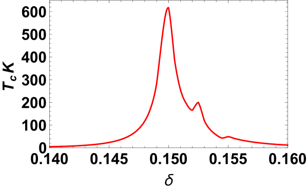
Figure 1: The superconducting transition temperature for the correlated model $T_{c}$ (Eq. (87)) ($t^{\prime}/t=-0.159,\;t^{\prime\prime}/t=0.01,\;\frac{m}{m^{*}}=Z$). The scale of the maximum transition temperature is smaller by an order of magnitude from the uncorrelated model. As the insulator is approached $\delta\to 0$, and $T_{c}$ decreases drastically. This is easy to understand since the quasiparticle weight $Z$ shrinks on approaching the insulating state, killing the coupling $g_{eff}$ Eq. (88). When $\delta$ goes beyond the peak (optimum) value, the effective superconducting coupling $g_{eff}$ agains falls off as seen in Fig. (2) and in Fig. (5) due to the other factors in Eq. (88). When $g_{eff}$ drops below $\sim 0.12$, the resulting $T_{c}$ is negligible.

In Fig. (1) the superconducting transition temperature for d-wave symmetry is shown as a function of the hole density $\delta=1-n$ where the band parameters are indicated in the caption. It shows that $T_{c}$ is maximum at $\delta\sim 0.15$ and falls off rapidly as one moves away from that density in either direction. The scale of $T_{c}$ is a few hundred K, which is an order of magnitude lower than that of the uncorrelated system. The small kink-like features to the right of the peak reflect structure in the DOS shown as inset in Fig. (2).

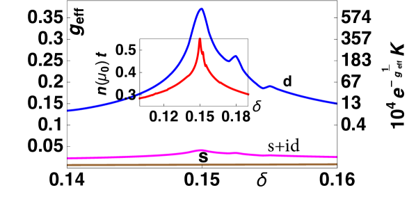
Figure 2: The figure and inset use $t^{\prime}/t=-0.159$, $t^{\prime\prime}/t=0.01$, and $\frac{m}{m^{*}}=Z$. The effective superconducting coupling $g_{eff}$ (Eq. (88)) for three Cooper pair symmetries: (i)(blue) d-wavefunction $\langle\left\{\cos(k_{x})-\cos(k_{y})\right\}^{2}\rangle_{FS}$, (ii)(brown) extended s-wavefunction $\langle\left\{\cos(k_{x})+\cos(k_{y})\right\}^{2}\rangle_{FS}$, and (iii)(magenta) $s+id$ wavefunction $\langle\left\{\cos^{2}(k_{x})+\cos^{2}(k_{y})\right\}\rangle_{FS}$. For the d-wavefunction, the drastic decrease of $T_{c}$ on both sides of the peak values in Fig. (1) can be understood by referring to the the second y-axis, giving the temperature scale $T_{c}^{appx}=10^{4}\times e^{-\frac{1}{g_{eff}}}$ K. This scale provides an order of magnitude of $T_{c}$ at a given $g_{eff}$ by assuming a prefactor $10^{4}$K. It illustrates the rapid reduction of $T_{c}$ when $g_{eff}\ {\raise-1.72221pt\hbox{$\buildrel<\over{\sim}$}}\ 0.12$. The other two symmetries lead to much smaller couplings and are therefore ineffective. Inset: The band DOS at the fermi energy shows an enhancement around the hole density $\delta=0.15$.

In Fig. (2) the effective superconducting coupling $g_{eff}$ is shown for three different symmetries of the Cooper pairs: $d$-wave, extended $s$-wave, and $s+id$-wave. It is clear that within this theory, only d-wave symmetry leads to robust superconductivity, the other two symmetries lead to effects too small to be observable.

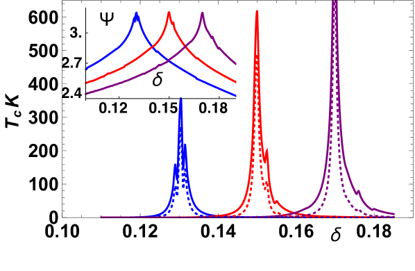
Figure 3: The superconducting transition temperature for the correlated model $T_{c}$ (Eq. (87)) for three parameter sets- (i) (red) $t^{\prime}/t$$=-0.159$, $t^{\prime\prime}/t$$=0.01$ with $\delta_{peak}=0.15$, (ii) (blue) $t^{\prime}/t$$=-0.137$, $t^{\prime\prime}/t=.01$ with $\delta_{peak}=0.13$ and (iii)(purple) $t^{\prime}/t$$=-0.181$,$t^{\prime\prime}/t$$=0.01$ with $\delta_{peak}=0.17$. The solid lines use $\frac{m}{m^{*}}=Z$ for and the dashed lines $\frac{m}{m^{*}}=3.4\delta$. Inset: $\Psi(\mu_{0})$ the fermi surface averaged d-wavefunction $\langle\left\{\cos(k_{x})-\cos(k_{y})\right\}^{2}\rangle_{FS}$ is shown for the three sets of band parameters. The peak values occur at the densities where $T_{c}$ is highest. Their peak magnitude $\sim 3.2$ indicates a strong constructive interference effect from $\vec{k}\sim\{\pm\pi,0\},\{0,\pm\pi\}$, where $|\cos(k_{x})-\cos(k_{y})|\sim 2$.

From Fig. (3) we see that the peak density is shifted by varying the band hopping parameters. As the peak density moves towards small $\delta$, its height falls rapidly. This is understandable as the effect of the quasiparticle weight $Z$ in the formulas Eqs. (87,88). We also note that the use of different expressions for the effective mass in Eqs. (92,93) change the width of the allowed regions somewhat, but are quite comparable.

The inset in Fig. (3) displays the d-wavefunction averages corresponding to the same sets of parameters. It is interesting to note that the height of the peaks $\Psi_{max}$$\sim$$3.2$ are close to their upper bound $4$, from a type of constructive interference that requires comment. Note first that the DOS can be expressed as a line integral in the octant of the Brillouin zone $n(\mu_{0})=\frac{2}{\pi^{2}}\int_{0}^{k_{max}}\frac{dk_{x}}{|v^{y}{(\vec{k})}|}$, where the velocity $v^{y}{(\vec{k})}=2\sin(k_{y})(t+2t^{\prime}\cos k_{x}+4t^{\prime\prime}\cos k_{y})$ is evaluated with $k_{y}\to k_{y}(k_{x},\mu_{0})$ on the fermi surface. Thus the region of small $|v^{y}|$ dominates the integral. If $v^{y}$ vanishes on the fermi surface, we get a (logarithmic van Hove) peak in the DOS. Now the average of $\Psi(\mu_{0})$ is largest, when $\vec{k}$ is close to $\{\pm\pi,0\}$ and $\{0,\pm\pi\}$. Therefore if the fermi surface passes through $\{\pm\pi,0\}$ and $\{0,\pm\pi\}$ for an “ideal density”, then we simultaneously maximize the average of $\Psi$, and obtain a large $DOS$. The condition for this is found by equating the band energy at $\{\pm\pi,0\}$ to the chemical potential $\mu_{0}=4t^{\prime}-4t^{\prime\prime}$, thereby fixing the corresponding density $\delta$. It follows that a given $\delta$ can be found from several different sets of the parameters $t^{\prime},t^{\prime\prime}$. The inset of Fig. (3) shows the average $\Psi(\mu_{0})$ displays peaks, the middle one (red) coincides in location with the peak in the DOS in the inset of Fig. (2).

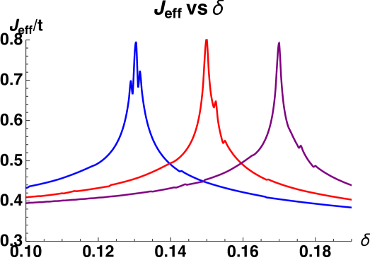
Figure 4: The effective exchange $J_{eff}$ from Eq. (89) for the three parameter sets- (i) (red) $t^{\prime}/t$$=\!-0.159$, $t^{\prime\prime}/t$$=0.01$ with $\delta_{peak}=0.15$, (ii) (blue) $t^{\prime}/t$$=\!-0.137$, $t^{\prime\prime}/t=.01$ with $\delta_{peak}$$=$$0.13$ and (iii)(purple) $t^{\prime}/t$$=\!-0.181$, $t^{\prime\prime}/t$$=0.01$ with $\delta_{peak}$$=$$0.17$. Since we assumed $J/t\sim 0.3$ (Eq. (89)), $J_{eff}/t$ is considerably enhanced in the range of densities exhibiting high $T_{c}$. This enhancement in turn boosts up $g_{eff}$, via Eq. (88), and hence plays an important role in giving an observable magnitude of $T_{c}$ in Fig. (1) and Fig. (3).

In Fig. (4) we illustrate the role of the feedback enhancement of the exchange $J$ due to the background spectral function discussed in Eq. (89).

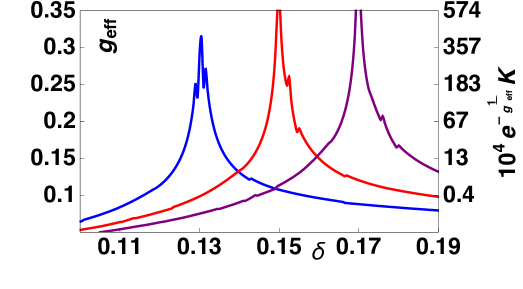
Figure 5: The effective superconducting coupling $g_{eff}$ (Eq. (88)) for the three curves in Fig. (3), with parameter sets- (i) (red) $t^{\prime}/t$$=-0.159$, $t^{\prime\prime}/t$$=0.01$ with $\delta_{peak}=0.15$, (ii) (blue) $t^{\prime}/t$$=-0.137$, $t^{\prime\prime}/t=.01$ with $\delta_{peak}=0.13$ and (iii)(purple) $t^{\prime}/t$$=-0.181$, $t^{\prime\prime}/t$$=0.01$ with $\delta_{peak}=0.17$. The drastic decrease of $T_{c}$ on both sides of the peak values in Fig. (3) can be understood by referring to the the second y-axis, giving the approximate temperature scale $T_{c}^{appx}=10^{4}\times e^{-\frac{1}{g_{eff}}}$ K.

For each set of parameters, there is a density region where both the DOS at the fermi energy and the averaged d-wavefunction are enhanced, and the confluence directly enhances $J_{eff}$. In turn this is reflected in the superconducting coupling $g_{eff}$. In Fig. (5) we see how the confluence of enhancements in the DOS and in the d-wavefunction $\Psi(\mu_{0})$, further boosts the superconducting coupling $g_{eff}$ and offsets to some extent the suppression due to a small magnitude of $Z$, as seen in Eq. (88). As a result of this competition $T_{c}$ turns out to be in the observable range. The additional y-axis in Fig. (5) translates the superconducting coupling $g_{eff}$ to an order of magnitude type transition temperature $T^{appx}_{c}=e^{-1/g_{eff}}\times 10^{4}\;K$. This scale helps us to understand why $T_{c}$ falls off so rapidly when $\delta$ increases beyond the peak value where the coupling $g_{eff}$ falls below $\sim 0.12$, thereby rapidly suppressing $T_{c}$.

5 Conclusions

This work presents a new methodology for treating extremely correlated superconductors. The exact equations of the normal and anomalous Greens functions in the superconductor are derived. These are further expanded in powers of a control parameter $\lambda$ related to the density of double occupancy, and the second order equations are given in Eqs. (51,52,54), together with the self consistency conditions Eqs. (25,41). A further simplification is possible for $T$$\sim$$T_{c}$ where the anomalous terms are small. This leads to a tractable condition for $T_{c}$ given in Eq. (69), expressed in terms of the electron spectral function. Further analysis uses a model spectral function Eq. (76), which is simple enough to yield an explicit expression for $T_{c}$ in Eq. (87). More elaborate calculations should be feasible upon the availability of reliable spectral functions, when one may directly solve Eq. (68).

Our calculation delineates the regime of parameters where superconductivity is possible in the  $t$-$J$  model within the ECFL theory. This regime turns out to be quite constrained. The calculation highlights the requirement of a substantial magnitude of the d-wavefunction average and the DOS at the fermi energy. It shows that $T_{c}$ is maximal at a density where $n(\mu_{0})$, the bare DOS is peaked, and is co-located with the peak of the fermi surface average of the d-wavefunction Eq. (71) (inset Fig. (3)). The latter aspect is understandable, since the passing of the Fermi level energy dispersion through the zone boundary points $\{\pm\pi,0\},\{0,\pm\pi\}$, promotes a peak in the DOS, and also leads to the maximization of $(\cos p_{x}-\cos p_{y})^{2}$. The prediction of a correlation between the peak in $T_{c}$ with a peak in the d-wavefunction average is testable, since the latter is amenable to measurement using angle resolved photoemission.

In the approximation used here, the maximum $T_{c}$ is nominally unbounded in a narrow density range here due to the logarithmic singularity of the DOS. It is expected to be cutoff to a finite value of ${\cal O}(10^{2}\mbox{K})$ due to a more exact integration over energies, when using a reliable spectral function, in the place of the model used here. Such an integration would also supersede the Gor’kov-type approximation of expanding around the fermi surface ($\int d\epsilon\;n(\epsilon)\sim n(\mu_{0})\int d\epsilon$) employed here, thereby flattening out the sharp peak into a smoother shape. Finally this mean-field description of the superconductor is expected to be corrected by fluctuations of the phase, in a strictly two dimensional case, and by interlayer coupling, in the physically realistic case of a three dimensional system of weakly coupled layers.

In conclusion this work contains the essential outline of a new formalism to treat superconducting states of models with extremely strong correlations, such as the  $t$-$J$  model. A transparent calculation within a low order approximation is presented here. It demonstrates that the exchange energy $J$ can indeed provide the fundamental binding force between electrons forming Cooper pairs. It leads to superconductivity with $T_{c}$’s of ${\cal O}(10^{2}\mbox{K})$, in a finite range of densities located away from the insulator, as also experimentally found in cuprate superconductors.

6 Acknowledgements:

The work at UCSC was supported by the US Department of Energy (DOE), Office of Science, Basic Energy Sciences (BES), under Award No. DE-FG02-06ER46319.

References

- [1] P. W. Anderson, Solid State Physics, edited by F. Seitz and D. Turnbull (Academic Press Inc,. New York, 1963), Vol 12, p.99; W. Kohn, Phys. Rev. 133, A171 (1964); A. B. Harris and R. V. Lange, Phys. Rev. 157, 295 (1967); W. F. Brinkman and T. M. Rice, Phys. Rev. B 2, 1324 (1970) (esp Eq. 4.1); K. A. Chao, J. Spalek and A. M. Oles, J. Phys. C 10, L271 (1977).
- [2] F.C. Zhang, T. M. Rice, Phys. Rev. B 37, 3759 (1988); B. S. Shastry, Phys. Rev. Letts. 63, 1288 (1989).
- [3] J. G. Bednorz and K. A. Muller, Z. Phys. B64, 188 (1986).
- [4] J. E. Hirsch, Phys. Rev. Letts. 54, 1317 ( 1985).
- [5] P. W. Anderson, Science 235, 1196 (1987).
- [6] G. Baskaran, Z. Zou and P. W. Anderson, Sol. St. Comm. 63, 973 (1987).
- [7] G. Kotliar, Phys. Rev. B37, 3664 (1988).
- [8] C. Gros, Ann. Phys. 189, 53 (1989).
- [9] H. Yokoyama and H. Shiba, J. Phys. Soc. Jpn. 57, 2482 (1988).
- [10] A. Paramekanti, M. Randeria and N. Trivedi, Phys. Rev. Lett. 87, 217002, (2001).
- [11] C.S. Hellberg and E.J. Mele, Phys. Rev. Lett. 67, 2080 (1991).
- [12] F.C. Zhang, T.M. Rice, Phys. Rev. B 37, 3759 (1988).
- [13] T. Giamarchi and C. Lhuillier, Phys. Rev. B 43, 12943 (1991).
- [14] M. Ogata and H. Fukuyama, Rep. Prog. Phys. 71, 036501 (2008).
- [15] T.-S. Huang, C. L. Baldwin, M. Hafezi, V. Galitski, arXiv:2004.10825 (2020).
- [16] S. Banerjee, T. V.Ramakrishnan and C. Dasgupta, Phys. Rev. B 83, 024510 (2011); Phys. Rev. B 84, 144525 (2011).
- [17] B. S. Shastry, Phys. Rev. Letts. 107, 056403 (2011). http://physics.ucsc.edu/~sriram/papers/ECFL-Reprint-Collection.pdf
- [18] B. S. Shastry, Ann. Phys. 343, 164-199 (2014).
- [19] F. J. Dyson, Phys. Rev. 102, 1217 (1956); S.V. Maleev, Sov. Phys. JETP 6, 776 (1958).
- [20] T. Holstein and H. Primakoff, Phys. Rev. 58, 1098 (1940).
- [21] B. S. Shastry, Phys. Rev. B 87, 125124 (2013).
- [22] J M Luttinger and J C Ward, Phys. Rev. 118, 1417 (1960); J. M. Luttinger, Phys. Rev. 119, 1153 (1960).
- [23] B S Shastry, Ann. Phys. 405,155 (2019).
- [24] A Damascelli, Z Hussain, and Z-X Shen, Rev. Mod. Phys. 75, 473 (2003).
- [25] F. J. Dyson, Phys. Rev. 75, 486 (1949).
- [26] A. Georges, G. Kotliar, W. Krauth, and M. J. Rozenberg, Rev. Mod. Phys. 68, 13 (1996); W. Metzner and D. Vollhardt, Phys. Rev. Lett. 62, 324 (1989).
- [27] R. Zitko, D. Hansen, E. Perepelitsky, J. Mravlje, A. Georges, and B. S. Shastry, Phys. Rev. B 88 235 132 (2013).
- [28] B S Shastry and E Perepelitsky, Phys. Rev. B 94 045138 (2016).
- [29] B. S. Shastry and P. Mai, Phys. Rev. B101,115121(2020).
- [30] B. S. Shastry and P. Mai, arXiv:1703.08142, New Jour. Phys. 20 013027 (2018).
- [31] P. Mai and B. S. Shastry, arXiv:1808.09788; Phys. Rev. B98, 205106 (2018)
- [32] G.-H. Gweon, B. S. Shastry and G. D. Gu, Phys. Rev. Letts. 107, 056404 (2011).
- [33] L. P. Gor’kov, Sov. Phys. JETP 7, 505 (1958).
- [34] G. M. Eliashberg, Soviet Physics JETP 11, 696 ( 1960).
- [35] A. B. Migdal, Soviet Physics JETP 34, 996 (1958)
- [36] C. C. Tsuei, J. R. Kirtley, M. Rupp, J. Z. Sun, A. Gupta, M. B. Ketchen, C. A. Wang, Z. F. Ren, J. H. Wang, and M. Bhushan, Science, 271, 329 (1996).
- [37] D. J. Scalapino, Phys. Repts. 250, 329 (1995).
- [38] M. Gutzwiller, Phys. Rev. Letts. 10, 159 (1963).
- [39] J. Hubbard, , Proc. R. Soc. London, Ser. A 277, 237 (1964).
- [40] Hubbard Operators in the Theory of Strongly Correlated Electrons, S. G. Ovchinnikov, V. V. Val’kov, Imperial College Press, London (2004)
- [41] E. Perepelisky and B. S. Shastry, Ann. Phys. 357, 1 (2015).
- [42] S. Tomonaga, Prog. Theor. Phys. 1, 27 (1946).
- [43] J. Schwinger, Phys. Rev. 74, 1439 (1948).
- [44] P. C. Martin and J. Schwinger, Phys. Rev. 115, 1342 (1959).
- [45] S. Engelsberg, Phys. Rev. 126, 1251 (1962).
- [46] L. D. Landau, Sov. Phys. J.E.T.P. 30, 1058 (1956),ibid 32, 59
- [47] P. Nozières, in Theory of Interacting Fermi Systems, (W. A. Benjamin, New York, 1964).
- [48] A. A. Abrikosov, L. Gor’kov and I. Dzyaloshinski, Methods of Quantum Field Theory in Statistical Physics , Prentice-Hall, Englewood Cliffs, NJ (1963).
- [49] W.F. Brinkman and T.M. Rice, Phys. Rev. B 2, 4302 (1970).
- [50] T. Yoshida, T. Yoshida, X. J. Zhou, D. H. Lu, S. Komiya, Y. Ando, H. Eisaki, T. Kakeshita, S. Uchida, Z. Hussain, Z.-X. Shen, and A. Fujimori, J. Phys.: Condens. Matter 19, 125209 (2007); M. Hashimoto, T. Yoshida, H. Yagi, M. Takizawa, A. Fujimori, M. Kubota, K. Ono, K. Tanaka, D. H. Lu, Z.-X. Shen, S. Ono, and Y. Ando, Phys. Rev. B 77, 094516 (2008).
- [51] R. R. P. Singh, P. A. Fleury and K. Lyons, Phys. Rev. Letts. 62, 2736 (1989).
- [52] For this purpose we could, in principle use the Sommerfeld type low T formula for a fermi liquid. Estimating from data turns out to be somewhat problematic. One must not only choose the bare band hopping parameters, but also neglect features of the data, such as the strong dependence of the Sommerfeld coefficient in the data for , as reported in J. W. Loram, J. Luo, J. R. Cooper, W. Y. Liang and J.L. Tallon, J. Phys. C Solids 62 59 (2001).