A Comparison of Circumgalactic Mgii Absorption between the TNG50 Simulation and the MEGAFLOW Survey
Abstract
The circumgalactic medium (CGM) contains information on gas flows around galaxies, such as accretion and supernova-driven winds, which are difficult to constrain from observations alone. Here, we use the high-resolution TNG50 cosmological magnetohydrodynamical simulation to study the properties and kinematics of the CGM around star-forming galaxies in halos at using mock Mgii absorption lines, which we generate by postprocessing halos to account for photoionization in the presence of a UV background. We find that the Mgii gas is a very good tracer of the cold CGM, which is accreting inward at inflow velocities of up to . For sight lines aligned with the galaxy’s major axis, we find that Mgii absorption lines are kinematically shifted due to the cold CGM’s significant corotation at speeds up to 50% of the virial velocity for impact parameters up to 60 kpc. We compare mock Mgii spectra to observations from the MusE GAs FLow and Wind (MEGAFLOW) survey of strong Mgii absorbers ( Å). After matching the equivalent-width (EW) selection, we find that the mock Mgii spectra reflect the diversity of observed kinematics and EWs from MEGAFLOW, even though the sight lines probe a very small fraction of the CGM. Mgii absorption in higher-mass halos is stronger and broader than in lower-mass halos but has qualitatively similar kinematics. The median-specific angular momentum of the Mgii CGM gas in TNG50 is very similar to that of the entire CGM and only differs from non-CGM components of the halo by normalization factors of .
1 Introduction
The accretion of gas onto disk galaxies is a fundamental part of galaxy formation and evolution, as gas within disks is continually used to form stars and must therefore be regularly replenished (e.g., Putman, 2017). All such gas, whether pristine gas from cosmological inflows or recycled gas in the process of reaccreting, must pass through the local environment surrounding galaxies, often called the circumgalactic medium (CGM). The CGM might contain a substantial amount of angular momentum as shown by many studies of galaxy simulations (e.g., Stewart et al., 2011; Danovich et al., 2015; DeFelippis et al., 2020). As the gas accretes onto the galaxy, the angular momentum will flow inward too, meaning the CGM is a source not just of the mass of the disk, but its angular momentum as well.
Not all gas surrounding galaxies is inflowing though: the CGM also contains outflowing gas ejected from the galaxy by feedback from supernovae and active galactic nuclei (AGN), which is capable of affecting the way in which CGM gas eventually joins the galaxy (DeFelippis et al., 2017). All of these physical processes occur concurrently and result in a multiphase environment shown in observations to have complex kinematics (see Tumlinson et al., 2017, and references therein).
A large number of recent observations of the CGM have been accomplished through absorption line studies of background quasars through dedicated surveys (e.g., Liang & Chen, 2014; Borthakur et al., 2015; Kacprzak et al., 2015). For instance, some surveys are constructed by cross-correlating quasar absorption lines with spectroscopic redshift surveys such as the Keck Baryonic Structure Survey (KBSS; Rakic et al., 2012; Rudie et al., 2012; Turner et al., 2014) or with photometric surveys like the Sloan Digital Sky Survey (SDSS; Huang et al., 2016; Lan & Mo, 2018; Lan, 2020). Other CGM surveys attempt to either match individual absorption lines to known galaxies (i.e., are “galaxy selected”), like the COS-Halos (e.g., Tumlinson et al., 2011; Werk et al., 2013; Borthakur et al., 2016; Burchett et al., 2019), COS-LRG (Chen et al., 2018; Zahedy et al., 2019), and the low-redshift Keck surveys conducted at Keck Observatory (Ho et al., 2017; Martin et al., 2019), or match galaxies near known absorbers (i.e., “absorber selected”) such as the MusE GAs FLOw and Wind survey (MEGAFLOW; Schroetter et al., 2016, 2019, 2021; Wendt et al., 2021; Zabl et al., 2019, 2020, 2021). In these surveys, there is generally only one quasar sight line per galaxy, but in certain rare cases it is possible to find multiple sight lines associated with a single galaxy through multiple quasars (Bowen et al., 2016), a single multiply lensed quasar (Chen et al., 2014; Zahedy et al., 2016; Kulkarni et al., 2019), an extended lensed quasar (Lopez et al., 2018), or even an extended background galaxy (Diamond-Stanic et al., 2016).
The Mgii ion has been a focus of many recent surveys including the Mgii Absorber-Galaxy Catalog (MAGIICAT; Chen & Tinker, 2008; Chen et al., 2010a; Nielsen et al., 2013b, a, 2015), the Magellan MagE Mgii (M3) Halo Project (Chen et al., 2010a, b; Huang et al., 2021), the MUSE Analysis of Gas around Galaxies Survey (MAGG; Dutta et al., 2020), the PRIsm MUlti-object Survey (PRIMUS; Coil et al., 2011; Rubin et al., 2018), and the aforementioned MEGAFLOW survey, as well as individual absorbers (e.g., Lopez et al., 2020). These studies belong to a long history of Mgii absorption line surveys (e.g., Bergeron & Boissé, 1991; Bergeron et al., 1992; Steidel & Sargent, 1992), which unveiled the first galaxy–absorber pairs at intermediate redshifts. Though not the focus of this paper, Mgii has also been seen in emission in extended structures around the galaxy and in the CGM (e.g., Rubin et al., 2011; Rickards Vaught et al., 2019; Rupke et al., 2019; Burchett et al., 2021; Zabl et al., 2021).
Along with this wealth of Mgii observations, researchers in recent years have found Mgii kinematics to be correlated over large spatial scales. In particular, both Bordoloi et al. (2011) and Bouché et al. (2012) found a strong dependence of Mgii absorption on azimuthal angle: specifically, more absorption near and and a lack of absorption near . This type of absorption distribution is generally interpreted as bipolar outflows along the minor axis and inflows along the major axis. In this context, both galaxy-selected (e.g., Ho et al., 2017; Martin et al., 2019) and absorption-selected Mgii studies (e.g., Kacprzak et al., 2012; Bouché et al., 2013, 2016; Zabl et al., 2019) have given support to the interpretation of accretion of gas from the CGM onto the galaxy. These Mgii studies show that when sight lines are located near the major axis of the galaxy there are clear signatures of corotating cold gas with respect to the galaxy kinematics.
However, despite such extensive observational data, developing a general understanding of cold gas in the CGM from the Mgii line alone remains difficult due to the limited spatial information provided by the observational technique (though IFU mapping of lensed arcs in Lopez et al., 2020, e.g.,, Mortensen et al., 2021, and Tejos et al., 2021 can improve this in the future), as well as the fact that Mgii gas may not be representative of the entire cold phase of the CGM. To study more physically fundamental properties of the CGM, it is therefore necessary to turn to galaxy simulations.
In cosmological simulations (see Vogelsberger et al., 2020 for a review), the CGM has been notoriously difficult to model accurately due to the need to resolve very small structures (e.g., Hummels et al., 2019; Peeples et al., 2019; Suresh et al., 2019; Corlies et al., 2020). Nonetheless, the CGM has been shown to preferentially align with and rotate in the same direction of the galaxy, especially near the galaxy’s major axis (Stewart et al., 2013, 2017; Ho et al., 2019; DeFelippis et al., 2020), which is qualitatively consistent with observations in the same spatial region of the CGM (e.g., Zabl et al., 2019). However, this general qualitative agreement between simulations and observations is difficult to put on firm ground quantitatively due to the inherent differences between observations and simulations.
In this paper, we analyze a set of halos from the TNG50 simulation (Nelson et al., 2019; Pillepich et al., 2019) using the Trident tool (Hummels et al., 2017) to model the ionization state of the CGM and then perform a quantitative comparison of the kinematics of the cool () CGM traced by Mgii absorption to major-axis sight lines from the MEGAFLOW survey (Zabl et al., 2019) while attempting to match the observational selection criteria as described in Section 2. We note that our comparison to MEGAFLOW galaxies with stellar masses is complementary to that of both Nelson et al. (2020), who study the origins of cold CGM gas of very massive galaxies (), and Nelson et al. (2021), who study properties of extended Mgii emission in the CGM.
The paper is organized as follows. In Section 2, we describe the TNG50 simulation and MEGAFLOW sample used in the comparison, and we outline the analysis pipeline used to generate mock observations. In Section 3, we describe our main results, first by comparing the simulated and real observations, then by analyzing the features of the simulation that give rise to the properties of the mock observations. In Section 4, we discuss the implications of our results for the role of the CGM in galaxy formation, and we summarize our findings in Section 5.
2 Methods
2.1 Simulations
We utilize the TNG50 simulation (Nelson et al., 2019; Pillepich et al., 2019), the highest-resolution version of the IllustrisTNG simulation suite (Marinacci et al., 2018; Naiman et al., 2018; Nelson et al., 2018; Pillepich et al., 2018; Springel et al., 2018), which is itself based on the original Illustris simulation (Vogelsberger et al., 2014a, b). TNG50 evolves a periodic box from cosmological initial conditions to with the moving-mesh code Arepo (Springel, 2010; Weinberger et al., 2020). It has a baryonic mass resolution of per cell, which is a factor of better than the resolution of TNG100. We discuss the effect of simulation resolution on our results later in Section 3.
2.2 Observational Data
The MEGAFLOW survey (N. Bouché et al., in preparation) consists of a sample of 79 Mgii absorbers in 22 quasar lines of sight observed with the Multi-Unit Spectroscopic Explorer (MUSE; Bacon et al., 2006). The quasars were selected to have at least three Mgii absorbers from the Zhu & Ménard (2013) SDSS catalog in the redshift range such that the [Oii] galaxy emission lines fell within the MUSE wavelength range (). A threshold on the rest-frame equivalent width of was also imposed on each absorber.
For this paper, we focus on a preliminary subset of the MEGAFLOW sample of Mgii absorber–galaxy pairs whose quasar location is positioned within 35∘ of the major axis of the host galaxy (Zabl et al., 2019). This subset consists of nine absorber–galaxy pairs with redshifts and impact parameters () ranging from 13 to 65 kpc with a mean of kpc. Zabl et al. (2019) found that the Mgii gas in these absorbers show a strong preference for corotation with their corresponding host galaxies.
The galaxies in Zabl et al. (2019) are both fairly isolated by having at most one companion within , and star forming with [Oii] fluxes , i.e., star-formation rates . The galaxies have stellar masses ranging from and halo masses ranging from , where is defined from the stellar mass–halo mass relation from Behroozi et al. (2010). As Zabl et al. (2019) show, these halo masses generally match the Bryan & Norman (1998) definition of .
2.3 Sample selection and Forward Modeling
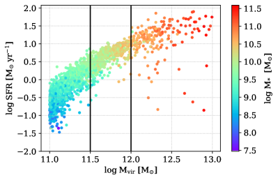
Figure 2 shows the central galaxies’ instantaneous star formation rates (SFR) and stellar masses of all TNG50 halos in and around the mass range of interest. Since we aim to compare the Mgii absorption properties of mock line-of-sight (LOS) observations through TNG50 halos to those of major-axis sight lines of the MEGAFLOW survey, we first select a sample of simulated halos at in the mass range using the Bryan & Norman (1998) definition for , which results in a sample of 495 halos. In the remainder of this paper, we will refer to this subsample as the “fiducial” sample. The chosen redshift is typical for the Zabl et al. (2019) sample, and the halo mass range covers the typical inferred virial masses of their halos. Nearly all of the halos in our fiducial sample host central galaxies with SFR and stellar masses of , which is consistent with the MEGAFLOW subsample as described in Section 2.2.
For each halo, we adjust all velocities to be in the center-of-mass frame of the stars in the central galaxy, and we rotate it so that the stellar specific angular momentum of the central galaxy points in the -direction (the - and -directions are both arbitrary). With this geometry we then define a sight line in the plane by the impact parameter , the azimuthal angle , and the inclination angle , where is the projected distance from the center of the galaxy in the plane (i.e., “sky” plane), is the angle above the rotational plane of the galaxy, and is the angle of the sight line with respect to the sky plane. In this setup, edge-on and face-on views have and , respectively (see Figure 1 of Zabl et al., 2019 for a sketch of the geometry described here). In order to mimic the observations of Zabl et al. (2019), we select sight lines through each halo at values of ranging from to , and , and at , representing the average inclination angle of a random sight line.
In order to generate observations of our TNG50 sample, we use the Trident package (Hummels et al., 2017), which calculates ionization parameters for outputs of galaxy simulations using properties of the simulated gas cells and Cloudy (Ferland et al., 2013) ionization tables. These tables take as input the gas temperature, density, metallicity, and cosmological redshift of each gas cell and provide ionization fractions and number densities of desired ions. We make use of the current development version of Trident111http://trident-project.org (v1.3), which itself depends on the current development version of yt222https://yt-project.org (v4.0). In this paper, we use a set of ion tables created assuming collisional ionization equilibrium, photoionization from a Faucher-Giguère et al. (2009) UV background, and self-shielding of neutral hydrogen (for details see Emerick et al., 2019 and Li et al., 2021), as this was the background radiation model used to evolve the TNG50 simulation. We also use the elemental abundance of magnesium in each gas cell tracked by the simulation rather than assuming a constant solar abundance pattern throughout the halo to achieve greater self-consistency with TNG50. We note, however, that our results are not particularly sensitive to either of these choices.
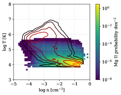
Since our focus is on the Mgii line, we show in Figure 4 a temperature–density phase diagram of the gas in one of the TNG50 halos from our sample, colored by the Mgii mass probability density. From this plot, it is clear that Mgii is mostly formed from the coldest () and densest () gas in the halo, though some Mgii mass exists at a larger range of temperatures and densities. However, contours showing the total gas mass demonstrate that despite this large range in temperature and density, essentially none of the diffuse “hot” phase, comparable in mass to the cold phase, contributes to Mgii absorption. We also note here that for this analysis we are excluding star-forming gas as its temperature and density are defined using an effective equation of state (Springel & Hernquist, 2003) and are therefore not analogous to the physical properties of non-star-forming gas. Properly modeling the physical properties of the star-forming gas (see Ramos Padilla et al., 2021 for an example of this technique) introduces a level of complexity not necessary for this analysis: we find that our results are not affected by the exclusion of this gas since our sight lines through the CGM rarely intersect any star-forming gas cells as most of them are within the galactic disk.
3 Results
We first present in Section 3.1 the results of directly comparing the Mgii properties of TNG50 and MEGAFLOW using the analysis described in Section 2. Then, we further analyze the 3D kinematic properties of the Mgii-bearing gas from TNG50 in Section 3.2 and consider evolution of Mgii absorption properties with halo mass and simulation resolution in Section 3.3.
3.1 Comparing TNG50 to MEGAFLOW
In Figure 5, we show Mgii column density maps of a selection of TNG50 halos drawn from our fiducial sample at . The halos are aligned so that the angular momentum vector of the stars in the central galaxy points along the vertical axis; thus, the view is edge-on. The strongest Mgii columns are found within and very close to the galaxy, demarcated by a red circle with a radius of twice the galaxy’s stellar half-mass–radius (the same definition used in DeFelippis et al., 2020). Beyond the galaxy, Mgii gas consistently appears to both surround the galactic disk and be very clumpy, but the amount and morphology of such gas varies greatly. In particular, there is significant variation with azimuthal angle: the highest Mgii columns generally appear in the plane of rotation, but strong columns can occur above and below the disk as well, such as in halo 265 (the bottom left panel of Figure 5). Péroux et al. (2020) found the CGM gas metallicity to vary with azimuthal angle, but interestingly, they found gas near the major axis to have lower than average metallicity in the halo, indicating that large Mgii columns do not necessarily correspond to metal-enriched gas. High Mgii columns are much less common in the outer halo (), but the presence of satellite galaxies can populate that region with Mgii gas, shown most clearly in halo 340 (the bottom right panel of Figure 5).
Within our fiducial sample, it is evident that the distribution of Mgii varies drastically, presumably due to different halo formation histories. Sight lines through different halos will therefore likely produce different absorption profiles even for sight lines with identical geometries. This highlights the necessity of calculating population averages of Mgii properties from TNG50 to compare to MEGAFLOW.
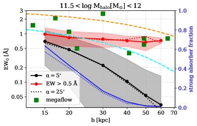
We begin such a comparison with Figure 7, which shows the average strength of Mgii absorption, represented as the rest-frame equivalent width (EW0) as a function of impact parameter () for our fiducial sample. In this plot, we make an important distinction between the entire fiducial sample, shown in black, and the subset of “strong absorbers” in red. We define strong absorbers as sight lines through a halo that produce an absorption spectrum with EW (the same as in Zabl et al., 2019). It is this “absorber-selected” subset of the fiducial sample that is most directly comparable to MEGAFLOW. For easier comparison to Figure 5, we find that sight lines with EW have Mgii column densities ranging from , i.e., just above the lower limit of the color bar.
At all impact parameters, the average rest-frame EW of the “all absorbers” sample from TNG50 (black) is smaller than those of MEGAFLOW, as expected given the selection function. The difference ranges from a factor of only at to a factor of at . If, instead, we compare the average EW0 of the strong absorber subset (EW) from TNG50, which is the appropriate comparison to make, we find the mean shown in red. This is much more similar to the values from MEGAFLOW, especially for , but it is still as much as a factor of lower than the observed values at . However, the limited size and large scatter of the MEGAFLOW points from Zabl et al. (2019) make it difficult to assess the precise level of disagreement with TNG50. Sight lines at (solid) and (dotted) produce essentially identical equivalent widths over both the entire fiducial sample and the subset of strong absorbers. With the two additional dashed lines in Figure 7 we provide a point of comparison to larger samples of moderate-redshift Mgii absorbers from Nielsen et al. (2013a) and Lundgren et al. (2021). Though both of these samples have a slightly smaller equivalent-width threshold than Zabl et al. (2019) () and no selection based on the geometry of the sight line, they still bracket both the Zabl et al. (2019) absorbers and the strong absorbers from TNG50, indicating that these simulated Mgii EWs are also consistent with observed Mgii EWs in general, given the large scatter.
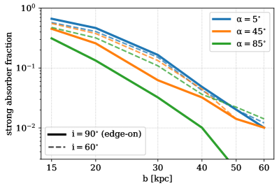
The blue lines in Figure 7 show the fraction of all sight lines that host strong absorbers as a function of impact parameter. At sight lines very close to the galaxy (), strong absorbers are common and in fact represent a majority of all halos. However, by the strong absorber fraction drops below 50%, and at the largest impact parameters shown, the fraction is only . Strong absorbers are slightly more common at compared to , which can be understood by noting that the sight lines with smaller pass through the disk midplane closer to the galaxy’s center, where gas is generally denser. However, this difference in strong absorber fraction does not affect the measured equivalent widths, indicating that the TNG50 halos’ agreement with MEGAFLOW for sight lines near the galaxies’ major axes is not subject to the precise geometries of the sight lines.
In Figure 9, we examine how Mgii EWs vary throughout the entire halo in TNG50, not just near the major axis, and we find a clear trend: at all impact parameters we study, the mean EW of a perfectly edge-on sight line decreases as the azimuth angle of that sight line increases. Sight lines near the minor axis (green) have EWs at least smaller than sight lines near the major axis (blue), and sight lines between both axes (orange) have EWs between the values at both axes. This represents a disagreement between TNG50 and Mgii observations, which are generally observed to have a bimodal distribution of near and (Bordoloi et al., 2011; Bouché et al., 2012; Kacprzak et al., 2012; Martin et al., 2019; Zabl et al., 2019; Lundgren et al., 2021). The distribution of in TNG50 is clearly peaked at small , implying that TNG50 is not producing the same kind of Mgii that is inferred to be outflowing in observations. It is also clear that this azimuthal angle dependence is very sensitive to the inclination angle of the sight line because it nearly disappears when the sight lines are inclined at an angle of with respect to the axis of rotation (dotted lines in Figure 9), as would be typical for observations. This sensitivity indicates that most Mgii absorption in TNG50 comes from a gas in the vicinity of the disk midplane, where we have already seen (Figure 7) that TNG50 is consistent with observations. Therefore, for the remainder of this paper we restrict our observational comparison to sight lines near the major axis.
Having established the degree of consistency of Mgii equivalent widths, we now examine kinematic signatures of Mgii along sight lines in TNG50 and compare them to MEGAFLOW. In Figure 10, we explicitly draw the connection between the Mgii gas cells that contribute to the column densities seen in Figure 5 and the velocity spectrum created from a subset of those cells that intersect a sight line through the halo. In each row, we show two orientations of one of the four halos from Figure 5 overlaid with a sight line with , , and , and the Mgii velocity spectrum generated from that sight line. From these few examples it is clear that the gas producing the Mgii absorption is generally not distributed uniformly along any sight line: it is usually concentrated in discrete clumps in regions of the sight line nearest to the galaxy. This is seen clearly in rows one, two, and four of Figure 10, where the majority of gas cells have positive LOS velocities (i.e., corotating with the galaxy) and produce distinct kinematic components in the spectrum that are often saturated.
It is also notable that by comparing the spectra alone it is possible to distinguish morphological differences in the Mgii distribution between halos. The first two halos, for example, have a prominent Mgii disk that both spectra reveal to be primarily corotating. The halo in row three, however, does not have such a clear disk, and the spectrum is instead composed of a cluster of counter-rotating gas cells significantly above the plane of the galaxy. The halo in row four has a spectrum with substantial corotating and counter-rotating components, which imply Mgii structure in between the ordered halos (rows one and two) and disordered ones (row three). With this small sample, we have demonstrated that the velocity spectrum, despite being composed of a very small fraction of all of the Mgii gas, is capable of reflecting the potential diversity of Mgii gas kinematics in halos of similar mass, but is also fairly consistent between halos with similar morphologies. Later in the paper, we consider whether the Mgii gas reflects the kinematics of other components of the CGM.
From these results, we now compare stacked spectra from the fiducial sample to the stacked spectra presented in Zabl et al. (2019). Figure 13 shows stacked spectra for the entire TNG50 fiducial sample (black), TNG50 strong absorbers (red), and the absorbers from Zabl et al. (2019) (green). The two panels correspond to two different impact parameters that allow a comparison between absorbers nearer to a galaxy and farther from a galaxy. In the left panel, showing stacked spectra at small impact parameters, there is a very clear kinematic picture. The strong absorber spectrum from TNG50 is symmetric, centered at , and has a with a full width at half maximum (FWHM) of , the same as the spectrum of Zabl et al. (2019). Thus, qualitatively, strong Mgii absorbers as a population generally have LOS velocities in the same direction as their corresponding galaxies’ rotations. One slight difference with the stacked spectra for strong absorbers is that the TNG50 spectrum (red) is somewhat shallower than the observed spectrum (green). However, there is essentially no difference between TNG50 spectra generated from sight lines at the two azimuthal angles (solid line) and (dotted line).
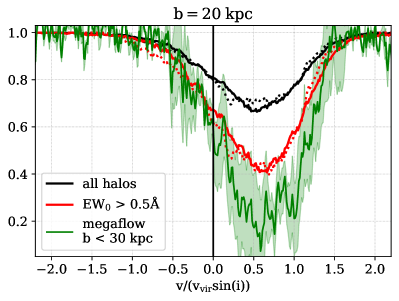

In Figure 13 (left), the only difference between the full fiducial spectrum and the strong absorber-only spectrum is the depth, indicating that, as a population, strong absorbers are not kinematically distinct from absorbers in general at this impact parameter. The precise reason for the discrepancy in the depth is difficult to determine, but it may be sensitive to certain parameters in the TNG physics model (e.g., metal loading of outflows from supernovae). However, it could also be an effect of simulation resolution (see Section 3.3). So, while TNG50 potentially slightly underproduces the observed amount of Mgii gas at 20 kpc, it does possess average kinematics that are consistent with observations of the same region of the CGM.
Figure 13 (right) compares the stacked spectra at a larger impact parameter ( kpc). The strong absorbers from TNG50 and MEGAFLOW (Zabl et al., 2019) are both shallower, wider (FWHMs of and respectively), no longer symmetric, and significantly noisier, though both are still approximately centered at a velocity on the order of . At this impact parameter, the depths of the simulated strong absorber and observed spectra are consistent with each other. However, strong absorbers no longer kinematically resemble the full fiducial sample: in addition to being much rarer at 40 kpc than at 20 kpc, the strong absorbers have larger positive velocities, indicating that Mgii in this region is tracing atypically faster-moving gas. As was the case at 20 kpc, the difference in the spectra between the two azimuth angles is minor. We also note here, but do not show, that the shapes and depths of individual spectra from Zabl et al. (2019) match quite well with particular individual spectra from the much larger fiducial sample from TNG50 (examples of individual spectra from TNG50 are shown in Figure 10).
3.2 3D Kinematics of Mgii in TNG50
In this section, we characterize the three-dimensional kinematics of the Mgii gas in TNG50 and its relation to the observed quantities we discussed in Section 3.1. We show average velocity profiles of the halos in the fiducial sample in Figure 15. The top panel shows the azimuthal velocity component () in spherical coordinates as a function of radius. We divide gas into cold and hot components based on a temperature threshold of K, which is chosen to separate the cold and hot clusters seen in Figure 4, although the profiles are not sensitive to the precise choice of temperature threshold. To understand the relationship of the hot and cold gas to Mgii-bearing material we also show the Mgii mass-weighted profiles.
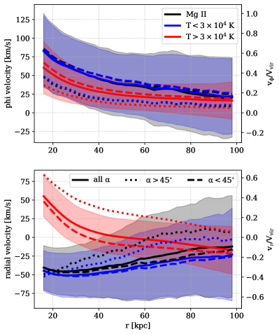
First, we see that the Mgii gas and the cold gas have nearly identical profiles throughout the halo. In the innermost regions of the CGM (, the cold gas has a mean azimuthal velocity of (), while in the outermost regions (, the mean azimuthal velocity decreases to (). At all radii, the scatter is quite large (), though the standard errors on this and all other mean velocities in Figure 15 range from only . Though not explicitly shown, most of the cold and Mgii gas mass is closer to the major rather than the minor axis because the all- profiles are much more similar to the (dashed) profiles than the (dotted) profiles. Hot gas has lower azimuthal velocities at all radii, a slightly shallower slope to its profile, and a smaller scatter in azimuthal velocity by a factor of but is otherwise qualitatively similar to the cold and Mgii gas. This relationship between hot and cold gas is consistent with similar measurements of made from TNG100 in DeFelippis et al. (2020).
In the radial-velocity profiles (Figure 15, bottom), we see a gulf between the velocities of the hot and cold gas develop within . Above this radius, the average radial velocities of all components of the gas converge to (), though the spread of radial velocities in this region of the CGM is very large, especially for cold gas ( scatter of ). Moving toward smaller radii, the cold gas inflow velocities become larger, while hot gas inflow velocities decrease and then switch to a net outflow at . The Mgii gas still traces the cold gas, which reaches typical inflowing velocities of in the inner CGM out to , where the spread in radial velocities is a factor of smaller than in the outer halo. The geometry of accretion and outflows is evident from this panel as well: hot gas has especially large mean outflowing velocities for while cold gas in the same region has a mean inflowing velocity in the inner halo and nearly no net radial motion in the outer halo. Most of the cold and Mgii gas mass is moving toward the galaxy in regions surrounding the major axis out to a substantial fraction of the virial radius. It is also clear that kinematically, Mgii gas in TNG50 is nearly identical to a simple cut on temperature and so is an excellent tracer of the kinematics of cold CGM gas. In the context of Section 3.1, these results indicate that mock Mgii spectra are representative of the entire cold phase of the CGM along the same sight lines.
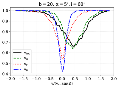
Finally, we examine the 3D velocities of the Mgii gas along our sight lines. In Figure 17, we plot stacked spectra for Mgii using the three spherical velocity components individually (, , and ), and compare those to the spectrum generated with the full velocity of our fiducial sample of halos. Both the and component spectra are centered at , indicating that over the entire sample they do not contribute any net velocity shift to the gas along the sight lines. The spectrum of the component is remarkably similar to the spectrum of the entire velocity, both in terms of velocity shift and width. This means that for our fiducial sample, the shape of the stacked velocity spectrum along sight lines is completely determined by only the (i.e., rotational) component of the velocity along those sight lines.
3.3 Effects of halo mass and resolution on Mgii in TNG50
We now describe how our main results vary with halo mass and mass resolution. To study the effect of halo mass, we consider two mass bins containing halos from TNG50 with and at , which are above and below the fiducial mass range and contain 1130 and 167 halos, respectively. As in Section 3.1 we calculate Mgii equivalent widths and generate velocity spectra that we show in Figure 20. For easier comparison, we also show the TNG50 fiducial sample.
As shown in the left panel of Figure 20, at a given impact parameter, the shape of the equivalent-width distribution changes with halo mass: lower halo masses (cyan) are much more likely to host weak or nonabsorbers than higher halo masses (magenta), and they are much less likely to host strong absorbers. We find this trend to hold at all impact parameters studied in this paper. We can see the effect on observability with the vertical lines in this panel, which show the mean equivalent widths of the strong absorbers in each mass bin. Typical strong absorbers in the fiducial sample have only slightly larger equivalent widths than those those at lower halo masses, but are substantially weaker than the strong absorbers at higher halo masses. At larger impact parameters, the mean equivalent widths of all strong absorbers is , but they are exceedingly rare in lower-mass halos. Thus, the primary effects of increasing halo mass on strong absorbers are to increase their occurrence at all impact parameters, especially at large distances, and to increase the mean equivalent width of strong absorbers for halo masses . We note that this result is qualitatively consistent with Chen et al. (2010b), who find a larger Mgii extent in the CGM of higher-mass galaxies.
Also shown in the left panel of Figure 20 is the equivalent-width distribution of 4315 halos with the same mass as the fiducial sample from the TNG100 simulation, which has a lower baryonic mass resolution than TNG50 by a factor of . Decreasing the simulation resolution lowers equivalent widths overall and steepens the distribution in the same way as decreasing the halo mass does, but the effect is weaker. The mean equivalent width of strong absorbers is largely unaffected by the change in resolution.
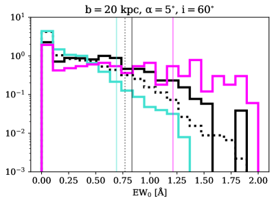
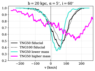
In the right panel of Figure 20 we examine the effect of halo mass and resolution on the observed Mgii spectrum of strong absorbers. We note that the spectra of the entire samples, as in Figure 13, have the same shape and center as their corresponding strong absorber subset, but are substantially shallower. We also plot the real velocity rather than the normalized velocity to emphasize the difference in equivalent widths, which can be more easily read off.
We see that the fiducial and lower-mass bins have remarkably similar spectra: they are both symmetric and centered at moderate positive velocities. The spectrum of the higher-mass bin is markedly different: it is much broader, asymmetric, and centered at a significantly higher velocity. It still, however, shows a preference for Mgii gas to be corotating. We note that the difference between Figure 20 as shown and the corresponding velocity-normalized spectrum (not shown) is that the normalized higher-mass spectrum is compressed slightly and therefore appears more similar to the normalized fiducial spectrum. Additionally, while the lower-mass and fiducial spectra are both centered at , the higher-mass spectra are peaked at . Higher halo masses () thus have substantially more Mgii absorption and more complex kinematic signatures than for the halo masses of the fiducial sample and lower.
Finally, we consider the difference that resolution makes in the Mgii absorption spectrum. As was the case with equivalent widths, the difference caused by resolution is smaller than the difference caused by either increasing or decreasing the halo mass. Apart from a slight change in the depth of the spectrum, the kinematic properties of strong absorbers in TNG are essentially resolution independent (see solid vs. dotted curves in Figure 20 for TNG50 and TNG100, respectively). The effect of increasing the resolution of the simulation is therefore primarily to increase the occurrence of strong absorbers at a given halo mass.
4 Discussion
4.1 The Role of Mgii in TNG
We consider here the ramifications of the detailed analysis of Mgii in TNG from Section 3. In Figure 15, we found that Mgii gas is very well approximated by a simple temperature cut. Therefore, we expect the angular momentum of cold gas in the CGM of TNG galaxies should be very similar to that of Mgii. DeFelippis et al. (2020) found cold CGM gas in halos of this mass range and redshift to have higher angular momentum when surrounding high-angular-momentum galaxies, meaning Mgii is likely tracing high-angular-momentum gas in the CGM of these halos. As the velocity spectrum’s center and shape is almost completely set by the rotational velocity component (see Figure 17), it should therefore be possible to use Mgii velocity spectra from sight lines near the major axis to estimate the angular momentum of cold gas in the CGM.
In Section 3.3 we examined possible halo mass and resolution dependencies of our results with two main goals in mind: to establish any broad effects of the TNG feedback model on Mgii, and to determine to what extent the cosmological simulation can capture Mgii kinematics. Feedback is known to be important for regulating gas flows into, out of, and around galaxies, and therefore could have observable signatures in the Mgii spectra, especially at different halo masses. The results of the halo mass analysis suggest that for halos with masses between and , the physical mechanisms affecting their CGM are similar enough to result in Mgii spectra that essentially scale with the halo’s virial velocity. This is presumably because feedback from supernovae is the dominant form of feedback that affects the CGM for all halo masses below and produces Mgii gas with similar kinematic signatures. For halos above however, Mgii gas has stronger overall absorption, as reflected by their flatter EW distribution, and substantially larger velocities and velocity dispersions, as reflected by their very broad velocity spectra. This is likely due to the dominant form of feedback switching from stars to AGN around this halo mass. However, within the higher-mass sample, halos with larger black hole masses do not themselves have broader Mgii spectra, so there is probably a combination of effects that result in a noticeable difference in the properties of the spectrum at higher masses.
Nelson et al. (2020) have recently used TNG50 to study the origin of cold Mgii gas in the CGM of very massive () galaxies and found structures of size a few that are sufficient to explain the observed covering fractions and LOS kinematics. They also note that while some fundamental properties like the number of cold gas clouds present in halos are not converged at TNG50’s resolution, the total cold gas mass of such halos is converged in TNG50. This supports our findings that our kinematic results do not qualitatively change even going from TNG50 to TNG100, a factor of in mass resolution (Figure 20), because the majority of the Mgii mass is already in the halo by TNG50’s resolution. We expect higher-resolution simulations to produce more strong absorbers at a given halo mass but the rotation of Mgii near the major axis appears to be a resolution-independent aspect of the CGM for MEGAFLOW analogs in the TNG simulations.
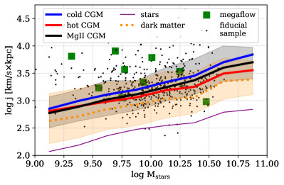
Finally, in Figure 22, we show the specific angular momentum () of different halo components as a function of stellar mass of their central galaxies, with the goal of contextualizing the angular momentum of Mgii gas (black line) in the CGM in relation to the rest of the gas in the CGM as well as to the other components of the halo. The slope of this relation for the stellar component of galaxies (purple line) is as generally observed (e.g., Fall & Romanowsky, 2013), and all other components appear to have roughly equal slopes. Most interesting are the relative positions of the CGM and dark matter (orange line) on this plane. At a given stellar mass, all components of the CGM have a slightly higher typical than that of the dark matter by . There are multiple potential reasons for this. First, galaxies can remove low-angular-momentum gas from the CGM by accreting it and using it to form stars. Second, feedback from stars and/or AGN can also eject low-angular-momentum gas from the halo completely. Finally, dark matter in the halo can transfer some of its angular momentum to the gas. Regardless, it is clear that Mgii traces the angular momentum of the both the cold and hot components of the CGM quite well.
Also shown in Figure 22 are two sets of points representing Mgii gas in individual halos: the fiducial sample in black and the Zabl et al. (2019) sample in green, for which was estimated using their derived rotational velocities. The two are not directly comparable since the points from Zabl et al. (2019) represent Mgii gas along a single sight line, yet they are still able to reproduce the scatter in this relation found in TNG50, though they are somewhat biased toward higher . This bias is likely due to the selection in Zabl et al. (2019) of strong Mgii absorption near the major axis, which is where high- cold gas tends to reside in the CGM as shown in DeFelippis et al. (2020). Nevertheless, from Figure 22 we can conclude that estimations of the angular momentum content of the CGM provided by single sight lines of Mgii can get within of typical values from TNG50 over a large range of galaxy masses.
4.2 Comparisons to Recent Work
We now highlight results from previous work on Mgii absorption in observations and simulations in the context of our results. Observations of Mgii using sight lines near the major axis of galaxies have generally found that gas is corotating with the galaxy both for small impact parameters of (e.g., Bouché et al., 2016) and large impact parameters of (e.g., Martin et al., 2019). Using a lensed system, Lopez et al. (2020) observed multiple sight lines of the same CGM and measured a decreasing Mgii rotation curve that is qualitatively similar to Figure 15. However, their absorption data only go out to . Our work suggests Mgii rotation curves should continue to decrease to at least 100 kpc, though based on the maps in Figure 5 the Mgii column densities at those distances are significantly below current observational limits.
While this paper is focused on Mgii gas near the major axis, there are also recent results suggesting Mgii outflows along the minor axis of galaxies with velocities (e.g., Schroetter et al., 2019; Zabl et al., 2020). It is worth noting though that Mortensen et al. (2021) found a lensed system with Mgii on the geometric minor axis of the absorber galaxy with LOS velocities and a large velocity dispersion, indicating that the kinematics of Mgii outflows may vary significantly. We showed in Figures 9 and 15 that Mgii absorption along the minor axis is weaker than along the major axis, and that there are no net Mgii outflows along the minor axis in the TNG fiducial sample. This result appears to be discrepant with the previously cited observational papers, but we defer a detailed analysis to a future paper.
Ho et al. (2020) recently studied similar aspects of Mgii absorption in the EAGLE simulation at and found results broadly consistent with ours. Specifically, they measure a rotating Mgii structure around star-forming galaxies as well as a lower detection fraction of Mgii near the minor axis. They also find that higher-mass galaxies host detectable (i.e., above a fixed column density) Mgii structures out to larger distances in the CGM, which we indirectly show with the EW distributions in Figure 20, where higher-mass halos have more strong absorbers.
5 Summary
We have simulated Mgii absorption in the CGM of halos from TNG50 comparable to the major-axis sight lines observed in the MEGAFLOW survey by Zabl et al. (2019) and compared absorption and kinematic properties of the two samples. We also examined the 3D kinematics of the Mgii in TNG50. Our conclusions are as follows:
- 1.
-
2.
A majority of halos are strong absorbers at the smallest impact parameter studied (15 kpc), but the strong absorber fraction drops quickly as a function of distance (Figure 7).
-
3.
The stacked velocity spectra of TNG50 strong absorbers match the stacked spectra of Zabl et al. (2019) very well, thus supporting the physical interpretation of corotation both below 30 kpc, where the spectra are strongly peaked near and symmetric, and above 30 kpc, where the spectra are similarly peaked but are much noisier, broader, and asymmetric (Figure 13).
-
4.
In TNG50, Mgii gas has velocity profiles nearly identical to gas below a temperature cutoff of , meaning Mgii absorption is a good proxy for cold gas kinematics in general. There is substantial rotation and typical inflow velocities of up to out to in the CGM (Figure 15).
-
5.
The radial and polar velocity components by themselves do not cause any net velocity shift in the stacked spectrum, which implies that Mgii absorption kinematics alone cannot be used to measure typical inflow speeds of rotating gas in the CGM. (Figure 17).
-
6.
Mgii absorption strengths and spectra are stronger and broader for halos more massive than the fiducial sample of halos but do not change very much for halos less massive than the fiducial sample. Lowering the resolution from TNG50 to TNG100 only modestly changes any of the Mgii kinematic properties (Figure 20).
-
7.
The median-specific angular momentum of the Mgii component of the CGM as a function of galactic stellar mass is very similar to that of both cold and hot CGM gas, and it is larger than that of the dark matter halo and the stars in the galaxy by and , respectively. Estimates of the specific angular momentum of Mgii from the Zabl et al. (2019) data are also reasonably close to the values from TNG50 to within a factor of . (Figure 22).
This work demonstrates that generating mock Mgii observations from TNG50 generates absorption spectra that are comparable to real data. In particular, our results are consistent with the emerging picture of rotating Mgii gas found in observations and also other simulations. In future work, we plan to widen our investigation to include other ions that trace warmer and more diffuse gas, as well as follow gas at particular redshifts backward and forward through time to determine the stability of various ion structures and their role in transporting angular momentum to or from the galaxy.
References
- Bacon et al. (2006) Bacon, R., Bauer, S., Boehm, P., et al. 2006, in Society of Photo-Optical Instrumentation Engineers (SPIE) Conference Series, Vol. 6269, Society of Photo-Optical Instrumentation Engineers (SPIE) Conference Series, ed. I. S. McLean & M. Iye, 62690J, doi: 10.1117/12.669772
- Behroozi et al. (2010) Behroozi, P. S., Conroy, C., & Wechsler, R. H. 2010, ApJ, 717, 379, doi: 10.1088/0004-637X/717/1/379
- Bergeron & Boissé (1991) Bergeron, J., & Boissé, P. 1991, A&A, 243, 344
- Bergeron et al. (1992) Bergeron, J., Cristiani, S., & Shaver, P. A. 1992, A&A, 257, 417
- Bordoloi et al. (2011) Bordoloi, R., Lilly, S. J., Knobel, C., et al. 2011, ApJ, 743, 10, doi: 10.1088/0004-637X/743/1/10
- Borthakur et al. (2015) Borthakur, S., Heckman, T., Tumlinson, J., et al. 2015, ApJ, 813, 46, doi: 10.1088/0004-637X/813/1/46
- Borthakur et al. (2016) —. 2016, ApJ, 833, 259, doi: 10.3847/1538-4357/833/2/259
- Bouché et al. (2012) Bouché, N., Hohensee, W., Vargas, R., et al. 2012, MNRAS, 426, 801, doi: 10.1111/j.1365-2966.2012.21114.x
- Bouché et al. (2013) Bouché, N., Murphy, M. T., Kacprzak, G. G., et al. 2013, Science, 341, 50, doi: 10.1126/science.1234209
- Bouché et al. (2016) Bouché, N., Finley, H., Schroetter, I., et al. 2016, ApJ, 820, 121, doi: 10.3847/0004-637X/820/2/121
- Bowen et al. (2016) Bowen, D. V., Chelouche, D., Jenkins, E. B., et al. 2016, ApJ, 826, 50, doi: 10.3847/0004-637X/826/1/50
- Bryan & Norman (1998) Bryan, G. L., & Norman, M. L. 1998, ApJ, 495, 80, doi: 10.1086/305262
- Burchett et al. (2021) Burchett, J. N., Rubin, K. H. R., Prochaska, J. X., et al. 2021, ApJ, 909, 151, doi: 10.3847/1538-4357/abd4e0
- Burchett et al. (2019) Burchett, J. N., Tripp, T. M., Prochaska, J. X., et al. 2019, ApJ, 877, L20, doi: 10.3847/2041-8213/ab1f7f
- Chen et al. (2014) Chen, H.-W., Gauthier, J.-R., Sharon, K., et al. 2014, MNRAS, 438, 1435, doi: 10.1093/mnras/stt2288
- Chen et al. (2010a) Chen, H.-W., Helsby, J. E., Gauthier, J.-R., et al. 2010a, ApJ, 714, 1521, doi: 10.1088/0004-637X/714/2/1521
- Chen & Tinker (2008) Chen, H.-W., & Tinker, J. L. 2008, ApJ, 687, 745, doi: 10.1086/591927
- Chen et al. (2010b) Chen, H.-W., Wild, V., Tinker, J. L., et al. 2010b, ApJ, 724, L176, doi: 10.1088/2041-8205/724/2/L176
- Chen et al. (2018) Chen, H.-W., Zahedy, F. S., Johnson, S. D., et al. 2018, MNRAS, 479, 2547, doi: 10.1093/mnras/sty1541
- Coil et al. (2011) Coil, A. L., Blanton, M. R., Burles, S. M., et al. 2011, ApJ, 741, 8, doi: 10.1088/0004-637X/741/1/8
- Corlies et al. (2020) Corlies, L., Peeples, M. S., Tumlinson, J., et al. 2020, ApJ, 896, 125, doi: 10.3847/1538-4357/ab9310
- Danovich et al. (2015) Danovich, M., Dekel, A., Hahn, O., Ceverino, D., & Primack, J. 2015, MNRAS, 449, 2087, doi: 10.1093/mnras/stv270
- DeFelippis et al. (2017) DeFelippis, D., Genel, S., Bryan, G. L., & Fall, S. M. 2017, ApJ, 841, 16, doi: 10.3847/1538-4357/aa6dfc
- DeFelippis et al. (2020) DeFelippis, D., Genel, S., Bryan, G. L., et al. 2020, ApJ, 895, 17, doi: 10.3847/1538-4357/ab8a4a
- Diamond-Stanic et al. (2016) Diamond-Stanic, A. M., Coil, A. L., Moustakas, J., et al. 2016, ApJ, 824, 24, doi: 10.3847/0004-637X/824/1/24
- Dutta et al. (2020) Dutta, R., Fumagalli, M., Fossati, M., et al. 2020, MNRAS, 499, 5022, doi: 10.1093/mnras/staa3147
- Emerick et al. (2019) Emerick, A., Bryan, G. L., & Mac Low, M.-M. 2019, MNRAS, 482, 1304, doi: 10.1093/mnras/sty2689
- Fall & Romanowsky (2013) Fall, S. M., & Romanowsky, A. J. 2013, ApJ, 769, L26, doi: 10.1088/2041-8205/769/2/L26
- Faucher-Giguère et al. (2009) Faucher-Giguère, C.-A., Lidz, A., Zaldarriaga, M., & Hernquist, L. 2009, ApJ, 703, 1416, doi: 10.1088/0004-637X/703/2/1416
- Ferland et al. (2013) Ferland, G. J., Porter, R. L., van Hoof, P. A. M., et al. 2013, Rev. Mexicana Astron. Astrofis., 49, 137. https://arxiv.org/abs/1302.4485
- Ho et al. (2017) Ho, S. H., Martin, C. L., Kacprzak, G. G., & Churchill, C. W. 2017, ApJ, 835, 267, doi: 10.3847/1538-4357/835/2/267
- Ho et al. (2020) Ho, S. H., Martin, C. L., & Schaye, J. 2020, ApJ, 904, 76, doi: 10.3847/1538-4357/abbe88
- Ho et al. (2019) Ho, S. H., Martin, C. L., & Turner, M. L. 2019, ApJ, 875, 54, doi: 10.3847/1538-4357/ab0ec2
- Huang et al. (2016) Huang, Y.-H., Chen, H.-W., Johnson, S. D., & Weiner, B. J. 2016, MNRAS, 455, 1713, doi: 10.1093/mnras/stv2327
- Huang et al. (2021) Huang, Y.-H., Chen, H.-W., Shectman, S. A., et al. 2021, MNRAS, 502, 4743, doi: 10.1093/mnras/stab360
- Hummels et al. (2017) Hummels, C. B., Smith, B. D., & Silvia, D. W. 2017, ApJ, 847, 59, doi: 10.3847/1538-4357/aa7e2d
- Hummels et al. (2019) Hummels, C. B., Smith, B. D., Hopkins, P. F., et al. 2019, ApJ, 882, 156, doi: 10.3847/1538-4357/ab378f
- Hunter (2007) Hunter, J. D. 2007, Computing in Science Engineering, 9, 90, doi: 10.1109/MCSE.2007.55
- Kacprzak et al. (2012) Kacprzak, G. G., Churchill, C. W., & Nielsen, N. M. 2012, ApJ, 760, L7, doi: 10.1088/2041-8205/760/1/L7
- Kacprzak et al. (2015) Kacprzak, G. G., Muzahid, S., Churchill, C. W., Nielsen, N. M., & Charlton, J. C. 2015, ApJ, 815, 22, doi: 10.1088/0004-637X/815/1/22
- Kulkarni et al. (2019) Kulkarni, V. P., Cashman, F. H., Lopez, S., et al. 2019, ApJ, 886, 83, doi: 10.3847/1538-4357/ab4c2e
- Lan (2020) Lan, T.-W. 2020, ApJ, 897, 97, doi: 10.3847/1538-4357/ab989a
- Lan & Mo (2018) Lan, T.-W., & Mo, H. 2018, ApJ, 866, 36, doi: 10.3847/1538-4357/aadc08
- Li et al. (2021) Li, F., Rahman, M., Murray, N., et al. 2021, MNRAS, 500, 1038, doi: 10.1093/mnras/staa3322
- Liang & Chen (2014) Liang, C. J., & Chen, H.-W. 2014, MNRAS, 445, 2061, doi: 10.1093/mnras/stu1901
- Lopez et al. (2018) Lopez, S., Tejos, N., Ledoux, C., et al. 2018, Nature, 554, 493, doi: 10.1038/nature25436
- Lopez et al. (2020) Lopez, S., Tejos, N., Barrientos, L. F., et al. 2020, MNRAS, 491, 4442, doi: 10.1093/mnras/stz3183
- Lundgren et al. (2021) Lundgren, B. F., Creech, S., Brammer, G., et al. 2021, ApJ, 913, 50, doi: 10.3847/1538-4357/abef6a
- Marinacci et al. (2018) Marinacci, F., Vogelsberger, M., Pakmor, R., et al. 2018, MNRAS, 480, 5113, doi: 10.1093/mnras/sty2206
- Martin et al. (2019) Martin, C. L., Ho, S. H., Kacprzak, G. G., & Churchill, C. W. 2019, ApJ, 878, 84, doi: 10.3847/1538-4357/ab18ac
- Mortensen et al. (2021) Mortensen, K., Keerthi Vasan, G. C., Jones, T., et al. 2021, ApJ, 914, 92, doi: 10.3847/1538-4357/abfa11
- Naiman et al. (2018) Naiman, J. P., Pillepich, A., Springel, V., et al. 2018, MNRAS, 477, 1206, doi: 10.1093/mnras/sty618
- Nelson et al. (2021) Nelson, D., Byrohl, C., Peroux, C., Rubin, K. H. R., & Burchett, J. N. 2021, MNRAS, 507, 4445, doi: 10.1093/mnras/stab2177
- Nelson et al. (2018) Nelson, D., Pillepich, A., Springel, V., et al. 2018, MNRAS, 475, 624, doi: 10.1093/mnras/stx3040
- Nelson et al. (2019) —. 2019, MNRAS, 490, 3234, doi: 10.1093/mnras/stz2306
- Nelson et al. (2020) Nelson, D., Sharma, P., Pillepich, A., et al. 2020, MNRAS, 498, 2391, doi: 10.1093/mnras/staa2419
- Nielsen et al. (2013a) Nielsen, N. M., Churchill, C. W., & Kacprzak, G. G. 2013a, ApJ, 776, 115, doi: 10.1088/0004-637X/776/2/115
- Nielsen et al. (2013b) Nielsen, N. M., Churchill, C. W., Kacprzak, G. G., & Murphy, M. T. 2013b, ApJ, 776, 114, doi: 10.1088/0004-637X/776/2/114
- Nielsen et al. (2015) Nielsen, N. M., Churchill, C. W., Kacprzak, G. G., Murphy, M. T., & Evans, J. L. 2015, ApJ, 812, 83, doi: 10.1088/0004-637X/812/1/83
- Peeples et al. (2019) Peeples, M. S., Corlies, L., Tumlinson, J., et al. 2019, ApJ, 873, 129, doi: 10.3847/1538-4357/ab0654
- Perez & Granger (2007) Perez, F., & Granger, B. E. 2007, Computing in Science Engineering, 9, 21, doi: 10.1109/MCSE.2007.53
- Péroux et al. (2020) Péroux, C., Nelson, D., van de Voort, F., et al. 2020, MNRAS, 499, 2462, doi: 10.1093/mnras/staa2888
- Pillepich et al. (2018) Pillepich, A., Nelson, D., Hernquist, L., et al. 2018, MNRAS, 475, 648, doi: 10.1093/mnras/stx3112
- Pillepich et al. (2019) Pillepich, A., Nelson, D., Springel, V., et al. 2019, MNRAS, 490, 3196, doi: 10.1093/mnras/stz2338
- Putman (2017) Putman, M. E. 2017, Astrophysics and Space Science Library, Vol. 430, An Introduction to Gas Accretion onto Galaxies, ed. A. Fox & R. Davé, 1, doi: 10.1007/978-3-319-52512-9_1
- Rakic et al. (2012) Rakic, O., Schaye, J., Steidel, C. C., & Rudie, G. C. 2012, ApJ, 751, 94, doi: 10.1088/0004-637X/751/2/94
- Ramos Padilla et al. (2021) Ramos Padilla, A. F., Wang, L., Ploeckinger, S., van der Tak, F. F. S., & Trager, S. C. 2021, A&A, 645, A133, doi: 10.1051/0004-6361/202038207
- Rickards Vaught et al. (2019) Rickards Vaught, R. J., Rubin, K. H. R., Arrigoni Battaia, F., Prochaska, J. X., & Hennawi, J. F. 2019, ApJ, 879, 7, doi: 10.3847/1538-4357/ab211f
- Rubin et al. (2018) Rubin, K. H. R., Diamond-Stanic, A. M., Coil, A. L., Crighton, N. H. M., & Stewart, K. R. 2018, ApJ, 868, 142, doi: 10.3847/1538-4357/aad566
- Rubin et al. (2011) Rubin, K. H. R., Prochaska, J. X., Ménard, B., et al. 2011, ApJ, 728, 55, doi: 10.1088/0004-637X/728/1/55
- Rudie et al. (2012) Rudie, G. C., Steidel, C. C., Trainor, R. F., et al. 2012, ApJ, 750, 67, doi: 10.1088/0004-637X/750/1/67
- Rupke et al. (2019) Rupke, D. S. N., Coil, A., Geach, J. E., et al. 2019, Nature, 574, 643, doi: 10.1038/s41586-019-1686-1
- Schroetter et al. (2016) Schroetter, I., Bouché, N., Wendt, M., et al. 2016, ApJ, 833, 39, doi: 10.3847/1538-4357/833/1/39
- Schroetter et al. (2019) Schroetter, I., Bouché, N. F., Zabl, J., et al. 2019, MNRAS, 490, 4368, doi: 10.1093/mnras/stz2822
- Schroetter et al. (2021) —. 2021, MNRAS, 506, 1355, doi: 10.1093/mnras/stab1447
- Springel (2010) Springel, V. 2010, MNRAS, 401, 791, doi: 10.1111/j.1365-2966.2009.15715.x
- Springel & Hernquist (2003) Springel, V., & Hernquist, L. 2003, MNRAS, 339, 289, doi: 10.1046/j.1365-8711.2003.06206.x
- Springel et al. (2018) Springel, V., Pakmor, R., Pillepich, A., et al. 2018, MNRAS, 475, 676, doi: 10.1093/mnras/stx3304
- Steidel & Sargent (1992) Steidel, C. C., & Sargent, W. L. W. 1992, ApJS, 80, 1, doi: 10.1086/191660
- Stewart et al. (2013) Stewart, K. R., Brooks, A. M., Bullock, J. S., et al. 2013, ApJ, 769, 74, doi: 10.1088/0004-637X/769/1/74
- Stewart et al. (2011) Stewart, K. R., Kaufmann, T., Bullock, J. S., et al. 2011, ApJ, 738, 39, doi: 10.1088/0004-637X/738/1/39
- Stewart et al. (2017) Stewart, K. R., Maller, A. H., Oñorbe, J., et al. 2017, ApJ, 843, 47, doi: 10.3847/1538-4357/aa6dff
- Suresh et al. (2019) Suresh, J., Nelson, D., Genel, S., Rubin, K. H. R., & Hernquist, L. 2019, MNRAS, 483, 4040, doi: 10.1093/mnras/sty3402
- Tejos et al. (2021) Tejos, N., López, S., Ledoux, C., et al. 2021, MNRAS, 507, 663, doi: 10.1093/mnras/stab2147
- Tumlinson et al. (2017) Tumlinson, J., Peeples, M. S., & Werk, J. K. 2017, ARA&A, 55, 389, doi: 10.1146/annurev-astro-091916-055240
- Tumlinson et al. (2011) Tumlinson, J., Thom, C., Werk, J. K., et al. 2011, Science, 334, 948, doi: 10.1126/science.1209840
- Turk et al. (2011) Turk, M. J., Smith, B. D., Oishi, J. S., et al. 2011, ApJS, 192, 9, doi: 10.1088/0067-0049/192/1/9
- Turner et al. (2014) Turner, M. L., Schaye, J., Steidel, C. C., Rudie, G. C., & Strom, A. L. 2014, MNRAS, 445, 794, doi: 10.1093/mnras/stu1801
- van der Walt et al. (2011) van der Walt, S., Colbert, S. C., & Varoquaux, G. 2011, Computing in Science Engineering, 13, 22, doi: 10.1109/MCSE.2011.37
- Vogelsberger et al. (2020) Vogelsberger, M., Marinacci, F., Torrey, P., & Puchwein, E. 2020, Nature Reviews Physics, 2, 42, doi: 10.1038/s42254-019-0127-2
- Vogelsberger et al. (2014a) Vogelsberger, M., Genel, S., Springel, V., et al. 2014a, Nature, 509, 177, doi: 10.1038/nature13316
- Vogelsberger et al. (2014b) —. 2014b, MNRAS, 444, 1518, doi: 10.1093/mnras/stu1536
- Weinberger et al. (2020) Weinberger, R., Springel, V., & Pakmor, R. 2020, ApJS, 248, 32, doi: 10.3847/1538-4365/ab908c
- Wendt et al. (2021) Wendt, M., Bouché, N. F., Zabl, J., Schroetter, I., & Muzahid, S. 2021, MNRAS, 502, 3733, doi: 10.1093/mnras/stab049
- Werk et al. (2013) Werk, J. K., Prochaska, J. X., Thom, C., et al. 2013, ApJS, 204, 17, doi: 10.1088/0067-0049/204/2/17
- Zabl et al. (2019) Zabl, J., Bouché, N. F., Schroetter, I., et al. 2019, MNRAS, 485, 1961, doi: 10.1093/mnras/stz392
- Zabl et al. (2020) —. 2020, MNRAS, 492, 4576, doi: 10.1093/mnras/stz3607
- Zabl et al. (2021) Zabl, J., Bouché, N. F., Wisotzki, L., et al. 2021, MNRAS, 507, 4294, doi: 10.1093/mnras/stab2165
- Zahedy et al. (2019) Zahedy, F. S., Chen, H.-W., Johnson, S. D., et al. 2019, MNRAS, 484, 2257, doi: 10.1093/mnras/sty3482
- Zahedy et al. (2016) Zahedy, F. S., Chen, H.-W., Rauch, M., Wilson, M. L., & Zabludoff, A. 2016, MNRAS, 458, 2423, doi: 10.1093/mnras/stw484
- Zhu & Ménard (2013) Zhu, G., & Ménard, B. 2013, ApJ, 770, 130, doi: 10.1088/0004-637X/770/2/130