Drops in the wind: their dispersion and COVID-19 implications

Abstract

Most of the works on the dispersion of droplets and their COVID-19 (Coronavirus disease) implications address droplets’ dynamics in quiescent environments. As most droplets in a common situation are immersed in external flows (such as ambient flows), we consider the effect of canonical flow profiles namely, shear flow, Poiseuille flow, and unsteady shear flow on the transport of spherical droplets of radius ranging from 5$\mu$m to 100 $\mu$m, which are characteristic lengths in human talking, coughing or sneezing processes. The dynamics we employ satisfies the Maxey-Riley (M-R) equation. An order-of-magnitude estimate allows us to solve the M-R equation to leading order analytically, and to higher order (accounting for the Boussinesq-Basset memory term) numerically. Discarding evaporation, our results to leading order indicate that the maximum travelled distance for small droplets ($5\mu m$ radius) under a shear/Poiseuille external flow with a maximum flow speed of $1m/s$ may easily reach more than 250 meters, since those droplets remain in the air for around 600 seconds. The maximum travelled distance was also calculated to leading and higher orders, and it is observed that there is a small difference between the leading and higher order results, and that it depends on the strength of the flow. For example, this difference for droplets of radius $5\mu m$ in a shear flow, and with a maximum wind speed of $5m/s$, is seen to be around $2m$. In general, higher order terms are observed to slightly enhance droplets’ dispersion and their flying time.

I INTRODUCTION

So far, COVID pandemic is still growing, as of 18:34pm Central European Time (CET), February $6$ $2021$, there have been $104,956,439$ corroborated cases of COVID-19, encompassing $2,290,488$ deaths, reported to the World Health Organization (WHO). It is believed that airborne transmission is one of the main mechanisms for COVID spreadingZhang et al. (2020); Mittal, Ni, and Seo (2020) and that potential sources of infected droplets are breathing, sneezing, coughing or simply talking. Unfortunately, most of the reported literature neglects the effect of ambient flows on droplets transport. These flows are often present in daily activities such a wind flows, ventilation generated currents in offices, homes, malls, among other public places.

Recent studies suggest that talking may be among the most dangerous mechanisms for generating infected dropletsZhang et al. (2020); Abkarian and Stone (2020); Abkarian et al. (2020); Wright (2020). According to Tan Wright (2020) and BourouibaBourouiba (2020), speech induced plumes can travel $1.3m$ in $2s$ or even $8m$, which is a distance way longer than the $2m$ social distancing. Abkarian and Stone Abkarian and Stone (2020) using high-speed imaging showed that pronouncing consonants (typical to many languages) such as ’Pa’,’Ba’, and ’Ka’ are potent aerolization mechanisms. Abkarian et alAbkarian et al. (2020) using theory, experiments, and simulations documented the flow generated after speaking and breathing, which is in fact the responsible for droplets’ transport. Notice that the 2m social distancing, only considered quiescent flowsJones et al. (2020); Abkarian et al. (2020); Bourouiba (2020). This situation is not always satisfied in daily conditions, where wind is frequently present either naturally or induced by air condition in buildings or even by simple motion of peopleBhagat et al. (2020). Further evidence of airborne transmission of COVID-19 disease possible enhanced by air currents are: A reported infection of $96$ people out of $216$ working in a eleventh floor in a call center of South KoreaPark et al. (2020); a singing rehearsal in Washington, where $53$ singers were infected even they were located in a volleyball court but ventilation air currents were presentWright (2020). A study precisely on the effectiveness of air ventilation and COVID implicationsBhagat et al. (2020) suggests that only certain type of ventilation called ’displacement ventilation’ properly designed to extract contaminated hot air, could be the most effective air condition mechanism to reduce the risk of infection. Related works where droplets produced by breathing, sneezing, coughing, or talking, and immersed in external flows are few. Some examples are Cummins et al Cummins et al. (2020) who studied micrometric spherical droplets in the presence of a source-sink flow, which simulated a scenario where droplets are produced and subjected to an extraction mechanism (air condition). Incorporating evaporation, humidity, and an uniform external wind, Dbouk and DrikakisDbouk and Drikakis (2020) presented a conjugated heat and flow transfer problem (occurring in a saliva droplet) and coupled to a CFD analysis. They proposed a transient Nusselt number and varied relative humidity (RH), temperature, and speed of flow. Contrary to past studies, they conclude that evaporation of droplets is enhanced at low RH and high temperatures. As an example, they results indicate that in a cloud of droplets in an environment at RH=$50\%$, temperature $T<30^{o}C$, and under an external flow of $4km/h$, there will not be evaporation. Their simulation however, only reached five seconds, hence the full dispersion of droplets could not be reached. B. Blocken et alBlocken B also performed a CFD analysis for people exhaling while walking or running, and emanating from them possible infected droplets. However, their simulation only considered droplets of radius $20\mu m$ and beyond. As it has recently been observed, the smallest the size of a droplet, the more dangerous it may beDhand and Li (2020). Feng et alFeng et al. (2020) located two virtual humans $3.05m$ apart and let one human to eject droplets while coughing or sneezing. Using a computational particle fluid dynamics model that considered evaporation, external wind and condensation, and even Brownian motion, they found that at this distance, potentially infected droplets easily reach hair and face of the other human. They also performed a study on the filtration efficiency of several masks. In conclusion, most of the previous works suggest that the safe distancing is not enough under wind conditions.

In this work, we consider micrometrical spherical droplets emanating from a person while talking either normally (exit speed of droplets around $1m/s$) or strongly (exit speed of droplets around $5m/s$)Abkarian et al. (2020); Cummins et al. (2020), and under the presence of external flow currents, and calculate, following the Maxey-Riley (M-R) equation Maxey and Riley (1983), their effect on the maximum spreading of droplets of constant radius ranging from $5\mu m$ to $100\mu m$. The wind currents profiles are modeled as a shear flow, a Poiseuille flow, and an unsteady shear flow that considers the typical time-dependent situation of wind blowing and ceasing. The present study is organized as follows: Section II describes the model, and the order-of-magnitude of each term in the M-R equation. Section III presents analytical results for the dispersion of micrometric droplets subject to three external flow profiles namely, shear, Poiseuille, and unsteady shear flow. Here, the Boussinesq-Basset memory force is neglected. Section IV is intended to study, by performing numerical simulations, the effect of the Boussinesq-Basset memory force (and the same external flows as in Sec. III) on the dispersion of droplets. Discussions and conclusions are offered in Sec. V.

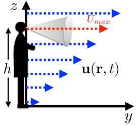
Figure 1: Schematic of the problem studied. A person talking either normally (exit speed of droplets around $1m/s$) or strongly (exit speed of droplets around $5m/s$)Abkarian et al. (2020); Cummins et al. (2020), and under the presence of an external flow u(r,t).

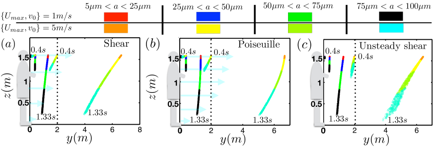
Figure 2: A person talking and spreading micrometric droplets of radius $a$ ranging from 5 $\mu m$ to 100 $\mu m$. The spreading is under the presence of an external flow u, and it is shown for three different times after the droplets were ejected from a cone shape of velocities modeling a person’s mouth namely, $t=0.08s,t=0.4s$, and $t=1.33s$. (a), Drops’ distribution during a normal and strong talk with exit speed of $v_{0}=1m/s$ and $v_{0}=5m/s$, respectively; and under a shear flow with $U_{max}=\{1m/s,5m/s\}$ (see color code). (b) The same as in (a) but under the presence of a Poiseuille flow. (c) The same as in (a) but under the presence of an unsteady shear flow. The safe distancing is indicated as a vertical dotted-black line. The light blue arrows represent the flow profile.

II Physical model

Let us analyze the motion of noninteracting spherical droplets of mass $m$, radius $a$, in an environment with air density $\rho_{a}$ and air viscosity $\mu_{a}$, under gravity $\mathbf{g}$, and subject to an external flow of the form $\mathbf{u}\left(\mathbf{r},t\right)$, with a characteristic speed $U_{max}$, where $\mathbf{r}(t)=(x,y,z)$ is the droplet’s position, here $t$ represents time. In this study we will be considering three flows namely shear, Pouiseuille, and unsteady shear flow. Droplets immersed in these profiles will have a characteristic speed $v(t)$ which decreases as the droplets fall due to gravity. With the latter physical quantities a Reynolds number ($\mathfrak{Re}$) can be defined as $\mathfrak{Re}=\rho_{a}(U_{max}-v)a/\mu_{a}$ which satisfies $\mathfrak{Re}<1$. Therefore, these droplets individual dynamics described by their translational velocity, $\mathbf{v}(t)=(v_{x},v_{y},v_{z})$, follows the Maxey-Riley equationMaxey and Riley (1983)

$$m\frac{d\mathbf{v}}{dt} = \left(m-m_{a}\right)\mathbf{g+}m_{a}\left.\frac{D\mathbf{u}}{Dt}\right|_{\mathbf{r}}$$ (1)

$$-\frac{m_{a}}{2}\frac{d}{dt}\left(\mathbf{v}_{T}+\frac{a^{2}}{15}\left.\nabla^{2}\mathbf{u}\right|_{\mathbf{r}}\right)$$

$$-R_{T}\mathbf{v}_{T}-R_{T}a\frac{\mathbf{v}_{T}(0)}{\sqrt{\pi\upsilon_{a}t}}$$

$$-R_{T}a\int_{0}^{t}\frac{d\mathbf{v}_{T}}{d\tau}\frac{d\tau}{\sqrt{\pi\upsilon_{a}\left(t-\tau\right)}},$$

where $m_{a}$ is the mass of air displaced by the sphere, $\upsilon_{a}=\mu_{a}/\rho_{a}$ represents the kinematic viscosity, $R_{T}=6\pi a\mu_{a}$ is the resistance coefficient; while $\rho$ indicates the droplet’s density. In addition, the following definitions are included:

$$\mathbf{v}_{T} = \mathbf{v-}\left.\mathbf{u}\right|_{\mathbf{r}}-\frac{a^{2}}{6}\left.\nabla^{2}\mathbf{u}\right|_{\mathbf{r}}$$ (2)

$$\frac{D\mathbf{u}}{Dt} = \frac{\partial\mathbf{u}}{\partial t}+\mathbf{u\cdot\nabla u,}$$ (3)

$$\frac{d\mathbf{u}}{dt} = \frac{\partial\mathbf{u}}{\partial t}+\mathbf{v\cdot\nabla u.}$$ (4)

The forces on the right hand side of  Eq. (1) are respectively, the droplet’s weight; bouyancy force; forces in the undisturbed flow due to local pressure gradients; the added or virtual mass force; Stokes drag force; and the last two terms represent the Boussinesq-Basset memory force. To find the order-of-magnitude of each term in the Maxey-Riley Eq. (1), one can introduce the following dimensionless quantities $\overline{\mathbf{r}}=\mathbf{r}/a,\overline{\mathbf{v}}=\mathbf{v/}U,\overline{t}=\left(U/a\right)t,$ where the characteristic speed is defined as $U=mg/R_{T},$ which is the terminal velocity of a falling droplet. After applying those dimensionless variables to Eq. (1), one arrives at

$$Re\frac{d\overline{\mathbf{v}}}{d\overline{t}} = -\frac{9\lambda}{2}\left(1-\lambda\right)\mathbf{k+}\lambda Re\left.\frac{D\overline{\mathbf{u}}}{D\overline{t}}\right|_{\overline{\mathbf{r}}}$$ (5)

$$-\frac{\lambda Re}{2}\frac{d}{d\overline{t}}\left(\overline{\mathbf{v}}_{T}\mathbf{+}\frac{1}{15}\left.\overline{\nabla}^{2}\overline{\mathbf{u}}\right|_{\overline{\mathbf{r}}}\right)$$

$$-\frac{9\lambda}{2}\overline{\mathbf{v}}_{T}-\frac{9\lambda\sqrt{Re}}{2\sqrt{\pi}}\frac{\overline{\mathbf{v}}_{T}(0)}{\sqrt{\overline{t}}}$$

$$-\frac{9\lambda\sqrt{Re}}{2\sqrt{\pi}}\int_{0}^{\overline{t}}\frac{d\overline{\mathbf{v}}_{T}}{d\overline{\tau}}\frac{d\overline{\tau}}{\sqrt{\left(\overline{t}-\overline{\tau}\right)}}.$$

where the Reynolds number $Re=\rho_{a}Ua/\mu_{a}$ has been introduced, as well as the ratio $\lambda=m_{a}/m=\rho_{a}/\rho=1.225\times 10^{-3}$. Here $\overline{\mathbf{g}}=\mathbf{g}a/U^{2}$.

III Dynamics without Boussinesq-Basset memory

Let us start analyzing the order of magnitude estimate of the terms in Eq. (1) based on typical droplets ejected after talking. According to recent studiesAbkarian et al. (2020); Cummins et al. (2020); Fontes et al. (2020), the radius of those droplets range between $5\mu m$ to $100\mu m$, hence Table 1 shows their respective Reynolds number and the order-of-magnitude involved in Eq. (5).

Table 1: Order-of-magnitude for different terms appearing in the M-R Eq. (5) as a function of the radius $a$.

$a(\mu m)$	$Re$	$\lambda\sqrt{Re}$	$\lambda Re$
5	$8.4\times 10^{-4}$	$3.5\times 10^{-5}$	$1\times 10^{-6}$
10	0.0067	$1\times 10^{-4}$	$8.2\times 10^{-6}$
20	0.05	$2.83\times 10^{-4}$	$6.55\times 10^{-5}$
30	0.18	$5.2\times 10^{-4}$	$2.2\times 10^{-4}$
50	0.83	0.0011	0.001
100	6.7	0.0032	0.0082

From this table and for droplets of radius $a\in\left[5\mu m,20\mu m\right]$, the limit $Re\rightarrow 0$ can be applied to the M-R Eq. (5) to finally get

$$\overline{\mathbf{v}}_{T}=-\mathbf{k},$$ (6)

which  implies that the dynamics of droplets of this size is

$$\overline{v}_{x}=0;\overline{v}_{y}=\overline{u}_{y},\overline{v}_{z}=-1.$$ (7)

The latter result belongs to the so-called overdamped approximation, where inertia does not play a role, and particles immediately reach the external flow speed. Alternatively, by keeping inertia and neglecting terms of order $\sqrt{Re}$ and higher, the Maxey-Riley equation can be rewritten as

$$\frac{d\overline{\mathbf{v}}}{d\overline{t}}=-\overline{g}\left(\mathbf{k}+\overline{\mathbf{v}}_{T}\right).$$ (8)

This equation allows us to observe the dynamics of droplets at short times.

III.1 Shear and Poiseuille flows as external wind

Let us solve Eq. (8) under the presence of shear and Poiseuille flows modeling the effect of wind on the spherical droplets. These profiles are given by

$$\mathbf{u}=\left(U_{\max}\frac{z}{h}+U_{0}z\left(z-h\right)\right)\;\mathbf{j.}$$ (9)

Notice that the shear flow profile correspond to the case $U_{0}=0.$ Given Eq. (9), we solve Eq. (8) whose solution including dimensions and subject to $\mathbf{r}(0)=(0,0,h)$ and $\mathbf{v}(0)=(v_{x0},v_{y0},v_{z0})$ can be shown to be

$$v_{x}(t) = v_{x0}e^{-Kt},\text{ \ }v_{z}(t)=\gamma_{z}e^{-Kt}-\frac{g}{K},$$ (10)

$$v_{y}(t) = \gamma_{y}e^{-Kt}-U_{0}\left(\frac{\gamma_{z}}{K}\right)^{2}e^{-2Kt}+U_{0}\frac{\gamma_{z}g}{K}t^{2}e^{-Kt}$$ (11)

$$-Ate^{-Kt}+B-Ct+U_{0}\frac{g^{2}}{K^{2}}t^{2},$$

Figure 3: (a)-(c) Maximum dispersion ($y_{M}$) along the $y-$direction of spherical droplets as a function of the radius $a$, as well as a function of different external flows namely, shear, Poiseuille, and unsteady shear flow. The color code in (b) is valid for all figures. (a) Maximum dispersion for $a$ ranging from 5$\mu m$ to 10$\mu m$. (b) Maximum dispersion for $a$ ranging from 12$\mu m$ to 60$\mu m$. (c) Maximum dispersion for $a$ ranging from 60$\mu m$ to 100$\mu m$. (d)-(f) Flying time ($t_{F}$) of spherical droplets as a function of the radius $a$. Here, $v_{z}(0)=0$. Red circles represent the whole $z-$component in Eq. (LABEL:xz), while the black-solid line represents the approximated equation $t_{F}\approx{9\mu_{a}h}/{2\rho ga^{2}}$. (d) $a$ ranging from 5$\mu m$ to 20$\mu m$. (f) $a$ ranging from 20$\mu m$ to 60$\mu m$. (e) $a$ ranging from 60$\mu m$ to 100$\mu m$.

where $K=R_{T}/m$ and $\beta=K{a^{2}}U_{0}/3$. Integrating the velocities, we get

$$x(t) = -\frac{v_{x0}}{K}e^{-Kt}+s_{x},\text{ \ }z(t)=-\frac{\gamma_{z}}{K}e^{-Kt}-\frac{g}{K}t+s_{z},$$

$$y(t) = \frac{1}{K}\left(\frac{A}{K}-\gamma_{y}-\frac{2U_{0}\gamma_{z}g}{K^{3}}\right)e^{-Kt}$$ (13)

$$+\frac{1}{K}\left(A-\frac{2U_{0}\gamma_{z}g}{K^{2}}\right)te^{-Kt}-\frac{U_{0}\gamma_{z}g}{K^{2}}t^{2}e^{-Kt}$$

$$+\frac{U_{0}\gamma_{z}^{2}}{2K^{3}}e^{-2Kt}+s_{y}+Bt-\frac{C}{2}t^{2}+\frac{U_{0}g^{2}}{3K^{2}}t^{3},$$

where constants $A,B,C,\gamma_{y},\gamma_{z},s_{x},s_{y},s_{z}$ are defined in Appendix IX.

III.2 Unsteady shear flow as external wind

A more realistic situation, is to consider the fact that air flows for a while, and then stops, and then flows again. The simplest model is to assume a time-dependent shear flow scenario. This unsteady vector flow field $\mathbf{u}(\mathbf{r},t)$ should satisfy the time-dependent Navier-Stokes equations, which after assuming $\mathbf{u}(\mathbf{r},t)=(0,u_{y}\left(z,t\right),0)$, incompressibility, and a null pressure, reduce to

$$\frac{\partial u_{y}}{\partial t}=\upsilon_{a}\frac{\partial^{2}u_{y}}{\partial z^{2}}\mathbf{.}$$ (14)

This parabolic equation must satisfy $u_{y}\left(z,0\right)=\left(U_{\max}/h\right)z,u_{y}\left(0,t\right)=0,$ and $u_{y}\left(h,t\right)=U_{\max}/2\left(1+\cos\omega t\right)$. Its solution can be veryfied to be

$$u_{y}\left(z,t\right)=\sum_{m=1}^{\infty}D_{m}g(t)\sin\frac{m\pi z}{h}+\frac{U_{\max}}{2h}\left(1+\cos\omega t\right)z,$$ (15)

where

$$g(t) = e^{-d_{m}t}+\frac{d_{m}}{\omega}\sin\omega t-\cos\omega t,$$ (16)

$$D_{m} = \frac{\omega f_{m}}{d_{m}^{2}+\omega^{2}},$$ (17)

$$f_{m} = \left(-1\right)^{m+1}\omega U_{\max}/m\pi,$$ (18)

$$d_{m} = \upsilon_{a}\left(\frac{m\pi}{h}\right)^{2}.$$ (19)

Once Eq. (15) is available, it is plugged into Eq. (8) and its solution subject to $\mathbf{r}(0)=(0,0,h)$ and $\mathbf{v}(0)=(v_{x0},v_{y0},v_{z0})$ although very lengthy, can be analytically found. The dominant terms of the solution along the $y-$component for long times read

Figure 4: (a)-(c) Effect of higher order terms on the dispersion along the $y-$direction of spherical droplets as a function of radius $a$ and an external flow. Here $\Delta y=y_{MB}-y_{M}$, where $y_{MB}$ is the maximum travelled distance by a droplet along the $y$-direction containing first order terms ($a\leq 20\mu m$) or the full terms in the M-R equation ($a>20\mu m$), whereas $y_{M}$ represents the solution directly obtained from Eqs. (LABEL:xz) and (13). (d) Effect of higher order terms on the flying time of spherical droplets as a function of radius $a$. Here $\Delta t_{F}=t_{FB}-t_{F}$, where $t_{FB}$ is the flying time by a droplet containing first order terms ($a\leq 20\mu m$) or the full terms in the M-R equation ($a>20\mu m$); whereas $t_{F}$ represents the the solution directly obtained from Eqs. (LABEL:xz). (e)-(f) Linear convergence of $\Delta y=y_{MB}-y_{M}$ as the time-step in the simulations decreases. (e) Convergence for a droplet of radius $30\mu m$ after discretizing the full M-R equation (5). (f) Convergence for a droplet of radius $19\mu m$ after discretizing the overdamped M-R equation (22).

$$v_{y}(t) = -\frac{U_{\max}g}{2hK}t-\frac{U_{\max}g\left[K\cos(\omega t)+\omega\sin(\omega t)\right]}{2h(K^{2}+\omega^{2})}t,$$

$$y(t) = \frac{U_{\max}}{2h}\left\{\frac{g}{K^{2}}t-\frac{g}{2K}t^{2}\right.$$ (21)

$$\left.-\frac{g}{(K^{2}+\omega^{2})}\left[\frac{K}{\omega}t\sin(\omega t)-t\cos(\omega t)\right]\right\}.$$

Once Eq. (LABEL:xz), Eq. (13), and Eq. (21) are available, we can now exemplify a typical droplets’ dispersion (cloud) after a person talks and generates micrometric droplets (radius between 5 $\mu m$ to 100 $\mu m$ Abkarian et al. (2020); Cummins et al. (2020)), which are subject to either a shear flow (Fig. 3(a)), a Pouiseuille flow (Fig. 3(b)), or an unsteady shear flow (Fig. 3(c)). We simulate the situation of a normal and a strong talk by imposing an exit speed of droplets (from a cone shape of velocities representing a person’s mouth) of $v_{0}=1m/s$ and $v_{0}=5m/s$, respectively. The cloud is made of $1000$ droplets of random size between 5 $\mu m$ to 100 $\mu m$. Additionally, we impose a moderate ($U_{max}=5m/s$) and a calm ($U_{max}=1m/s$) wind scenario. The cone shape as the initial velocity distribution, and as observed from experimentsCummins et al. (2020), is implemented by imposing $\mathbf{v}(0)=(v_{0}\cos\varphi_{0}\sin\theta_{0},v_{0}\sin\varphi_{0}\sin\theta_{0},v_{0}\cos\theta_{0})$, whose angular polar and azimuthal initial extremum are set to $\theta_{0}^{max}=110^{o}$, $\theta_{0}^{min}=81^{o}$, $\varphi_{0}^{max}=110^{o}$, and $\varphi_{0}^{min}=81^{o}$. The case of a Poiseuille flow profile considers for a calm flow $\{U_{max},U_{0}\}=\{1m/s,-0.4m^{-1}s^{-1}\}$ wheread for a moderate flow $\{U_{max},U_{0}\}=\{5m/s,-2m^{-1}s^{-1}\}$: The simulations for the unsteady flow profile consider $\omega=0.5s^{-1}$. Finally, $(\varphi,\theta)$ will randomly vary between their extremum. The results can be visualized in Fig. 3 which shows the distribution of droplets at three different times namely, $t=0.08s$, $t=0.4s$, and $t=1.33s$. A color code indicating the droplets’ sizes is also introduced. The safe distancing is indicated as a vertical dotted-black line. Clearly, droplets move beyond the safe distancing. As it can be seen, droplets under a moderate wind and after only $1.33s$, are already $6m$ away from the person’s mouth. Droplets under a calm wind and less than $50\mu m$ in radius will overpass the safe distancing in the next second. These results indicate a potential danger for people in a public space since the safe distancing has been easily surpassed. We finally take Eq. (LABEL:xz), Eq. (13), and Eq. (21) to find the maximum travelled distance ($y_{M}$) along the $y-$direction as a function of droplets’ size, as well as a function of different external flows namely, shear, Poiseuille, and unsteady shear flow. The results are shown in Fig. Figs. 3(a)-(c). Figures 3(a)-(c) show that droplets under a Pouiseuille profile reached the the longest distance compared to the other analyzed profiles. This figure also indicates that for $U_{max}=5m/s$, droplets of radius $5\mu m$, and under a Poiseuille flow, can travel until $2000m$, while around $1500m$ under a shear flow. As expected, the condition of having a wind blowing and ceasing (unsteady flow) reduces the droplets maximum dispersion to around $750m$ for $U_{max}=5m/s$. On the other hand, our results to leading order indicate that the maximum travelled distance for small droplets ($5\mu m$ radius) under a shear/Poiseuille external flow with a maximum speed of $U_{max}=1m/s$ may easily reach more than 250 meters. The long distance achieved by these small droplets is because they remain in the air for around 600 seconds, see Figs. 3(d)-(e). In these figures, the flying time obtained from Eq. (LABEL:xz), is shown as a solid-black line; while the red circles represent the approximated equation $t_{F}\approx{9\mu_{a}h}/{2\rho ga^{2}}$. These figures also indicate that the largest ($100\mu m$ radius) droplets can only stay in the air for about $1.5s$. It is worth mentioning that all the studied droplets ($a\in\left[5\mu m,100\mu m\right]$) reached a constant vertical terminal velocity $U\approx mg/R_{T}$.

IV Dynamics with Boussinesq-Basset memory

In the literature, the Boussinesq-Basset (B-B) memory force has been less frequently considered, probably because of its order-of-magnitude and because of the required computational effort. However, there exist some theoreticalPrasath, Vasan, and Govindarajan (2019); Langlois, Farazmand, and Haller (2015); Maxey and Riley (1983); Guseva and andand Tamás Tél (2013); Haller (2019); Tatom (1988), numericalvan Hinsberg, ten Thije Boonkkamp, and Clercx (2011); Alexander (2004); Daitche and Tél (2014, 2011) and experimentalCandelier, Angilella, and Souhar (2004); Mordant and Pinton (2000) works dealing with this force. In this section we analyze the effect of the memory force term on the dispersion an flying time of spherical droplets.

Consider first small droplets ranging between $a\in\left[5\mu m,20\mu m\right]$. According to Table 1, their motion can be modeled by the M-R equation under the overdamped approximation. However, by keeping terms of order $\sqrt{Re}$ to see the effect of the B-B memory force, Eq. (5) reads

$$\overline{\mathbf{v}}_{T}=-\left(1-\lambda\right)\mathbf{k}-\sqrt{\frac{Re}{\pi}}\int_{0}^{\overline{t}}\frac{d\overline{\mathbf{v}}_{T}}{d\overline{\tau}}\frac{d\overline{\tau}}{\sqrt{\left(\overline{t}-\overline{\tau}\right)}}.$$ (22)

To solve this integro-differential equation, a first order Euler method is chosen. Under this method, a component of the B-B force term can be shown to be:

$$\int_{0}^{\overline{t}}\frac{d\overline{v}}{d\overline{\tau}}\frac{d\overline{\tau}}{\sqrt{\left(\overline{t}-\overline{\tau}\right)}}=\sum\limits_{i=1}^{k-1}\frac{\overline{v}_{i+1}-\overline{v}_{i}}{\sqrt{\Delta\overline{t}}}\alpha\left(k,i\right),$$ (23)

where we have assumed that $\Delta\overline{t}=\Delta\tau$ and defined $\alpha\left(k,i\right)=2\sqrt{k-i}-2\sqrt{k-1-i}$. After certain steps, one can prove that the overdamped M-R Eq. (22), along the $z-$direction and in dimensional variables, acquires the following discrete form for $k=3,...N$:

$$v_{z,k} = -\sqrt{\Delta t}\frac{c_{0}}{c_{1}}+\frac{c_{2}}{c_{1}}v_{z,k-1}$$ (24)

$$-\frac{c_{3}}{c_{1}}\sum\limits_{i=1}^{k-2}\left(v_{z,i+1}-v_{z,i}\right)\alpha\left(k,i\right),$$

Figure 5: Effect of the Boussinesq-Basset memory force term on the sedimentation velocity ($v_{z}(0)=0$), for two spherical droplets reaching their terminal velocity $U$. The black-solid lines indicate an exponential decay towards $U$ when the B-B term is absent. The red-dashed lines indicate a $t^{-1/2}$ decay when the B-B term is present.

where constants $c_{0},c_{1},c_{2},c_{3}$ are defined in Appendix X. A similar expression as Eq. (24) is obtained for the other spatial components. In the case of larger droplets and from Table 1, one notices that the order-of-magnitude of all terms in Eq. (5) is the same. Therefore, one has to solve for the full M-R Eq. (5). Using the Euler method together with Eq. (23), one can show that the discretized $z-$component of Eq. (5) in dimensional variables reads

$$v_{z,k} = -\frac{\Delta t}{b_{1}}Rg+\frac{b_{2}}{b_{1}}v_{z,k-1}$$ (25)

$$-\frac{b_{3}}{b_{1}}\sum\limits_{i=1}^{k-2}\left(v_{z,i+1}-v_{z,i}\right)\alpha\left(k,i\right),$$

where constants $R,b_{0},b_{1},b_{2},b_{3}$ are defined in Appendix X. The discretization of the other components in Eq. (5) is similar to Eq. (25). After posing Eq. (24) and Eq.(25), we are ready to find the droplets’ dynamics under higher order terms.

Because of the external flows we have chosen and from the simulations in Sec. III, we observe that the dynamics mostly occurs along the $z-y$ plane, and that initial conditions are not relevant for long times (at least for $\mathbf{v}_{T}(0)=0$); thus from now on, a 2D problem with initial conditions $v_{z}(0)=0$ and $v_{y}(0)=U_{max}$, will be considered. Equations (5) and (22) are then numerically solved using the discretized scheme in Eq. (24) and Eq. (25), under the presence of a shear flow (the other flows basically share the same features), and for two typical exit initial speeds while talking Abkarian et al. (2020); Cummins et al. (2020) namely, $1m/s$ and $5m/s$. The time-step used for solving Eq. (5) and Eq. (22) was $4\times 10^{-4}s$ and $5\times 10^{-3}s$, respectively. The results of the simulations are shown in Figs. 4(a)-(c). In those figures, $\Delta y=y_{MB}-y_{M}$, where $y_{MB}$ is the maximum travelled distance along the $y$-direction by droplets of size $a\leq 20\mu m$ and obtained from Eq. (22). For droplets of size $a>20\mu m$, $y_{MB}$ represents the maximum travelled distance along the $y$-direction obtained after solving the full M-R equation (5); whereas $y_{M}$ represents the solution directly obtained from Eqs. (LABEL:xz) and (13). One can observe that for a low wind speed, the effect of higher order terms barely enhance the droplets’ dispersion. However, for a wind speed of $5m/s$ and for the smallest considered droplet, higher order terms can increase its dispersion around 2 $m$. Figures 4(a)-(c) also indicate that as the size of the droplets increases, higher order terms effects become smaller until they finally disappear.

The effect of first order terms and the full terms in the M-R equation, on the flying time of spherical droplets as a function of the radius $a$ is also analyzed. Using Eq. (LABEL:xz), the numerical solutions from Eq. (24) and Eq. (25), and defining $\Delta t_{F}=t_{FB}-t_{F}$; where for $a\leq 20\mu m$, $t_{FB}$ represents the flying time of a droplet calculated using first order terms (Eq. (22)). For $a>20\mu m$, $t_{FB}$ represents the flying time calculated using the full terms in the M-R equation. On the other hand, $t_{F}$ is the flying time directly obtained from Eqs. (LABEL:xz). This analysis is shown in Fig. 3(d). It can be seen that $\Delta t_{F}$ increases as the droplets’ sizes decrease. In fact, for $a=5\mu m$ there is a $0.8s$ flying time difference between the dynamics of Eq. (5) and Eq. (8). This extra time also contributes to the observed enhancement of dispersion of small droplets. A numerical analysis on the convergence of $\Delta y=y_{MB}-y_{M}$, as the time-step $\Delta t$ in the simulations decreases, is also performed. Fig. 4(f) shows this convergence for a droplet of radius $30\mu m$ after discretizing the full M-R equation (5). As expected, a linear convergence can be appreciated. The convergence for a droplet of radius $19\mu m$ and after using the overdamped M-R equation (22) is shown in Fig. 3(b). Once again a linear convergence is achieved. Therefore, the latter analysis validates our employed first order numerical algorithm.

Finally, the implications of the Boussinesq-Basset memory force term on the sedimentation velocity component $v_{z}(t)$ with $v_{z}(0)=0$ is also studied. The numerical results are shown in Fig. 5, which illustrates the dynamics of $v_{z}(t)+U$ versus time in a log-log plot, and for two different spherical droplets reaching their terminal velocity $U$. The black-solid lines belong to an exponential decay of $v_{z}(t)$ towards $U$; whereas the red-dashed lines indicate a $t^{-1/2}$ decay. It can be observed that for short times, $v_{z}(t)$ exponentially decays towards $U$; however, $v_{z}(t)$ decays according to the scaling $t^{-1/2}$ for long times. This is a rather surprising result, since the order-of-magnitude of the B-B term is really small. This $t^{-1/2}$ decay of the sedimenting velocity has been also recently reportedPrasath, Vasan, and Govindarajan (2019). Further consequences of the B-B term on the motion of particles at low Reynolds numbers may be search for in future investigations.

Figure 6: (a) Droplets’ distribution at $t=5s$ under a shear (S) and an unsteady shear flow (UNS) at calm ($1m/s$) and moderate winds ($5m/s$). The rest of the parameters are the same as in Fig. 2. Under these parameters, together with $RH=50\%$ and temperature les than $30^{o}C$, evaporation does not play a roleDbouk and Drikakis (2020). (b) Comparison of droplets’ position under an uniform flow ($\{h,U_{max},v_{0}\}=\{h=1.7m,1.1m/s,1m/s\}$) either using single particle dynamics (this work), or using a more elaborated CFD analysisDbouk and Drikakis (2020). (c) Droplets’ distribution at $t=\{1s,2s,3s,4s,5s\}$, and linear paths followed by some droplets of different sizes under an uniform flow. See Fig. 2 for color code.

V Discussions and conclusions

According to Dbouk and DrikakisDbouk and Drikakis (2020) and others, evaporation and relative humidity play a role on droplets’ dispersion. Those factors may reduce or increase the size of droplets and their cloud shape as it travels. Therefore, our results could be improved to account for a rocket-like dynamics (drops varying mass). Following Dbouk and DrikakisDbouk and Drikakis (2020), who considered a conjugated flow-heat-mass transfer problem and CFD dynamics, it can be conclued that evaporation of droplets takes place at high relative humidities, and high temperatures. Thus for the case of countries with an annual average of relative humidity, $RH=50\%$, a wind speed of $4km/h=1.1m/s$, a temperature less than $30C^{o}$, and five seconds later since a cloud of droplets originated, there will be a null evaporationDbouk and Drikakis (2020). Other works also supporting a long time survival of infected droplets is Stadnytskyi et al.Stadnytskyi et al. (2020)

Based on this information, Fig. 6(a) shows four droplets’ distributions (cloud) five seconds later since the cloud originated under a shear ($S$) or an unsteady shear ($UNS$) flow with $\{U_{max},v_{0}\}=\{1m/s,5m/s\}$. The other numerical parameters employed and the initial velocity distribution of droplets are the same as in Fig. 2. This figure indicates that droplets with $a>75\mu m$ have already reached the floor, and that droplets of size $50\mu m<a<75\mu m$ are about to reach the floor. However, the smallest droplets under a calm wind ($1m/s$) for both $UNS$ and $S$, have surpassed the social distancing (vertical black-dashed lines). The same droplets under a moderate wind ($5m/s$) for both $UNS$ and $S$, reached $15m$ and $25m$, respectively. Thus from this figure, one can explicitly visualize a more real scale to which people may be in risk of contagion. Fig. 6(b) compares the position of droplets’ distribution (cloud) under an uniform flow ($\{h,U_{max},v_{0}\}=\{h=1.7m,1.1m/s,1m/s\}$), either using single particle dynamics (this work) or employing a more elaborated CFD analysisDbouk and Drikakis (2020). Both methods result in a similar cloud’s position. Finally, using the latter parameters, the droplets’ distribution at $t=\{1s,2s,3s,4s,5s\}$ and some paths followed by droplets of different sizes are shown in Fig.6(c). These paths have a linear behavior since the cloud dynamics is practically overdamped, implying $y(t)\approx U_{max}t$ and $z(t)\approx h-Ut$, thus particles will follow the function $z\approx h-(U/U_{max})y$.

In summary, using single particle dynamics, which has the advantage of requiring a minimum computational cost, this paper provided an estimate of the maximum dispersion of micrometric droplets generated after talking. Briefly, under conditions of a null evaporation and only five seconds later since droplets were originated, it was found that an unsteady shear calm wind ($1m/s$) can disperse droplets beyond the social distancing, and until more than $15m$ when droplets are subject to a moderate unsteady shear flow ($5m/s$). As expected, an unsteady shear profile is less efficient to disperse droplets than a constant Poiseuille or shear profile. These constants profiles modeling a calm wind ($1m/s$) were found to provide a maximum dispersion beyond $250m$ for the smallest droples ($5\mu m$). The effect of the Boussinesq–Basset force term was also analyzed. Although its order-of magnitude is small, it was found to be enough to change the behavior of the sedimentation velocity (from exponentially decaying towards its terminal velocity, to proportionally decaying as $t^{-1/2}$) of a micrometric particle and slightly increase droplets’ dispersion and their flying time.

Future research would be to consider external flows in the presence of buildings and to find the complex streamlines generated and their effects on droplets’ distribution. It may be inferred for example that the presence of a corner on a common street, could generate stagnation points, that may risk areas of infection, since those points could storage for a while infected droplets. Furthermore, walls may induce three-dimensional flows that may drag particles away from the floor, thus increasing its flying time and hence their capability of traveling longer. We hope this study helps people to be more aware about the effect of daily wind currents on the propagation of potentially infected droplets. Based on our findings of droplets easily dispersing beyond the social distancing when subject to wind currents, we recommend the use of masksBhagat et al. (2020) able to contain the virus, as well as flex seal googles, since droplets dragged by wind may reach eyes. We also recommend to wash all your wearing clothes and shoes, and to shower after being out from home, since infected droplets may be attached to clothes or hairFeng et al. (2020). Direct exposure to wind currents, mainly in crowded cities, should also be avoided.

VI Author contributios

All authors contributed equally to this research.

VII Acknowledgements

M. S. thanks Consejo Nacional de Ciencia y Tecnologia, CONACyT for support. M. S. dedicates this paper to the memory of his relatives Arturo Sandoval and Marcos Fernandez reached by this pandemic.

VIII Data availability

The data that support the findings of this study are available from the corresponding author upon reasonable request.

IX Appendix 1: Constants added

The constants $A,B,C,\gamma_{y},\gamma_{z},s_{x},s_{y},s_{z}$ appearing in Eqs. (10)-(13) are defined as

$$A = \gamma_{z}\left(\frac{U_{\max}}{h}+U_{0}\left(2s_{z}-h\right)\right),$$ (26)

$$B = U_{0}s_{z}^{2}+\frac{\beta}{K}$$ (27)

$$+\left(U_{0}\left[\frac{2g}{K^{2}}-h\right]+\frac{U_{\max}}{h}\right)\left(\frac{g}{K^{2}}+s_{z}\right),$$

$$C = \frac{g}{K}\left[U_{0}\left(2\left(\frac{g}{K^{2}}+s_{z}\right)-h\right)+\frac{U_{\max}}{h}\right],$$ (28)

$$\gamma_{y} = v_{y0}+U_{0}\left(\left(\frac{\gamma_{z}}{K}\right)^{2}-s_{z}^{2}\right)$$

$$-\left(U_{0}\left(\frac{2g}{K^{2}}-h\right)+\frac{U_{\max}}{h}\right)\left(\frac{g}{K^{2}}+s_{z}\right)-\frac{\beta}{K},$$

$$\gamma_{z} = v_{z0}+\frac{g}{K},s_{x}=\frac{v_{x0}}{K},s_{z}=h+\frac{\gamma_{z}}{K},$$ (30)

$$s_{y} = -\frac{1}{K}\left[\frac{A}{K}-\gamma_{y}+\frac{U_{0}\gamma_{z}}{K^{2}}\left(\frac{\gamma_{z}}{2}-\frac{2g}{K}\right)\right].$$ (31)

X Appendix 2: Numerical part for the B-B equation

The constants $c_{0},c_{1},c_{2},c_{3}$ appearing in Eq. (24) are defined as

$$c_{0} = \frac{g\left(m-m_{a}\right)}{R_{T}},$$ (32)

$$c_{1} = \frac{2a}{\sqrt{\pi\upsilon_{a}}}+\sqrt{\Delta t},$$ (33)

$$c_{2} = \frac{2a}{\sqrt{\pi\upsilon_{a}}},c_{3}=\frac{c_{2}}{2},$$ (34)

whereas constants $R,b_{1},b_{2},b_{3}$ appearing in Eq. (25) are

$$R = (1-\lambda)/D\text{ with }D=1+\lambda/2,$$ (35)

$$b_{1} = \left(1+\sqrt{\Delta t}\frac{2Ka}{D\sqrt{\pi\upsilon_{a}}}\right),$$ (36)

$$b_{2} = \sqrt{\Delta t}\frac{2Ka}{D\sqrt{\pi\upsilon_{a}}}-\Delta t\frac{K}{D}+1,$$ (37)

$$b_{3} = \sqrt{\Delta t}\frac{Ka}{D\sqrt{\pi\upsilon_{a}}}.$$ (38)

References

- Zhang et al. (2020) R. Zhang, Y. Li, A. L. Zhang, Y. Wang, and M. J. Molina, “Identifying airborne transmission as the dominant route for the spread of covid-19,” Proceedings of the National Academy of Sciences 117, 14857–14863 (2020), https://www.pnas.org/content/117/26/14857.full.pdf .
- Mittal, Ni, and Seo (2020) R. Mittal, R. Ni, and J.-H. Seo, “The flow physics of covid-19,” Journal of Fluid Mechanics 894, F2 (2020).
- Abkarian and Stone (2020) M. Abkarian and H. A. Stone, “Stretching and break-up of saliva filaments during speech: A route for pathogen aerosolization and its potential mitigation,” Physical Review Fluids 5, 102301 (2020).
- Abkarian et al. (2020) M. Abkarian, S. Mendez, N. Xue, F. Yang, and H. A. Stone, “Speech can produce jet-like transport relevant to asymptomatic spreading of virus,” Proceedings of the National Academy of Sciences 117, 25237–25245 (2020), https://www.pnas.org/content/117/41/25237.full.pdf .
- Wright (2020) K. Wright, “How talking spreads viruses,” Physics 13, 195 (2020).
- Bourouiba (2020) L. Bourouiba, “Turbulent Gas Clouds and Respiratory Pathogen Emissions: Potential Implications for Reducing Transmission of COVID-19,” JAMA 323, 1837–1838 (2020).
- Jones et al. (2020) N. R. Jones, Z. U. Qureshi, R. J. Temple, J. P. J. Larwood, T. Greenhalgh, and L. Bourouiba, “Two metres or one: what is the evidence for physical distancing in covid-19?” BMJ 370 (2020), 10.1136/bmj.m3223, https://www.bmj.com/content/370/bmj.m3223.full.pdf .
- Bhagat et al. (2020) R. K. Bhagat, M. S. Davies Wykes, S. B. Dalziel, and P. F. Linden, “Effects of ventilation on the indoor spread of covid-19,” Journal of Fluid Mechanics 903, F1 (2020).
- Park et al. (2020) S. Park, Y. Kim, S. Yi, S. Lee, B. Na, C. Kim, and E. Jeong, “Coronavirus disease outbreak in call center, south korea,” Emerging Infectious Diseases 26(8), 1666–1670 ((2020)).
- Cummins et al. (2020) C. P. Cummins, O. J. Ajayi, F. V. Mehendale, R. Gabl, and I. M. Viola, “The dispersion of spherical droplets in source-sink flows and their relevance to the covid-19 pandemic,” Physics of Fluids 32, 083302 (2020).
- Dbouk and Drikakis (2020) T. Dbouk and D. Drikakis, “Weather impact on airborne coronavirus survival,” Physics of Fluids 32, 093312 (2020).
- (12) v. D. T. M. T. Blocken B, Malizia F, “Towards aerodynamically equivalent covid19 social distancing for walking and running. 2020,” Pre-print Available online: http://www.urbanphysics.net/COVID19AeroPaper.pdf. Accessed 26 Jan 2021 .
- Dhand and Li (2020) R. Dhand and J. Li, “Coughs and sneezes: their role in transmission of respiratory viral infections, including sars-cov-2,” American journal of respiratory and critical care medicine 202, 651–659 (2020).
- Feng et al. (2020) Y. Feng, T. Marchal, T. Sperry, and H. Yi, “Influence of wind and relative humidity on the social distancing effectiveness to prevent covid-19 airborne transmission: A numerical study,” Journal of aerosol science , 105585 (2020).
- Maxey and Riley (1983) M. R. Maxey and J. J. Riley, “Equation of motion for a small rigid sphere in a nonuniform flow,” The Physics of Fluids 26, 883–889 (1983).
- Fontes et al. (2020) D. Fontes, J. Reyes, K. Ahmed, and M. Kinzel, “A study of fluid dynamics and human physiology factors driving droplet dispersion from a human sneeze,” Physics of Fluids 32, 111904 (2020).
- Prasath, Vasan, and Govindarajan (2019) S. G. Prasath, V. Vasan, and R. Govindarajan, “Accurate solution method for the Maxey-Riley equation, and the effects of Basset history,” Journal of Fluid Mechanics 868, 428–460 (2019).
- Langlois, Farazmand, and Haller (2015) G. P. Langlois, M. Farazmand, and G. Haller, “Asymptotic dynamics of inertial particles with memory,” Journal of nonlinear science 25, 1225–1255 (2015).
- Guseva and andand Tamás Tél (2013) K. Guseva and U. F. andand Tamás Tél, “Influence of the history force on inertial particle advection: Gravitational effects and horizontal diffusion,” Physical Review E 88, 042909 (2013).
- Haller (2019) G. Haller, “Solving the inertial particle equation with memory,” Journal of Fluid Mechanics 874, 1–4 (2019).
- Tatom (1988) F. Tatom, “The basset term as a semiderivative,” Applied Scientific Research 45, 283–285 (1988).
- van Hinsberg, ten Thije Boonkkamp, and Clercx (2011) M. van Hinsberg, J. ten Thije Boonkkamp, and H. Clercx, “An efficient, second order method for the approximation of the basset history force,” Journal of Computational Physics 230, 1465 – 1478 (2011).
- Alexander (2004) P. Alexander, “High order computation of the history term in the equation of motion for a spherical particle in a fluid,” Journal of Scientific Computing 21, 129–143 (2004).
- Daitche and Tél (2014) A. Daitche and T. Tél, “Memory effects in chaotic advection of inertial particles,” New Journal of Physics 16, 073008 (2014).
- Daitche and Tél (2011) A. Daitche and T. Tél, “Memory effects are relevant for chaotic advection of inertial particles,” Physical review letters 107, 244501 (2011).
- Candelier, Angilella, and Souhar (2004) F. Candelier, J. R. Angilella, and M. Souhar, “On the effect of the boussinesq-basset force on the radial migration of a stokes particle in a vortex,” Physics of Fluids 16, 1765–1776 (2004).
- Mordant and Pinton (2000) N. Mordant and J.-F. Pinton, “Velocity measurement of a settling sphere,” The European Physical Journal B-Condensed Matter and Complex Systems 18, 343–352 (2000).
- Stadnytskyi et al. (2020) V. Stadnytskyi, C. E. Bax, A. Bax, and P. Anfinrud, “The airborne lifetime of small speech droplets and their potential importance in sars-cov-2 transmission,” Proceedings of the National Academy of Sciences 117, 11875–11877 (2020).