Tight Risk Bound for High Dimensional Time Series Completion

Abstract.

Initially designed for independent datas, low-rank matrix completion was successfully applied in many domains to the reconstruction of partially observed high-dimensional time series. However, there is a lack of theory to support the application of these methods to dependent datas. In this paper, we propose a general model for multivariate, partially observed time series. We show that the least-square method with a rank penalty leads to reconstruction error of the same order as for independent datas. Moreover, when the time series has some additional properties such as periodicity or smoothness, the rate can actually be faster than in the independent case.

1. Introduction

Low-rank matrix completion methods were studied in depth in the past 10 years. This was partly motivated by the popularity of the Netflix prize [9] in the machine learning community. The first theoretical papers on the topic covered matrix recovery from a few entries observed exactly [13, 14, 26]. The same problem was studied with noisy observations in [11, 12, 27, 23]. The minimax rate of estimation was derived by [30]. Since then, many estimators and many variants of this problem were studied in the statistical literature, see [42, 28, 32, 29, 38, 46, 18, 16, 4, 36, 37] for instance.
High-dimensional time series often have strong correlation, and it is thus natural to assume that the matrix that contains such a series is low-rank (exactly, or approximately). Many econometrics models are designed to generate series with such a structure. For example, the factor model studied in [31, 33, 34, 22, 17, 24] can be interpreted as a high-dimensional autoregressive (AR) process with a low-rank transition matrix. This model (and variants) was used and studied in signal processing [8] and statistics [42, 1]. Other papers focused on a simpler model where the series is represented by a deterministic low-rank trend matrix plus some possibly correlated noise. This model was used by [51] to perform prediction, and studied in [3].
It is thus tempting to use low-rank matrix completion algorithms to recover partially observed high-dimensional time series, and this was indeed done in many applications: [50, 48, 20] used low-rank matrix completion to reconstruct data from multiple sensors. Similar techniques were used by [40, 39] to recover the electricity consumption of many households from partial observations, by [5] on panel data in economics, and by [43, 7] for policy evaluation. Some algorithms were proposed to take into account the temporal updates of the observations (see [45]). However, it is important to note that 1) all the aforementioned theory on matrix completion, for example [30], was only developed for independent observations, and 2) most papers using these techniques on time series did not provide any theoretical justification that it can be used on dependent observations. One must however mention that [21] obtained theoretical results for univariate time series prediction by embedding the time series into a Hankel matrix and using low-rank matrix completion.
In this paper, we study low-rank matrix completion for partially observed high-dimensional time series that indeed exhibit a temporal dependence. We provide a risk bound for the reconstruction of a rank-$k$ matrix, and a model selection procedure for the case where the rank $k$ is unknown. Under the assumption that the univariate series are $\phi$-mixing, we prove that we can reconstruct the matrix with a similar error than in the i.i.d case in [30]. If, moreover, the time series has some additional properties, as the ones studied in [3] (periodicity or smoothness), the error can even be smaller than in the i.i.d case. This is confirmed by a short simulation study.
From a technical point of view, we start by a reduction of the matrix completion problem to a structured regression problem as in [38]. But on the contrary to [38], we have here dependent observations. We thus follow the technique of [2] to obtain risk bounds for dependent observations. In [2], it is shown that one can obtain risk bounds for dependent observations that are similar to the risk bounds for independent observations under a $\phi$-mixing assumption, using Samson’s version of Bernstein inequality [44]. For model selection, we follow the guidelines of [41]: we introduce a penalty proportional to the rank. Using the previous risk bounds, we show that this leads to an optimal rank selection.
The paper is organized as follows. In Section 2, we introduce our model, and the notations used throughout the paper. In Section 3, we provide the risk analysis when the rank $k$ is known. We then describe our rank selection procedure in Section 4 and show that it satisfies a sharp oracle inequality. The numerical experiments are in Section 5. All the proofs are gathered in Section 6.

Notations and basic definitions. Throughout the paper, $\mathcal{M}_{d,T}(\mathbb{R})$ is equipped with the Fröbénius scalar product

$$\langle.,.\rangle_{\mathcal{F}}:(\mathbf{A},\mathbf{B})\in\mathcal{M}_{d,T}(\mathbb{R})^{2}\longmapsto\textrm{trace}(\mathbf{A}^{*}\mathbf{B})=\sum_{j,t}\mathbf{A}_{j,t}\mathbf{B}_{j,t}$$

or with the spectral norm

$$\|.\|_{\textrm{op}}:\mathbf{A}\in\mathcal{M}_{d,T}(\mathbb{R})\longmapsto\sup_{\|x\|=1}\|\mathbf{A}x\|=\sigma_{1}(\mathbf{A}).$$

Let us finally remind the definition of the $\phi$-mixing condition on stochastic processes. Given two $\sigma$-algebras $\mathcal{A}$ and $\mathcal{B}$, we define the $\phi$-mixing coefficient between $\mathcal{A}$ and $\mathcal{B}$ by

$$\phi(\mathcal{A},\mathcal{B}):=\sup\left\{|\mathbb{P}(B)-\mathbb{P}(B|A)|\textrm{ $;$ }(A,B)\in\mathcal{A}\times\mathcal{B}\textrm{, }\mathbb{P}(A)\neq 0\right\}.$$

When $\mathcal{A}$ and $\mathcal{B}$ are independent, $\phi(\mathcal{A},\mathcal{B})=0$, more generally, this coefficient measure how dependent $\mathcal{A}$ and $\mathcal{B}$ are. Given a process $(Z_{t})_{t\in\mathbb{N}}$, we define its $\phi$-mixing coefficients by

$$\phi_{Z}(i):=\sup\left\{\phi(A,B)\textrm{ $;$ }t\in\mathbb{Z}\textrm{, }A\in\sigma(X_{h},h\leqslant t)\textrm{, }B\in\sigma(X_{\ell},\ell\geqslant t+i)\right\}.$$

Some properties and examples of applications of $\phi$-mixing coefficients can be found in [19].

2. Setting of the problem and notations

Consider $d,T\in\mathbb{N}^{*}$ and a $d\times T$ random matrix $\mathbf{M}$. Assume that the rows $\mathbf{M}_{1,.},\dots,\mathbf{M}_{d,.}$ are time series and that $Y_{1},\dots,Y_{n}$ are $n\in\{1,\dots,d\times T\}$ noisy entries of the matrix $\mathbf{M}$:

(1) $$Y_{i}=\textrm{trace}(\mathbf{X}_{i}^{*}\mathbf{M})+\xi_{i}\textrm{ $;$ }i\in\{1,\dots,n\},$$

where $\mathbf{X}_{1},\dots,\mathbf{X}_{n}$ are i.i.d random matrices distributed on

$$\mathcal{X}:=\{e_{\mathbb{R}^{d}}(j)e_{\mathbb{R}^{T}}(t)^{*}\textrm{ $;$ }1\leqslant j\leqslant d\textrm{ and }1\leqslant t\leqslant T\},$$

and $\xi_{1},\dots,\xi_{n}$ are i.i.d. centered random variables, with standard deviation $\sigma_{\xi}>0$, such that $\mathbf{X}_{i}$ and $\xi_{i}$ are independent for every $i\in\{1,\dots,n\}$. Note that, as $\mathbf{X}_{1},\dots,\mathbf{X}_{n}$ are independent, we do not exclude multiple observations of the same entry. That is, our model of matrix completion is the one studied in [30, 42, 38] rather than the model in [11, 12] where this is not possible.
Let us now describe the time series structure of each $\mathbf{M}_{1,.},\dots,\mathbf{M}_{d,.}$. We assume that each series $\mathbf{M}_{j,.}$ can be decomposed as a deterministic component $\mathbf{\Theta}^{0}_{j,.}$ plus some random noise $\varepsilon_{j,.}$. The noise can exhibit some temporal dependence: $\varepsilon_{j,t}$ will not be independent from $\varepsilon_{j,t^{\prime}}$ in general. Moreover, as discussed in [3], $\mathbf{\Theta}_{j,.}^{0}$ can have some more structure: $\mathbf{\Theta}_{j,.}^{0}=\mathbf{T}_{j,.}^{0}\mathbf{\Lambda}$ for some known matrix ${\bf\Lambda}$. Examples of such structures (smoothness or periodicity) are discussed below. This gives

(2) $$\left\{\begin{array}[]{rcl}\mathbf{M}&=&\mathbf{\Theta}^{0}+\varepsilon\\ \mathbf{\Theta}^{0}&=&\mathbf{T}^{0}\mathbf{\Lambda}\end{array}\right.,$$

where $\varepsilon$ is a $d\times T$ random matrix having i.i.d. and centered rows, $\mathbf{\Lambda}\in\mathcal{M}_{\tau,T}(\mathbb{C})$ ($\tau\leqslant T$) is known and $\mathbf{T}^{0}$ is an unknown element of $\mathcal{M}_{d,\tau}(\mathbb{R})$ such that

(3) $$\sup_{j,t}|\mathbf{T}_{j,t}^{0}|\leqslant\frac{\mathfrak{m}_{0}}{\mathfrak{m}_{\mathbf{\Lambda}}(\tau)}\textrm{ with }\mathfrak{m}_{0}>0\textrm{ and }1\vee\sup_{{\bf T}\in\mathcal{M}_{d,\tau}(\mathbb{R})}\left\{\frac{\sup_{j,t}|(\mathbf{T}\mathbf{\Lambda})_{j,t}|}{\sup_{j,\ell}|\mathbf{T}_{j,\ell}|}\right\}\leqslant\mathfrak{m}_{\mathbf{\Lambda}}(\tau)<\infty.$$

Note that this leads to

$$\sup_{j,t}|\mathbf{\Theta}_{j,t}^{0}|\leqslant\sup_{j,\ell}|\mathbf{T}_{j,\ell}^{0}|\cdot\frac{\sup_{j,t}|(\mathbf{T}^{0}\mathbf{\Lambda})_{j,t}|}{\sup_{j,\ell}|\mathbf{T}_{j,\ell}^{0}|}\leqslant\mathfrak{m}_{0}$$

and

$$\mathfrak{m}_{\bf\Lambda}:=\sup_{j,t}|\mathbf{\Lambda}_{j,t}|<\infty.$$

We now make the additional assumption that the deterministic component is low-rank, reflecting the strong correlation between the different series. Precisely, we assume that $\mathbf{T}^{0}$ is of rank $k\in\{1,\dots,d\wedge T\}$: $\mathbf{T}^{0}=\mathbf{U}^{0}\mathbf{V}^{0}$ with $\mathbf{U}^{0}\in\mathcal{M}_{d,k}(\mathbb{R})$ and $\mathbf{V}^{0}\in\mathcal{M}_{k,\tau}(\mathbb{R})$. The rows of the matrix $\mathbf{V}^{0}$ may be understood as latent factors. By Equations (1) and (2), for any $i\in\{1,\dots,n\}$,

(4) $$Y_{i}=\textrm{trace}(\mathbf{X}_{i}^{*}\mathbf{\Theta}^{0})+\overline{\xi}_{i}$$

with $\overline{\xi}_{i}:=\textrm{trace}(\mathbf{X}_{i}^{*}\varepsilon)+\xi_{i}$. It is reasonable to assume that $\mathbf{X}_{i}$ and $\xi_{i}$, which are random terms related to the observation instrument, are independent to $\varepsilon$, which is the stochastic component of the observed process. Then, since $\xi_{i}$ is a centered random variable and $\varepsilon$ is a centered random matrix,

$$\mathbb{E}(\overline{\xi}_{i})=\mathbb{E}(\langle\mathbf{X}_{i},\varepsilon\rangle_{\mathcal{F}})+\mathbb{E}(\xi_{i})=\sum_{j=1}^{d}\sum_{t=1}^{T}\mathbb{E}((\mathbf{X}_{i})_{j,t})\mathbb{E}(\varepsilon_{j,t})=0.$$

This legitimates to consider the following least-square estimator of the matrix $\mathbf{\Theta}^{0}$:

(5) $$\left\{\begin{array}[]{rcl}\widehat{\mathbf{\Theta}}_{k,\tau}&=&\widehat{\mathbf{T}}_{k,\tau}\mathbf{\Lambda}\\ \widehat{\mathbf{T}}_{k,\tau}&\in&\displaystyle{\arg\min_{\mathbf{T}\in\mathcal{S}_{k,\tau}}r_{n}(\mathbf{T}\mathbf{\Lambda})}\end{array}\right.,$$

where $\mathcal{S}_{k,\tau}$ is a subset of

$$\mathcal{M}_{d,k,\tau} := \left\{\mathbf{U}\mathbf{V}\textrm{ $;$ }(\mathbf{U},\mathbf{V})\in\mathcal{M}_{d,k}(\mathbb{R})\times\mathcal{M}_{k,\tau}(\mathbb{R})\textrm{ s.t. }\sup_{j,\ell}|\mathbf{U}_{j,\ell}|\leqslant\sqrt{\frac{\mathfrak{m}_{0}}{k\mathfrak{m}_{\mathbf{\Lambda}}(\tau)}}\right.$$

$$\hskip 256.0748pt\left.\textrm{ and }\sup_{\ell,t}|\mathbf{V}_{\ell,t}|\leqslant\sqrt{\frac{\mathfrak{m}_{0}}{k\mathfrak{m}_{\mathbf{\Lambda}}(\tau)}}\right\},$$

and

$$r_{n}(\mathbf{A}):=\frac{1}{n}\sum_{i=1}^{n}(Y_{i}-\langle\mathbf{X}_{i},\mathbf{A}\rangle_{\mathcal{F}})^{2}\textrm{ $;$ }\forall\mathbf{A}\in\mathcal{M}_{d,T}(\mathbb{R}).$$

Remark 2.1.

In many cases, we will simply take $\mathcal{S}_{k,\tau}=\mathcal{M}_{d,k,\tau}$. However, in many applications, it is natural to impose stronger constraints on the estimators. For example, in nonnegative matrix factorization, we would have

$$\mathcal{S}_{k,\tau}=\{\mathbf{U}\mathbf{V}\textrm{ $;$ }(\mathbf{U},\mathbf{V})\in\mathcal{M}_{d,k,\tau}\textrm{ s.t. }\forall j,\ell,t\textrm{, }\mathbf{U}_{j,\ell}\geqslant 0\textrm{ and }\mathbf{V}_{\ell,t}\geqslant 0\}$$

(see e.g. [40]). So for now, we only assume that $\mathcal{S}_{k,\tau}\subset\mathcal{M}_{d,k,\tau}$. Later, we will specify some sets $\mathcal{S}_{k,\tau}$.

Let us conclude this section with two examples of matrices $\mathbf{\Lambda}$ corresponding to usual time series structures. On the one hand, if the trend of the multivalued time series $\mathbf{M}$ is $\tau$-periodic, with $T\in\tau\mathbb{N}^{*}$, one can take $\mathbf{\Lambda}=(\mathbf{I}_{\tau}|\cdots|\mathbf{I}_{\tau})$, and then $\mathfrak{m}_{\bf\Lambda}=1$ and $\mathfrak{m}_{\bf\Lambda}(\tau):=1$ works. So, in this case, note that the usual matrix completion model of [30] is part of our framework by taking $T=\tau$. On the other hand, assume that for any $j\in\{1,\dots,d\}$, the trend of $\mathbf{M}_{j,.}$ is a sample on $\{0,1/T,2/T,\dots,1\}$ of a function $f_{j}:[0,1]\rightarrow\mathbb{R}$ belonging to a Hilbert space $\mathcal{H}$. In this case, if $(\mathbf{e}_{n})_{n\in\mathbb{Z}}$ is a Hilbert basis of $\mathcal{H}$, one can take $\mathbf{\Lambda}=(\mathbf{e}_{n}(t/T))_{|n|\leqslant N,1\leqslant t\leqslant T}$. For instance, if $f_{j}\in\mathbb{L}^{2}([0,1];\mathbb{R})$, a natural choice is the Fourier basis $\mathbf{e}_{n}(t)=e^{2i\pi nt/T}$, and then $\mathfrak{m}_{\bf\Lambda}=1$ and

$$\frac{\sup_{j,t}|(\mathbf{T}\mathbf{\Lambda})_{j,t}|}{\sup_{j,\ell}|\mathbf{T}_{j,\ell}|}\leqslant\frac{1}{\sup_{j,\ell}|\mathbf{T}_{j,\ell}|}\cdot\sup_{j,t}\sum_{\ell=1}^{\tau}|\mathbf{T}_{j,\ell}e^{2i\pi nt/T}|\leqslant\tau=:\mathfrak{m}_{\bf\Lambda}(\tau).$$

Here, the usual matrix completion model of [30] is not part of our framework because $T$ is possibly huge and to take $\tau=T$ implies that the coefficients of the matrix $\mathbf{T}^{0}$ are all unrealistically small by Condition (3). However, wathever the time series structure taken into account via $\mathbf{\Lambda}$, our model is designed for small values of $\tau$. Else, the model of [30] is appropriate. So, when $\mathbf{\Lambda}$ is the previous Fourier matrix, and in general when $\mathfrak{m}_{\bf\Lambda}(\tau)$ is a non constant increasing function of $\tau$, we assume that $\tau\in\llbracket 1,\tau_{0}\rrbracket$ with $\tau_{0}\ll T$.

3. Risk bound on $\widehat{\mathbf{T}}_{k,\tau}$

3.1. Upper bound

First of all, since $\mathbf{X}_{1},\dots,\mathbf{X}_{n}$ are i.i.d $\mathcal{X}$-valued random matrices, there exists a probability measure $\Pi$ on $\mathcal{X}$ such that

$$\mathbb{P}_{\mathbf{X}_{i}}=\Pi\textrm{ $;$ }\forall i\in\{1,\dots,n\}.$$

In addition to the two norms on $\mathcal{M}_{d,T}(\mathbb{R})$ introduced above, let us consider the scalar product $\langle.,.\rangle_{\mathcal{F},\Pi}$ defined on $\mathcal{M}_{d,T}(\mathbb{R})$ by

$$\langle\mathbf{A},\mathbf{B}\rangle_{\mathcal{F},\Pi}:=\int_{\mathcal{M}_{d,T}(\mathbb{R})}\langle X,\mathbf{A}\rangle_{\mathcal{F}}\langle X,\mathbf{B}\rangle_{\mathcal{F}}\Pi(dX)\textrm{ $;$ }\forall\mathbf{A},\mathbf{B}\in\mathcal{M}_{d,T}(\mathbb{R}).$$

Remarks:

1. For any deterministic $d\times T$ matrices $\mathbf{A}$ and $\mathbf{B}$,

   $$\langle\mathbf{A},\mathbf{B}\rangle_{\mathcal{F},\Pi}=\mathbb{E}(\langle\mathbf{A},\mathbf{B}\rangle_{n})$$

   where $\langle.,.\rangle_{n}$ is the empirical scalar product on $\mathcal{M}_{d,T}(\mathbb{R})$ defined by

   $$\langle\mathbf{A},\mathbf{B}\rangle_{n}:=\frac{1}{n}\sum_{i=1}^{n}\langle\mathbf{X}_{i},\mathbf{A}\rangle_{\mathcal{F}}\langle\mathbf{X}_{i},\mathbf{B}\rangle_{\mathcal{F}}.$$

   However, note that this relationship between $\langle.,.\rangle_{\mathcal{F},\Pi}$ and $\langle.,.\rangle_{n}$ doesn’t hold anymore when $\mathbf{A}$ and $\mathbf{B}$ are random matrices.

2. Note that if the sampling distribution $\Pi$ is uniform, then $\|.\|_{\mathcal{F},\Pi}^{2}=(dT)^{-1}\|.\|_{\mathcal{F}}^{2}$.

Notation. For every $i\in\{1,\dots,n\}$, let $\chi_{i}$ be the couple of coordinates of the nonzero element of $\mathbf{X}_{i}$, which is a $\mathcal{E}$-valued random variable with $\mathcal{E}=\{1,\dots,d\}\times\{1,\dots,T\}$.

In the sequel, $\varepsilon$, $\xi_{1},\dots,\xi_{n}$ and $\mathbf{X}_{1},\dots,\mathbf{X}_{n}$ fulfill the following additional conditions.

Assumption 3.1.

The rows of $\varepsilon$ are independent and identically distributed. There is a process $(\varepsilon_{t})_{t\in\mathbb{Z}}$ such that each $\varepsilon_{j,.}$ has the same distribution than $(\varepsilon_{1},\dots,\varepsilon_{T})$, and such that

$$\Phi_{\varepsilon}:=1+\sum_{i=1}^{n}\phi_{\varepsilon}(i)^{1/2}<\infty.$$

Assumption 3.2.

There exists a deterministic constant $\mathfrak{m}_{\varepsilon}>0$ such that

$$\sup_{j,t}|\varepsilon_{j,t}|\leqslant\mathfrak{m}_{\varepsilon}.$$

Moreover, there exist two deterministic constants $\mathfrak{c}_{\xi},\mathfrak{v}_{\xi}>0$ such that

$$\sup_{i\in\{1,\dots,n\}}\mathbb{E}(\xi_{i}^{2})\leqslant\mathfrak{v}_{\xi}$$

and, for every $q\geqslant 3$,

$$\sup_{i\in\{1,\dots,n\}}\mathbb{E}(|\xi_{i}|^{q})\leqslant\frac{\mathfrak{v}_{\xi}\mathfrak{c}_{\xi}^{q-2}q!}{2}.$$

This assumption means that the $\varepsilon_{j,t}$’s are bounded, and that the $\xi_{i}$’s are sub-exponential random variables. Sub-exponential random variables include bounded and Gaussian variables as special cases. Note that this is the assumption made on the noise for the matrix completion in the i.i.d. framework in the papers mentioned above [38, 30]. The boundedness of the $\varepsilon_{j,t}$’s can be seen as quite restrictive. However, we are not aware of any way to avoid this assumption in this setting. Indeed, it allows to apply Samson’s concentration inequality for $\phi$-mixing processes (see Samson [44]). In [2], the authors prove sharp sparsity inequalities under a similar assumption, using Samson’s inequality. They also show that the other concentration inequalities known for time series lead to slow rates of convergence.

Assumption 3.3.

There is a constant $\mathfrak{c}_{\Pi}>0$ such that

$$\Pi(\{e_{\mathbb{R}^{d}}(j)e_{\mathbb{R}^{T}}(t)^{*}\})\leqslant\frac{\mathfrak{c}_{\Pi}}{dT}\textrm{ $;$ }\forall(j,t)\in\mathcal{E}.$$

Note that when the sampling distribution $\Pi$ is uniform, Assumption 3.3 is trivially satisfied with $\mathfrak{c}_{\Pi}=1$.

Theorem 3.4.

Let $\alpha\in(0,1)$. Under Assumptions 3.1, 3.2 and 3.3, if $n\geqslant\max(d,\tau)$, then

$$\|\widehat{\mathbf{\Theta}}_{k,\tau}-\mathbf{\Theta}^{0}\|_{\mathcal{F},\Pi}^{2}\leqslant 3\min_{\mathbf{T}\in\mathcal{S}_{k,\tau}}\|(\mathbf{T}-\mathbf{T}^{0})\mathbf{\Lambda}\|_{\mathcal{F},\Pi}^{2}+\mathfrak{c}_{\ref{explicit_risk_bound}}\left[k(d+\tau)\frac{\log(n)}{n}+\frac{1}{n}\log\left(\frac{4}{\alpha}\right)\right]$$

with probability larger than $1-\alpha$, where $\mathfrak{c}_{\ref{explicit_risk_bound}}$ is a constant depending only on $\mathfrak{m}_{0}$, $\mathfrak{v}_{\xi}$, $\mathfrak{c}_{\xi}$, $\mathfrak{m}_{\varepsilon}$, $\mathfrak{m}_{\bf\Lambda}$, $\Phi_{\varepsilon}$ and $\mathfrak{c}_{\Pi}$.

Actually, from the proof of the theorem, we know $\mathfrak{c}_{\ref{explicit_risk_bound}}$ explicitly. Indeed,

$$\mathfrak{c}_{\ref{explicit_risk_bound}}=72\mathfrak{m}_{0}\mathfrak{m}_{\mathbf{\Lambda}}\mathfrak{c}_{\xi}+5\mathfrak{c}_{\ref{risk_bound},1}+9\mathfrak{m}_{0}\mathfrak{c}_{\ref{risk_bound},2}$$

where $\mathfrak{c}_{\ref{risk_bound},1}$ and $c_{\ref{risk_bound},2}$ are constants (explicitly given in Theorem 6.4 in Section 6) depending themselves only on $\mathfrak{m}_{0}$, $\mathfrak{v}_{\xi}$, $\mathfrak{c}_{\xi}$, $\mathfrak{m}_{\varepsilon}$, $\mathfrak{m}_{\bf\Lambda}$, $\Phi_{\varepsilon}$ and $\mathfrak{c}_{\Pi}$.

Remarks:

1. Note that another classic way to formulate the risk bound in Theorem 3.4 is that for every $s>0$, with probability larger than $1-e^{-s}$,

   $$\|\widehat{\mathbf{\Theta}}_{k,\tau}-\mathbf{\Theta}^{0}\|_{\mathcal{F},\Pi}^{2}\leqslant 3\min_{\mathbf{T}\in\mathcal{S}_{k,\tau}}\|(\mathbf{T}-\mathbf{T}^{0})\mathbf{\Lambda}\|_{\mathcal{F},\Pi}^{2}+\overline{\mathfrak{c}}_{\ref{explicit_risk_bound}}\left[k(d+\tau)\frac{\log(n)}{n}+\frac{s}{n}\right].$$

2. The $\phi$-mixing assumption (Assumption 3.1) is known to be restrictive, we refer the reader to [19] where it is compared to other mixing conditions. Some examples are provided in Examples 7, 8 and 9 in [2], including stationary AR processes with a noise that has a density with respect to the Lebesgue measure on a compact interval. Interestingly, [2] also discusses weaker notions of dependence. Under these conditions, we could here apply the inequalities used in [2], but it is important to note that this would prevent us from taking $\lambda$ of the order of $n$ in the proof of Proposition 6.1. In other words, this would deteriorate the rates of convergence. A complete study of all the possible dependence conditions on $\varepsilon$ goes beyond the scope of this paper.

3.2. Lower bound

In the case where $T=\tau$ and $\mathbf{\Lambda}=\mathbf{I}_{T}$, the model in [30] is included in our model, and corresponds to the case where the temporally dependent noise $\varepsilon$ is null: $\varepsilon=0$. This means that the lower bound provided by Theorem 5 in [30] holds in our setting. That is, when the $\xi_{i}$’s are $\mathcal{N}(0,1)$ and the $\mathbf{X}_{i}$’s are uniform (so $\mathfrak{c}_{\Pi}=1$), there are absolute constants $\mathfrak{c}_{\inf},\beta>0$ such that for any $k\leqslant\frac{n}{d\vee T}$,

$$\inf_{\widehat{\bf A}}\sup_{\mathbf{\Theta}^{0}\in\mathcal{M}_{d,k,T}}\mathbb{P}\left(\|\widehat{\bf A}-\mathbf{\Theta}^{0}\|_{\mathcal{F},\Pi}^{2}\geqslant\mathfrak{c}_{\inf}\frac{k(d+T)}{n}\right)\geqslant 1-\beta.$$

In other words, the bound in Theorem 3.4 is tight, maybe up to the $\log(n)$ term (there is also a $\log$ term in the upper bounds of [30]). We now extend this result to the case $\tau\leqslant T$, in the special case where the deterministic component of the series is $\tau$-periodic: ${\bf\Lambda}=({\bf I}_{\tau}|\dots|{\bf I}_{\tau})$.

Theorem 3.5.

Assume the $\xi_{i}$’s are $\mathcal{N}(0,1)$, the $\mathbf{X}_{i}$’s are uniform (so $\mathfrak{c}_{\Pi}=1$) and the temporally dependent noise $\varepsilon=0$. There are absolute constants $\mathfrak{c}_{\inf},\beta>0$ such that for any $\tau\in\{1,\dots,T\}$, in the case ${\bf\Lambda}=({\bf I}_{\tau}|\dots|{\bf I}_{\tau})$, for any $k\leqslant(256\mathfrak{m}_{0}^{2}n/(d\vee\tau))^{1/3}$,

$$\inf_{\widehat{\bf A}}\sup_{\mathbf{\Theta}^{0}\in\mathcal{M}_{d,k,\tau}}\mathbb{P}\left(\|\widehat{\bf A}-\mathbf{\Theta}^{0}{\bf\Lambda}\|_{\mathcal{F},\Pi}^{2}\geqslant\mathfrak{c}_{\inf}\frac{k(d+\tau)}{n}\right)\geqslant 1-\beta.$$

For $\tau=T$, we recover Theorem 5 in [30], but our result also guarantees that the bound in Theorem 3.4 is tight (up to $\log$ terms) even when $\tau<T$.

4. Model selection

The purpose of this section is to provide a selection method of the parameter $k$. First, for the sake of readability, $\mathcal{S}_{k,\tau}$ and $\widehat{\mathbf{T}}_{k,\tau}$ are respectively denoted by $\mathcal{S}_{k}$ and $\widehat{\mathbf{T}}_{k}$ in the sequel. The adaptive estimator studied here is $\widehat{\mathbf{\Theta}}:=\widehat{\mathbf{T}}\mathbf{\Lambda}$, where $\widehat{\mathbf{T}}:=\widehat{\mathbf{T}}_{\widehat{k}}$,

$$\widehat{k}\in\arg\min_{k\in\mathcal{K}}\{r_{n}(\widehat{\mathbf{T}}_{k}\mathbf{\Lambda})+\textrm{pen}(k)\}\textrm{ with }\mathcal{K}=\{1,\dots,k^{*}\}\subset\mathbb{N}^{*},$$

and

$$\textrm{pen}(k):=16\mathfrak{c}_{{\rm pen}}\frac{\log(n)}{n}k(d+\tau)\textrm{ with }\mathfrak{c}_{{\rm pen}}=2\left(\frac{1}{\mathfrak{c}_{\ref{preliminary_risk_bound}}}\wedge\lambda^{*}\right)^{-1}.$$

Note that the value of the constant $\mathfrak{c}_{\rm pen}$ could be deduced from the proofs. It would however depend on quantities that are unknown in practice, such as $\mathfrak{c}_{\Pi}$ or $\Phi_{\varepsilon}$. Moreover, the value of $\mathfrak{c}_{\rm pen}$ provided by the proofs would probably be too large for practical purposes. In practice, we recommend to use the slope heuristics to estimate this constant. The slope heuristic is defined as follows: for each $C>0$, let us define

$$k(C)\in\arg\min_{k\in\mathcal{K}}\{r_{n}(\widehat{\mathbf{T}}_{k}\mathbf{\Lambda})+C\cdot k\}.$$

Then, let us define $\widetilde{C}$ as the location of the largest jump of the function

$$C\longmapsto r_{n}(\widehat{\mathbf{T}}_{k(C)}\mathbf{\Lambda})$$

and choose the rank $\widetilde{k}=k(2C)$. This popular procedure leads to good practical results in most situations. Its theoretical properties are available only in limited situations (see [6]), though, so we will focus our theoretical result to $\widehat{k}$.

Theorem 4.1.

Under Assumptions 3.1, 3.2 and 3.3, if $n\geqslant\max(d,\tau)$, then

$$\|\widehat{\mathbf{\Theta}}-\mathbf{\Theta}^{0}\|_{\mathcal{F},\Pi}^{2} \leqslant 4\min_{k\in\mathcal{K}}\left\{3\min_{\mathbf{T}\in\mathcal{S}_{k}}\|(\mathbf{T}-\mathbf{T}^{0})\mathbf{\Lambda}\|_{\mathcal{F},\Pi}^{2}+\mathfrak{c}_{\ref{risk_bound_adaptive_estimator},1}k(d+\tau)\frac{\log(n)}{n}\right\}$$

$$\hskip 170.71652pt+\frac{\mathfrak{c}_{\ref{risk_bound_adaptive_estimator},1}}{n}\log\left(\frac{4k^{*}}{\alpha}\right)+\frac{\mathfrak{c}_{\ref{risk_bound_adaptive_estimator},2}}{n}$$

with probability larger than $1-\alpha$, where

$$\mathfrak{c}_{\ref{risk_bound_adaptive_estimator},1}=4\mathfrak{c}_{\ref{explicit_risk_bound}}+16\mathfrak{c}_{{\rm pen}}+72\mathfrak{m}_{0}\mathfrak{c}_{\xi}\textrm{ and }\mathfrak{c}_{\ref{risk_bound_adaptive_estimator},2}=9\mathfrak{c}_{\ref{risk_bound},2}\mathfrak{m}_{0}.$$

5. Numerical experiments

This section describes an experimental study of the estimator of the matrix $\mathbf{T}^{0}$ introduced at Section 2. In particular, we compare on simulated periodic data the completion procedure using the periodicity information, to the standard procedure, and we observe a clear improvement. We also illustrate our results on real data from Paris sharing bike system.
In the case where no particular temporal structure is used, that is, ${\bf\Lambda}={\bf I}_{T}$, standard packages such as softImpute [25] could be used. However, this is not necessarily the case for a general $\Lambda$, thus we implemented a standard alternate least square (ALS) procedure. That is, we iterate ${\bf U}:=\arg\min_{U}{\bf r_{n}}(U{\bf V}{\bf\Lambda})$ and ${\bf V}:=\arg\min_{V}{\bf r_{n}}({\bf U}V{\bf\Lambda})$ until convergence. Each step is a linear regression and has an explicit solution. Despite its extreme simplicity, this type of alternate optimization is known to lead to very good results in practice [35], and such a method is actually used by softImpute [25]. The code of all the experiments can be found on the third author webpage https://amelierosier8.wixsite.com/website.

5.1. Experiments on simulated datas

The experiments in this subsection are done on datas simulated the following way:

1. We generate a matrix $\mathbf{T}^{0}=\mathbf{U}^{0}\mathbf{V}^{0}$ with $\mathbf{U}^{0}\in\mathcal{M}_{d,k}(\mathbb{R})$ and $\mathbf{V}^{0}\in\mathcal{M}_{k,\tau}(\mathbb{R})$. Each entries of $\mathbf{U}^{0}$ and $\mathbf{V}^{0}$ are generated independently by simulating i.i.d. $\mathcal{N}(0,1)$ random variables.

2. We multiply $\mathbf{T}^{0}$ by a known matrix $\mathbf{\Lambda}\in\mathcal{M}_{\tau,T}(\mathbb{R})$. This matrix depends on the time series structure assumed on $\mathbf{M}$. Here, we consider the periodic case: $T=p\tau$, $p\in\mathbb{N}^{*}$ and $\mathbf{\Lambda}=(\mathbf{I}_{\tau}|\dots|\mathbf{I}_{\tau})$.

3. The matrix $\mathbf{M}$ is then obtained by adding a matrix $\varepsilon$ such that $\varepsilon_{1,.},\dots,\varepsilon_{d,.}$ are generated independently by simulating i.i.d. AR(1) processes with compactly supported error in order to meet the $\phi$-mixing condition. We multiply $\varepsilon$ by the coefficient $\sigma_{\varepsilon}$ which value will vary according to the experiments. The goal is to evaluate the impact of adding more noise in the estimation.
   Only 30% of the entries of $\mathbf{M}$, taken randomly, are observed. These entries are then corrupted by i.i.d. observation errors $\xi_{1},\dots,\xi_{n}\rightsquigarrow\mathcal{N}(0,0.01^{2})$. To meet Assumption 3.2, we also consider uniform errors $\xi_{1},\dots,\xi_{n}\rightsquigarrow\mathcal{U}([-a,a])$, where $a=\sqrt{3}/100\approx 0.017$ to keep the same variance than previously. The first experiments will show that the estimation remains quite good even if the $\xi_{i}$’s are not bounded.

Given the observed entries, our goal is to complete the missing values of the matrix and check if they correspond to the simulated data in two different cases:

1. Our first model doesn’t take into account the time series structure in the matrix $\mathbf{M}$. Thus, we simply apply our fonction als to the dataframe containing the values of the noisy entries in addition to their position in the matrix $\mathbf{M}$ (number of the line $j$ and number of the column $t$ with $1\leqslant j\leqslant d$, $1\leqslant t\leqslant T$). The output of the function gives directly an estimator of the matrix $\mathbf{\Theta}^{0}$.

2. Our second model takes into account the time series structure in $\mathbf{M}$ and more precisely the periodicity of the time series datas. In order to have an estimator of the matrix $\mathbf{\Theta}^{0}$, some transformation are required on the data: the fonction als is now applied to the dataframe in which all the observed entries at the position $(j,t)$ ($1\leqslant j\leqslant d$, $1\leqslant t\leqslant T$) are now moved to the position $\mathbf{(}j,t[\rm mod]\tau)$. The output of this function needs to be remultiplied by $\mathbf{\Lambda}$ to have an estimator of $\mathbf{\Theta}^{0}$.

We will evaluate the MSE of the estimator with respect to several parameters and show that there is a gain to take into account the time series structure in the model. As expected, the more $\mathbf{\Theta}^{0}$ is perturbed, either with $\varepsilon$ or $\xi_{1},\dots,\xi_{n}$, the more difficult it is to reconstruct the matrix. In the same way, increasing the value of the rank $k$ will lead to a worse estimation. Finally, we study the effect of replacing the uniform error in each AR(1) by a Gaussian one.

The first experiments are done with $d=1000$, $T=100$ and $\tau=25$ to be in concordance with the experiments on real data (see subsection 5.3). Here are the MSE obtained for both models, 3 values of the rank $k$ and for two kinds of observation errors $\xi_{1},\dots,\xi_{n}$: Gaussian $\mathcal{N}(0,0.01^{2})$ v.s. uniform $\mathcal{U}([-0.017,0.017])$. The errors in the AR(1) processes generating the rows of $\varepsilon$ remain uniform $\mathcal{U}([-1,1])$.

MSE	$\xi_{i}\rightsquigarrow\mathcal{N}(0,0.01^{2})$	$\xi_{i}\rightsquigarrow\mathcal{U}([-0.017,0.017])$
Model w/o time series struct.	0.00012	0.00014
Model with time series struct.	0.00009	0.00010

Table 1. MSE for both models, $k=2$.

MSE	$\xi_{i}\rightsquigarrow\mathcal{N}(0,0.01^{2})$	$\xi_{i}\rightsquigarrow\mathcal{U}([-0.017,0.017])$
Model w/o time series struct.	0.00018	0.00022
Model with time series struct.	0.00012	0.00013

Table 2. MSE for both models, $k=5$.

MSE	$\xi_{i}\rightsquigarrow\mathcal{N}(0,0.01^{2})$	$\xi_{i}\rightsquigarrow\mathcal{U}([-0.017,0.017])$
Model w/o time series struct.	0.00026	0.00045
Model with time series struct.	0.00013	0.00017

Table 3. MSE for both models, $k=8$.

Thus, both of the rank $k$ and the nature of the error considered for the $\xi_{i}$’s seem to play a key role on the reduction of the MSE. Regarding the rank $k$ ($d$, $T$ and $\tau$ being fixed) being fixed), our numerical results are consistent with respect to the theoretical rate of convergence of order $O(k(d+\tau)\log(n)/n)$ obtained at Theorem 3.4 when we consider the time series structure of the data (see Tables 1, 2 and 3). Indeed, for both models, the MSE is increasing when the value of the rank $k$ is higher but this increase is always more significant in the model without time series structure, which is also consistent with the rate of convergence of order $O(k(d+T)\log(n)/n)$ obtained in this case. Note that when we look at one model at a time, for each tested values of $k$, whatever the distribution of the errors $\xi_{1},\dots,\xi_{n}$ (Gaussian or uniform), the MSE remains of same order with a slight improvement when we considered Gaussian errors. This justifies to take $\xi_{1},\dots,\xi_{n}\rightsquigarrow\mathcal{N}(0,0.01^{2})$ in the following experiments.

This study can be summarized in the following experiment which shows the evolution of the MSE with respect to the rank $k$ ($k=1,\dots,10$) for both models. Once again, we take $d=1000$, $T=100$, $\tau=25$ but the $\xi_{i}$’s remain i.i.d. $\mathcal{N}(0,0.01^{2})$ random variables, and $\varepsilon_{1,.},\dots,\varepsilon_{d,.}$ are i.i.d. AR(1) processes with Gaussian errors.

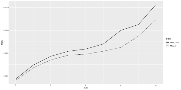
Figure 1. Models (time series (dotted line) v.s. classic (solid line)) MSEs with respect to the rank $k$.

As expected (see Figure 1), the MSE is much better with the model taking into account the time series structure. The MSE in both cases degrades when the value of the rank is increasing, the maximum being reached for $k=10$ with the value 0.0173 for the time series model compared to 0.0206 in the classic case, which still remains very low.

As we said, the estimation seems to be more precise with Gaussian errors in $\varepsilon$, and the more $\mathbf{\Theta}^{0}$ is perturbed via $\varepsilon$ or $\xi_{1},\dots,\xi_{n}$, the more the completion process is complicated and the MSE degrades. So, we now evaluate the consequence on the MSE of changing the value of $\sigma_{\varepsilon}$. For both models (with or without taking into account the time series structure), the following figure shows the evolution of the MSE with respect to $\sigma_{\varepsilon}$ when the errors in $\varepsilon$ are $\mathcal{N}(0,1/3)$ random variables and all the other parameters remain the same than previously, we are still considering 30% of observed entries.

Figure 2. Models (time series (dotted line) v.s. classic (solid line)) MSEs with respect to $\sigma_{\varepsilon}$, Gaussian errors.

Once again, as expected (see Figure 2), the MSE with time series model is smaller than the one with the classic model for each values of $\sigma_{\varepsilon}$. The fact that the MSE increases with respect to $\sigma_{\varepsilon}$ with both models illustrates that more noise always complicates the completion process. In our experiments, the values of $\sigma_{\varepsilon}$ range from 0.02 to 2. We can notice that, the more we add noise with $\sigma_{\varepsilon}$, the more significant the gap between the MSE of both models is. With $\sigma_{\varepsilon}$ equal to 2, the MSE reaches the value 0.2241 for the time series model and 0.3040 for the classic one. Our method has increasing difficulty in reconstructing the matrix when we add too much noise to the model. See also Table 4.

	Min. MSE	Max. MSE
Model w/o time series struct.	0.0023	0.3040
Model with time series struct.	0.0021	0.2241

Table 4. Min. and max. values reached by the MSE with Gaussian errors in $\varepsilon$.

Let us do the same experiment but with uniform $\mathcal{U}([-1,1])$ errors in the AR(1) processes generating the rows of $\varepsilon$.

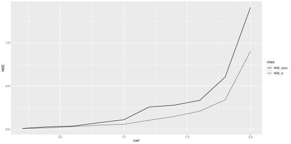
Figure 3. Models (time series (dotted line) v.s. classic (solid line)) MSEs with respect to $\sigma_{\varepsilon}$, uniform errors.

The curves shape on Figure 3 is pretty much the same as in the previous graph: the MSE for the model taking into account the time series structure is still smaller than for the classic model and this difference between the two models is even greater when we increase the value of $\sigma_{\varepsilon}$. However, this time, the MSE for both models reaches higher values, leading to a huge misestimation when $\sigma_{\varepsilon}=2$ (see Table 5).

	Min. MSE	Max. MSE
Model w/o time series struct.	0.0082	1.4088
Model with time series struct.	0.0076	0.9027

Table 5. Min. and max. values reached by the MSE with uniform errors in $\varepsilon$.

Finally, as mentioned, the previous numerical experiments were done by assuming that $k$ is known, which is mostly uncommon in practice. So, our purpose in the last part of this section is to implement the model selection method introduced at Section 4. Let us recall the criterion to minimize:

$$\left\{\begin{array}[]{rcl}\textrm{crit}(k)&=&r_{n}(\widehat{\mathbf{T}}_{k}\mathbf{\Lambda})+\textrm{pen}(k)\\ \textrm{pen}(k)&=&\mathfrak{c}_{\rm cal}k(d+\tau)\log(n)/n\end{array}\right.\textrm{$;$ }k\in\{1,\dots,20\}.$$

In the sequel, $\xi_{1},\dots,\xi_{n}\rightsquigarrow\mathcal{N}(0,0.5)$, $\varepsilon_{1,.},\dots,\varepsilon_{d,.}$ are i.i.d. AR(1) processes with $\mathcal{N}(0,1/3)$ errors, and $\sigma_{\varepsilon}=0.2$. Percentage of observed entries is still 30%. The penalty term in ${\rm crit}(.)$ depends on the constant $\mathfrak{c}_{\rm cal}>0$ which is calibrated here by using the slope heuristic presented at Section 4.
On 20 independent experiments, Table 6 gives the mean MSE obtained for the estimator computed with the true rank $k=5$ and the associated adaptative estimator computed with $\widehat{k}$ selected by minimizing the criterion studied in Section 4.

Mean MSE for $\widehat{\mathbf{T}}_{k}\mathbf{\Lambda}$	0.10712
Mean MSE for $\widehat{\mathbf{T}}_{\widehat{k}}\mathbf{\Lambda}$	0.17601

Table 6. Mean MSE over 20 simulations for $\widehat{\mathbf{T}}_{k}\mathbf{\Lambda}$ and $\widehat{\mathbf{T}}_{\widehat{k}}\mathbf{\Lambda}$.

Table 7 gives the frequence of the different values of $k$ selected. Our method select the true $k$ 8 times over 20.

k selected	4	5	6	7	8	9
Frequence	0.05	0.4	0.1	0.15	0.2	0.1

Table 7. Frequence of k-values selected

5.2. Experiments on real datas

Modern transportation data are often high-dimensional and have strong patterns including periodicity. For this reason, matrix factorization methods are very popular in this field [15, 47]. The data used in this section comes from the funFEM package (the real time data are available at https://developer.jcdecaux.com/). We used the Velib data set which contains data from the bike sharing system of Paris. These data provide the occupancy (number of available bikes/number of bike docks) of 1189 bike stations over one week. The data were collected every hour during the following period: Sunday 1st Sept. - Sunday 7th Sept., 2014. We removed the time points collected during the week-end (50 time points in total) insofar as the week-end occupancy of the bike stations differs from the week. Loading profiles of 6 different stations (week-end excluded) are represented on Figure 4.

Figure 4. Occupancy of six Velib stations over one week (week-end excluded).

We clearly notice the daily periodic behaviour of our time series. Thus, the experiments of this section are done with the real time data in the matrix $\mathbf{M}$ of dimensions $d=1189$, $\tau=25$ (which corresponds to one day) and $T=125$ (four days, from Monday to Thursday). Once again, we evaluate the MSE of the estimator with and without taking into account the time series structure, that is the periodicity in this case. Different percentages of the entries observed are tested. As for the simulated data, for the model without considering the temporal structure of our series, we apply directly our function als on the dataframe containing the observed entries with their position in the matrix, without any additional transformation on the data. The output gives directly an estimator of $\mathbf{M}$. As regards the model considering the periodic behaviour of the Velib time series in $\mathbf{M}$, the ALS optimization procedure is applied on the dataframe which has received the same transformation than the one explained at point (2) in the previous section. Once again, the output needs to be multiplied by $\mathbf{\Lambda}$ to have an estimator of $\mathbf{M}$ at the end. The MSEs obtained for both models are gathered in Table 8. We study how the MSEs vary according to the percentage of observed entries.

	15%	30%
Model w/o time series struct.	0.0609	0.0315
Model with time series struct.	0.0436	0.0381

Table 8. MSE according to the number of observed entries (%).

Of course, the real data is not exactly periodic (as can bee seen in some of the series in Figure 4. This means that the bias term of in Theorem 3.4, is larger for the method imposing periodicity than for the standard method: $\min_{{\bf T}\in\mathcal{S}_{k,\tau}}\|({\bf T}-{\bf T}^{0}){\bf\Lambda}\|_{\mathcal{F},\Pi}\geq\min_{{\bf T}\in\mathcal{S}_{k,T}}\|{\bf T}-{\bf T}^{0}\|_{\mathcal{F},\Pi}$. On the other hand, the variance term of the method using periodicity is much smaller: $k(d+\tau)/n\leq k(d+T)/n$. Thus, it is expected that when the sample size $n$ is small, using periodicity can improve on the standard method, but that this is not the case for larger values of $n$. This is perfectly illustrated by our experiments: Table 8 show that when we observe 15% of the original data, exploiting periodicity improves on the reconstruction of the data by the standard method by more than 25%. On the other hand, when we the sample size doubles, the standard method already performs slightly better.

6. Proofs

This section is organized as follows. We first state an exponential inequality that will serve as a basis for all the proofs. From this inequality, we prove Theorem 6.4, a prototype of Theorem 3.4 that holds when the set $\mathcal{S}_{k,\tau}$ is finite or infinite but compact by using $\epsilon$-nets ($\epsilon>0$). In the proof of Theorem 3.4, we provide an explicit risk-bound by using the $\epsilon$-net $\mathcal{S}_{k,\tau}^{\epsilon}$ of $\mathcal{S}_{k,\tau}$ constructed in Candès and Plan [12], Lemma 3.1.

6.1. Exponential inequality

This sections deals with the proof of the following exponential inequality, the cornerstone of the paper, which is derived from the usual Bernstein inequality and its extension to $\phi$-mixing processes due to Samson [44].

Proposition 6.1.

Let $\mathbf{T}\in S_{k,\tau}$. Under Assumptions 3.1, 3.2 and 3.3,

(6) $$\mathbb{E}\left[\exp\left(\frac{\lambda}{4}\left(\left(1+\mathfrak{c}_{\ref{preliminary_risk_bound}}\frac{\lambda}{n}\right)(R(\mathbf{T}^{0}\mathbf{\Lambda})-R(\mathbf{T}\mathbf{\Lambda}))+r_{n}(\mathbf{T}\mathbf{\Lambda})-r_{n}(\mathbf{T}^{0}\mathbf{\Lambda})\right)\right)\right]\leqslant 1$$

and

(7) $$\mathbb{E}\left[\exp\left(\frac{\lambda}{4}\left(\left(1-\mathfrak{c}_{\ref{preliminary_risk_bound}}\frac{\lambda}{n}\right)(R(\mathbf{T}\mathbf{\Lambda})-R(\mathbf{T}^{0}\mathbf{\Lambda}))+r_{n}(\mathbf{T}^{0}\mathbf{\Lambda})-r_{n}(\mathbf{T}\mathbf{\Lambda})\right)\right)\right]\leqslant 1$$

for every $\mathbf{T}\in\mathcal{S}_{k,\tau}$ and $\lambda\in(0,n\lambda^{*})$, where

$$R(\mathbf{A}):=\mathbb{E}(|Y_{1}-\langle\mathbf{X}_{1},\mathbf{A}\rangle_{\mathcal{F}}|^{2})\textrm{ $;$ }\forall\mathbf{A}\in\mathcal{M}_{d,T}(\mathbb{R}),$$

$\mathfrak{c}_{\ref{preliminary_risk_bound}}=4\max\{4\mathfrak{m}_{0}^{2},4\mathfrak{v}_{\xi},4\mathfrak{m}_{\varepsilon}^{2},2\mathfrak{m}_{\varepsilon}^{2}\Phi_{\varepsilon}^{2}\mathfrak{c}_{\Pi}\}$ and $\lambda^{*}=(16\mathfrak{m}_{0}\max\{\mathfrak{m}_{0},\mathfrak{m}_{\varepsilon},\mathfrak{c}_{\xi}\})^{-1}$.

Proof of Proposition 6.1.

The proof relies on Bernstein’s inequality as stated in [10], that we remind in the following lemma.

Lemma 6.2.

Let $T_{1},\dots,T_{n}$ be some independent and real-valued random variables. Assume that there are $v>0$ and $c>0$ such that

$$\sum_{i=1}^{n}\mathbb{E}(T_{i}^{2})\leqslant v$$

and, for any $q\geqslant 3$,

$$\sum_{i=1}^{n}\mathbb{E}(T_{i}^{q})\leqslant\frac{vc^{q-2}q!}{2}.$$

Then, for every $\lambda\in(0,1/c)$,

$$\mathbb{E}\left[\exp\left[\lambda\sum_{i=1}^{n}(T_{i}-\mathbb{E}(T_{i}))\right]\right]\leqslant\exp\left(\frac{v\lambda^{2}}{2(1-c\lambda)}\right).$$

We will also use a variant of this inequality for time series due to Samson, stated in the proof of Theorem 3 in [44].

Lemma 6.3.

Consider $m\in\mathbb{N}^{*}$, $M>0$, a stationary sequence of $\mathbb{R}^{m}$-valued random variables $Z=(Z_{t})_{t\in\mathbb{Z}}$, and

$$\Phi_{Z}:=1+\sum_{t=1}^{T}\phi_{Z}(t)^{1/2},$$

where $\phi_{Z}(t)$, $t\in\mathbb{Z}$, are the $\phi$-mixing coefficients of $Z$. For every smooth and convex function $f:[0,M]^{T}\rightarrow\mathbb{R}$ such that $\|\nabla f\|\leqslant L$ a.e, for any $\lambda>0$,

$$\mathbb{E}(\exp(\lambda(f(Z_{1},\dots,Z_{T})-\mathbb{E}[f(Z_{1},\dots,Z_{T})])))\leqslant\exp\left(\frac{\lambda^{2}L^{2}\Phi_{Z}^{2}M^{2}}{2}\right).$$

Let $\mathbf{T}\in\mathcal{S}_{k,\tau}$ be arbitrarily chosen. Consider the deterministic map $\mathbf{X}:\mathcal{E}\rightarrow\mathcal{M}_{d,T}(\mathbb{R})$ such that

$$\mathbf{X}_{i}=\mathbf{X}(\chi_{i})\textrm{ $;$ }\forall i\in\{1,\dots,n\},$$

$\Xi_{i}:=(\overline{\xi}_{i},\chi_{i})$ for any $i\in\{1,\dots,n\}$, and $h:\mathbb{R}\times\mathcal{E}\rightarrow\mathbb{R}$ the map defined by

$$h(x,y):=\frac{1}{n}(2x\langle\mathbf{X}(y),(\mathbf{T}^{0}-\mathbf{T})\mathbf{\Lambda}\rangle_{\mathcal{F}}+\langle\mathbf{X}(y),(\mathbf{T}^{0}-\mathbf{T})\mathbf{\Lambda}\rangle_{\mathcal{F}}^{2})\textrm{ $;$ }\forall(x,y)\in\mathbb{R}\times\mathcal{E}.$$

Note that

$$h(\Xi_{i}) = \frac{1}{n}(2\overline{\xi}_{i}\langle\mathbf{X}_{i},(\mathbf{T}^{0}-\mathbf{T})\mathbf{\Lambda}\rangle_{\mathcal{F}}+\langle\mathbf{X}_{i},(\mathbf{T}^{0}-\mathbf{T})\mathbf{\Lambda}\rangle_{\mathcal{F}}^{2})$$

$$= \frac{1}{n}((\overline{\xi}_{i}+\langle\mathbf{X}_{i},(\mathbf{T}^{0}-\mathbf{T})\mathbf{\Lambda}\rangle_{\mathcal{F}})^{2}-\overline{\xi}_{i}^{2})$$

$$= \frac{1}{n}((Y_{i}-\langle\mathbf{X}_{i},\mathbf{T}\mathbf{\Lambda}\rangle_{\mathcal{F}})^{2}-(Y_{i}-\langle\mathbf{X}_{i},\mathbf{T}^{0}\mathbf{\Lambda}\rangle_{\mathcal{F}})^{2})$$

and

$$\sum_{i=1}^{n}(h(\Xi_{i})-\mathbb{E}(h(\Xi_{i})))=r_{n}(\mathbf{T}\mathbf{\Lambda})-r_{n}(\mathbf{T}^{0}\mathbf{\Lambda})+R(\mathbf{T}^{0}\mathbf{\Lambda})-R(\mathbf{T}\mathbf{\Lambda}).$$

Now, replacing $\overline{\xi}_{i}$ by its expression in terms of $\mathbf{X}_{i}$, $\xi_{i}$ and $\varepsilon$,

$$\sum_{i=1}^{n}(h(\Xi_{i})-\mathbb{E}(h(\Xi_{i}))) = \sum_{i=1}^{n}\left(\frac{2}{n}\xi_{i}\langle\mathbf{X}_{i},(\mathbf{T}^{0}-\mathbf{T})\mathbf{\Lambda}\rangle_{\mathcal{F}}\right)$$

$$+\sum_{i=1}^{n}\left(\frac{2}{n}\langle\mathbf{X}_{i},\varepsilon\rangle_{\mathcal{F}}\langle\mathbf{X}_{i},(\mathbf{T}^{0}-\mathbf{T})\mathbf{\Lambda}\rangle_{\mathcal{F}}\right)$$

$$+\sum_{i=1}^{n}\left(\frac{1}{n}\langle\mathbf{X}_{i},(\mathbf{T}^{0}-\mathbf{T})\mathbf{\Lambda}\rangle_{\mathcal{F}}^{2}-\mathbb{E}(h(\Xi_{i}))\right)$$

$$=: \sum_{i=1}^{n}A_{i}+\sum_{i=1}^{n}B_{i}+\sum_{i=1}^{n}(C_{i}-\mathbb{E}(h(\Xi_{i}))).$$

In order to conclude, by using Lemmas 6.2 and 6.3, let us provide suitable bounds for the exponentiel moments of each terms of the previous decomposition:

• Bounds for the $A_{i}$’s and the $C_{i}$’s. First, note that since $\mathbf{X}_{1}$, $\xi_{1}$ and $\varepsilon$ are independent,

  (8) $$R(\mathbf{T}\mathbf{\Lambda})-R(\mathbf{T}^{0}\mathbf{\Lambda}) = \mathbb{E}((Y_{1}-\langle\mathbf{X}_{1},\mathbf{T}\mathbf{\Lambda}\rangle_{\mathcal{F}})^{2}-(Y_{1}-\langle\mathbf{X}_{1},\mathbf{T}^{0}\mathbf{\Lambda}\rangle_{\mathcal{F}})^{2})$$

  $$= 2\mathbb{E}(\overline{\xi}_{1}\langle\mathbf{X}_{1},(\mathbf{T}^{0}-\mathbf{T})\mathbf{\Lambda}\rangle_{\mathcal{F}})+\mathbb{E}(\langle\mathbf{X}_{1},(\mathbf{T}^{0}-\mathbf{T})\mathbf{\Lambda}\rangle_{\mathcal{F}}^{2})$$

  $$= 2\langle\mathbb{E}(\langle\mathbf{X}_{1},(\mathbf{T}^{0}-\mathbf{T})\mathbf{\Lambda}\rangle_{\mathcal{F}}\mathbf{X}_{1}),\mathbb{E}(\varepsilon)\rangle_{\mathcal{F}}$$

  $$+2\mathbb{E}(\xi_{1})\mathbb{E}(\langle\mathbf{X}_{1},(\mathbf{T}^{0}-\mathbf{T})\mathbf{\Lambda}\rangle_{\mathcal{F}})+\|(\mathbf{T}^{0}-\mathbf{T})\mathbf{\Lambda}\|_{\mathcal{F},\Pi}^{2}$$

  $$= \|(\mathbf{T}^{0}-\mathbf{T})\mathbf{\Lambda}\|_{\mathcal{F},\Pi}^{2}.$$

  On the one hand,

  $$\mathbb{E}(A_{i}^{2})\leqslant\frac{4}{n^{2}}\mathbb{E}(\xi_{i}^{2})\mathbb{E}(\langle\mathbf{X}_{i},(\mathbf{T}^{0}-\mathbf{T})\mathbf{\Lambda}\rangle_{\mathcal{F}}^{2})\leqslant\frac{4}{n^{2}}\mathfrak{v}_{\xi}(R(\mathbf{T}^{0}\mathbf{\Lambda})-R(\mathbf{T}\mathbf{\Lambda}))$$

  thanks to Equality (8). Moreover,

  $$\mathbb{E}(|A_{i}|^{q}) \leqslant \frac{2^{q}}{n^{q}}\mathbb{E}(|\xi_{i}|^{q})\mathbb{E}(\langle\mathbf{X}_{i},(\mathbf{T}^{0}-\mathbf{T})\mathbf{\Lambda}\rangle_{\mathcal{F}}^{q})$$

  $$\leqslant \left(\frac{4\mathfrak{c}_{\xi}\mathfrak{m}_{0}}{n}\right)^{q-2}\frac{q!}{2}\cdot\frac{4\mathfrak{v}_{\xi}}{n^{2}}(R(\mathbf{T}^{0}\mathbf{\Lambda})-R(\mathbf{T}\mathbf{\Lambda})).$$

  So, we can use Lemma 6.2 with

  $$v=\frac{4}{n}\mathfrak{v}_{\xi}(R(\mathbf{T}^{0}\mathbf{\Lambda})-R(\mathbf{T}\mathbf{\Lambda}))\textrm{ and }c=\frac{4\mathfrak{c}_{\xi}\mathfrak{m}_{0}}{n}$$

  to obtain:

  $$\mathbb{E}\left[\exp\left(\lambda\sum_{i=1}^{n}A_{i}\right)\right]\leqslant\exp\left[\frac{2\mathfrak{v}_{\xi}(R(\mathbf{T}^{0}\mathbf{\Lambda})-R(\mathbf{T}\mathbf{\Lambda}))\lambda^{2}}{n-4\mathfrak{c}_{\xi}\mathfrak{m}_{0}\lambda}\right]$$

  for any $\lambda\in(0,n/(4\mathfrak{c}_{\xi}\mathfrak{m}_{0}))$. On the other hand, $|C_{i}|\leqslant 4\mathfrak{m}_{0}^{2}/n$ and

  $$\mathbb{E}(C_{i}^{2})=\frac{1}{n^{2}}\mathbb{E}(\langle\mathbf{X}_{i},(\mathbf{T}^{0}-\mathbf{T})\mathbf{\Lambda}\rangle_{\mathcal{F}}^{4})\leqslant\frac{4\mathfrak{m}_{0}^{2}}{n^{2}}\|(\mathbf{T}^{0}-\mathbf{T})\mathbf{\Lambda}\|_{\mathcal{F},\Pi}^{2}=\frac{4}{n^{2}}\mathfrak{m}_{0}^{2}(R(\mathbf{T}^{0}\mathbf{\Lambda})-R(\mathbf{T}\mathbf{\Lambda}))$$

  thanks to Equality (8). So, we can use Lemma 6.2 with

  $$v=\frac{4}{n}\mathfrak{m}_{0}^{2}(R(\mathbf{T}^{0}\mathbf{\Lambda})-R(\mathbf{T}\mathbf{\Lambda}))\textrm{ and }c=\frac{4\mathfrak{m}_{0}^{2}}{n}$$

  to obtain:

  $$\mathbb{E}\left[\exp\left(\lambda\sum_{i=1}^{n}(C_{i}-\mathbb{E}(h(\Xi_{i})))\right)\right]\leqslant\exp\left[\frac{2\mathfrak{m}_{0}^{2}(R(\mathbf{T}^{0}\mathbf{\Lambda})-R(\mathbf{T}\mathbf{\Lambda}))\lambda^{2}}{n-4\mathfrak{m}_{0}^{2}\lambda}\right]$$

  for any $\lambda\in(0,n/(4\mathfrak{m}_{0}^{2}))$.

• Bounds for the $B_{i}$’s. First, write

  $$\sum_{i=1}^{n}B_{i}=\sum_{i=1}^{n}(B_{i}-\mathbb{E}(B_{i}|\varepsilon))+\sum_{i=1}^{n}\mathbb{E}(B_{i}|\varepsilon)=:\sum_{i=1}^{n}D_{i}+\sum_{i=1}^{n}E_{i},$$

  and note that

  $$\mathbb{E}(B_{i}|\varepsilon) = \frac{2}{n}\mathbb{E}(\langle\mathbf{X}_{i},\varepsilon\rangle_{\mathcal{F}}\langle\mathbf{X}_{i},(\mathbf{T}^{0}-\mathbf{T})\mathbf{\Lambda}\rangle_{\mathcal{F}}|\varepsilon)$$

  $$= \frac{2}{n}\sum_{j,t}\mathbb{E}(\mathbf{1}_{\chi_{i}=(j,t)}[(\mathbf{T}^{0}-\mathbf{T})\mathbf{\Lambda}]_{\chi_{i}})\varepsilon_{j,t}=\frac{2}{n}\sum_{j,t}p_{j,t}[(\mathbf{T}^{0}-\mathbf{T})\mathbf{\Lambda}]_{j,t}\varepsilon_{j,t}$$

  and

  (10) $$\|(\mathbf{T}^{0}-\mathbf{T})\mathbf{\Lambda}\|_{\mathcal{F},\Pi}^{2}=\mathbb{E}(\langle\mathbf{X}_{i},(\mathbf{T}^{0}-\mathbf{T})\mathbf{\Lambda}\rangle_{\mathcal{F}}^{2})=\mathbb{E}([(\mathbf{T}^{0}-\mathbf{T})\mathbf{\Lambda}]_{\chi_{i}}^{2})=\sum_{j,t}p_{j,t}[(\mathbf{T}^{0}-\mathbf{T})\mathbf{\Lambda}]_{j,t}^{2},$$

  where

  $$p_{j,t}:=\mathbb{P}(\chi_{1}=(j,t))=\Pi(\{e_{\mathbb{R}^{d}}(j)e_{\mathbb{R}^{T}}(t)^{*}\})$$

  for every $(j,t)\in\mathcal{E}$. On the one hand, given $\varepsilon$, the $D_{i}$’s are i.i.d, $|D_{i}|\leqslant 8\mathfrak{m}_{\varepsilon}\mathfrak{m}_{0}/n$ and

  $$\mathbb{E}(B_{i}^{2}|\varepsilon) =\frac{4}{n^{2}}\mathbb{E}(\langle\mathbf{X}_{i},\varepsilon\rangle_{\mathcal{F}}^{2}\langle\mathbf{X}_{i},(\mathbf{T}^{0}-\mathbf{T})\mathbf{\Lambda}\rangle_{\mathcal{F}}^{2}|\varepsilon)$$

  $$\leqslant\frac{4}{n^{2}}\mathfrak{m}_{\varepsilon}^{2}\mathbb{E}(\langle\mathbf{X}_{i},(\mathbf{T}^{0}-\mathbf{T})\mathbf{\Lambda}\rangle_{\mathcal{F}}^{2}|\varepsilon)=\frac{4}{n^{2}}\mathfrak{m}_{\varepsilon}^{2}\mathbb{E}(\langle\mathbf{X}_{i},(\mathbf{T}^{0}-\mathbf{T})\mathbf{\Lambda}\rangle_{\mathcal{F}}^{2})=\frac{4}{n^{2}}\mathfrak{m}_{\varepsilon}^{2}(R(\mathbf{T}^{0}\mathbf{\Lambda})-R(\mathbf{T}\mathbf{\Lambda}))$$

  thanks to Equality (8). So, conditionnally on $\varepsilon$, we can apply Lemma 6.2 with

  $$v=\frac{4}{n}\mathfrak{m}_{\varepsilon}^{2}(R(\mathbf{T}^{0}\mathbf{\Lambda})-R(\mathbf{T}\mathbf{\Lambda}))\textrm{ and }c=\frac{8\mathfrak{m}_{\varepsilon}\mathfrak{m}_{0}}{n}$$

  to obtain:

  $$\mathbb{E}\left[\left.\exp\left(\lambda\sum_{i=1}^{n}D_{i}\right)\right|\varepsilon\right]\leqslant\exp\left[\frac{2\mathfrak{m}_{\varepsilon}^{2}(R(\mathbf{T}^{0}\mathbf{\Lambda})-R(\mathbf{T}\mathbf{\Lambda}))\lambda^{2}}{n-8\mathfrak{m}_{\varepsilon}\mathfrak{m}_{0}\lambda}\right]$$

  for any $\lambda\in(0,n/(8\mathfrak{m}_{\varepsilon}\mathfrak{m}_{0}))$. Taking the expectation of both sides gives:

  $$\mathbb{E}\left[\exp\left(\lambda\sum_{i=1}^{n}D_{i}\right)\right]\leqslant\exp\left[\frac{2\mathfrak{m}_{\varepsilon}^{2}(R(\mathbf{T}^{0}\mathbf{\Lambda})-R(\mathbf{T}\mathbf{\Lambda}))\lambda^{2}}{n-8\mathfrak{m}_{\varepsilon}\mathfrak{m}_{0}\lambda}\right].$$

  On the other hand, let us focus on the $E_{i}$’s. Thanks to Equality (• ‣ 6.1) and since the rows of $\varepsilon$ are independent,

  $$\mathbb{E}\left[\exp\left(\lambda\sum_{i=1}^{n}E_{i}\right)\right] = \mathbb{E}\left[\exp\left[2\lambda\sum_{j,t}p_{j,t}[(\mathbf{T}^{0}-\mathbf{T})\mathbf{\Lambda}]_{j,t}\varepsilon_{j,t}\right]\right]$$

  $$= \prod_{j=1}^{d}\mathbb{E}\left[\exp\left(2\lambda\sum_{t=1}^{T}p_{j,t}[(\mathbf{T}^{0}-\mathbf{T})\mathbf{\Lambda}]_{j,t}\varepsilon_{j,t}\right)\right].$$

  Now, for any $j\in\{1,\dots,d\}$, let us apply Lemma 6.3 to $(\varepsilon_{j,1},\dots,\varepsilon_{j,T})$, which is a sample of a $\phi$-mixing sequence, and to the function $f_{j}:[0,\mathfrak{m}_{\varepsilon}]^{T}\rightarrow\mathbb{R}$ defined by

  $$f_{j}(u_{1},\dots,u_{T}):=2\sum_{t=1}^{T}p_{j,t}[(\mathbf{T}^{0}-\mathbf{T})\mathbf{\Lambda}]_{j,t}u_{t}\textrm{ $;$ }\forall u\in[0,\mathfrak{m}_{\varepsilon}]^{T}.$$

  Since

  $$\|\nabla f_{j}(u_{1},\dots,u_{T})\|^{2}=4\sum_{t=1}^{T}p_{j,t}^{2}[(\mathbf{T}^{0}-\mathbf{T})\mathbf{\Lambda}]_{j,t}^{2}\textrm{ $;$ }\forall u\in[0,\mathfrak{m}_{\varepsilon}]^{T},$$

  by Lemma 6.3:

  $$\mathbb{E}\left[\exp\left(2\lambda\sum_{t=1}^{T}p_{j,t}[(\mathbf{T}^{0}-\mathbf{T})\mathbf{\Lambda}]_{j,t}\varepsilon_{j,t}\right)\right] = \mathbb{E}(\exp(\lambda(f_{j}(\varepsilon_{j,1},\dots,\varepsilon_{j,T})-\mathbb{E}[f_{j}(\varepsilon_{j,1},\dots,\varepsilon_{j,T})])))$$

  $$\leqslant \exp\left(2\mathfrak{m}_{\varepsilon}^{2}\lambda^{2}\Phi_{\varepsilon}^{2}\sum_{t=1}^{T}p_{j,t}^{2}[(\mathbf{T}^{0}-\mathbf{T})\mathbf{\Lambda}]_{j,t}^{2}\right).$$

  Thus, for any $\lambda>0$, by Equalities (8) and (10) together with $n\leqslant dT$,

  $$\mathbb{E}\left[\exp\left(\lambda\sum_{i=1}^{n}E_{i}\right)\right] =\prod_{j=1}^{d}\mathbb{E}\left[\exp\left(2\lambda\sum_{t=1}^{T}p_{j,t}[(\mathbf{T}^{0}-\mathbf{T})\mathbf{\Lambda}]_{j,t}\varepsilon_{j,t}\right)\right]$$

  $$\leqslant\prod_{j=1}^{d}\exp\left(2\mathfrak{m}_{\varepsilon}^{2}\lambda^{2}\Phi_{\varepsilon}^{2}\sum_{t=1}^{T}p_{j,t}^{2}[(\mathbf{T}^{0}-\mathbf{T})\mathbf{\Lambda}]_{j,t}^{2}\right)$$

  $$\leqslant\exp\left[\frac{2\mathfrak{m}_{\varepsilon}^{2}\lambda^{2}\Phi_{\varepsilon}^{2}\mathfrak{c}_{\Pi}}{dT}\sum_{j,t}p_{j,t}[(\mathbf{T}^{0}-\mathbf{T})\mathbf{\Lambda}]_{j,t}^{2}\right]\leqslant\exp\left[\frac{2\mathfrak{m}_{\varepsilon}^{2}\lambda^{2}\Phi_{\varepsilon}^{2}\mathfrak{c}_{\Pi}}{n}(R(\mathbf{T}^{0}\mathbf{\Lambda})-R(\mathbf{T}\mathbf{\Lambda}))\right].$$

Therefore, these bounds together with Jensen’s inequality give:

$$\mathbb{E}\exp \left(\frac{\lambda}{4}[r_{n}(\mathbf{T}\mathbf{\Lambda})-r_{n}(\mathbf{T}^{0}\mathbf{\Lambda})+R(\mathbf{T}^{0}\mathbf{\Lambda})-R(\mathbf{T}\mathbf{\Lambda})]\right)$$

$$=\mathbb{E}\left[\exp\left(\frac{\lambda}{4}\sum_{i=1}^{n}(h(\Xi_{i})-\mathbb{E}(h(\Xi_{i})))\right)\right]$$

$$=\mathbb{E}\left[\exp\left(\frac{\lambda}{4}\sum_{i=1}^{n}A_{i}+\frac{\lambda}{4}\sum_{i=1}^{n}(C_{i}-\mathbb{E}(h(\Xi_{i})))+\frac{\lambda}{4}\sum_{i=1}^{n}D_{i}+\frac{\lambda}{4}\sum_{i=1}^{n}E_{i}\right)\right]$$

$$\leqslant\frac{1}{4}\left[\mathbb{E}\left[\exp\left(\lambda\sum_{i=1}^{n}A_{i}\right)\right]+\mathbb{E}\left[\exp\left(\lambda\sum_{i=1}^{n}(C_{i}-\mathbb{E}(h(\Xi_{i})))\right)\right]\right.$$

$$\quad+\left.\mathbb{E}\left[\exp\left(\lambda\sum_{i=1}^{n}D_{i}\right)\right]+\mathbb{E}\left[\exp\left(\lambda\sum_{i=1}^{n}E_{i}\right)\right]\right]$$

$$\leqslant\exp\left[\frac{2\mathfrak{v}_{\xi}}{1-4\mathfrak{c}_{\xi}\mathfrak{m}_{0}\lambda/n}\cdot\frac{\lambda^{2}}{n}(R(\mathbf{T}^{0}\mathbf{\Lambda})-R(\mathbf{T}\mathbf{\Lambda}))\right]+\exp\left[\frac{2\mathfrak{m}_{0}^{2}}{1-4\mathfrak{m}_{0}^{2}\lambda/n}\cdot\frac{\lambda^{2}}{n}(R(\mathbf{T}^{0}\mathbf{\Lambda})-R(\mathbf{T}\mathbf{\Lambda}))\right]$$

$$\quad+\exp\left[\frac{2\mathfrak{m}_{\varepsilon}^{2}}{1-8\mathfrak{m}_{\varepsilon}\mathfrak{m}_{0}\lambda/n}\cdot\frac{\lambda^{2}}{n}(R(\mathbf{T}^{0}\mathbf{\Lambda})-R(\mathbf{T}\mathbf{\Lambda}))\right]+\exp\left[2\mathfrak{m}_{\varepsilon}^{2}\Phi_{\varepsilon}^{2}\mathfrak{c}_{\Pi}\frac{\lambda^{2}}{n}(R(\mathbf{T}^{0}\mathbf{\Lambda})-R(\mathbf{T}\mathbf{\Lambda}))\right]$$

$$\leqslant\exp\left[\mathfrak{c}_{\lambda}\frac{\lambda^{2}}{n}(R(\mathbf{T}^{0}\mathbf{\Lambda})-R(\mathbf{T}\mathbf{\Lambda}))\right]$$

with

$$\mathfrak{c}_{\lambda}=\max\left\{\frac{2\mathfrak{v}_{\xi}}{1-4\mathfrak{c}_{\xi}\mathfrak{m}_{0}\lambda/n},\frac{2\mathfrak{m}_{0}^{2}}{1-4\mathfrak{m}_{0}^{2}\lambda/n},\frac{2\mathfrak{m}_{\varepsilon}^{2}}{1-8\mathfrak{m}_{\varepsilon}\mathfrak{m}_{0}\lambda/n},2\mathfrak{m}_{\varepsilon}^{2}\Phi_{\varepsilon}^{2}\mathfrak{c}_{\Pi}\right\}$$

and

$$0<\lambda<n\min\left\{\frac{1}{4\mathfrak{c}_{\xi}\mathfrak{m}_{0}},\frac{1}{4\mathfrak{m}_{0}^{2}},\frac{1}{8\mathfrak{m}_{\varepsilon}\mathfrak{m}_{0}}\right\}.$$

In particular, for

$$\lambda<\frac{n}{16\mathfrak{m}_{0}\max\{\mathfrak{m}_{0},\mathfrak{m}_{\varepsilon},\mathfrak{c}_{\xi}\}},$$

we have

$$\mathfrak{c}_{\lambda}\leqslant\max\{4\mathfrak{m}_{0}^{2},4\mathfrak{v}_{\xi},4\mathfrak{m}_{\varepsilon}^{2},2\mathfrak{m}_{\varepsilon}^{2}\Phi_{\varepsilon}^{2}\mathfrak{c}_{\Pi}\}.$$

This ends the proof of the first inequality. ∎

6.2. A preliminary non-explicit risk bound

We now provide a simpler version of Theorem 3.4, that holds in the case where $\mathcal{S}_{k,\tau}$ is finite: (1) in the following theorem. When this is not the case, we provide a similar bound using a general $\epsilon$-net, that is (2) in the theorem.

Theorem 6.4.

Consider $\alpha\in]0,1[$.

1. Under Assumptions 3.1, 3.2 and 3.3, if $|\mathcal{S}_{k,\tau}|<\infty$, then

   $$\|\widehat{\mathbf{\Theta}}_{k,\tau}-\mathbf{\Theta}^{0}\|_{\mathcal{F},\Pi}^{2}\leqslant 3\min_{\mathbf{T}\in\mathcal{S}_{k,\tau}}\|(\mathbf{T}-\mathbf{T}^{0})\mathbf{\Lambda}\|_{\mathcal{F},\Pi}^{2}+\frac{\mathfrak{c}_{\ref{risk_bound},1}}{n}\log\left(\frac{2}{\alpha}|\mathcal{S}_{k,\tau}|\right)$$

   with probability larger than $1-\alpha$, where $\mathfrak{c}_{\ref{risk_bound},1}=32(\mathfrak{c}_{\ref{preliminary_risk_bound}}^{-1}\wedge\lambda^{*})^{-1}$.

2. Under Assumptions 3.1, 3.2 and 3.3, for every $\epsilon>0$, there exists a finite subset $\mathcal{S}_{k,\tau}^{\epsilon}$ of $\mathcal{S}_{k,\tau}$ such that

   $$\|\widehat{\mathbf{\Theta}}_{k,\tau}-\mathbf{\Theta}^{0}\|_{\mathcal{F},\Pi}^{2}\leqslant 3\min_{\mathbf{T}\in\mathcal{S}_{k,\tau}}\|(\mathbf{T}-\mathbf{T}^{0})\mathbf{\Lambda}\|_{\mathcal{F},\Pi}^{2}+\frac{\mathfrak{c}_{\ref{risk_bound},1}}{n}\log\left(\frac{2}{\alpha}|\mathcal{S}_{k,\tau}^{\epsilon}|\right)+\left[\mathfrak{c}_{\ref{risk_bound},2}+8\mathfrak{m}_{\mathbf{\Lambda}}\mathfrak{c}_{\xi}\log\left(\frac{1}{\alpha}\right)\right]\epsilon$$

   with probability larger than $1-\alpha$, where $\mathfrak{c}_{\ref{risk_bound},2}=4\mathfrak{m}_{\mathbf{\Lambda}}(\mathfrak{v}_{\xi}^{1/2}+\mathfrak{v}_{\xi}/(2\mathfrak{c}_{\xi})+\mathfrak{m}_{\varepsilon}+3\mathfrak{m}_{0})$.

Proof of Theorem 6.4.

1. Assume that $|\mathcal{S}_{k,\tau}|<\infty$. For any $x>0$, $\lambda\in(0,n\lambda^{*})$ and $\mathcal{S}\subset\mathcal{M}_{d,\tau}(\mathbb{R})$, consider the events

   $$\Omega_{x,\lambda,\mathcal{S}}^{-}(\mathbf{T}):=\left\{\left(1-\mathfrak{c}_{\ref{preliminary_risk_bound}}\frac{\lambda}{n}\right)\|(\mathbf{T}-\mathbf{T}^{0})\mathbf{\Lambda}\|_{\mathcal{F},\Pi}^{2}-(r_{n}(\mathbf{T}\mathbf{\Lambda})-r_{n}(\mathbf{T}^{0}\mathbf{\Lambda}))>4x\right\}\textrm{, }\mathbf{T}\in\mathcal{S}$$

   and

   $$\Omega_{x,\lambda,\mathcal{S}}^{-}:=\bigcup_{\mathbf{T}\in\mathcal{S}}\Omega_{x,\lambda,\mathcal{S}}^{-}(\mathbf{T}).$$

   By Markov’s inequality together with Proposition 6.1, Inequality (7),

   $$\mathbb{P}(\Omega_{x,\lambda,\mathcal{S}_{k,\tau}}^{-}) \leqslant \sum_{\mathbf{T}\in\mathcal{S}_{k,\tau}}\mathbb{P}\left(\exp\left(\frac{\lambda}{4}\left(\left(1-\mathfrak{c}_{\ref{preliminary_risk_bound}}\frac{\lambda}{n}\right)(R(\mathbf{T}\mathbf{\Lambda})-R(\mathbf{T}^{0}\mathbf{\Lambda}))-(r_{n}(\mathbf{T}\mathbf{\Lambda})-r_{n}(\mathbf{T}^{0}\mathbf{\Lambda}))\right)\right)>e^{\lambda x}\right)$$

   $$\leqslant |\mathcal{S}_{k,\tau}|e^{-\lambda x}.$$

   In the same way, with

   $$\Omega_{x,\lambda,\mathcal{S}}^{+}(\mathbf{T}):=\left\{-\left(1+\mathfrak{c}_{\ref{preliminary_risk_bound}}\frac{\lambda}{n}\right)\|(\mathbf{T}-\mathbf{T}^{0})\mathbf{\Lambda}\|_{\mathcal{F},\Pi}^{2}+r_{n}(\mathbf{T}\mathbf{\Lambda})-r_{n}(\mathbf{T}^{0}\mathbf{\Lambda})>4x\right\}\textrm{, }\mathbf{T}\in\mathcal{S}$$

   and

   $$\Omega_{x,\lambda,\mathcal{S}}^{+}:=\bigcup_{\mathbf{T}\in\mathcal{S}}\Omega_{x,\lambda,\mathcal{S}}^{+}(\mathbf{T}),$$

   by Markov’s inequality together with Proposition 6.1, Inequality (6), $\mathbb{P}(\Omega_{x,\lambda,\mathcal{S}_{k,\tau}}^{+})\leqslant|\mathcal{S}_{k,\tau}|e^{-\lambda x}$. Then,

   $$\mathbb{P}(\Omega_{x,\lambda,\mathcal{S}_{k,\tau}})\geqslant 1-2|\mathcal{S}_{k,\tau}|e^{-\lambda x}$$

   with

   $$\Omega_{x,\lambda,\mathcal{S}}:=(\Omega_{x,\lambda,\mathcal{S}}^{-})^{c}\cap(\Omega_{x,\lambda,\mathcal{S}}^{+})^{c}\subset\Omega_{x,\lambda,\mathcal{S}}^{-}(\widehat{\mathbf{T}}_{k,\tau})^{c}\cap\Omega_{x,\lambda,\mathcal{S}}^{+}(\widehat{\mathbf{T}}_{k,\tau})^{c}=:\Omega_{x,\lambda,\mathcal{S}_{k,\tau}}(\widehat{\mathbf{T}}_{k,\tau}).$$

   Moreover, on the event $\Omega_{x,\lambda,\mathcal{S}_{k,\tau}}$, by the definition of $\widehat{\mathbf{T}}_{k,\tau}$,

   $$\|\widehat{\mathbf{\Theta}}_{k,\tau}-\mathbf{\Theta}^{0}\|_{\mathcal{F},\Pi}^{2} \leqslant \left(1-\mathfrak{c}_{\ref{preliminary_risk_bound}}\frac{\lambda}{n}\right)^{-1}(r_{n}(\widehat{\mathbf{T}}_{k,\tau}\mathbf{\Lambda})-r_{n}(\mathbf{T}^{0}\mathbf{\Lambda})+4x)$$

   $$= \left(1-\mathfrak{c}_{\ref{preliminary_risk_bound}}\frac{\lambda}{n}\right)^{-1}\left(\min_{\mathbf{T}\in\mathcal{S}_{k,\tau}}\{r_{n}(\mathbf{T}\mathbf{\Lambda})-r_{n}(\mathbf{T}^{0}\mathbf{\Lambda})\}+4x\right)$$

   $$\leqslant \frac{1+\mathfrak{c}_{\ref{preliminary_risk_bound}}\lambda n^{-1}}{1-\mathfrak{c}_{\ref{preliminary_risk_bound}}\lambda n^{-1}}\min_{\mathbf{T}\in\mathcal{S}_{k,\tau}}\|(\mathbf{T}-\mathbf{T}^{0})\mathbf{\Lambda}\|_{\mathcal{F},\Pi}^{2}+\frac{8x}{1-\mathfrak{c}_{\ref{preliminary_risk_bound}}\lambda n^{-1}}.$$

   So, for any $\alpha\in]0,1[$, with probability larger than $1-\alpha$,

   $$\|\widehat{\mathbf{\Theta}}_{k,\tau}-\mathbf{\Theta}^{0}\|_{\mathcal{F},\Pi}^{2}\leqslant\frac{1+\mathfrak{c}_{\ref{preliminary_risk_bound}}\lambda n^{-1}}{1-\mathfrak{c}_{\ref{preliminary_risk_bound}}\lambda n^{-1}}\min_{\mathbf{T}\in\mathcal{S}_{k,\tau}}\|(\mathbf{T}-\mathbf{T}^{0})\mathbf{\Lambda}\|_{\mathcal{F},\Pi}^{2}+\frac{8\lambda^{-1}\log(2\alpha^{-1}|\mathcal{S}_{k,\tau}|)}{1-\mathfrak{c}_{\ref{preliminary_risk_bound}}\lambda n^{-1}}.$$

   Now, let us take

   $$\lambda=\frac{n}{2}\left(\frac{1}{\mathfrak{c}_{\ref{preliminary_risk_bound}}}\wedge\lambda^{*}\right)\in(0,n\lambda^{*})\textrm{ and }x=\frac{1}{\lambda}\log\left(\frac{2}{\alpha}|\mathcal{S}_{k,\tau}|\right).$$

   In particular, $\mathfrak{c}_{\ref{preliminary_risk_bound}}\lambda n^{-1}\leqslant 1/2$, and then

   $$\frac{1+\mathfrak{c}_{\ref{preliminary_risk_bound}}\lambda n^{-1}}{1-\mathfrak{c}_{\ref{preliminary_risk_bound}}\lambda n^{-1}}\leqslant 3\textrm{ and }\frac{8\lambda^{-1}}{1-\mathfrak{c}_{\ref{preliminary_risk_bound}}\lambda n^{-1}}\leqslant 32\left(\frac{1}{\mathfrak{c}_{\ref{preliminary_risk_bound}}}\wedge\lambda^{*}\right)^{-1}\frac{1}{n}.$$

   Therefore, with probability larger than $1-\alpha$,

   $$\|\widehat{\mathbf{\Theta}}_{k,\tau}-\mathbf{\Theta}^{0}\|_{\mathcal{F},\Pi}^{2}\leqslant 3\min_{\mathbf{T}\in\mathcal{S}_{k,\tau}}\|(\mathbf{T}-\mathbf{T}^{0})\mathbf{\Lambda}\|_{\mathcal{F},\Pi}^{2}+32\left(\frac{1}{\mathfrak{c}_{\ref{preliminary_risk_bound}}}\wedge\lambda^{*}\right)^{-1}\frac{1}{n}\log\left(\frac{2}{\alpha}|\mathcal{S}_{k,\tau}|\right).$$

2. Now, assume that $|\mathcal{S}_{k,\tau}|=\infty$. Since $\textrm{dim}(\mathcal{M}_{d,\tau}(\mathbb{R}))<\infty$ and $\mathcal{S}_{k,\tau}$ is a bounded subset of $\mathcal{M}_{d,\tau}(\mathbb{R})$ (equipped with $\mathbf{T}\mapsto\sup_{j,t}|\mathbf{T}_{j,t}|$), $\mathcal{S}_{k,\tau}$ is compact in $(\mathcal{M}_{d,\tau}(\mathbb{R}),\|.\|_{\mathcal{F}})$. Then, for any $\epsilon>0$, there exists a finite subset $\mathcal{S}_{k,\tau}^{\epsilon}$ of $\mathcal{S}_{k,\tau}$ such that

   (11) $$\forall\mathbf{T}\in\mathcal{S}_{k,\tau},\exists\mathbf{T}^{\epsilon}\in\mathcal{S}_{k,\tau}^{\epsilon}:\|\mathbf{T}-\mathbf{T}^{\epsilon}\|_{\mathcal{F}}\leqslant\epsilon.$$

   On the one hand, for any $\mathbf{T}\in\mathcal{S}_{k,\tau}$ and $\mathbf{T}^{\epsilon}\in\mathcal{S}_{k,\tau}^{\epsilon}$ satisfying (11), since $\langle\mathbf{X}_{i},(\mathbf{T}-\mathbf{T}^{\epsilon})\mathbf{\Lambda}\rangle_{\mathcal{F}}=\langle\mathbf{X}_{i}\mathbf{\Lambda}^{*},\mathbf{T}-\mathbf{T}^{\epsilon}\rangle_{\mathcal{F}}$ for every $i\in\{1,\dots,n\}$,

   (12) $$|r_{n}(\mathbf{T}\mathbf{\Lambda})-r_{n}(\mathbf{T}^{\epsilon}\mathbf{\Lambda})| \leqslant \frac{1}{n}\sum_{i=1}^{n}|\langle\mathbf{X}_{i},(\mathbf{T}-\mathbf{T}^{\epsilon})\mathbf{\Lambda}\rangle_{\mathcal{F}}(2Y_{i}-\langle\mathbf{X}_{i},(\mathbf{T}+\mathbf{T}^{\epsilon})\mathbf{\Lambda}\rangle_{\mathcal{F}})|$$

   $$\leqslant \frac{\epsilon}{n}\sum_{i=1}^{n}\|\mathbf{X}_{i}\mathbf{\Lambda}^{*}\|_{\mathcal{F}}\left(2|Y_{i}|+\sup_{j,t}\left|\sum_{\ell=1}^{\tau}(\mathbf{T}+\mathbf{T}^{\epsilon})_{j,\ell}\mathbf{\Lambda}_{\ell,t}\right|\right)$$

   $$\leqslant \epsilon\mathfrak{m}_{\mathbf{\Lambda}}\left(\frac{2}{n}\sum_{i=1}^{n}|Y_{i}|+2\mathfrak{m}_{0}\right)\leqslant\mathfrak{c}_{1}(\xi_{1},\dots,\xi_{n})\epsilon$$

   with

   $$\mathfrak{c}_{1}(\xi_{1},\dots,\xi_{n}):=2\mathfrak{m}_{\mathbf{\Lambda}}\left(\frac{1}{n}\sum_{i=1}^{n}|\xi_{i}|+\mathfrak{m}_{\varepsilon}+2\mathfrak{m}_{0}\right),$$

   and thanks to Equality (8),

   (13) $$|R(\mathbf{T}\mathbf{\Lambda})-R(\mathbf{T}^{\epsilon}\mathbf{\Lambda})| = |R(\mathbf{T}\mathbf{\Lambda})-R(\mathbf{T}^{0}\mathbf{\Lambda})-(R(\mathbf{T}^{\epsilon}\mathbf{\Lambda})-R(\mathbf{T}^{0}\mathbf{\Lambda}))|$$

   $$= |\|(\mathbf{T}-\mathbf{T}^{0})\mathbf{\Lambda}\|_{\mathcal{F},\Pi}^{2}-\|(\mathbf{T}^{\epsilon}-\mathbf{T}^{0})\mathbf{\Lambda}\|_{\mathcal{F},\Pi}^{2}|$$

   $$\leqslant \mathbb{E}(|\langle\mathbf{X}_{i},(\mathbf{T}-\mathbf{T}^{\epsilon})\mathbf{\Lambda}\rangle_{\mathcal{F}}\langle\mathbf{X}_{i},(\mathbf{T}+\mathbf{T}^{\epsilon}-2\mathbf{T}^{0})\mathbf{\Lambda}\rangle_{\mathcal{F}}|)\leqslant\mathfrak{c}_{2}\epsilon$$

   with $\mathfrak{c}_{2}=4\mathfrak{m}_{0}\mathfrak{m}_{\mathbf{\Lambda}}$. On the other hand, consider

   (14) $$\widehat{\mathbf{T}}_{k,\tau}^{\epsilon}=\arg\min_{\mathbf{T}\in\mathcal{S}_{k,\tau}^{\epsilon}}\|\mathbf{T}-\widehat{\mathbf{T}}_{k,\tau}\|_{\mathcal{F}}.$$

   On the event $\Omega_{x,\lambda,\mathcal{S}_{k,\tau}^{\epsilon}}$ with $x>0$ and $\lambda\in(0,n\lambda^{*})$, by the definitions of $\widehat{\mathbf{T}}_{k,\tau}^{\epsilon}$ and $\widehat{\mathbf{T}}_{k,\tau}$, and thanks to Inequalities (12) and (13),

   $$\|\widehat{\mathbf{\Theta}}_{k,\tau}-\mathbf{\Theta}^{0}\|_{\mathcal{F},\Pi}^{2} \leqslant \|(\widehat{\mathbf{T}}_{k,\tau}^{\epsilon}-\mathbf{T}^{0})\mathbf{\Lambda}\|_{\mathcal{F},\Pi}^{2}+\mathfrak{c}_{2}\epsilon\leqslant\left(1-\mathfrak{c}_{\ref{preliminary_risk_bound}}\frac{\lambda}{n}\right)^{-1}(r_{n}(\widehat{\mathbf{T}}_{k,\tau}^{\epsilon}\mathbf{\Lambda})-r_{n}(\mathbf{T}^{0}\mathbf{\Lambda})+4x)+\mathfrak{c}_{2}\epsilon$$

   $$\leqslant \left(1-\mathfrak{c}_{\ref{preliminary_risk_bound}}\frac{\lambda}{n}\right)^{-1}[r_{n}(\widehat{\mathbf{T}}_{k,\tau}\mathbf{\Lambda})-r_{n}(\mathbf{T}^{0}\mathbf{\Lambda})+\mathfrak{c}_{1}(\xi_{1},\dots,\xi_{n})\epsilon+4x]+\mathfrak{c}_{2}\epsilon$$

   $$= \left(1-\mathfrak{c}_{\ref{preliminary_risk_bound}}\frac{\lambda}{n}\right)^{-1}\left[\min_{\mathbf{T}\in\mathcal{S}_{k,\tau}}\{r_{n}(\mathbf{T}\mathbf{\Lambda})-r_{n}(\mathbf{T}^{0}\mathbf{\Lambda})\}+\mathfrak{c}_{1}(\xi_{1},\dots,\xi_{n})\epsilon+4x\right]+\mathfrak{c}_{2}\epsilon$$

   $$\leqslant \frac{1+\mathfrak{c}_{\ref{preliminary_risk_bound}}\lambda n^{-1}}{1-\mathfrak{c}_{\ref{preliminary_risk_bound}}\lambda n^{-1}}\min_{\mathbf{T}\in\mathcal{S}_{k,\tau}}\|(\mathbf{T}-\mathbf{T}^{0})\mathbf{\Lambda}\|_{\mathcal{F},\Pi}^{2}+\frac{8x}{1-\mathfrak{c}_{\ref{preliminary_risk_bound}}\lambda n^{-1}}+\left[\frac{\mathfrak{c}_{1}(\xi_{1},\dots,\xi_{n})}{1-\mathfrak{c}_{\ref{preliminary_risk_bound}}\lambda n^{-1}}+\mathfrak{c}_{2}\right]\epsilon.$$

   So, by taking

   $$\lambda=\frac{n}{2}\left(\frac{1}{\mathfrak{c}_{\ref{preliminary_risk_bound}}}\wedge\lambda^{*}\right)\textrm{ and }x=\frac{1}{\lambda}\log\left(\frac{2}{\alpha}|\mathcal{S}_{k,\tau}^{\epsilon}|\right),$$

   as in the proof of Theorem 6.4.(1), with probability larger than $1-\alpha$,

   $$\|\widehat{\mathbf{\Theta}}_{k,\tau}-\mathbf{\Theta}^{0}\|_{\mathcal{F},\Pi}^{2} \leqslant 3\min_{\mathbf{T}\in\mathcal{S}_{k,\tau}}\|(\mathbf{T}-\mathbf{T}^{0})\mathbf{\Lambda}\|_{\mathcal{F},\Pi}^{2}+32\left(\frac{1}{\mathfrak{c}_{\ref{preliminary_risk_bound}}}\wedge\lambda^{*}\right)^{-1}\frac{1}{n}\log\left(\frac{2}{\alpha}|\mathcal{S}_{k,\tau}^{\epsilon}|\right)$$

   $$\hskip 113.81102pt+\left[4\mathfrak{m}_{\mathbf{\Lambda}}\left(\frac{1}{n}\sum_{i=1}^{n}|\xi_{i}|+\mathfrak{m}_{\varepsilon}+2\mathfrak{m}_{0}\right)+\mathfrak{c}_{2}\right]\epsilon.$$

   Thanks to Markov’s inequality together with Lemma 6.2, for $\lambda_{0}=1/(2n\mathfrak{c}_{\xi})$,

   $$\mathbb{P}\left(\sum_{i=1}^{n}|\xi_{i}|>\sum_{i=1}^{n}\mathbb{E}(|\xi_{i}|)+s\right) \leqslant \exp\left[\frac{n\mathfrak{v}_{\xi}\lambda_{0}^{2}}{2(1-n\mathfrak{c}_{\xi}\lambda_{0})}-\lambda_{0}s\right]$$

   $$= \exp\left(\frac{\mathfrak{v}_{\xi}}{4n\mathfrak{c}_{\xi}^{2}}-\frac{s}{2n\mathfrak{c}_{\xi}}\right)=\alpha$$

   with

   $$s=\frac{\mathfrak{v}_{\xi}}{2\mathfrak{c}_{\xi}}+2n\mathfrak{c}_{\xi}\log\left(\frac{1}{\alpha}\right).$$

   Then, since $\mathbb{E}(|\xi_{i}|)\leqslant\mathbb{E}(\xi_{i}^{2})^{1/2}\leqslant\mathfrak{v}_{\xi}^{1/2}$ for every $i\in\{1,\dots,n\}$,

   (16) $$\mathbb{P}\left[\frac{1}{n}\sum_{i=1}^{n}|\xi_{i}|>\mathfrak{v}_{\xi}^{1/2}+\frac{\mathfrak{v}_{\xi}}{2n\mathfrak{c}_{\xi}}+2\mathfrak{c}_{\xi}\log\left(\frac{1}{\alpha}\right)\right]\leqslant\alpha.$$

   Finally, note that if $\mathbb{P}(U>V+c)\leqslant\alpha$ and $\mathbb{P}(V>v)\leqslant\alpha$ with $c,v\in\mathbb{R}_{+}$ and $(U,V)$ a $\mathbb{R}^{2}$-valued random variable, then

   $$\mathbb{P}(U>v+c) = \mathbb{P}(U>v+c,V>v)+\mathbb{P}(U>v+c,V\leqslant v)$$

   (17) $$\leqslant \mathbb{P}(V>v)+\mathbb{P}(U>V+c,V\leqslant v)\leqslant 2\alpha.$$

   Therefore, by (2) and (16), with probability larger than $1-2\alpha$,

   $$\|\widehat{\mathbf{\Theta}}_{k,\tau}-\mathbf{\Theta}^{0}\|_{\mathcal{F},\Pi}^{2} \leqslant 3\min_{\mathbf{T}\in\mathcal{S}_{k,\tau}}\|(\mathbf{T}-\mathbf{T}^{0})\mathbf{\Lambda}\|_{\mathcal{F},\Pi}^{2}+32\left(\frac{1}{\mathfrak{c}_{\ref{preliminary_risk_bound}}}\wedge\lambda^{*}\right)^{-1}\frac{1}{n}\log\left(\frac{2}{\alpha}|\mathcal{S}_{k,\tau}^{\epsilon}|\right)$$

   $$\hskip 85.35826pt+\left[4\mathfrak{m}_{\mathbf{\Lambda}}\left(2\mathfrak{c}_{\xi}\log\left(\frac{1}{\alpha}\right)+\mathfrak{v}_{\xi}^{1/2}+\frac{\mathfrak{v}_{\xi}}{2\mathfrak{c}_{\xi}}+\mathfrak{m}_{\varepsilon}+2\mathfrak{m}_{0}\right)+\mathfrak{c}_{2}\right]\epsilon.$$

∎

6.3. Proof of Theorem 3.4

The proof is dissected in two steps:

Step 1. Consider

$$\mathcal{M}_{d,\tau,k}(\mathbb{R}):=\{\mathbf{T}\in\mathcal{M}_{d,\tau}(\mathbb{R}):\textrm{rank}(\mathbf{T})=k\}.$$

For every $\mathbf{T}\in\mathcal{M}_{d,\tau,k}(\mathbb{R})$ and $\rho>0$, let us denote the closed ball (resp. the sphere) of center $\mathbf{T}$ and of radius $\rho$ of $\mathcal{M}_{d,\tau,k}(\mathbb{R})$ by $\mathbb{B}_{k}(\mathbf{T},\rho)$ (resp. $\mathbb{S}_{k}(\mathbf{T},\rho)$). For any $\epsilon>0$, thanks to Candès and Plan [12], Lemma 3.1, there exists an $\epsilon$-net $\mathbb{S}_{k}^{\epsilon}(0,1)$ covering $\mathbb{S}_{k}(0,1)$ and such that

$$|\mathbb{S}_{k}^{\epsilon}(0,1)|\leqslant\left(\frac{9}{\epsilon}\right)^{k(d+\tau+1)}.$$

Then, for every $\rho>0$, there exists an $\epsilon$-net $\mathbb{S}_{k}^{\epsilon}(0,\rho)$ covering $\mathbb{S}_{k}(0,\rho)$ and such that

$$|\mathbb{S}_{k}^{\epsilon}(0,\rho)|\leqslant\left(\frac{9\rho}{\epsilon}\right)^{k(d+\tau+1)}.$$

Moreover, for any $\rho^{*}>0$,

$$\mathbb{B}_{k}(0,\rho^{*})=\bigcup_{\rho\in[0,\rho^{*}]}\mathbb{S}_{k}(0,\rho).$$

So,

$$\mathbb{B}_{k}^{\epsilon}(0,\rho^{*}):=\bigcup_{j=0}^{[\rho^{*}/\epsilon]+1}\mathbb{S}_{k}^{\epsilon}(0,j\epsilon)$$

is an $\epsilon$-net covering $\mathbb{B}_{k}(0,\rho^{*})$ and such that

$$|\mathbb{B}_{k}^{\epsilon}(0,\rho^{*})|\leqslant\sum_{j=0}^{[\rho^{*}/\epsilon]+1}|\mathbb{S}_{k}^{\epsilon}(0,j\epsilon)|\leqslant\left(\left[\frac{\rho^{*}}{\epsilon}\right]+2\right)\left(\frac{9\rho^{*}}{\epsilon}\right)^{k(d+\tau+1)}.$$

If in addition $\rho^{*}\geqslant\epsilon$, then

$$|\mathbb{B}_{k}^{\epsilon}(0,\rho^{*})|\leqslant\frac{3\rho^{*}}{\epsilon}\left(\frac{9\rho^{*}}{\epsilon}\right)^{k(d+\tau+1)}\leqslant\left(\frac{9\rho^{*}}{\epsilon}\right)^{2k(d+\tau)}.$$

Step 2. For any $\mathbf{T}\in\mathcal{S}_{k,\tau}$,

$$\sup_{j,t}|\mathbf{T}_{j,t}|\leqslant\frac{\mathfrak{m}_{0}}{\mathfrak{m}_{\mathbf{\Lambda}}(\tau)}.$$

Then,

$$\|\mathbf{T}\|_{\mathcal{F}}=\left(\sum_{j=1}^{d}\sum_{t=1}^{\tau}\mathbf{T}_{j,t}^{2}\right)^{1/2}\leqslant\rho_{d,\tau}^{*}:=\mathfrak{m}_{0}\frac{d^{1/2}\tau^{1/2}}{\mathfrak{m}_{\bf\Lambda}(\tau)}.$$

So, $\mathcal{S}_{k,\tau}\subset\mathbb{B}_{k}(0,\rho_{d,\tau}^{*})$, and by the first step of the proof, there exists an $\epsilon$-net $\mathcal{S}_{k,\tau}^{\epsilon}$ covering $\mathcal{S}_{k,\tau}$ and such that

$$|\mathcal{S}_{k,\tau}^{\epsilon}|\leqslant\left(\frac{9\rho_{d,\tau}^{*}}{\epsilon}\right)^{2k(d+\tau)}=\left(9\mathfrak{m}_{0}\frac{d^{1/2}\tau^{1/2}}{\mathfrak{m}_{\bf\Lambda}(\tau)\epsilon}\right)^{2k(d+\tau)}.$$

By taking $\epsilon=9\mathfrak{m}_{0}d^{1/2}\tau^{1/2}\mathfrak{m}_{\bf\Lambda}(\tau)^{-1}n^{-2}$, thanks to Theorem 6.4.(2), with probability larger than $1-\alpha$,

$$\|\widehat{\mathbf{\Theta}}_{k,\tau}-\mathbf{\Theta}^{0}\|_{\mathcal{F},\Pi}^{2} \leqslant 3\min_{\mathbf{T}\in\mathcal{S}_{k,\tau}}\|(\mathbf{T}-\mathbf{T}^{0})\mathbf{\Lambda}\|_{\mathcal{F},\Pi}^{2}$$

$$+\frac{\mathfrak{c}_{\ref{risk_bound},1}}{n}\left[\log\left(\frac{2}{\alpha}\right)+2k(d+\tau)\log\left(9\mathfrak{m}_{0}\frac{d^{1/2}\tau^{1/2}}{\mathfrak{m}_{\bf\Lambda}(\tau)\epsilon}\right)\right]+\left[\mathfrak{c}_{\ref{risk_bound},2}+8\mathfrak{m}_{\mathbf{\Lambda}}\mathfrak{c}_{\xi}\log\left(\frac{1}{\alpha}\right)\right]\epsilon$$

$$= 3\min_{\mathbf{T}\in\mathcal{S}_{k,\tau}}\|(\mathbf{T}-\mathbf{T}^{0})\mathbf{\Lambda}\|_{\mathcal{F},\Pi}^{2}$$

$$+\frac{\mathfrak{c}_{\ref{risk_bound},1}}{n}\left[\log\left(\frac{2}{\alpha}\right)+4k(d+\tau)\log(n)\right]+9\mathfrak{m}_{0}\frac{d^{1/2}\tau^{1/2}}{\mathfrak{m}_{\bf\Lambda}(\tau)n^{2}}\left[\mathfrak{c}_{\ref{risk_bound},2}+8\mathfrak{m}_{\mathbf{\Lambda}}\mathfrak{c}_{\xi}\log\left(\frac{1}{\alpha}\right)\right].$$

Therefore, since $n\geqslant\max(d,\tau)$ and $\mathfrak{m}_{\bf\Lambda}(\tau)\geqslant 1$, with probability larger than $1-2\alpha$,

$$\|\widehat{\mathbf{\Theta}}_{k,\tau}-\mathbf{\Theta}^{0}\|_{\mathcal{F},\Pi}^{2} \leqslant 3\min_{\mathbf{T}\in\mathcal{S}_{k,\tau}}\|(\mathbf{T}-\mathbf{T}^{0})\mathbf{\Lambda}\|_{\mathcal{F},\Pi}^{2}$$

$$+(4\mathfrak{c}_{\ref{risk_bound},1}+9\mathfrak{m}_{0}c_{\ref{risk_bound},2})k(d+\tau)\frac{\log(n)}{n}+\frac{\mathfrak{c}_{\ref{risk_bound},1}+72\mathfrak{m}_{0}\mathfrak{m}_{\mathbf{\Lambda}}\mathfrak{c}_{\xi}}{n}\log\left(\frac{2}{\alpha}\right).$$

Let us replace $\alpha$ by $\alpha/2$ to end the proof.

6.4. Proof of Theorem 3.5

Put $\overline{k}=2^{\lfloor\log_{2}(k)\rfloor}$, and note that $k/2\leqslant\overline{k}\leqslant k$. Fix $a>0$ and define the set of matrices

$$\mathcal{A}=\left\{{\bf A}=({\bf A}_{i,j})_{1\leqslant i\leqslant d\vee\tau,1\leqslant j\leqslant\overline{k}}:{\bf A}_{i,j}\in\{0,a\}\right\}.$$

By Varshamov-Gilbert bound, there is a finite subset $\mathcal{B}\subset\mathcal{A}$ with ${\rm card}(\mathcal{B})\geqslant 2^{\frac{\overline{k}(d\vee\tau)}{8}}+1$, $0\in\mathcal{B}$, and each pair ${\bf A}\neq{\bf A}^{\prime}$ in $\mathcal{B}$ differ by at least $\overline{k}(d\vee\tau)$ coordinates. This implies

$$\|{\bf A}-{\bf A}^{\prime}\|_{\mathcal{F}}^{2}\geqslant\frac{\overline{k}(d\vee\tau)}{8}a^{2}\geqslant\frac{k(d\vee\tau)}{16}a^{2}.$$

For any ${\bf A}$, define by block $\overline{\bf A}=({\bf A}|{\bf 0})$ of dimension $(d\vee\tau)\times k$ (so the ${\bf 0}$ has $k-\overline{k}$ columns). We then define $\widetilde{\bf A}$ of dimension $d\times\tau$. The construction differs depending on $d$ and $\tau$:

• If $d\geqslant\tau$,

  $$\widetilde{\bf A}=({\bf A}|\dots|{\bf A}|{\bf 0}).$$

• If $d<\tau$,

  $$\widetilde{\bf A}=({\bf A}|\dots|{\bf A}|{\bf 0})^{*}.$$

Note that this is clearly inspired by the construction in the proof of Theorem 5 in [30], however, here, we have to take care that, for $a$ small enough, each $\widetilde{\bf A}\in\mathcal{A}$ is also in $\mathcal{M}_{d,k,\tau}$. In order to do so, we introduce the vectors in $\mathbb{R}^{\overline{k}}$:

$$v[1] = \sqrt{\frac{1}{k}}(\underbrace{\begin{array}[]{rcl}1&\dots&1\end{array}}_{\overline{k}})^{*},$$

$$v[2] = \sqrt{\frac{1}{k}}(\underbrace{\begin{array}[]{rcl}1&\dots&1\end{array}}_{\overline{k}/2}|\underbrace{\begin{array}[]{rcl}-1&\dots&-1\end{array}}_{\overline{k}/2})^{*},$$

$$\vdots$$

$$v[\overline{k}] = \sqrt{\frac{1}{k}}(\underbrace{\begin{array}[]{rcccl}1&-1&\dots&1&-1\end{array}}_{\overline{k}})^{*}.$$

Now, remark that for ${\bf A}\in\mathcal{A}$ we have

$${\bf A}=\underbrace{\sqrt{ak}\left(\begin{array}[]{c}v[1]^{*}\\ \hline\cr\vdots\\ \hline\cr v[\overline{k}]^{*}\end{array}\right)}_{\mathbf{B}}\underbrace{\left(\left.\sum_{i=1}^{n}v[i]\mathbf{1}_{{\bf A}_{i,1}\neq 0}\right|\dots\left|\sum_{i=1}^{n}v[i]\mathbf{1}_{{\bf A}_{i,k}\neq 0}\right.\right)\sqrt{\frac{a}{k}}}_{\mathbf{C}}$$

and under this decomposition, it is clear that the entries of $\mathbf{B}$ and $\mathbf{C}$ are in $[0,\sqrt{a}]$. Playing with blocks, this gives trivially to a decomposition $\widetilde{\bf A}={\bf U}{\bf V}$ where ${\bf U}$ is $d\times k$, ${\bf V}$ is $k\times\tau$ and the entries of ${\bf U}$ and ${\bf V}$ are also in $[0,\sqrt{a}]$. In other words, $\widetilde{\bf A}\in\mathcal{M}_{d,k,\tau}$ holds as soon as $a\leqslant\mathfrak{m}_{0}/k$. Now, let $\mathbb{P}_{\bf A}$ be the data-generating distribution when ${\bf\Theta}^{0}=\widetilde{\bf A}$ for $\mathbf{A}\in\mathcal{B}$, and ${\rm KL}$ be the Kullback-Leibler divergence. We have

$${\rm KL}(\mathbb{P}_{0},\mathbb{P}_{{\bf A}})=\frac{n}{2}\|\widetilde{\bf A}{\bf\Lambda}\|_{\mathcal{F},\Pi}^{2}\leqslant\frac{n}{2}a^{2}.$$

Thus, we look for $a$ such that the condition

$$\frac{n}{2}a^{2}\leqslant\alpha\log({\rm card}(\mathcal{B})-1)=\frac{\alpha\overline{k}(d\vee\tau)}{8}$$

is satisfied for a given $0<\alpha<1/8$. Fix $\alpha=1/16$. As $k\leqslant\overline{k}/2$, it’s easy to check that

$$a=\frac{1}{8}\sqrt{\frac{k(d\vee\tau)}{2n}}$$

satisfies the condition. Also, remember that $\widetilde{\bf A}\in\mathcal{M}_{d,k,\tau}$ if $a\leqslant\mathfrak{m}_{0}/k$, which adds the condition

$$k\leqslant\left(\frac{256\mathfrak{m}_{0}^{2}n}{d\vee\tau}\right)^{1/3}.$$

Theorem 2.5 in [49] then tells us that the rate is given by the minimal distance, for ${\bf A}\neq{\bf A}^{\prime}$ in $\mathcal{B}$:

$$\|\widetilde{\bf A}{\bf\Lambda}-\widetilde{\bf A}^{\prime}{\bf\Lambda}\|_{\mathcal{F},\Pi}^{2} =\frac{1}{d\tau}\|\widetilde{\bf A}-\widetilde{\bf A}^{\prime}\|_{\mathcal{F}}^{2}=\frac{1}{d\tau}\left\lfloor\frac{d\wedge\tau}{k}\right\rfloor\|\widetilde{\bf A}-\widetilde{\bf A}^{\prime}\|_{\mathcal{F}}^{2}$$

$$\geqslant\frac{1}{d\tau}\left\lfloor\frac{d\wedge\tau}{k}\right\rfloor\frac{k(d\vee\tau)}{16}a^{2}$$

$$\geqslant\frac{a^{2}}{32}=\frac{k(d\vee\tau)}{4096n}.$$

6.5. Proof of Theorem 4.1

For any $k\in\mathcal{K}$, let $\mathcal{S}_{k}^{\epsilon}:=\mathcal{S}_{k,\tau}^{\epsilon}$ be the $\epsilon$-net introduced in the proof of Theorem 3.4, and recall that for $\epsilon=9\mathfrak{m}_{0}d^{1/2}\tau^{1/2}\mathfrak{m}_{\mathbf{\Lambda}}(\tau)^{-1}n^{-2}$,

$$|\mathcal{S}_{k}^{\epsilon}|\leqslant\left(9\mathfrak{m}_{0}\frac{d^{1/2}\tau^{1/2}}{\mathfrak{m}_{\mathbf{\Lambda}}(\tau)\epsilon}\right)^{2k(d+\tau)}=n^{4k(d+\tau)}.$$

Then, for $\alpha\in(0,1)$ and $x_{k,\epsilon}:=\lambda^{-1}\log(2\alpha^{-1}|\mathcal{K}|\cdot|\mathcal{S}_{k}^{\epsilon}|)$ with $\lambda=n\mathfrak{c}_{{\rm pen}}^{-1}\in(0,n\lambda^{*})$,

(21) $$4x_{k,\epsilon}-\textrm{pen}(k) = \frac{4\mathfrak{c}_{{\rm pen}}}{n}\log\left(\frac{2}{\alpha}|\mathcal{K}|\cdot|\mathcal{S}_{k}^{\epsilon}|\right)-16\mathfrak{c}_{{\rm pen}}\frac{\log(n)}{n}k(d+\tau)$$

$$\leqslant \frac{4\mathfrak{c}_{{\rm pen}}}{n}\left[4k(d+\tau)\log(n)+\log\left(\frac{2}{\alpha}|\mathcal{K}|\right)\right]-16\mathfrak{c}_{{\rm pen}}\frac{\log(n)}{n}k(d+\tau)$$

$$\leqslant \frac{4\mathfrak{c}_{{\rm pen}}}{n}\log\left(\frac{2}{\alpha}|\mathcal{K}|\right)=:\mathfrak{m}_{n}.$$

Now, consider the event $\Omega_{\lambda,\epsilon}:=(\Omega_{\lambda,\epsilon}^{-})^{c}\cap(\Omega_{\lambda,\epsilon}^{+})^{c}$ with

$$\Omega_{\lambda,\epsilon}^{-}:=\bigcup_{k\in\mathcal{K}}\bigcup_{\mathbf{T}\in\mathcal{S}_{k}^{\epsilon}}\Omega_{x_{k,\epsilon},\lambda,\mathcal{S}_{k}^{\epsilon}}^{-}(\mathbf{T})\textrm{ and }\Omega_{\lambda,\epsilon}^{+}:=\bigcup_{k\in\mathcal{K}}\bigcup_{\mathbf{T}\in\mathcal{S}_{k}^{\epsilon}}\Omega_{x_{k,\epsilon},\lambda,\mathcal{S}_{k}^{\epsilon}}^{+}(\mathbf{T}).$$

So,

$$\mathbb{P}(\Omega_{\lambda,\epsilon}^{c})\leqslant\sum_{k\in\mathcal{K}}\sum_{\mathbf{T}\in\mathcal{S}_{k}^{\epsilon}}[\mathbb{P}(\Omega_{x_{k,\epsilon},\lambda,\mathcal{S}_{k}^{\epsilon}}^{-}(\mathbf{T}))+\mathbb{P}(\Omega_{x_{k,\epsilon},\lambda,\mathcal{S}_{k}^{\epsilon}}^{+}(\mathbf{T}))]\\ \leqslant 2\sum_{k\in\mathcal{K}}|\mathcal{S}_{k}^{\epsilon}|e^{-\lambda x_{k,\epsilon}}=\alpha$$

and $\Omega_{x_{\widehat{k},\epsilon},\lambda,\mathcal{S}_{\widehat{k}}^{\epsilon}}(\widehat{\mathbf{T}}_{\widehat{k}}^{\epsilon})\subset\Omega_{\lambda,\epsilon}$, where $\widehat{\mathbf{T}}_{k}^{\epsilon}$ is a solution of the minimization problem (14) for every $k\in\mathcal{K}$.

On the event $\Omega_{\lambda,\epsilon}$, by the definition of $\widehat{k}$, and thanks to Inequalities (12), (13) and (14),

(22) $$\|\widehat{\mathbf{\Theta}}-\mathbf{\Theta}^{0}\|_{\mathcal{F},\Pi}^{2} \leqslant \|(\widehat{\mathbf{T}}_{\widehat{k}}^{\epsilon}-\mathbf{T}^{0})\mathbf{\Lambda}\|_{\mathcal{F},\Pi}^{2}+\mathfrak{c}_{2}\epsilon\leqslant\left(1-\mathfrak{c}_{\ref{preliminary_risk_bound}}\frac{\lambda}{n}\right)^{-1}(r_{n}(\widehat{\mathbf{T}}_{\widehat{k}}^{\epsilon}\mathbf{\Lambda})-r_{n}(\mathbf{T}^{0}\mathbf{\Lambda})+4x_{\widehat{k},\epsilon})+\mathfrak{c}_{2}\epsilon$$

$$\leqslant \left(1-\mathfrak{c}_{\ref{preliminary_risk_bound}}\frac{\lambda}{n}\right)^{-1}(r_{n}(\widehat{\mathbf{T}}_{\widehat{k}}\mathbf{\Lambda})-r_{n}(\mathbf{T}^{0}\mathbf{\Lambda})+\mathfrak{c}_{1}(\xi_{1},\dots,\xi_{n})\epsilon+4x_{\widehat{k},\epsilon})+\mathfrak{c}_{2}\epsilon$$

$$= \left(1-\mathfrak{c}_{\ref{preliminary_risk_bound}}\frac{\lambda}{n}\right)^{-1}$$

$$\times\left(\min_{k\in\mathcal{K}}\{r_{n}(\widehat{\mathbf{T}}_{k}\mathbf{\Lambda})-r_{n}(\mathbf{T}^{0}\mathbf{\Lambda})+\textrm{pen}(k)\}+\mathfrak{c}_{1}(\xi_{1},\dots,\xi_{n})\epsilon+4x_{\widehat{k},\epsilon}-\textrm{pen}(\widehat{k})\right)+\mathfrak{c}_{2}\epsilon$$

$$\leqslant \frac{1}{1-\mathfrak{c}_{\ref{preliminary_risk_bound}}\lambda n^{-1}}\min_{k\in\mathcal{K}}\{(1+\mathfrak{c}_{\ref{preliminary_risk_bound}}\lambda n^{-1})\|(\widehat{\mathbf{T}}_{k}-\mathbf{T}^{0})\mathbf{\Lambda}\|_{\mathcal{F},\Pi}^{2}+4x_{k,\epsilon}+\textrm{pen}(k)\}$$

$$\hskip 227.62204pt+\frac{\mathfrak{m}_{n}+\mathfrak{c}_{1}(\xi_{1},\dots,\xi_{n})\epsilon}{1-\mathfrak{c}_{\ref{preliminary_risk_bound}}\lambda n^{-1}}+\mathfrak{c}_{2}\epsilon$$

$$\leqslant 2\min_{k\in\mathcal{K}}\{3/2\|(\widehat{\mathbf{T}}_{k}-\mathbf{T}^{0})\mathbf{\Lambda}\|_{\mathcal{F},\Pi}^{2}+2\textrm{pen}(k)\}+4\mathfrak{m}_{n}+(2\mathfrak{c}_{1}(\xi_{1},\dots,\xi_{n})+\mathfrak{c}_{2})\epsilon$$

with

$$\mathfrak{c}_{1}(\xi_{1},\dots,\xi_{n}):=2\mathfrak{m}_{\mathbf{\Lambda}}\left(\frac{1}{n}\sum_{i=1}^{n}|\xi_{i}|+\mathfrak{m}_{\varepsilon}+2\mathfrak{m}_{0}\right)\textrm{ and }\mathfrak{c}_{2}=4\mathfrak{m}_{0}\mathfrak{m}_{\mathbf{\Lambda}}.$$

Moreover, by following the proof of Theorem 6.4 and Theorem 3.4 on the same event $\Omega_{\lambda,\epsilon}$,

$$\|(\widehat{\mathbf{T}}_{k}-\mathbf{T}^{0})\mathbf{\Lambda}\|_{\mathcal{F},\Pi}^{2}\leqslant 3\min_{\mathbf{T}\in\mathcal{S}_{k}}\|(\mathbf{T}-\mathbf{T}^{0})\mathbf{\Lambda}\|_{\mathcal{F},\Pi}^{2}+\mathfrak{c}_{\ref{explicit_risk_bound}}\left[k(d+\tau)\frac{\log(n)}{n}+\frac{1}{n}\log\left(\frac{2}{\alpha}|\mathcal{K}|\right)\right]$$

for every $k\in\mathcal{K}$. Therefore, thanks to (16), (17) and (22), with probability larger than $1-2\alpha$,

$$\|\widehat{\mathbf{\Theta}}-\mathbf{\Theta}^{0}\|_{\mathcal{F},\Pi}^{2} \leqslant 4\min_{k\in\mathcal{K}}\left\{3\min_{\mathbf{T}\in\mathcal{S}_{k}}\|(\mathbf{T}-\mathbf{T}^{0})\mathbf{\Lambda}\|_{\mathcal{F},\Pi}^{2}+(\mathfrak{c}_{\ref{explicit_risk_bound}}+16\mathfrak{c}_{{\rm pen}})k(d+\tau)\frac{\log(n)}{n}\right\}$$

$$+\frac{4\mathfrak{c}_{\ref{explicit_risk_bound}}+16\mathfrak{c}_{{\rm pen}}}{n}\log\left(\frac{2}{\alpha}|\mathcal{K}|\right)+9\mathfrak{m}_{0}\frac{d^{1/2}\tau^{1/2}}{\mathfrak{m}_{\mathbf{\Lambda}}(\tau)n^{2}}\left[\mathfrak{c}_{\ref{risk_bound},2}+8\mathfrak{m}_{\bf\Lambda}\mathfrak{c}_{\xi}\log\left(\frac{1}{\alpha}\right)\right].$$

To end the proof, let us replace $\alpha$ by $\alpha/2$ and note that $d^{1/2}\tau^{1/2}/(\mathfrak{m}_{\bf\Lambda}(\tau)n^{2})\leqslant 1/n$ because $n\geqslant\max(d,\tau)$ and $\mathfrak{m}_{\bf\Lambda}(\tau)\geqslant 1$.

Acknowledgements. This work was partially funded by CY Initiative of Excellence (grant "Investissements d’Avenir" ANR-16-IDEX-0008), Project "EcoDep" PSI-AAP2020-0000000013.

References

• [1] Alquier, P., Bertin, K., Doukhan P. and Garnier, R.. High Dimensional VAR with Low Rank Transition. Statistics and Computing 30, 1139-1153, 2020.
• [2] Alquier, P., Li, X. and Wintenberger, O. Prediction of Time Series by Statistical Learning: General Losses and Fast Rates. Dependence Modeling 1, 65-93, 2013.
• [3] Alquier, P. and Marie, N. Matrix Factorization for Multivariate Time Series Analysis. Electronic Journal of Statistics 13, 2, 4346-4366, 2019.
• [4] Alquier, P. and Ridgway, J. Concentration of Tempered Posteriors and of their Variational Approximations. Annals of Statistics, 48, 3, 1475-1497, 2020.
• [5] Athey, S., Bayati, M., Doudchenko, N., Imbens, G. and Khosravi, K. Matrix Completion Methods for Causal Panel Data Models. (No. w25132). National Bureau of Economic Research, 2018.
• [6] Arlot, S. Minimal Penalties and the Slope Heuristics: a Survey. Journal de la SFdS 160, 3, 2019.
• [7] Bai, J. and Ng, S. Matrix Completion, Counterfactuals, and Factor Analysis of Missing Data. ArXiv preprint arXiv:1910.06677.
• [8] Basu, S., Li, X. and Michailidis, G. Low Rank and Structured Modeling of High-Dimensional Vector Autoregressions. IEEE Transactions on Signal Processing, 67, 5, 1207-1222, 2019.
• [9] Bennett, J. and Lanning, S. The Netflix Prize. In Proceedings of KDD Cup and Workshop, page 35, 2007.
• [10] Boucheron, S., Lugosi, G. and Massart, P. Concentration Inequalities. Oxford University Press, 2013.
• [11] Candès, E.J. and Plan, Y. Matrix Completion with Noise. Proceedings of the IEEE, 98, 6, 925-936, 2010.
• [12] Candès, E. J. and Plan, Y. Tight Oracle Inequalities for Low-Rank Matrix Recovery from a Minimal Number of Noisy Random Measurements. IEEE Trans. Inf. Theory 57, 4, 2342-2359, 2011.
• [13] Candès, E.J. and Recht, B. Exact Matrix Completion via Convex Optimization. Found. Comput. Math., 9, 6, 717-772, 2009.
• [14] Candès, E.J. and Tao, T. The Power of Convex Relaxation: Near-Optimal Matrix Completion. IEEE Trans. Inform. Theory, 56, 5, 2053-2080, 2010.
• [15] Carel, L. Big data analysis in the field of transportation. Doctoral dissertation, Université Paris-Saclay, 2019.
• [16] Carpentier, A., Klopp, O., Löffler, M. and Nickl, R. Adaptive Confidence Sets for Matrix Completion. Bernoulli, 24, 4A, 2429-2460, 2018.
• [17] Chan, J., Leon-Gonzalez, R. and Strachan, R.W. Invariant Inference and Efficient Computation in the Static Factor Model. J. Am. Stat. Assoc. 113, 522, 819-828, 2018.
• [18] Cottet, V. and Alquier, P. 1-Bit Matrix Completion: PAC-Bayesian Analysis of a Variational Approximation. Machine Learning, 107, 3, 579-603, 2018.
• [19] Doukhan, P. Mixing: Properties and Examples (Vol. 85). Springer Science & Business Media, 1994.
• [20] Eshkevari, S. S. and Pakzad, S. N. Signal Reconstruction from Mobile Sensors Network Using Matrix Completion Approach. In Topics in Modal Analysis & Testing, Volume 8 (pp. 61-75), Springer, Cham, 2020.
• [21] Gillard, J. and Usevich, K. Structured Low-Rank Matrix Completion for Forecasting in Time Series Analysis. International Journal of Forecasting 34, 4, 582-597, 2018.
• [22] Giordani, P., Pitt, M. and Kohn, R. Bayesian Inference for Time Series State Space Models. In: Geweke, J., Koop, G., Van Dijk, H. (eds.) Oxford Handbook of Bayesian Econometrics. Oxford University Press, Oxford, 2011.
• [23] Gross, D. Recovering Low-Rank Matrices from Few Coefficients in any Basis. IEEE Transactions on Information Theory 57, 3, 1548-1566, 2011.
• [24] Hallin, M. and Lippi, M. Factor Models in High-Dimensional Time Series - A Time-Domain Approach. Stoch. Process. Appl. 123, 7, 2678-2695, 2013.
• [25] Hastie, T., Mazumder, R. and Hastie, M. T. R Package softImpute, 2013.
• [26] Keshavan, R. H., Montanari, A. and Oh, S. Matrix Completion from a Few Entries. IEEE Transactions on Information Theory 56, 6, 2980-2998, 2010.
• [27] Keshavan, R. H., Montanari, A. and Oh, S. Matrix Completion from Noisy Entries. The Journal of Machine Learning Research 11, 2057-2078, 2010.
• [28] Klopp, O. Noisy Low-Rank Matrix Completion with General Sampling Distribution. Bernoulli 20, 1, 282-303, 2014.
• [29] Klopp, O., Lounici, K. and Tsybakov, A. B. Robust Matrix Completion. Probability Theory and Related Fields 169, 1-2, 523-564, 2017.
• [30] Koltchinskii, V., Lounici, K. and Tsybakov, A. B. Nuclear-Norm Penalization and Optimal Rates for Noisy Low-Rank Matrix Completion. The Annals of Statistics 39, 5, 2302-2329, 2011.
• [31] Koop, G. and Potter, S. Forecasting in Dynamic Factor Models Using Bayesian Model Averaging. Econom. J. 7, 2, 550-565, 2004.
• [32] Lafond, J., Klopp, O., Moulines, E. and Salmon, J. Probabilistic Low-Rank Matrix Completion on Finite Alphabets. Advances in Neural Information Processing Systems 27, 1727-1735, 2014.
• [33] Lam, C. and Yao, Q. Factor Modeling for High-Dimensional Time Series: Inference for The Number of Factors. Ann. Stat. 40, 2, 694-726, 2012.
• [34] Lam, C., Yao, Q. and Bathia, N. Estimation of Latent Factors for High-Dimensional Time Series. Biometrika 98, 4, 901-918, 2011.
• [35] Lee, D. D. and Seung, H. S. Learning the parts of objects by non-negative matrix factorization. Nature, 401(6755), 788-791, 1999.
• [36] Mai, T. T. Bayesian Matrix Completion with a Spectral Scaled Student Prior: Theoretical Guarantee and Efficient Sampling. ArXiv preprint arxiv:2104.08191.
• [37] Mai, T. T. Numerical Comparisons Between Bayesian and Frequentist Low-Rank Matrix Completion: Estimation Accuracy and Uncertainty Quantification. ArXiv preprint arxiv:2103.11749.
• [38] Mai, T. T. and Alquier, P. A Bayesian Approach for Noisy Matrix Completion: Optimal Rate Under General Sampling Distribution. Electronic Journal of Statistics 9, 1, 823-841, 2015.
• [39] Mei, J., De Castro, Y., Goude, Y., Azais, J. M. and Hébrail, G. Nonnegative Matrix Factorization with Side Information for Time Series Recovery and Prediction. IEEE Transactions on Knowledge and Data Engineering 31, 3, 493-506, 2018.
• [40] Mei, J., De Castro, Y., Goude, Y., and Hébrail, G. Nonnegative Matrix Factorization for Time Series Recovery from a Few Temporal Aggregates. Proceedings of the 34th International Conference on Machine Learning, PMLR 70:2382-2390, 2017.
• [41] Massart, P. Concentration Inequalities and Model Selection. Volume 1896 of Lecture Notes in Mathematics, Springer, Berlin, 2007. Lectures from the 33rd Summer School on Probability Theory held in Saint-Flour, Edited by Jean Picard.
• [42] Negahban, S. and Wainwright, M. J. Restricted Strong Convexity and Weighted Matrix Completion: Optimal Bounds with Noise. The Journal of Machine Learning Research 13, 1, 1665-1697, 2012.
• [43] Poulos, J. State-Building through Public Land Disposal? An Application of Matrix Completion for Counterfactual Prediction. ArXiv preprint arXiv:1903.08028.
• [44] Samson, P.-M. Concentration of Measure Inequalities for Markov Chains and $\phi$-Mixing Processes. The Annals of Probability 28, 1, 416-461, 2000.
• [45] Shi, W., Zhu, Y., Philip, S. Y., Huang, T., Wang, C., Mao, Y. and Chen, Y. Temporal Dynamic Matrix Factorization for Missing Data Prediction in Large Scale Coevolving Time Series. IEEE Access 4, 6719-6732, 2016.
• [46] Suzuki, T. Convergence Rate of Bayesian Tensor Estimator and its Minimax Optimality. The 32nd International Conference on Machine Learning (ICML2015), JMLR Workshop and Conference Proceedings 37, 1273-1282, 2015.
• [47] Tonnelier, E., Baskiotis, N., Guigue, V. and Gallinari, P. Anomaly detection in smart card logs and distant evaluation with Twitter: a robust framework. Neurocomputing, 298, 109-121, 2018.
• [48] Tsagkatakis, G., Beferull-Lozano, B. and Tsakalides, P. Singular Spectrum-Based Matrix Completion for Time Series Recovery and Prediction. EURASIP Journal on Advances in Signal Processing 1, 66, 2016.
• [49] Tsybakov, A. Introduction to Nonparametric Estimation. Springer, 2009.
• [50] Xie, K., Ning, X., Wang, X., Xie, D., Cao, J., Xie, G. and Wen, J. Recover Corrupted Data in Sensor Networks: A Matrix Completion Solution. IEEE Transactions on Mobile Computing 16, 5, 1434-1448, 2016.
• [51] Yu, H. F., Rao, N. and Dhillon, I. S. Temporal Regularized Matrix Factorization for High-Dimensional Time Series Prediction. Advances in Neural Information Processing Systems 29, 847-855, 2016.