RMIX: Learning Risk-Sensitive Policies for Cooperative
Reinforcement Learning Agents

Abstract

Current value-based multi-agent reinforcement learning methods optimize individual Q values to guide individuals’ behaviours via centralized training with decentralized execution (CTDE). However, such expected, i.e., risk-neutral, Q value is not sufficient even with CTDE due to the randomness of rewards and the uncertainty in environments, which causes the failure of these methods to train coordinating agents in complex environments. To address these issues, we propose RMIX, a novel cooperative MARL method with the Conditional Value at Risk (CVaR) measure over the learned distributions of individuals’ Q values. Specifically, we first learn the return distributions of individuals to analytically calculate CVaR for decentralized execution. Then, to handle the temporal nature of the stochastic outcomes during executions, we propose a dynamic risk level predictor for risk level tuning. Finally, we optimize the CVaR policies with CVaR values used to estimate the target in TD error during centralized training and the CVaR values are used as auxiliary local rewards to update the local distribution via Quantile Regression loss. Empirically, we show that our method significantly outperforms state-of-the-art methods on challenging StarCraft II tasks, demonstrating enhanced coordination and improved sample efficiency.

1 Introduction

Reinforcement learning (RL) has made remarkable advances in many domains, including arcade video games (Mnih et al., 2015), complex continuous robot control (Lillicrap et al., 2016) and the game of Go (Silver et al., 2017). Recently, many researchers put their efforts to extend the RL methods into multi-agent systems (MASs), such as urban systems (Singh et al., 2020), coordination of robot swarms (Hüttenrauch et al., 2017) and real-time strategy (RTS) video games (Vinyals et al., 2019). Centralized training with decentralized execution (CTDE) (Oliehoek et al., 2008) has drawn enormous attention via training policies of each agent with access to global trajectories in a centralized way and executing actions given only the local observations of each agent in a decentralized way. Empowered by CTDE, several multi-agent RL (MARL) methods, including value-based and policy gradient-based, are proposed (Foerster et al., 2017; Sunehag et al., 2017; Rashid et al., 2018; Son et al., 2019). These MARL methods propose decomposition techniques to factorize the global Q value either by structural constraints or by estimating state-values or inter-agent weights to conduct the global Q value estimation. Among these methods, VDN (Sunehag et al., 2017) and QMIX (Rashid et al., 2018) are representative methods that use additivity and monotonicity structure constraints, respectively. With relaxed structural constraints, QTRAN (Son et al., 2019) guarantees a more general factorization than VDN and QMIX. Recently, Qatten (Yang et al., 2020) incorporates multi-head attention to represent the global values.

Despite the merits, most of these works focus on decomposing the global Q value into individual Q values with different constraints and network architectures, but ignore the fact that such the expected, i.e., risk-neutral, Q value is not sufficient as optimistic actions executed by some agents can impede the team coordination such as imprudent actions in hostage rescue operations, which causes the failure of these methods to train coordinating agents in complex environments. Specifically, these methods only learn the expected values over returns (Rashid et al., 2018) and do not handle the high variance caused by events with extremely high/low rewards to agents but at small probabilities, which cause the inaccurate/insufficient estimations of the future returns. Therefore, instead of expected values, learning distributions of future returns, i.e., Q values, are more useful for agents to make decisions. Recently, QR-MIX (Hu et al., 2020) decomposes the estimated joint return distribution (Bellemare et al., 2017; Dabney et al., 2018a) into individual Q values. However, the policies in QR-MIX are still individual Q values. Even further, given that the environment is nonstationary from the perspective of each agent, decision-making over the agent’s return distribution takes events of potential return into account, which makes agents able to address uncertainties in the environment compared with simply taking the expected values for execution. However, current MARL methods do not extensively investigate these aspects.

Motivated by the previous reasons, we intend to extend the risk-sensitive RL (Chow & Ghavamzadeh, 2014; Keramati et al., 2020; Zhang et al., 2020) to MARL settings, where risk-sensitive RL optimizes policies with a risk measure, such as variance, power formula measure value at risk (VaR) and conditional value at risk (CVaR). Among these risk measures, CVaR has been gaining popularity due to both theoretical and computational advantages (Rockafellar & Uryasev, 2002; Ruszczyński, 2010). However, there are two main obstacles: i) most of the previous works focus on risk-neutral or static risk level in the single-agent settings, ignoring the randomness of reward and the temporal structure of agents’ trajectories (Dabney et al., 2018a; Tang et al., 2020; Ma et al., 2020; Keramati et al., 2020); ii) many methods use risk measures over Q values for policy execution without getting the risk measure values used in policy optimization in temporal difference (TD) learning, which causes the global value factorization on expected individual values to have sub-optimal behaviours in MARL.

In this paper, we propose RMIX, a novel cooperative MARL method with CVaR over the learned distributions of individuals’ Q values. Specifically, our contributions are in three folds: (i) We first learn the return distributions of individuals by using Dirac Delta functions in order to analytically calculate CVaR for decentralized execution. The resulting CVaR values at each time step are used as policies for each agent via $\arg\max$ operation; (ii) We then propose a dynamic risk level predictor for CVaR calculation to handle the temporal nature of stochastic outcomes as well as tune the risk level during executions. The dynamic risk level predictor measures the discrepancy between the embedding of current individual return distributions and the embedding of historical return distributions. The dynamic risk levels are agent-specific and observation-wise; (iii) As our method focuses on optimizing the CVaR policies via CTDE, we finally optimize CVaR policies with CVaR values as target estimators in TD error via centralized training and CVaR values are used as auxiliary local rewards to update local return distributions via Quantile Regression loss. These also allow our method to achieve temporally extended exploration and enhanced temporal coordination, which are key to solving complex multi-agent tasks. Empirically, we show that RMIX significantly outperforms state-of-the-art methods on many challenging StarCraft II^TM tasks, demonstrating enhanced coordination in many symmetric & asymmetric and homogeneous & heterogeneous scenarios and revealing high sample efficiency. To the best of our knowledge, our work is the first attempt to investigate cooperative MARL with risk-sensitive policies under the Dec-POMDP framework.

Related Works. CTDE (Oliehoek et al., 2008) has drawn enormous attention via training policies of each agent with access to global trajectories in a centralized way and executing actions given only the local observations of each agent in a decentralized way. However, current MARL methods (Lowe et al., 2017; Foerster et al., 2017; Sunehag et al., 2017; Rashid et al., 2018; Son et al., 2019; Hu et al., 2020) neglect the limited representation of agent values, thus failing to consider the problem of random cost underlying the nonstationarity of the environment, a.k.a risk-sensitive learning. Recent advances in distributional RL (Bellemare et al., 2017; Dabney et al., 2018b) focus on learning distribution over returns. However, these works still focus on either risk-neutral settings or with static risk level in single-agent setting. Chow & Ghavamzadeh (2014) considered the mean-CVaR optimization problem in MDPs and proposed policy gradient with CVaR, and  García et al. (2015) presented a survey on safe RL, which initiated the research on utilizing risk measures in RL (García et al., 2015; Tamar et al., 2015; Tang et al., 2020; Hiraoka et al., 2019; Majumdar & Pavone, 2020; Keramati et al., 2020; Ma et al., 2020). However, these works focus on single-agent settings. The merit of CVaR in optimization of MARL has yet to be investigated.

2 Preliminaries

In this section, we provide the notation and the basic notions we will use in the following. We consider the probability space $\left(\Omega,\mathcal{F},\text{Pr}\right)$, where $\Omega$ is the set of outcomes (sample space), $\mathcal{F}$ is a $\sigma$-algebra over $\Omega$ representing the set of events, and Pr is the set of probability distributions. Given a set $\mathcal{X}$, we denote with $\mathscr{P}(\mathcal{X})$ the set of all probability measures over $\mathcal{X}$.

Dec-POMDP. A fully cooperative MARL problem can be described as a decentralised partially observable Markov decision process (Dec-POMDP) (Oliehoek et al., 2016) which can be formulated as a tuple $\mathcal{M}=\langle\mathcal{S},\mathcal{U},\mathcal{P},R,\Upsilon,O,\mathcal{N},\gamma\rangle$, where $\bm{s}\in\mathcal{S}$ denotes the state of the environment. Each agent $i\in\mathcal{N}:=\{1,...,N\}$ chooses an action $u_{i}\in\mathcal{U}$ at each time step, giving rise to a joint action vector, $\bm{u}:=[u_{i}]_{i=1}^{N}\in\mathcal{U}^{N}$. $\mathcal{P}(\bm{s}^{\prime}|\bm{s},\bm{u}):\mathcal{S}\times\mathcal{U}^{N}\times\mathcal{S}\mapsto\mathcal{P}(\mathcal{S})$ is a Markovian transition function. Every agent shares the same joint reward function $R(\bm{s},\bm{u}):\mathcal{S}\times\mathcal{U}^{N}\mapsto\mathcal{R}$, and $\gamma\in[0,1)$ is the discount factor. Due to partial observability, each agent has individual partial observation $\upsilon\in\Upsilon$, according to the observation function $O(\bm{s},i):\mathcal{S}\times\mathcal{N}\mapsto\Upsilon.$ Each agent learns its own policy $\pi_{i}(u_{i}|\tau_{i}):\mathcal{T}\times\mathcal{U}\mapsto[0,1]$ given its action-observation history $\tau_{i}\in\mathcal{T}:=(\Upsilon\times\mathcal{U})$.

CVaR. CVaR is a coherent risk measure and enjoys computational properties (Rockafellar & Uryasev, 2002) that are derived for loss distributions in discreet decision-making in finance. It gains popularity in various engineering and finance applications.

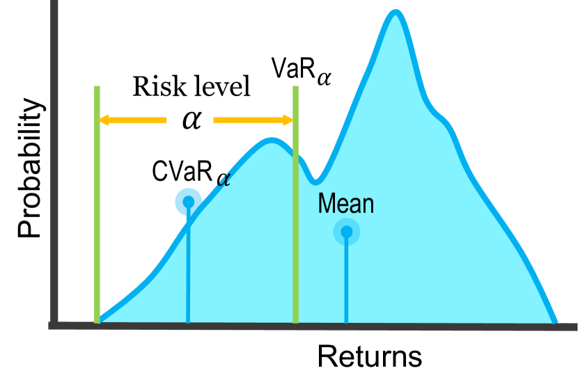
Figure 1: CVaR

CVaR (Figure 1) is the expectation of values that are less equal than the $\alpha$-percentile value of the distribution over returns. Formally, let $X\in\mathcal{X}$ be a bounded random variable with cumulative distribution function $F(x)=\mathscr{P}\left[X\leq x\right]$ and the inverse CDF is $F^{-1}(u)=\inf\{x:F(x)\geq u\}$. CVaR at level $\alpha\in(0,1]$ of a random variable $X$ is then defined as $\text{CVaR}_{\alpha}(X):=\sup_{\nu}\left\{\nu-\frac{1}{\alpha}\mathbb{E}[{(\nu-X)^{+}]}\right\}$ (Rockafellar et al., 2000) when $X$ is a discrete random variable. Correspondingly, $\text{CVaR}_{\alpha}(X)=\mathbb{E}_{X\sim F}\left[X|X\leq F^{-1}(\alpha)\right]$ (Acerbi & Tasche, 2002) when $X$ has a continuous distribution. The $\alpha$-percentile value is value at risk (VaR). For ease of notation, we write CVaR as $\text{CVaR}_{\alpha}(F)$.

Figure 2: Our framework (dotted arrow indicates that gradients are blocked during training). (a) Agent’s policy network. (b) The overall architecture (agent network and mixer). (c) Risk operator. Each agent $i$ applies an individual risk operator $\Pi_{\alpha_{i}}$ on its return distribution $Z_{i}(\cdot,\cdot)$ to calculate $C_{i}(\cdot,\cdot,\cdot)$ for execution given risk level $\alpha_{i}$ predicted by the dynamic risk level predictor $\psi_{i}$. $\{C_{i}(\cdot,\cdot,\cdot)\}_{i=1}^{N}$ are fed into the mixer for centralized training.

Risk-sensitive RL. Risk-sensitive RL uses risk criteria over policy/value, which is a sub-field of the Safety RL (García et al., 2015). Von Neumann & Morgenstern proposed the expected utility theory where a decision policy behaves as though it is maximizing the expected value of some utility functions. The condition is satisfied when the decision policy is consistent and has a particular set of four axioms. This is the most pervasive notion of risk-sensitivity. A policy maximizing a linear utility function is called risk-neutral, whereas concave or convex utility functions give rise to risk-averse or risk-seeking policies, respectively. Many measures are used in RL such as CVaR (Chow et al., 2015; Dabney et al., 2018a) and power formula (Dabney et al., 2018a). However, few works have been done in MARL and it cannot be easily extended. Our work fills this gap.

3 Methodology

3.1 CVaR of Return Distribution

In this section, we describe how we estimate the CVaR value. The value of CVaR can be either estimated through sampling or computed from the parameterized return distribution (Rockafellar & Uryasev, 2002). However, the sampling method is usually computationally expensive (Tang et al., 2020). Therefore, we let each agent learn a return distribution parameterized by a mixture of Dirac Delta ($\delta$) functions , which is demonstrated to be highly expressive and computationally efficient (Bellemare et al., 2017). For convenience, we provide the definition of the Generalized Return Probability Density Function (PDF).

Definition 1.

(Generalized Return PDF). For a discrete random variable $R\in\left[-R_{\operatorname{max}},R_{\operatorname{max}}\right]$ and probability mass function (PMF) $\mathscr{P}(R=r_{k})$, where $r_{k}\in\left[-R_{\operatorname{max}},R_{\operatorname{max}}\right]$, we define the generalized return PDF as: $f_{R}(r)=\sum\nolimits_{r_{k}\in R}\mathscr{P}_{R}(r_{k})\delta(r-r_{k})$. Note that for any $r_{k}\in R$, the probability of $R=r_{k}$ is given by the coefficient of the corresponding $\delta$ function, $\delta(r-r_{k})$.

We define the parameterized return distribution of each agent $i$ at time step $t$ as:

$$Z^{t}_{i}(\tau_{i},u^{t-1}_{i})=\sum\nolimits_{j=1}^{M}\mathscr{P}_{j}(\tau_{i},u^{t-1}_{i})\delta_{j}(\tau_{i},u^{t-1}_{i})$$ (1)

where $M$ is the number of Dirac Delta functions. $\delta_{j}(\tau_{i},u^{t-1}_{i})$ is the $j$-th Dirac Delta function and indicates the estimated value which can be parameterized by neural networks in practice. $\mathscr{P}_{j}(\tau_{i},u^{t-1}_{i})$ is the corresponding probability of the estimated value given local observations and actions. $\tau_{i}$ and $u^{t-1}_{i}$ are trajectories (up to that timestep) and actions of agent $i$, respectively. With the individual return distribution $Z^{t}_{i}(\tau_{i},u^{t-1}_{i})\in\mathcal{Z}$ and cumulative distribution function (CDF) $F_{Z_{i}(\tau_{i},u^{t-1}_{i})}$, we define the CVaR operator $\Pi_{\alpha_{i}}$, at a risk level $\alpha_{i}$ ($\alpha_{i}\in(0,1]$ and $i\in\mathcal{A}$), over return as $C^{t}_{i}(\tau_{i},u^{t-1}_{i},\alpha_{i})=\Pi_{\alpha^{t}_{i}}Z^{t}_{i}(\tau_{i},u^{t-1}_{i}):=\operatorname{CVaR}_{\alpha^{t}_{i}}(F_{Z^{t}_{i}(\tau_{i},u^{t-1}_{i})})$ where $C\in\mathcal{C}$. As we use CVaR on return distributions, it corresponds to risk-neutrality (expectation, $\alpha_{i}=1$) and indicates the improving degree of risk-aversion ($\alpha_{i}\rightarrow 0$). $\operatorname{CVaR}_{\alpha_{i}}$ can be estimated in a nonparametric way given ordering of Dirac Delta functions $\left\{\delta_{j}\right\}_{j=1}^{m}$ (Kolla et al., 2019) by leveraging the individual distribution:

$$\operatorname{CVaR}_{\alpha_{i}}=\sum\nolimits_{j=1}^{m}\mathscr{P}_{j}\delta_{j}\bm{1}\left\{\delta_{j}\leq\hat{v}_{m,\alpha_{i}}\right\},$$ (2)

where $\bm{1}\{\cdot\}$ is the indicator function and $\hat{v}_{m,\alpha_{i}}$ is estimated value at risk from $\hat{v}_{m,\alpha_{i}}=\lfloor\delta_{m(1-\alpha_{i})}\rfloor$ with $\lfloor\cdot\rfloor$ being floor function. This is a closed-form formulation and can be easily implemented in practice. The optimal action of agent $i$ can be calculated via $\arg\max_{u_{i}}C_{i}(\tau_{i},u^{t-1}_{i},\alpha_{i})$. We will introduce it in detail in Sec. 3.2.

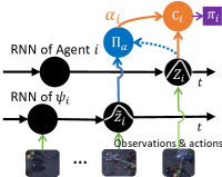
Figure 3: Agent architecture.

3.2 Risk Level Predictor

The values of risk levels, i.e., $\alpha_{i}$, $i\in\mathcal{A}$, are important for the agents to make decisions. Most of the previous works take a fixed value of risk level and do not take into account any temporal structure of agents’ trajectories, which is hard to tune the best risk level and may impede centralized training in the evolving multi-agent environments. Therefore, we propose the dynamic risk level predictor, which determines the risk levels of agents by explicitly taking into account the temporal nature of the stochastic outcomes, to alleviate time-consistency issue (Ruszczyński, 2010; Iancu et al., 2015) and stabilize the centralized training. Specifically, we represent the risk operator $\Pi_{\alpha}$ by a deep neural network, which calculates the CVaR value with predicted dynamic risk level $\alpha$ over the return distribution.

We show the architecture of agent $i$ in Figure 3 (agent network and risk operator with risk level predictor $\psi_{i}$, as shown in Figure 2) and illustrate how $\psi_{i}$ works with agent $i$ for CVaR calculation in practice in Figure 4. As depicted in Figure 4, at time step $t$, the agent’s return distribution is $Z_{i}$ and its historical return distribution is $\tilde{Z}_{i}$. Then we conduct the inner product to measure the discrepancy between the embedding of individual return distribution $f_{\operatorname{emb}}(Z_{i})$ and the embedding of past trajectory $\phi_{i}(\tau^{0:t-1}_{i},u^{t-1}_{i})$ modeled by GRU (Chung et al., 2014). We discretize the risk level range into $K$ even ranges for the purpose of computing. The $k$-th dynamic risk level $\alpha^{k}_{i}$ is output from $\psi_{i}$ and the probability of $\alpha^{k}_{i}$ is defined as:

$$\mathscr{P}(\alpha^{k}_{i})=\frac{\exp\left(\left<f_{\operatorname{emb}}(Z_{i})^{k},\phi_{i}^{k}\right>\right)}{\sum\nolimits_{k^{\prime}=0}^{K-1}\exp\left(\left<f_{\operatorname{emb}}(Z_{i})^{k^{\prime}},\phi_{i}^{k^{\prime}}\right>\right)}.$$ (3)

Then we get the $k\in[1,\dots,K]$ with the maximal probability by $\arg\max$ and normalize it into $(0,1]$, thus $\alpha_{i}=k/K$. The prediction risk level ${\alpha}_{i}$ is a scalar value and it is converted into a $K$-dimensional mask vector where the first $\lfloor\alpha_{i}\times K\rfloor$ items are one and the rest are zero. This mask vector is used to calculate the CVaR value (Eqn. 2) of each action-return distribution that contains $K$ Dirac functions. Finally, we obtain $C_{i}$ and the policy $\pi_{i}$ as illustrated in Figure 3. During training, $f_{\operatorname{emb}_{i}}$ updates its weights and the gradients of $f_{\operatorname{emb}_{i}}$ are blocked (the dotted arrow in Figure 3) in order to prevent changing the weights of the network of agent $i$.

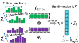
Figure 4: Risk level predictor $\psi_{i}$.

We note that the predictor differs from the attention network used in previous works (Iqbal & Sha, 2019; Yang et al., 2020) because the agent’s current return distribution and its return distribution of previous time step are separate inputs of their embeddings and there is no key, query and value weight matrices. The dynamic risk level predictors allow agents to determine the risk level dynamically based on historical return distributions and it is a hyperparameter (e.g., $\alpha$) tuning strategy as well.

3.3 Training

We train RMIX via addressing the two challenging issues: credit assignment and return distribution learning.

Loss Function. As there is only a global reward signal and agents have no access to individuals’ reward, we first utilize the monotonic mixing network ($f_{m}$) from QMIX to do Credit assignment. $f_{m}$ enforces a monotonicity constraint on the relationship between $C^{\operatorname{tot}}$ and each $C_{i}$ for RMIX:

$$\frac{\partial C^{\operatorname{tot}}}{\partial C_{i}}\geq 0,\forall i\in\{1,2,\ldots,N\},$$ (4)

where $C^{\operatorname{tot}}=f_{m}(C_{1}(\cdot,\cdot,\cdot),\cdots,C_{N}(\cdot,\cdot,\cdot))$ and $C_{i}(\tau_{i},u_{i},\alpha_{i})$ is the individual CVaR value of agent $i$. To ease the confusion, the $C^{\operatorname{tot}}$ is not the global CVaR value as modeling global return distribution as well as local distribution are challenging with the credit assignment issue in Dec-POMDP problems, and the risk level values are locally decided and used during training. Then, to maximize the CVaR value of each agent, we define the risk-sensitive Bellman operator $\mathcal{T}$:

$$\mathcal{T}C^{\operatorname{tot}}(\bm{s},\bm{u}):=\mathbb{E}\left[R(\bm{s},\bm{u})+\gamma\max_{\bm{u}^{\prime}}C^{\operatorname{tot}}(\bm{s}^{\prime},\bm{u}^{\prime})\right]$$ (5)

The risk-sensitive Bellman operator $\mathcal{T}$ operates on the $C^{\operatorname{tot}}$ and the reward, which can be proved to be a contracting operation, as shown in Proposition 1.

Proposition 1.

$\mathcal{T}:\mathcal{C}\mapsto\mathcal{C}$ is a $\gamma$-contraction.

Therefore, we can leverage the TD learning (Sutton & Barto, 2018) to train RMIX. Following the CTDE paradigm, we define our TD loss:

$$\mathcal{L}_{\Pi}(\theta):=\mathbb{E}_{\mathcal{D}^{\prime}\sim\mathcal{D}}\left[({y}_{t}^{\operatorname{tot}}-C^{\operatorname{tot}}\left(\bm{s}_{t},\bm{u}_{t}\right))^{2}\right]$$ (6)

where ${y}_{t}^{\operatorname{tot}}=\left(r_{t}+\gamma\max_{\bm{u}^{\prime}}C_{\bar{\theta}}^{\operatorname{tot}}\left(\bm{s}_{t+1},\bm{u}^{\prime}\right)\right)$, and $({y}_{t}^{\operatorname{tot}}-C_{\theta}^{\operatorname{tot}}\left(\bm{s}_{t},\bm{u}_{t}\right))$ is our CVaR TD error for updating CVaR values. $\theta$ is the parameters of $C^{\operatorname{tot}}$ which can be modeled by a deep neural network and $\bar{\theta}$ indicates the parameters of the target network which is periodically copied from $\theta$ for stabilizing training (Mnih et al., 2015). While training, gradients from $Z_{i}$ are blocked to avoid changing the weights of the agents’ network from the dynamic risk level predictor.

Local Return Distribution Learning. The CVaR estimation relies on accurately updating the local return distribution and the update is non-trivial. However, unlike many deep learning (Goodfellow et al., 2014) and distributional RL methods (Bellemare et al., 2017; Dabney et al., 2018b) where the label and local reward signal are accessible, in our problem, the exact rewards for each agent are unknown, which is very common in real world problems. To address this issue, we first consider CVaR values as dummy rewards of each agent due to its property of modeling the potential loss of return and then leverage the Quantile Regression (QR) loss used in Distributional RL (Dabney et al., 2018b) to explicitly update the local distribution decentrally. More concretely, QR aims to estimate the quantiles of the return distribution by minimizing the quantile regression loss between $Z_{i}(\tau_{i},u_{i})$ and its target distribution $\hat{Z}_{i}(\tau_{i},u_{i})=C_{i}(\tau_{i},u_{i},\alpha_{i})+\gamma Z_{i}({\tau_{i}}^{\prime},{u_{i}}^{\prime})$. Formally, the quantile distribution is represented by a set of quantiles $\tau_{j}=\frac{j}{K}$ and the quantile regression loss for Q network is defined as

$$\mathcal{L}_{QR}=\frac{1}{N}\sum\nolimits_{i=1}^{N}\sum\nolimits_{j=1}^{K}\mathbb{E}_{\hat{Z}_{i}\sim Z_{i}}[\rho_{\tau_{j}}(\hat{Z}_{i}-Z_{i})]$$ (7)

where $\rho_{\tau}(\nu)=\nu(\tau-\bm{1}\{\nu<0\})$. To eliminate cuspid in $\rho_{\tau}$ which could limit performance when using non-linear function approximation, quantile Huber loss is used as the loss function. The quantile Huber loss is defined as $\rho_{\tau}(\nu)=\mathcal{L}_{\kappa}(\nu)|\tau-\bm{1}\{\nu<0\}|$ where $\mathcal{L}_{\kappa}(\nu)$ is defined as:

$$\mathcal{L}_{\kappa}(\nu)=\begin{cases}\frac{1}{2}\nu^{2},&\text{if}|\nu|\geq\kappa,\\ \kappa(|\nu|-\frac{1}{2}\kappa),&\text{otherwise.}\end{cases}$$ (8)

Note that Risk-sensitive RL and Distributional RL are two orthogonal research directions as discussed in Sec. 1 and 2.

Training. Finally, we train RMIX in an end-to-end manner where each agent shares a single agent network and a risk predictor network to solve the lazy-agent issue (Sunehag et al., 2017). $\psi_{i}$ is trained together with the agent network via the loss defined in Eqn. 6. During training, $f_{\operatorname{emb}_{i}}$ updates its weights while the gradients of $f_{\operatorname{emb}_{i}}$ are blocked in order to prevent changing the weights of the return distribution in agent $i$. In fact, agents only use CVaR values for execution and the risk level predictor only predicts the $\alpha$; thus the increased network capacity is mainly from the local return distribution and the CVaR operator. Our framework is flexible and can be easily used in many cooperative MARL methods. We present our framework in Figure 2 and the pseudo code is shown in Appendix. All proofs are provided in Appendix.

Figure 5: Test Winning rates for six scenarios. More results can be found in Appendix.

4 Theoretical Analysis

Insightfully, our proposed method can be categorized into an overestimation reduction perspective which has been investigated in single-agent domain (Thrun & Schwartz, 1993; Hasselt, 2010; Lan et al., 2019; Chen et al., 2021). Intuitively, during minimizing $\mathcal{L}_{\Pi}(\theta)$ and policy execution, we can consider CVaR implementation as calculating the mean over k-minimum $\delta$ values of $Z_{i}$. It motivates us to analyse our method’s overestimation reduction property.

In single-agent cases, the overestimation bias occurs since the target $\max_{a^{\prime}}Q\left(s_{t+1},a^{\prime}\right)$ is used in the Q-learning update. This maximum operator over target estimations is likely to be skewed towards an overestimate as Q is an approximation which is possibly higher than the true value for one or more of the actions. In multi-agent scenarios, for example StarCraft II, the primary goal for each agent is to survive (maintain positive health values) and win the game. Overestimation on high return values might lead to agents suffering defeat early-on in the game.

Formally, in MARL, we characterize the relation between the estimation error, the in-target minimization parameter $\alpha$ and the number of Dirac functions, $M$, which consist of the return distribution. We follow the theoretical framework introduced in (Thrun & Schwartz, 1993) and extended in (Chen et al., 2021). More concretely, let $C^{\operatorname{tot}}(\bm{s},\bm{u})-Q(\bm{s},\bm{u})$ be the pre-update estimation bias for the output $C^{\operatorname{tot}}$ with the chosen individual CVaR values, where $Q(\bm{s},\bm{u})$ is the ground-truth Q-value. We are interested in how the bias changes after an update, and how this change is affected by risk level $\alpha$. The post-update estimation bias, which is the difference between two different targets, can be defined as:

$$\Psi_{\bm{\alpha}} \overset{\Delta}{=}r+\gamma\max_{\bm{u}^{\prime}}C^{\operatorname{tot}}\left(\bm{s}^{\prime},\bm{u}^{\prime}\right)-\left(r+\gamma\max_{\bm{u}^{\prime}}Q^{\operatorname{tot}}\left(\bm{s}^{\prime},\bm{u}^{\prime}\right)\right)$$

$$=\gamma\left(\max_{\bm{u}^{\prime}}C^{\operatorname{tot}}\left(\bm{s}^{\prime},\bm{u}^{\prime}\right)-\max_{\bm{u}^{\prime}}Q^{\operatorname{tot}}\left(\bm{s}^{\prime},\bm{u}^{\prime}\right)\right)$$

where $\bm{\alpha}=\{\alpha_{i}\}_{i=1}^{N}$ and $Q\left(\bm{s}^{\prime},\bm{u}^{\prime}\right)$ is output of the centralized mixing network with individuals’ $Q_{i}$ as input. Note that due to the zero-mean assumption, the expected pre-update estimation bias is $\mathbb{E}[C^{\operatorname{tot}}(\bm{s},\bm{u})-Q(\bm{s},\bm{u})]=0$ by following Thrun & Schwartz (1993) and Lan et al. (2019). Thus if $\mathbb{E}[\Psi_{\alpha}]>0$, the expected post-update bias is positive and there is a tendency for over-estimation accumulation; and if $\mathbb{E}[\Psi_{\alpha}]<0$, there is a tendency for under-estimation accumulation.

Theorem 1.

We summarize the following properties:
(1) Given $\bm{\alpha}_{1}$ and $\bm{\alpha}_{2}$ where $\alpha$ values in each set are identical, $\mathbb{E}[\Psi_{\bm{\alpha}_{1}}]\leq\mathbb{E}[\Psi_{\bm{\alpha}_{2}}]$ for $0<\alpha_{1}\leq\alpha_{2}\leq 1$, $\alpha_{1}\in\bm{\alpha}_{1}$ and $\alpha_{2}\in\bm{\alpha}_{2}$.
(2) $\exists\alpha_{i}\in(0,1]$ and $\bm{\alpha}=\{\alpha_{i}\}_{i=1}^{N}$, $\mathbb{E}[\Psi_{\bm{\alpha}}]<0$.

Theorem 1 implies that we can control the $\mathbb{E}[\Psi_{\bm{\alpha}}]$, bringing it from above zero (overestimation) to under zero (underestimation) by decreasing $\alpha$. Thus, we can control the post-update bias with the risk level $\alpha$ and boost the RMIX training on scenarios where overestimation can lead to failure of cooperation. In the next section, we will present the empirical results.

5 Experiments

We empirically evaluate our method on various StarCraft II (SCII) scenarios where agents coordinate and defeat the opponent. Especially, we are interested in the robust cooperation between agents and agents’ learned risk-sensitive policies in complex asymmetric and homogeneous/heterogeneous scenarios. Additional introduction of scenarios and results are in Appendix.

(a) 5m_vs_6m

(b) MMM2

Figure 6: SMAC scenarios: 5m_vs_6m and MMM2.

5.1 Experiment Setup

StarCraft II. We consider SMAC (Samvelyan et al., 2019) benchmark, a challenging set of cooperative SCII maps for micromanagement, as our evaluation environments. The version SCII simulator is 4.10. We evaluate our method for every 10,000 training steps during training by running 32 episodes in which agents trained with our method battle with built-in game bots. We report the mean test won rate (percentage of episodes won of MARL agents) along with one standard deviation of test won rate (shaded in figures). We present the results of our method and baselines on 6 scenarios: 1c3s5z, MMM2, 5m_vs_6m, 8m_vs_9m, 10m_vs_11m and corridor.

Table 1: Baselines

Baselines	Description
IQL	Tampuu et al. (2017)
VDN	Sunehag et al. (2017)
COMA	Foerster et al. (2017)
QMIX	Rashid et al. (2018)
QTRAN	Son et al. (2019)
MAVEN	Mahajan et al. (2019)
LH-IQN	Lyu & Amato (2020)
QR-MIX	Hu et al. (2020)
Qatten	Yang et al. (2020)

Baselines and training. We show baselines in Table 1. We implement our method on PyMARL (Samvelyan et al., 2019) and use 5 random seeds to train each method. We carry out experiments on NVIDIA Tesla V100 GPU 16G.

5.2 Experimental Results

5.2.1 Comparison with baseline methods

Comparison with value-based MARL baselines. As depicted in Figure 5, RMIX demonstrates substantial superiority over baselines in asymmetric and homogeneous scenarios. RMIX outperforms baselines in asymmetric homogeneous scenarios: 5m_vs_6m (super hard and asymmetric), 8m_vs_9m (easy and asymmetric), 10m_vs_11m (easy and asymmetric) and corridor (super hard and asymmetric). On 1c3s5z (easy and symmetric heterogeneous) and MMM2 (super hard and symmetric heterogeneous), RMIX also shows leading performance over baselines. RMIX improves coordination in a sample efficient way via risk-sensitive policies. Intuitively, for asymmetric scenarios, agents can be easily defeated by the opponents. As a consequence, coordination between agents is cautious in order to win the game, and the cooperative strategies in these scenarios should avoid massive casualties in the starting stage of the game. Apparently, our risk-sensitive policy representation works better than vanilla expected Q values (QMIX, VDN and IQL, et al.) in evaluation. In heterogeneous scenarios, action space and observation space are different among different types of agents, and methods with vanilla expected action value are inferior to RMIX.

Interestingly, as illustrated in Figure 7, RMIX also demonstrates leading exploration performance on super hard corridor scenario, where there is a narrow corridor connecting two separate rooms, and agents should learn to cooperatively combat the opponents to avoid being beaten by opponents with the divide-and-conquer strategy. RMIX outperforms MAVEN (Mahajan et al., 2019), which was originally proposed for tackling multi-agent exploration problems, both in sample efficiency and performance. After 5 million training steps, RMIX starts to converge while MAVEN starts to converge after over 7 million training steps.

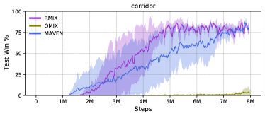
Figure 7: Test Winning rates for super hard scenario: corridor.

Comparison with Centralized Distributional MARL baseline. We compare RMIX with QR-MIX, which learns a centralized return distribution while the policies of each agent are conventional Q values. As shown in Figure 5, RMIX shows leading performance and superior sample efficiency over QR-MIX on 6 scenarios. With a centralized return distribution, QR-MIX presents slightly better performance over other baselines on 1c3s5z, MMM2 and 5m_vs_6m. The results show that learning individual return distributions can better capture the randomness and thus improve the overall performance compared with learning central distribution which is only used during training while the individual returns are expected Q values.

Comparison with risk-sensitive MARL baseline. Although there are few practical methods on risk-sensitive multi-agent reinforcement learning, we also conduct experiments to compare our method with LH-IQN (Lyu & Amato, 2020), which is a risk-sensitive method built on implicit Quantile network. We can find that our method outperforms LH-IQN in many scenarios. LH-IQN performs poorly on StarCraft II scenarios as it is an independent learning MARL methods like IQL.

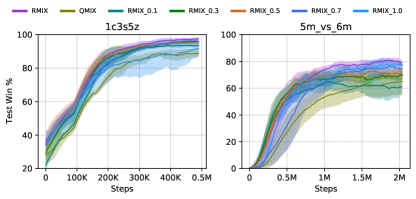
Figure 8: Ablation studies on various static risk levels.

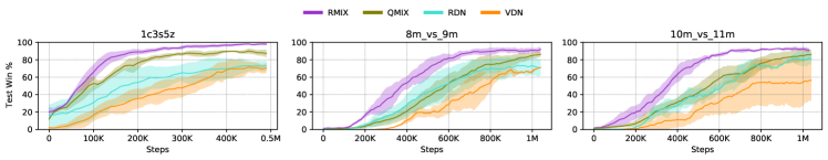
Figure 9: Test Winning rates of RMIX, RDN, VDN and QMIX.

Figure 10: Results analysis of RMIX on corridor. There are 8 scenes as examples. Further discussion can be found in Sec. 5.3.

5.2.2 Ablations

RMIX mainly consists of two components: the CVaR policies and the risk level predictor. The CVaR policies are different vanilla Q values and the risk level predictor is proposed to model the temporal structure and as an $\alpha$-finding strategy for hyperparameter tuning. Our ablation studies serve to answer the following questions: (a) Can RMIX with static $\alpha$ also work? (b) Can the risk level predictor learn $\alpha$ values and fast learn a good policy compared with RMIX with static $\alpha$? (c) Can our framework be applied to other methods?

To answer the above questions, we first conduct an ablation study by fixing the risk level in RMIX with the value of $\{0.1,0.3,0.5,0.7,1.0\}$ and compare with RMIX and QMIX on 1c3s5z (easy and symmetric heterogeneous) and 5m_vs_6m (super hard and asymmetric). As illustrated in Figure 8, with static $\alpha$ values, RMIX is capable of learning good performance over QMIX, which demonstrates the benefits of learning risk-sensitive MARL policies in complex scenarios where the potential of loss should be taken into consideration in coordination. With risk level predictor, RMIX converges faster than RMIX with static $\alpha$ values, illustrating that agents have captured the temporal features of scenarios and possessed the $\alpha$ value tuning merit.

To show that our proposed method is flexible in other mixing networks, we then apply additivity of individual CVaR values to represent the global CVaR value as $C^{\operatorname{tot}}(\bm{\tau},\bm{u})=C_{1}(\tau_{1},u_{1},\alpha_{1})+\cdots+C_{N}(\tau_{N},u_{N},\alpha_{N})$. Following the training of RMIX, we name this method Risk Decomposition Network (RDN). We use experiment setup of VDN and train RDN on 3 SMAC scenarios. With CVaR values of actions as policies, RDN outperforms VDN on 10m_vs_11m and converges faster than VDN on 1c3s5z and 8m_vs_9m, as depicted in Figure 9, demonstrating that our framework can be applied to VDN and outperforms VDN.

5.3 Results Analysis

We are interested in finding if the risk level predictor can predict temporal risk levels. We use the trained model of RMIX and run the model to collect one episode data including game replay, states, actions, rewards and $\alpha$ values. As shown in Figure 10, the first row shows the rewards of one episode and the second row shows the $\alpha$ value each agent predicts per time step. There are eight scenes in the third row to show how agents learn time-consistency $\alpha$ values. Scenes in Figure 10 are screenshots from the game replay.

We use trajectories of agent 0, 1 and 3 as examples in Figure 10. Number in the circle indicates the index of the agent. Scene (1): one episode starts, 6 Zealots consist of RMIX agents and 24 Zerglings compose enemies; Scene (2): in order to win the game, agent 3 draws the attention of enemies and goes to the other side of the battlefield. The $\alpha$ value is $0.3$ at step 2. Many enemies are chasing agent 3. The rest agents are combating with fewer number enemies; Scene (3): at step 14, agent 3 is at the corner of the battlefield the $\alpha$ is decreasing. As being outnumbered, agent 3 quickly dies and the $\alpha$ is zero; Scene (4) agent 0 and 1 show similar $\alpha$ values as they are walking around and fighting with enemies from time step 22 to 30. Then agents kill enemies around and planing to go to the other side of the battlefield in order to win the game; Scene (5): agent 0 (low health value) is walking through the corridor alone to draw enemies to come over. To avoid being killed, $\alpha$ values are low (step 46-50) which means the policy is risk-averse. From step 38 and step 51, reward is zero; Scene (6): agent 0 is facing many enemies and luckily its teammates are coming to help. So, the $\alpha$ is increasing (step 50); Scene (7): as there are many teammates around and the number of enemies is small, agents are going to win. Agent 0 and agent 1 walk outside the range of the observations of enemies in order to survive. The $\alpha$ values of agent 0 and agent 1 are 1 (risk-neutral); Scene (8): agents win the game. The video is available on this link: https://youtu.be/5yBEdYUhysw. Interestingly, the result shows emergent cooperation strategies between agents at different step during the episode, which demonstrates the superiority of RMIX.

6 Conclusion and Future Work

In this paper, we propose RMIX, a novel and practical MARL method with CVaR over the learned distributions of individuals’ Q values as risk-sensitive policies for cooperative agents. Empirically, we show that our method outperforms baseline methods on many challenging StarCraft II tasks, reaching the state-of-the-art performance and demonstrating significantly enhanced coordination as well as high sample efficiency.

Risk-sensitive policy learning is vital for many real-world multi-agent applications especially in risky tasks, for example autopilot vehicles, military action, resource allocation, finance portfolio management and Internet of Things (IoT). For the future work, better risk measurement together with accurate spatial-temporal trajectory representation can be investigated. Also, learning to model other agents’ risk levels and reach consensus with communication can be another direction for enhancing multi-agent coordination.

Appendix A Proofs

We present proofs of our propositions and theorem introduced in the main text. The numbers of proposition, theorem and equations are reused in restated propositions.

Assumption 1.

The mean rewards are bounded in a known interval, i.e., $r\in[-R_{\operatorname{max}},R_{\operatorname{max}}]$.

This assumption means we can bound the absolute value of the Q-values as $|Q_{sa}|\leq Q_{\operatorname{max}}=HR_{\operatorname{max}}$, where $H$ is the maximum time horizon length in episodic tasks.

See 1

Proof.

We consider the sup-norm contraction,

$$\left|\mathcal{T}C_{(1)}(\bm{s},\bm{u})-\mathcal{T}C_{(2)}(\bm{s},\bm{u})\right|\leq\gamma\left\lVert C_{(1)}(\bm{s},\bm{u})-C_{(2)}(\bm{s},\bm{u})\right\lVert_{\infty}\quad\forall\bm{s}\in\mathcal{S},\bm{u}\in\mathcal{U}.$$ (9)

The sup-norm is defined as $\left\lVert C\right\lVert_{\infty}=\sup_{\bm{s}\in\mathcal{S},\bm{u}\in\mathcal{U}}\left|C(\bm{s},\bm{u})\right|$ and $C\in\mathbb{R}$.

In $\{C_{i}\}^{N}_{i=1}$, the risk level is fixed and can be considered implicit input. Given two different return distributions $Z_{(1)}$ and $Z_{(2)}$, we prove:

$$\left|\mathcal{T}C_{(1)}-\mathcal{T}C_{(2)}\right| \leq\max_{\bm{s},\bm{u}}\left|\left[\mathcal{T}C_{(1)}\right](\bm{s},\bm{u})-\left[\mathcal{T}C_{(2)}\right](\bm{s},\bm{u})\right|$$ (10)

$$=\max_{\bm{s},\bm{u}}\left|\gamma\sum\nolimits_{\bm{s}^{\prime}}\mathcal{P}(\bm{s}^{\prime}|\bm{s},\bm{u})\left(\max_{\bm{u}^{\prime}}C_{(1)}(\bm{s}^{\prime},\bm{u}^{\prime})-\max_{\bm{u}^{\prime}}C_{(2)}(\bm{s}^{\prime},\bm{u}^{\prime})\right)\right|$$

$$\leq\gamma\max_{\bm{s}^{\prime}}\left|\max_{\bm{u}^{\prime}}C_{(1)}(\bm{s}^{\prime},\bm{u}^{\prime})-\max_{\bm{u}^{\prime}}C_{(2)}(\bm{s}^{\prime},\bm{u}^{\prime})\right|$$

$$\leq\gamma\max_{\bm{s}^{\prime},\bm{u}^{\prime}}\left\lvert C_{(1)}(\bm{s}^{\prime},\bm{u}^{\prime})-C_{(2)}(\bm{s}^{\prime},\bm{u}^{\prime})\right\lvert$$

$$=\gamma\left\lVert C_{(1)}-C_{(2)}\right\lVert_{\infty}$$

This further implies that

$$\left|\mathcal{T}C_{(1)}-\mathcal{T}C_{(2)}\right|\leq\gamma\left\lVert C_{(1)}-C_{(2)}\right\lVert_{\infty}\quad\forall\bm{s}\in\mathcal{S},\bm{u}\in\mathcal{U}.$$ (11)

∎

With proposition 1, we can leverage the TD learning (Sutton & Barto, 2018) to compute the maximal CVaR value of each agent, thus leading to the maximal global CVaR value.

Proposition 2.

For any agent $i\in\{1,\dots,N\}$, $\exists\lambda(\tau_{i},u_{i})\in\left(0,1\right]$, such that $C_{i}(\tau_{i},u^{t-1}_{i})=\lambda(\tau_{i},u^{t-1}_{i})\mathbb{E}\left[Z_{i}(\tau_{i},u^{t-1}_{i})\right]$.

Proof.

We first provide that given a return distribution $Z$, return random variable $\mathscr{Z}$ and risk level $\alpha\in\mathcal{A}$, $\forall z$, $\Pi_{\alpha}Z$ can be rewritten as $\mathbb{E}\left[\mathscr{Z}|\mathscr{Z}<z\right]<\mathbb{E}\left[\mathscr{Z}\right]$. This can be easily proved by following (Privault, 2020)’s proof. Thus we can get $\Pi_{\alpha}Z<\mathbb{E}\left[Z\right]$, and there exists $\lambda_{(\tau_{i},u^{t-1}_{i})}\in(0,1]$, which is a value of agent’s trajectories, such that $\Pi_{\alpha}Z_{i}(\tau_{i},u^{t-1}_{i})=\lambda_{(\tau_{i},u_{i})}\mathbb{E}\left[Z_{i}(\tau_{i},u^{t-1}_{i})\right]$. ∎

Proposition 2 implies that we can view the CVaR value as truncated values of Q values that are in the lower region of return distribution $Z_{i}(\tau_{i},u_{i})$. CVaR can be decomposed into two factors: $\lambda_{(\tau_{i},u_{i})}$ and $\mathbb{E}[Z_{i}(\tau_{i},u_{i})]$.

See 1

Proof.

We first consider the static risk level for each agent and the linear additivity mixer (Sunehag et al., 2017) of individual CVaR values.

(1) Given $\bm{\alpha}_{1}$ and $\bm{\alpha}_{2}$ and the mixer is the additivity function, we derive $\mathbb{E}[\Psi_{\alpha}]$ as follows

$$\mathbb{E}[\Psi_{\alpha}] \overset{\Delta}{=}\mathbb{E}\left[r+\gamma\max_{\bm{u}^{\prime}}C^{\operatorname{tot}}\left(\bm{s}^{\prime},\bm{u}^{\prime}\right)-\left(r+\gamma\max_{\bm{u}^{\prime}}Q\left(\bm{s}^{\prime},\bm{u}^{\prime}\right)\right)\right]$$ (12)

$$=\mathbb{E}\left[\gamma\left(\max_{\bm{u}^{\prime}}C^{\operatorname{tot}}\left(\bm{s}^{\prime},\bm{u}^{\prime}\right)-\max_{\bm{u}^{\prime}}Q\left(\bm{s}^{\prime},\bm{u}^{\prime}\right)\right)\right]$$ (13)

$$=\mathbb{E}\left[\gamma\left(\sum\nolimits_{i=1}^{N}\max_{u_{i}}C_{i}(\tau_{i},u^{t-1}_{i},\alpha)-\sum\nolimits_{i=1}^{N}\max_{u_{i}}Q_{i}(\tau_{i},u^{t-1}_{i})\right)\right]$$ (14)

Following Proposition 2 and Eqn. 2, given $\alpha_{1}\leq\alpha_{2}$ and for any $i\in N$ and $u\in\mathcal{U}$, we can easily derive

$$C_{i}(\tau_{i},u^{t-1}_{i},\alpha_{1})\leq C_{i}(\tau_{i},u^{t-1}_{i},\alpha_{2})$$ (15)

Thus,

$$\max_{u_{i}}C_{i}(\tau_{i},u^{t-1}_{i},\alpha_{1})\leq\max_{u_{i}}C_{i}(\tau_{i},u^{t-1}_{i},\alpha_{2})$$ (16)

Then, we can get

$$\mathbb{E}[\Psi_{\alpha_{1}}] =\mathbb{E}\left[\gamma\left(\sum\nolimits_{i=1}^{N}\max_{u_{i}}C_{i}(\tau_{i},u^{t-1}_{i},\alpha_{1})-\sum\nolimits_{i=1}^{N}\max_{u_{i}}Q_{i}(\tau_{i},u^{t-1}_{i})\right)\right]$$ (17)

$$\leq\mathbb{E}\left[\gamma\left(\sum\nolimits_{i=1}^{N}\max_{u_{i}}C_{i}(\tau_{i},u^{t-1}_{i},\alpha_{2})-\sum\nolimits_{i=1}^{N}\max_{u_{i}}Q_{i}(\tau_{i},u^{t-1}_{i})\right)\right]$$ (18)

$$=\mathbb{E}[\Psi_{\alpha_{2}}]$$ (19)

Finally, we get $\mathbb{E}[\Psi_{\alpha_{1}}]\leq\mathbb{E}[\Psi_{\alpha_{2}}]$.

Note that, it also applies when the mixer is the monotonic network by following the proof of Theorem 1 in (Rashid et al., 2020). Here we present the proof in RMIX for the convenience of readers.

With monotonicity network $f_{\operatorname{m}}$, in RMIX, we have

$$C^{\operatorname{tot}}(\bm{s},\bm{u})=f_{\operatorname{m}}(C_{1}(\tau_{1},u_{1},\alpha_{1}),\dots,C_{n}(\tau_{n},u_{n},\alpha_{n}))$$ (20)

Consequently, we have

$$C^{\operatorname{tot}}(\bm{s},\{\arg\max_{u^{\prime}}C_{i}(\tau_{i},u^{\prime},\alpha_{i})\}_{i=1}^{N})=f_{\operatorname{m}}(\{\max_{u^{\prime}}C_{i}(\tau_{i},u^{\prime},\alpha_{i})\}_{i=1}^{N})$$ (21)

By the monotonocity property of $f_{\operatorname{m}}$, we can easily derive that if $j\in\{1,\dots,N\}$, $u^{*}_{j}=\arg\max_{u_{i}}C_{j}(\tau_{j},u^{t-1}_{j},\alpha_{j})$, $\alpha_{j}\in(0,1]$ is the risk level given the current return distributions and historical return distributions, and actions of other agents are not the best action, then we have

$$f_{\operatorname{m}}(\{C_{j}(\tau_{j},u_{j},\alpha_{j})\}_{i=1}^{N})\leq f_{\operatorname{m}}(\{C_{j}(\tau_{j},u_{j},\alpha_{j})\}_{i=1,i\neq j}^{N},C_{j}(\tau_{j},u^{*}_{j},\alpha_{j})).$$ (22)

So, for all agents, $\forall j\in\{1,\dots,N\}$, $u^{*}_{j}=\arg\max_{u_{j}}C_{j}(\tau_{j},u^{t-1}_{j},\alpha_{j})$, we have

$$f_{\operatorname{m}}(\{C_{j}(\tau_{i},u_{i},\alpha_{i})\}_{i=1}^{N}) \leq f_{\operatorname{m}}(\{C_{j}(\tau_{j},u_{j},\alpha_{j})\}_{i=0,i\neq j}^{n-1},C_{j}(\tau_{j},u^{*}_{j}))$$ (23)

$$\leq f_{\operatorname{m}}(\{C_{i}(\tau_{i},u^{*}_{i},\alpha_{i})\}_{i=1}^{N})$$ (24)

$$=\max_{\{u_{i}\}_{i=1}^{N}}f_{\operatorname{m}}(\{C_{i}(\tau_{i},u_{i},\alpha_{i})\}_{i=1}^{N}).$$ (25)

Therefore, we can get

$$\max_{\{u_{i}\}_{i=1}^{N}}f_{\operatorname{m}}(\{C_{i}(\tau_{i},u_{i},\alpha_{i})\}_{i=1}^{N})=\max_{\bm{u}}C^{\operatorname{tot}}(\bm{s},\bm{u}),$$ (26)

which implies

$$\max_{\bm{u}}C^{\operatorname{tot}}(\bm{s},\bm{u})=C^{\operatorname{tot}}(\bm{s},\{\arg\max_{u^{\prime}}C_{i}(\tau_{i},u^{\prime})\}_{i=1}^{N}).$$ (27)

The Eqn. 26 can be used in Eqn. 13 to derive the about results.

(2) By following Proposition 2. We can get

$$\mathbb{E}[\Psi_{\bm{\alpha}}] =\mathbb{E}\left[\gamma\left(\sum\nolimits_{i=1}^{N}\max_{u_{i}}C_{i}(\tau_{i},u^{t-1}_{i},\alpha_{i})-\sum\nolimits_{i=1}^{N}\max_{u_{i}}Q_{i}(\tau_{i},u^{t-1}_{i})\right)\right]$$ (28)

$$=\mathbb{E}\left[\gamma\left(\sum\nolimits_{i=1}^{N}\max_{u_{i}}C_{i}(\tau_{i},u^{t-1}_{i},\alpha_{2})-\sum\nolimits_{i=1}^{N}\max_{u_{i}}Q_{i}(\tau_{i},u^{t-1}_{i})\right)\right]$$ (29)

$$=\mathbb{E}\left[\gamma\left(\sum\nolimits_{i=1}^{N}\max_{u_{i}}\lambda_{(\tau_{i},u^{t-1}_{i})}Q_{i}(\tau_{i},u^{t-1}_{i})-\sum\nolimits_{i=1}^{N}\max_{u_{i}}Q_{i}(\tau_{i},u^{t-1}_{i})\right)\right]$$ (30)

$$=\mathbb{E}\left[\gamma\left(\sum\nolimits_{i=1}^{N}\max_{u_{i}}\left((\lambda_{(\tau_{i},u^{t-1}_{i})}-1)Q_{i}(\tau_{i},u^{t-1}_{i})\right)\right)\right]$$ (31)

We can get that $\exists\alpha_{i}\in(0,1]$ and $i\in\{1,\dots,N\}$, $\mathbb{E}[\Psi_{\alpha}]<0$. ∎

Appendix B Pseudo Code of RMIX

0:  $K$, $\gamma$;

0:  Initialize parameters $\theta$ of the network of agent, risk operator and monotonic mixing network;

0:  Initialize parameters $\bar{\theta}$ of the target network of agent, risk operator and monotonic mixing network;

0:  Initialize replay buffer $\mathcal{D}$;

1:  for $e\in\{1,\dots,\text{MAX\_EPISODE}\}$ do

2:     Start a new episode;

3:     while EPISODE_IS_NOT_TEMINATED do

4:        Get the global state $\bm{s}^{t}$;

5:        for all agent $i\in\{1,\dots,N\}$ do

6:           Get observation $o^{t}_{i}$ from the environment;

7:           Get action of last step $u^{t-1}_{i}$ from the environment;

8:           Estimate the local return distribution $Z^{t}_{i}(o^{t}_{i},u^{t-1}_{i})$;

9:           Predict the risk level $\alpha_{i}$ (Eqn. 3);

10:           Calculate CVaR values $C_{i}^{t}\left(o^{t}_{i},u^{t-1}_{i},\alpha_{i}\right)$ (Eqn. 2);

11:           Get the action $u^{t}_{i}=\arg\max_{u^{t}}C_{i}^{t}\left(o^{t}_{i},u^{t-1}_{i},\alpha_{i}\right)$;

12:        end for

13:        Concatenate $u^{t}_{i}$, $i$ $\in$ $[1,..,N]$ into $\mathbf{u}_{t}$;

14:        Execute $\bm{u}^{t}_{i}$ into environment;

15:        Receive global reward $r^{t}$ and observe a new state $\bm{s}^{\prime}$;

16:        Store $(\bm{s}^{t},\{o^{t}_{i}\}_{i\in[1,...,N]},\bm{u}^{t},r^{t},\bm{s}^{\prime})$ in replay buffer $\mathcal{D}$;

17:        if UPDATE then

18:           Sample a min-batch $\mathcal{D}^{\prime}$ from replay buffer $\mathcal{D}$;

19:           For each sample in $\mathcal{D}^{\prime}$, calculate CVaR value $C_{i}$ by following steps in line 6-11;

20:           Concatenate CVaR values $\{[C^{1}_{1},\dots,C^{1}_{N}]_{1},\dots,[C^{|\mathcal{D}^{\prime}|}_{1},\dots,C^{|\mathcal{D}^{\prime}|}_{N}]_{|\mathcal{D}^{\prime}|}\}$;

21:           For each $[C^{j}_{1},\dots,C^{j}_{N}]_{0,j\in[1,\dots,|\mathcal{D}^{\prime}|]}$, calculate $C^{\operatorname{tot}}_{j}$ in the mixing network;

22:           Update $\theta$ by minimizing the TD loss (Eqn. 6);

23:           if UPDATE then

24:              Update the local return via QR loss (Eqn.7);

25:           end if

26:           Update $\bar{\theta}$: $\bar{\theta}\leftarrow\theta$;

27:        end if

28:     end while

29:  end for

Algorithm 1 RMIX

Appendix C SMAC Settings

SMAC benchmark is a challenging set of cooperative StarCraft II maps for micromanagement developed by (Samvelyan et al., 2019) built on DeepMind’s PySC2 (Vinyals et al., 2017). We introduce states and observations, action space and rewards of SMAC, and environmental settings of RMIX below.

States and Observations. At each time step, agents receive local observations within their field of view, which contains information (distance, relative x, relative y, health, shield, and unit type) about the map within a circular area for both allied and enemy units and makes the environment partially observable for each agent. The global state is composed of the joint observations, which could be used during training. All features, both in the global state and in individual observations of agents, are normalized by their maximum values.

Action Space. actions are in the discrete space. Agents are allowed to make move[direction], attack[enemy id], stop and no-op. The no-op action is only for dead agents and it is the only legal action for them. Agents can only move in four directions: north, south, east, or west. The shooting range is set to for all agents. Having a larger sight range than a shooting range allows agents to make use of the move commands before starting to fire. The automatical built-in behavior of agents is also disabled for training.

Rewards. At each time step, the agents receive a joint reward equal to the total damage dealt on the enemy agents. In addition, agents receive a bonus of 10 points after killing each opponent, and 200 points after killing all opponents for winning the battle. The rewards are scaled so that the maximum cumulative reward achievable in each scenario is around 20.

Environmental Settings of RMIX. The difficulty level of the built-in game AI we use in our experiments is level 7 (very difficult) by default as many previous works did (Rashid et al., 2018; Mahajan et al., 2019). The scenarios used in Section 5 are shown in Table 2. We present the table of all scenarios in SMAC in Table 2 and the corresponding memory usage for training each scenario in Table 3. The Ally Units are agents trained by MARL methods and Enemy Units are built-in game bots. For example, 5m_vs_6m indicates that the number of MARL agent is 5 while the number of the opponent is 6. The agent (unit) type is marine. This asymmetric setting is hard for MARL methods.

Table 2: SMAC Environments

Name	Ally Units	Enemy Units	Type
5m_vs_6m	5 Marines	6 Marines	homogeneous & asymmetric
8m_vs_9m	8 Marines	9 Marines	homogeneous & asymmetric
10m_vs_11m	10 Marines	11 Marines	homogeneous & asymmetric
MMM2	1 Medivac, 2 Marauders & 7 Marines	1 Medivac, 3 Marauders & 8 Marines	heterogeneous & asymmetric
1c3s5z	1 Colossi & 3 Stalkers & 5 Zealots	1 Colossi & 3 Stalkers & 5 Zealots	heterogeneous & symmetric
corridor	6 Zealots	24 Zerglings	micro-trick: wall off

Appendix D Training Details

The baselines are listed in table 4 as depicted below. To make a fair comparison, we use episode (single-process environment for training, compared with parallel) runner defined in PyMARL to run all methods. The evaluation interval is $10,000$ for all methods. We use uniform probability to estimate $Z_{i}(\cdot,\cdot)$ for each agent. We use the other hyper parameters used for training in the original papers of all baselines. The metrics are calculated with a moving window size of 5. Experiments are carried out on NVIDIA Tesla V100 GPU 16G. We also provide memory usage of baselines (given the current size of the replay buffer) for training each scenario of SCII domain in SMAC. We use the same neural network architecture of agent used by QMIX (Rashid et al., 2018). The trajectory embedding network $\phi_{i}$ is similar to the network of the agent. The last layer of the risk level predictor generates the local return distribution and shares the same weights with the last layer of the agent network.

The QR loss is minimized to periodically (empirically every 50 time steps) update the weights of the agent as simultaneously updating the local distribution and the whole network can impede training. The QR loss is used for updating the local distribution while the TD loss of centralized training is for the agent network weights learning and credit assignment. In the QR loss, the $C_{i}(\cdot,\cdot,\cdot)$ is considered as scalar value and gradients from $C_{i}(\cdot,\cdot,\cdot)$ are blocked. As the QR update relies on accurately estimation of the dummy reward $C_{i}$, we start to update $C_{i}$ when the test wining rate is over 35%, which means the agents have grasped some strategies to win the game.

Table 3: Memory usage (given the current size of the replay buffer) for the training of each method (exclude COMA, which is an on-policy method without using replay buffer) on scenarios of SCII domain in SMAC.

Scenario	Memory Usage (GB)
5m_vs_6m	3
8m_vs_9m	4.9
10m_vs_11m	7.1
1c3s5z	8.6
MMM2	10.8
corridor	14.4

Table 4: Baseline algorithms

Algorithms	Brief Description
IQL (Tampuu et al., 2017)	Independent Q-learning
VDN (Sunehag et al., 2017)	Value decomposition network
COMA (Foerster et al., 2017)	Counterfactual Actor-critic
QMIX (Rashid et al., 2018)	Monotonicity Value decomposition
QTRAN (Son et al., 2019)	Value decomposition with linear affine transform
MAVEN (Mahajan et al., 2019)	MARL with variational method for exploration
QR-MIX (Hu et al., 2020)	MARL with Centralized Distributional Q
LH-IQN (Lyu & Amato, 2020)	Likelihood Hysteretic with IQN (independent learning)
Qatten (Yang et al., 2020)	Multi-head Attention for the estimation of the $Q^{\operatorname{tot}}$

Table 5: Hyper-parameters

hyper-parameter	Value
Batch size	32
Replay memory size	5,000
RMIX Optimizer	Adam
Learning rate (lr)	5e-4
Critic lr	5e-4
RMSProp alpha	0.99
RMSProp epsilon	0.00001
Gradient norm clip	10
Action-selector	$\epsilon$-greedy
$\epsilon$-start	1.0
$\epsilon$-finish	0.05
$\epsilon$-anneal time	50,000 steps
Target update interval	200
Evaluation interval	10,000
M	35
K	10
Runner	episode
Discount factor ($\gamma$)	0.99
RNN hidden dim	64

Appendix E Additional Results

Addtional Results.

We show the test return value in Figure 11 and RMIX outperforms baseline methods as well. As shown in Figure 12, RDN shows convincing test return value over VDN on three scenarios.

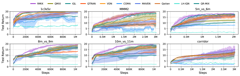
Figure 11: Test Return for six scenarios.

Figure 12: Test Return of RMIX, RDN, VDN, QMIX on three scenarios.

References

- Acerbi & Tasche (2002) Acerbi, C. and Tasche, D. On the coherence of expected shortfall. Journal of Banking & Finance, 26(7):1487–1503, 2002.
- Bellemare et al. (2017) Bellemare, M. G., Dabney, W., and Munos, R. A distributional perspective on reinforcement learning. In International Conference on Machine Learning, pp. 449–458, 2017.
- Chen et al. (2021) Chen, X., Wang, C., Zhou, Z., and Ross, K. W. Randomized ensembled double q-learning: Learning fast without a model. In International Conference on Learning Representations, 2021.
- Chow & Ghavamzadeh (2014) Chow, Y. and Ghavamzadeh, M. Algorithms for cvar optimization in MDPs. In Advances in Neural Information Processing Systems, pp. 3509–3517, 2014.
- Chow et al. (2015) Chow, Y., Tamar, A., Mannor, S., and Pavone, M. Risk-sensitive and robust decision-making: a cvar optimization approach. In Advances in Neural Information Processing Systems, pp. 1522–1530, 2015.
- Chung et al. (2014) Chung, J., Gulcehre, C., Cho, K., and Bengio, Y. Empirical evaluation of gated recurrent neural networks on sequence modeling. In Advances in Neural Information Processing Systems 2014 Workshop on Deep Learning, 2014.
- Dabney et al. (2018a) Dabney, W., Ostrovski, G., Silver, D., and Munos, R. Implicit quantile networks for distributional reinforcement learning. In International Conference on Machine Learning, pp. 1096–1105, 2018a.
- Dabney et al. (2018b) Dabney, W., Rowland, M., Bellemare, M. G., and Munos, R. Distributional reinforcement learning with quantile regression. In Proceedings of the AAAI Conference on Artificial Intelligence, pp. 2892–2901, 2018b.
- Foerster et al. (2017) Foerster, J., Farquhar, G., Afouras, T., Nardelli, N., and Whiteson, S. Counterfactual multi-agent policy gradients. arXiv preprint arXiv:1705.08926, 2017.
- García et al. (2015) García, J. et al. A comprehensive survey on safe reinforcement learning. Journal of Machine Learning Research, 16(42):1437–1480, 2015.
- Goodfellow et al. (2014) Goodfellow, I. J., Pouget-Abadie, J., Mirza, M., Xu, B., Warde-Farley, D., Ozair, S., Courville, A., and Bengio, Y. Generative adversarial nets. In Advances in Neural Information Processing Systems, pp. 2672–2680, 2014.
- Hasselt (2010) Hasselt, H. V. Double q-learning. In Advances in Neural Information Processing Systems, pp. 2613–2621, 2010.
- Hiraoka et al. (2019) Hiraoka, T., Imagawa, T., Mori, T., Onishi, T., and Tsuruoka, Y. Learning robust options by conditional value at risk optimization. In Advances in Neural Information Processing Systems, pp. 2619–2629, 2019.
- Hu et al. (2020) Hu, J., Harding, S. A., Wu, H., and Liao, S.-w. Qr-mix: Distributional value function factorisation for cooperative multi-agent reinforcement learning. arXiv preprint arXiv:2009.04197, 2020.
- Hüttenrauch et al. (2017) Hüttenrauch, M., Šošić, A., and Neumann, G. Guided deep reinforcement learning for swarm systems. In AAMAS 2017 Autonomous Robots and Multirobot Systems (ARMS) Workshop, 2017.
- Iancu et al. (2015) Iancu, D. A., Petrik, M., and Subramanian, D. Tight approximations of dynamic risk measures. Mathematics of Operations Research, 40(3):655–682, 2015.
- Iqbal & Sha (2019) Iqbal, S. and Sha, F. Actor-attention-critic for multi-agent reinforcement learning. In International Conference on Machine Learning, pp. 2961–2970, 2019.
- Keramati et al. (2020) Keramati, R., Dann, C., Tamkin, A., and Brunskill, E. Being optimistic to be conservative: Quickly learning a cvar policy. In Proceedings of the AAAI Conference on Artificial Intelligence, pp. 4436–4443, 2020.
- Kolla et al. (2019) Kolla, R. K., Prashanth, L., Bhat, S. P., and Jagannathan, K. Concentration bounds for empirical conditional value-at-risk: The unbounded case. Operations Research Letters, 47(1):16–20, 2019.
- Lan et al. (2019) Lan, Q., Pan, Y., Fyshe, A., and White, M. Maxmin q-learning: Controlling the estimation bias of q-learning. In International Conference on Learning Representations, 2019.
- Lillicrap et al. (2016) Lillicrap, T. P., Hunt, J. J., Pritzel, A., Heess, N., Erez, T., Tassa, Y., Silver, D., and Wierstra, D. Continuous control with deep reinforcement learning. In International Conference on Learning Representations, 2016.
- Lowe et al. (2017) Lowe, R., Wu, Y., Tamar, A., Harb, J., Abbeel, O. P., and Mordatch, I. Multi-agent actor-critic for mixed cooperative-competitive environments. In Advances in Neural Information Processing Systems, pp. 6379–6390, 2017.
- Lyu & Amato (2020) Lyu, X. and Amato, C. Likelihood quantile networks for coordinating multi-agent reinforcement learning. In Proceedings of the 19th International Conference on Autonomous Agents and MultiAgent Systems, pp. 798–806, 2020.
- Ma et al. (2020) Ma, X., Zhang, Q., Xia, L., Zhou, Z., Yang, J., and Zhao, Q. Distributional soft actor critic for risk sensitive learning. arXiv preprint arXiv:2004.14547, 2020.
- Mahajan et al. (2019) Mahajan, A., Rashid, T., Samvelyan, M., and Whiteson, S. MAVEN: Multi-agent variational exploration. In Advances in Neural Information Processing Systems, pp. 7613–7624, 2019.
- Majumdar & Pavone (2020) Majumdar, A. and Pavone, M. How should a robot assess risk? Towards an axiomatic theory of risk in robotics. In Robotics Research, pp. 75–84. Springer, 2020.
- Mnih et al. (2015) Mnih, V., Kavukcuoglu, K., Silver, D., Rusu, A. A., Veness, J., Bellemare, M. G., Graves, A., Riedmiller, M., Fidjeland, A. K., Ostrovski, G., et al. Human-level control through deep reinforcement learning. Nature, 518(7540):529–533, 2015.
- Oliehoek et al. (2008) Oliehoek, F. A., Spaan, M. T., and Vlassis, N. Optimal and approximate q-value functions for decentralized POMDPs. Journal of Artificial Intelligence Research, 32:289–353, 2008.
- Oliehoek et al. (2016) Oliehoek, F. A., Amato, C., et al. A Concise Introduction to Decentralized POMDPs, volume 1. Springer, 2016.
- Privault (2020) Privault, N. Notes on Financial Risk and Analytics. Course notes, 268 pages, 2020. Accessed: 2020-09-27.
- Rashid et al. (2018) Rashid, T., Samvelyan, M., Schroeder, C., Farquhar, G., Foerster, J., and Whiteson, S. QMIX: Monotonic value function factorisation for deep multi-agent reinforcement learning. In International Conference on Machine Learning, pp. 4295–4304, 2018.
- Rashid et al. (2020) Rashid, T., Samvelyan, M., De Witt, C. S., Farquhar, G., Foerster, J., and Whiteson, S. Monotonic value function factorisation for deep multi-agent reinforcement learning. Journal of Machine Learning Research, 21(178):1–51, 2020.
- Rockafellar & Uryasev (2002) Rockafellar, R. T. and Uryasev, S. Conditional value-at-risk for general loss distributions. Journal of Banking & Finance, 26(7):1443–1471, 2002.
- Rockafellar et al. (2000) Rockafellar, R. T., Uryasev, S., et al. Optimization of conditional value-at-risk. Journal of Risk, 2:21–42, 2000.
- Ruszczyński (2010) Ruszczyński, A. Risk-averse dynamic programming for markov decision processes. Mathematical Programming, 125(2):235–261, 2010.
- Samvelyan et al. (2019) Samvelyan, M., Rashid, T., de Witt, C. S., Farquhar, G., Nardelli, N., Rudner, T. G. J., Hung, C.-M., Torr, P. H. S., Foerster, J., and Whiteson, S. The StarCraft Multi-Agent Challenge. CoRR, abs/1902.04043, 2019.
- Silver et al. (2017) Silver, D., Schrittwieser, J., Simonyan, K., Antonoglou, I., Huang, A., Guez, A., Hubert, T., Baker, L., Lai, M., Bolton, A., et al. Mastering the game of Go without human knowledge. Nature, 550(7676):354–359, 2017.
- Singh et al. (2020) Singh, A. J., Kumar, A., and Lau, H. C. Hierarchical multiagent reinforcement learning for maritime traffic management. In Proceedings of the 19th International Conference on Autonomous Agents and MultiAgent Systems, pp. 1278–1286, 2020.
- Son et al. (2019) Son, K., Kim, D., Kang, W. J., Hostallero, D. E., and Yi, Y. QTRAN: Learning to factorize with transformation for cooperative multi-agent reinforcement learning. In International Conference on Machine Learning, pp. 5887–5896, 2019.
- Sunehag et al. (2017) Sunehag, P., Lever, G., Gruslys, A., Czarnecki, W. M., Zambaldi, V., Jaderberg, M., Lanctot, M., Sonnerat, N., Leibo, J. Z., Tuyls, K., et al. Value-decomposition networks for cooperative multi-agent learning. arXiv preprint arXiv:1706.05296, 2017.
- Sutton & Barto (2018) Sutton, R. S. and Barto, A. G. Reinforcement Learning: An Introduction. MIT press, 2018.
- Tamar et al. (2015) Tamar, A., Chow, Y., Ghavamzadeh, M., and Mannor, S. Policy gradient for coherent risk measures. In Advances in Neural Information Processing Systems, pp. 1468–1476, 2015.
- Tampuu et al. (2017) Tampuu, A., Matiisen, T., Kodelja, D., Kuzovkin, I., Korjus, K., Aru, J., Aru, J., and Vicente, R. Multiagent cooperation and competition with deep reinforcement learning. PLoS ONE, 12(4), 2017.
- Tang et al. (2020) Tang, Y. C., Zhang, J., and Salakhutdinov, R. Worst cases policy gradients. In Conference on Robot Learning, pp. 1078–1093, 2020.
- Thrun & Schwartz (1993) Thrun, S. and Schwartz, A. Issues in using function approximation for reinforcement learning. In Proceedings of the Fourth Connectionist Models Summer School, pp. 255–263, 1993.
- Vinyals et al. (2017) Vinyals, O., Ewalds, T., Bartunov, S., Georgiev, P., Vezhnevets, A. S., Yeo, M., Makhzani, A., Küttler, H., Agapiou, J., Schrittwieser, J., et al. StarCraft II: A new challenge for reinforcement learning. arXiv preprint arXiv:1708.04782, 2017.
- Vinyals et al. (2019) Vinyals, O., Babuschkin, I., Czarnecki, W. M., Mathieu, M., Dudzik, A., Chung, J., Choi, D. H., Powell, R., Ewalds, T., Georgiev, P., et al. Grandmaster level in StarCraft II using multi-agent reinforcement learning. Nature, 575(7782):350–354, 2019.
- Von Neumann & Morgenstern (1947) Von Neumann, J. and Morgenstern, O. Theory of Games and Economic Behavior, 2nd rev. Princeton university press, 1947.
- Yang et al. (2020) Yang, Y., Hao, J., Liao, B., Shao, K., Chen, G., Liu, W., and Tang, H. Qatten: A general framework for cooperative multiagent reinforcement learning. arXiv preprint arXiv:2002.03939, 2020.
- Zhang et al. (2020) Zhang, J., Bedi, A. S., Wang, M., and Koppel, A. Cautious reinforcement learning via distributional risk in the dual domain. arXiv preprint arXiv:2002.12475, 2020.