Practical application of the multi-model approach in the study of complex systems

Abstract

Different kinds of models are used to study various natural and technical phenomena. Usually, the researcher is limited to using a certain kind of model approach, not using others (or even not realizing the existence of other model approaches). The authors believe that a complete study of a certain phenomenon should cover several model approaches. The paper describes several model approaches which we used in the study of the random early detection algorithm for active queue management. Both the model approaches themselves and their implementation and the results obtained are described.

I Introduction

Scientific research is easy to start but difficult to complete. Our study of the Random Early Detection (RED) algorithm stood out from the study of approaches and mechanisms of traffic control in data transmission networks. But the further we went, the less satisfied we were with the results. The originally constructed mathematical model seemed to us somewhat artificial and non-extensible. To build a more natural mathematical model from first principles, we have developed a method of stochastization of one-step processes. To verify the mathematical model, we have built physical and simulation models. To conduct optimization studies, we began to build a surrogate model for the RED algorithm. At the last we came to an understanding that all of our models form some kind of emergent structure, with the help of which we can investigate various phenomena — stochastic and statistical systems in particular.

In this paper, we try to present our understanding of the multi-model approach to modeling.

II Model approaches

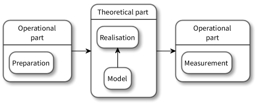
Modeling as a discipline encompasses different types of model approaches. From our point of view, these approaches can be schematically described in a unified manner (see Fig. 1). In this case, the research structure consists of operational and theoretical parts. The operational parts are represented by procedures of the system preparation and measurement. It is also common to describe the operational part as input and output data.

The theoretical part consists of two layers: a model layer and an implementation layer. The implementation layer describes the specific structure of the evolution of the system. Depending on the type of implementation, different types of models can be obtained: a mathematical model (implementation — mathematical expressions), a simulation model (implementation — an algorithm), a physical model (implementation — an analog system), a surrogate model (implementation — approximation of behavior). Each type of model has its area of applicability, its advantages and disadvantages. The use of the entire range of models allows the most in-depth and comprehensive study of the modeled system.

Figure 1: Generic structure of the model approach

III RED active queue management algorithm

Random Early Detection (RED) algorithm is at the heart of several mechanisms to prevent and control congestion in router queues. Its main purpose is to smooth out temporary bursts of traffic and prevent prolonged network congestion by notifying traffic sources about the need to reduce the intensity of information transmission.

The operation of a module implementing a RED-type algorithm can be schematically represented as follows.

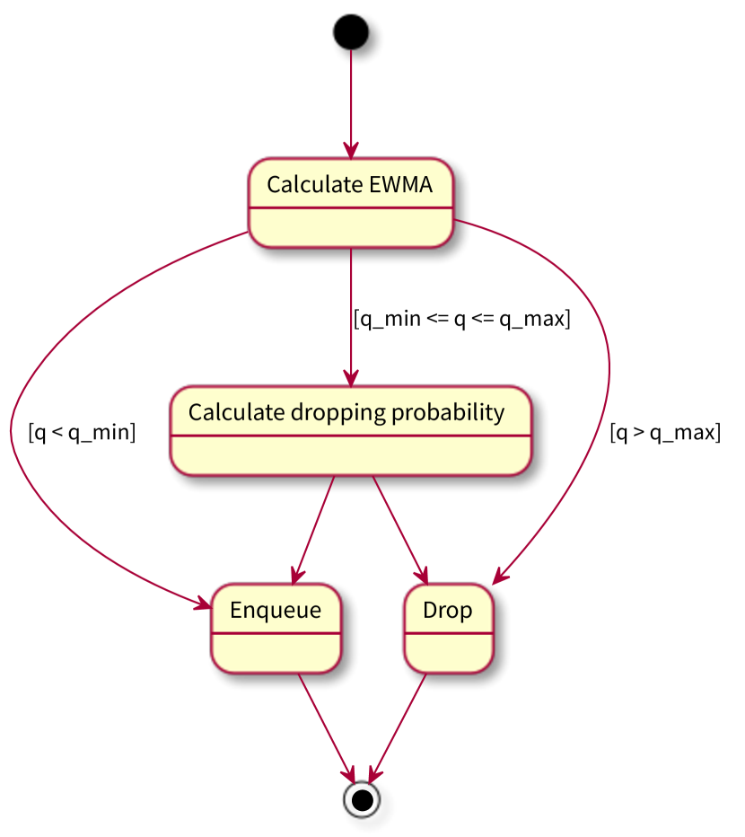
When a packet of transmitted data enters the system, it enters the reset module. The decision to remove the package is made based on the value of the $p(\hat{q})$ function received from the control unit. The function $p(\hat{q})$ depends on the exponentially weighted moving average of the queue length $\hat{q}$, also calculated by the ontrol unit based on the current value of the queue length $q$.

The classic RED algorithm is discussed in detail in floyd:1993:red . Only the formulas for calculating the reset function $p(\hat{q})$ and the exponentially weighted moving average queue length $\hat{q}$ are given here. The use of $\hat{q}$ is associated with the need to smooth outliers of the instantaneous queue length $q$.

To calculate $\hat{q}$, the recurrent formula for exponentially weighted moving average (EWMA) is used:

$$\hat{q}_{k+1}=(1-w_{q})\hat{q}_{k}+w_{q}q_{k},\quad k=0,1,2,\ldots,$$ (1)

where $w_{q}$, $0<w_{q}<1$ is the weight coefficient of the exponentially weighted moving average:

$$w_{q}=1-e^{-1/C},$$ (2)

where $C$ is the channel bandwidth (packets per second).

The $p(\hat{q})$ packet discard function linearly depends on the $\hat{q}$, the minimum $q_{\min}$ and maximum $q_{\max}$ thresholds and the maximum discard parameter $p_{\max}$, which sets the maximum packet discard level when $\hat{q}$ reaches the value $q_{\max}$, and the function $p(\hat{q})$ is calculated as follows:

$$p(\hat{q})=\begin{dcases}0,&0<\hat{q}\leqslant q_{\min},\\ \frac{\hat{q}-q_{\min}}{q_{\max}-q_{\min}}p_{\max},&q_{\min}<\hat{q}\leqslant q_{\max},\\ 1,&\hat{q}>q_{\max}.\end{dcases}$$ (3)

The drop function (3) describes the classic RED algorithm. And the main effort in the design of new algorithms like RED is directed at various modifications of the type of the drop function.

Since the complete simulated system consists of interoperable TCP and RED algorithms, it is necessary to simulate the evolution of the TCP source as well. Since the original model was based on the TCP Reno protocol, we simulated this particular protocol.

TCP uses a sliding window mechanism to deal with congestion. The implementation of this mechanism depends on the specific TCP protocol standard.

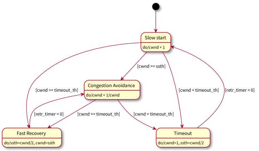
In TCP Reno the congestion control mechanism consists of the following phases: slow start, congestion avoidance, fast transmission, and fast recovery. The dynamics of the congestion window (CWND) size depends on the specific phase.

TCP Reno monitors two types of packet loss:

• Triple Duplicate ACK (TD). Let the $n$-th packet not to be delivered, and the subsequent packets ($n+1$, $n+2$, etc.) are delivered. For each packet delivered out of order (for $n+1$, $n+2$, etc.), the receiver sends an ACK message for the last undelivered ($n$-th) packet. Upon receipt of three such packets, the source resends the $n$-th packet. Besides, the window size is reduced by 2 times $cwnd\to cwnd/2$.

• Timeout (TO). When a packet is sent, the timeout timer is started. Each time a confirmation is received, the timer is restarted. The window is then set to the initial value of the overload window. The first lost packet is resent. The protocol enters the slow start phase.

The general congestion control algorithm is of the AIMD type (Additive Increase, Multiplicative Decrease) — an additive increase of the window size and its multiplicative decrease.

IV Mathematical model

Figure 2: Generic structure of the mathematical model

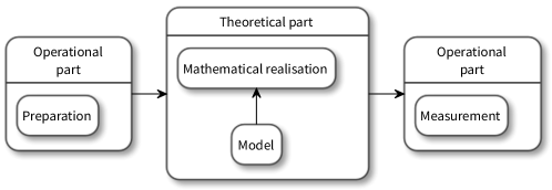
The most rigorous research is usually based on a mathematical model (see Fig. 2). In this case, the model layer is realized through mathematical expressions describing the evolution of the system.

There are several approaches to modeling RED-type algorithms. The most famous approach is modeling using the automatic control theory approach misra:1999:sdu ; misra:2000:fluid-based ; hollot:2001:control . To us, this approach seems somewhat artificial and inconsistent. We prefer to do our modeling from first principles.

We have developed a method of stochastization of one-step processes, which allows us to obtain models from first principles. Moreover, the resulting model models are immanently stochastic kulyabov:2018:pcs:stochastization_computer_algebra::en ; kulyabov:2016:mmcp:one-step ; kulyabov:2016:ecms:one-step . Our model of interaction between the TCP source and the RED algorithm is based on these methods and is mathematically represented in the form of stochastic differential equations with Wiener and Poisson processes kulyabov:2019:ecms:red-control ; kulyabov:2017:iopconf:self-oscillations ; kulyabov:2014:vestnik:red-sdu::en .

We will use the following notation. $W(t)$ is the TCP Reno window size, $Q(t)$ is the queue size, $T:=T(Q(t))$ is the round-trip time (taking into account equipment delays), $t$ is the time, $C$ is the queue service intensity, $\hat{Q}(t)$ is the Exponentially Weighted Moving-Average (EWMA) floyd:1993:red :

$$\hat{Q}(t)=(1-w_{q})\hat{Q}(t)+w_{q}Q(t),$$ (4)

where $w_{q}$, $0<w_{q}<1$ is the weight coefficient.

We used the method of stochastization of one-step processes to obtain the Fokker–Planck and Langevin equations for the stochastic processes $W(t)$ and $Q(t)$.

The kinetic equations will be:

$$\begin{dcases}0\xrightarrow{\frac{1}{W(t)}}W(t),\\ W(t)\xrightarrow{\frac{1}{2}\frac{\differential N(t)}{\differential t}}0,\\ 0\xrightarrow{\frac{W(t)}{T}}Q(t),\\ 0\xrightarrow{-C}Q(t),\end{dcases}$$ (5)

where $\differential N(t)$ is the Poisson process misra:2000:fluid-based .

Let us write down the Fokker–Planck equations corresponding to the kinetic equations (5):

$$\begin{gathered}\begin{multlined}\frac{\partial w(t)}{\partial t}=-\frac{\partial}{\partial W(t)}\left[\left(\frac{1}{W(t)}-\frac{W(t)}{2}\frac{\differential N(t)}{\differential t}\right)w(t)\right]+{}\\ {}+\frac{1}{2}\frac{\partial^{2}}{\partial W^{2}(t)}\left[\left(\frac{1}{W(t)}+\frac{W(t)}{2}\frac{\differential N(t)}{\differential t}\right)w(t)\right],\end{multlined}\frac{\partial w(t)}{\partial t}=-\frac{\partial}{\partial W(t)}\left[\left(\frac{1}{W(t)}-\frac{W(t)}{2}\frac{\differential N(t)}{\differential t}\right)w(t)\right]+{}\\ {}+\frac{1}{2}\frac{\partial^{2}}{\partial W^{2}(t)}\left[\left(\frac{1}{W(t)}+\frac{W(t)}{2}\frac{\differential N(t)}{\differential t}\right)w(t)\right],\\ \begin{multlined}\frac{\partial q(t)}{\partial t}=-\frac{\partial}{\partial Q(t)}\left[\left(\frac{W(t)}{T}-C\right)q(t)\right]+{}\\ {}+\frac{1}{2}\frac{\partial^{2}}{\partial Q^{2}(t)}\left[\left(\frac{W(t)}{T}-C\right)q(t)\right],\end{multlined}\frac{\partial q(t)}{\partial t}=-\frac{\partial}{\partial Q(t)}\left[\left(\frac{W(t)}{T}-C\right)q(t)\right]+{}\\ {}+\frac{1}{2}\frac{\partial^{2}}{\partial Q^{2}(t)}\left[\left(\frac{W(t)}{T}-C\right)q(t)\right],\end{gathered}$$ (6)

where $w(t)$ is the density of the random process $W(t)$, $q(t)$ is the density of the random process $Q(t)$.

The Langevin equations corresponding to the equations (6) have the form:

$$\begin{dcases}\differential W(t)=\frac{1}{T}\differential t-\frac{W(t)}{2}\differential N(t)+\sqrt{\frac{1}{T}+\frac{W(t)}{2}\frac{\differential N(t)}{\differential t}}\differential V^{1}(t),\\ \differential Q(t)=\left(\frac{W(t)}{T}-C\right)\differential Q(t)+\sqrt{\frac{W(t)}{T}-C}\differential V^{2}(t),\end{dcases}$$ (7)

where $\differential V^{1}(t)$ is the Wiener process corresponding to the random process $W(t)$, $\differential V^{2}(t)$ is the Wiener process corresponding to the random process $Q(t)$.

The equations (7) are supplemented by the constraint equation (written in differential form for convenience):

$$\frac{\differential\hat{Q}(t)}{\differential t}=w_{q}C(Q(t)-\hat{Q}(t)).$$ (8)

This mathematical model can be investigated both in the form of stochastic differential equations and by writing them down in moments. The equation in moments is naturally easier to study.

V Physical model

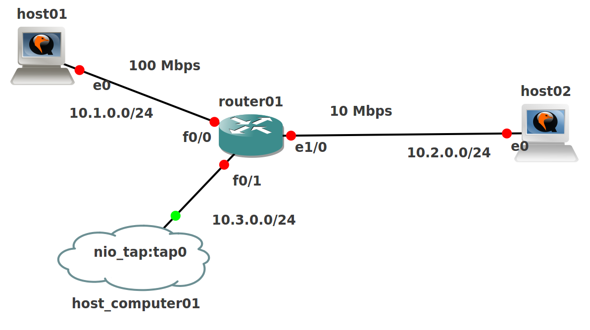
The resulting mathematical model should be compared with experimental data and verified. Unfortunately, we do not have the resources to take data from a working network or build a full-scale test bench on real network equipment. Therefore, we tried to create a virtual experimental installation based on the virtual machines kulyabov:2014:icumt-2014:gns3 . Virtual machines run images of real routers operating systems. This is what allows us to call this model physical.

To create the stand, the software package GNS3 (Graphical Network Simulator) welsh:2013:gns3 was chosen. This allows you to simulate a virtual network of routers and virtual machines. The software package GNS3 works on almost all platforms. It can be considered as a graphical interface for different virtual machines. To emulate Cisco devices the Dynamips emulator is used. Alternatively, emulators such as VirtualBox and Qemu can be used. The latter is especially useful when it used with a KVM system which allows a hardware processor implementation. GNS3 coordinates the operation of various virtual machines and also provides the researcher with a convenient interface for creation and customization of the required stand configuration. Also, the developed topology can be linked to an external network to manage and control data packets.

The stand consists of a Cisco router, a traffic generator, and a receiver. D-ITG (Distributed Internet Traffic Generator) is used as a traffic generator (see Fig. 3). D-ITG allows us to obtain estimates of the main indicators of the quality of service (average packet transmission delay, delay variation (jitter), packet loss rate, performance) with a high degree of confidence.

Figure 3: Virtual stand for studying the functioning of the RED algorithm. host01 is the packet source; host02 is the recipient.

VI Simulation model

With the development of computer technology it became possible to specify a model implementation not in the form of a mathematical description, but in the form of some algorithm (Fig. 4). This type of model is called simulation models and the approach itself is called simulation.

Figure 4: Generic structure of the simulation model

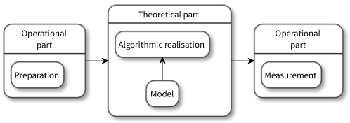
The simulation model plays a dual role. The simulation model, debugged and tested on experimental data and a physical model, can itself serve the purposes of the mathematical model verification. On the other hand, the simulation model makes it possible to study the behavior of the modeled system more effectively than the mathematical model for different variants of the input data.

VI.1 Simulation model on NS-2

The ns2 issariyakul:2012 ; altman:2011 package is the network protocol simulation tool. During its existence, the functionality has been repeatedly verified by data from field experiments. Therefore, this package itself has become a reference modeling tool. This is exactly the case when a simulation model is a replacement for a physical model and a natural experiment.

The program for ns2 is written in the TCL language welch:book:practical-tc-tk ; nadkarni:book:tcl-comprehensive . The simulation results can be represented using visualization tool nam (see Fig. 5).

The simulator is built on an event-driven architecture. That is, it implements a discrete approach to modeling. On the one hand, this is a plus, since it directly implements the TCP and RED specification (see section III). On the other hand, the amount of resulting data sharply increases, which makes it difficult to carry out any lengthy simulation experiment.

Figure 5: Visualization of the simulation. Packets drop is shown

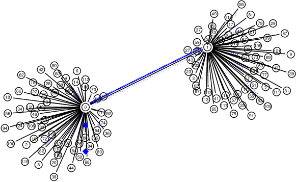
In our works, this software is used precisely for verification of the obtained results kulyabov:2018:icumt:aqm ; kulyabov:2019:aisc:self-oscillation .

VI.2 Hybrid model for RED algorithm

To study the RED algorithm we developed the prototype of the simulation model. We wanted to avoid the resource intensiveness of discrete modeling approaches. However, it was necessary to take into account the discrete specifics of TCP and RED (see section III). Therefore, we have chosen a hybrid (continuous–discrete) approach. The model was implemented in the hybrid modeling language Modelica fritzson:2003 ; fritzson:2011 .

Since we are building the hybrid continuous–discrete model, then to describe each phase of TCP functioning, we will turn to the model with continuous time. The transition between phases will be described by discrete states.

To build a hybrid model, we need:

• write a dynamic model for each state;

• replace systems with piecewise constant parameters with systems with variable initial conditions;

• write the state diagram of the model (Fig. 7 and 7).

The resulting diagrams are directly converted into a Modelica program kulyabov:2017:iop:tcp-modelica ; kulyabov:2019:ceur-ws:2407:red ; kulyabov:2016:ecms:red .

Figure 6: TCP state diagram

Figure 7: RED state diagram

VII Surrogate model

Figure 8: Generic structure of the surrogate model

Most scientific and technical problems require experiments and simulations to obtain results, to determine the limitations imposed on the result. However, for many real-world problems simulation alone can take minutes, hours, days. As a result, routine tasks such as decision optimization, decision space exploration, sensitivity analysis, and what-if analysis become impossible as they require thousands or millions of modeling evaluations.

One way to simplify research is to build surrogate models (approximation models, response surface models, metamodels, black box models) (see Fig. 8) that mimic the behavior of the original model so closely as much as possible, while being computationally cheap jin:2011:surrogate-assisted-computation . Surrogate models are built using a data-driven approach. The exact inner workings of the simulation code are not supposed to be known (or even understood), only the input—output (preparation—measurement) behavior is important. The model is built based on modeling the response to a limited number (sometimes quite large) of selected data points .

The scientific challenge for surrogate modeling is to create a surrogate that is as accurate as possible using as few modeling estimates as possible. The process consists of the following main stages kulyabov:2019:ceur-ws:2507:deep-learning :

• sample selection;

• construction of the surrogate model and optimization of model parameters;

• an estimate of the accuracy of the surrogate.

For some problems the nature of the true function is a priori unknown, so it is unclear which surrogate model will be the most accurate. Moreover, it is not clear how to obtain the most reliable estimates of the accuracy of a given surrogate. In this case, the model layer (Fig. 8) is replaced by the researcher’s guess. In our case, the surrogate model is based on a clearly formulated mathematical model, which allows us to obtain clear, substantiated results of surrogate modeling.

At this moment we are developing a methodology for constructing surrogate models for both RED type algorithms and arbitrary stochastic one-step processes.

VIII Conclusion

The authors tried to outline the concept of a multi-model approach to the study of physical and technical systems using the example of the interaction between the TCP protocol and the RED-type active queue management algorithm. This research is in line with the research of stochastic models in science and technology.

The multi-model approach makes it possible to increase the efficiency of the study of the phenomenon, to consider it from different angles, and to create effective software systems.