Hough²Map – Iterative Event-based Hough Transform for High-Speed Railway Mapping

Abstract

To cope with the growing demand for transportation on the railway system, accurate, robust, and high-frequency positioning is required to enable a safe and efficient utilization of the existing railway infrastructure. As a basis for a localization system we propose a complete on-board mapping pipeline able to map robust meaningful landmarks, such as poles from power lines, in the vicinity of the vehicle. Such poles are good candidates for reliable and long term landmarks even through difficult weather conditions or seasonal changes. To address the challenges of motion blur and illumination changes in railway scenarios we employ a Dynamic Vision Sensor, a novel event-based camera. Using a sideways oriented on-board camera, poles appear as vertical lines. To map such lines in a real-time event stream, we introduce Hough²Map, a novel consecutive iterative event-based Hough transform framework capable of detecting, tracking, and triangulating close-by structures. We demonstrate the mapping reliability and accuracy of Hough²Map on real-world data in typical usage scenarios and evaluate using surveyed infrastructure ground truth maps. Hough²Map achieves a detection reliability of up to $92\,\mathrm{\%}$ and a mapping root mean square error accuracy of $1.1518\,\mathrm{m}$.

I Introduction

A steady increase in global trade, mobility needs as well as in the environmental consciousness of consumers lead to a heavy demand on rail transportation. Current railway infrastructures are reaching their operational limits necessitating future-proof utilization schemes with increased efficiency. Most presently deployed railway safety systems, such as the European Train Control System (ETCS) Level 0-2 [1], operate on fixed block interlocking relying on track-side infrastructure beacons (Balises) which inherently limits the number of deployable trains in addition to high maintenance costs. However, transitioning into a more efficient moving block strategy requires accurate and continuous knowledge of the position of a train [2, 3, 4], which, ideally, should be purely based on on-board sensors to avoid the need for external infrastructure [4].

Figure 1: Poles are detected and tracked from the event stream using the Hough²Map pipeline. Subsequently, in combination with an odometry these poles can be triangulated and placed on a map.

Otengui et al.  [5] summarized many works to achieve on-board positioning, mainly through a combination of Global Navigation Satellite System (GNSS) and Inertial Measurement Unit (IMU) measurements. However, to achieve high levels of safety and reliability, estimates from independent sensor modalities should be combined [2]. Tschopp et al.  [6] and Burschka et al.  [7] demonstrated the applicability of using visual-aided odometry on railways. This modality has shown great success in other domains such as Micro Aerial Vehicles [8, 9], autonomous driving [10] and handheld augmented/virtual reality [11, 12, 13], but has not yet fully been transferred to the domain of rail vehicles.

A typical (visual) localization system consists of a means to estimate relative motions (e.g. odometry), the detection and mapping of relevant landmarks and the association of such landmarks to a previously built map or ground truth map in order to reset drift accumulated from the odometry module [9].

In this work, we focus on one part of such a system, namely the detection and mapping of relevant landmarks by introducing Hough²Map as outlined in Figure 1. In particular, detecting, tracking and mapping of meaningful infrastructure elements, such as the poles of electrical power lines, signal or phone lines, proves to be beneficial, as they can be referenced to accurate manually surveyed ground truth maps for localization. Additionally, all these infrastructure elements can be predominantly characterised and visually detected as vertical lines.

In order to tackle typical challenges in rail environments, such as motion blur resulting from high vehicle speeds and difficult lighting conditions [6], we propose the use of an event-based camera, also known as a Dynamic Vision Sensor (DVS). These can achieve significantly higher temporal resolutions and dynamic range compared to conventional cameras [14, 15, 16] making them an ideal candidate for use in railway scenarios. Compared to conventional cameras, which periodically output intensity values of entire image frames, DVSs produce asynchronous event tuples $e=\langle x,y,t,p\rangle$, where $(x,y)$ are the pixel positions on the image sensor, $t$ the corresponding time-stamps and $p$ the polarities, indicating whether the independent pixel intensities have increased or decreased more than a certain threshold.

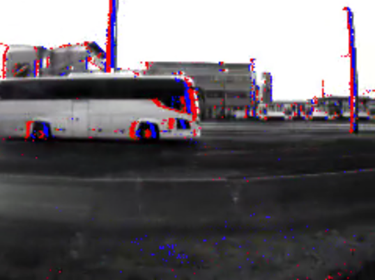
(a)

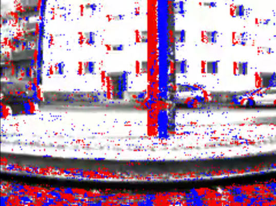
(b)

Figure 2: Example of pole observations on Trajectory 1 (left) and Trajectory 2 (right). For more information about the trajectories, refer to Section IV-A. For visualization purposes, the events are accumulated for one event array(which leads to a motion blur effect in the visualization) and overlaid on a conventional camera image. Illumination increases (positive events) are represented in blue while illumination decreases (negative events) are represented in red.

Figure 2 showcases how typical poles are observed as vertical structures by the DVS for both investigated datasets (see Section IV-A). More examples can be found in our paper video. Due to the unique data stream, novel algorithms need to be devised to achieve real-time performance [17, 18, 19].

Hence, in this work, lines from infrastructure landmarks are detected and tracked in real-time using a concatenation of custom, event-based Hough transforms and further triangulated based on a given odometry. Concisely, the contributions of this work are the following:

• A novel real-time, iterative, event-based HT and Non-Maxima Suppression (NMS) strategy to detect straight edges produced by infrastructure, even at close distances to the vehicle and at high velocities.

• A full real-time mapping pipeline to detect, track and triangulate meaningful landmarks characterized by vertical lines, given an available odometry.

• An evaluation of mapping accuracy and reliability of the whole pipeline on real-world data collected on a tram in Potsdam, Germany. This includes a quantitative evaluation on a shorter track with a high-accuracy surveyed ground truth map and a qualitative evaluation on a longer track segment.

• An in-depth analysis of additional and missed detections.

II Related Work

Railway mapping: To enable train operation which is not limited by the infrastructure-side Balises, current research focuses on on-board localization [5, 20]. Leveraging the unique constraint that rail vehicles can only operate on their tracks, multiple works investigated the use of digital maps of the rail network to improve localization accuracy using GNSS [21, 22, 23], odometry map matching [24] which can be problematic on parallel tracks or long segments, eddy current sensors [25, 26] or IMU vibration patterns [27]. However, the surroundings of the tracks are often not well mapped even though it can be highly informative. Visual mapping using conventional cameras was demonstrated by Wohlfeil et al.  [28], mapping both tracks and switches allowing for global localizations close to the switches. Hough²Map, in contrast, focuses on mapping the more frequent infrastructure elements such as poles, especially visible from a side-facing camera.

Line detection: In order to map such infrastructure elements, vertical lines in the environment need to be detected. Hough [29] introduced an approach for detecting simple shapes like lines in images based on a voting scheme within a pre-defined parameter space. Improvements to the HT over the years include improved line parameterization to better account for vertical lines [30] and performance improvements by introducing adaptive parameter spaces of varying resolutions and searching through them in a hierarchical manner [31, 32] or probabilistic sub-sampling of voting points [33]. By observing the development of peaks in the Hough space (HS) in an incremental probabilistic HT, early stopping can be performed [34]. Dalitz et al.  [35] replaced the NMS with an iterative scheme consisting of a simple maximum search and the subsequent removal of all points from the HS belonging to the current maximum.

A second class of line detectors are based on non-parametric detection [36, 37, 38]. Improved real-time versions, such as Line Segment Detector (LSD) by Grompone von Gioi et al.  [39] and ELSD by Patraucean et al.  [40], allow for fast and accurate detection with minimal false positives.

All aforementioned methods operate on standard gray-scale images. However, to leverage the benefits of event-based vision, most of those algorithms need to be revised and adapted. That is one of the main goals of this paper.

Event-based line detection: Conradt et al. [41] introduced an event-based HT for balancing a pencil, modeling the detected line as a Gaussian in the HS which gets updated by incoming events, allowing for fast updates but limiting the system to just one tracked line. Ni et al.  [42] used a circular HT to track microparticles, reducing the computational load by limiting the parameter space to a fixed specific radius. Glover et al.  [43] introduced a circular HT for detecting and tracking balls in cluttered environments. To reduce the search space the HT is directed, only permitting events which, according to their respective local optical flow, agree with the motion model of the tracked object. The significant problem is the search for the maximum in the HS, which can be solved by the usage of Spiking Neural Networks [44]. Yuan and Ramalingam [45] developed an event-based pose estimation algorithm based on vertical lines in the environment which are detected using a binning scheme similar to a simple HT with a 1D parameter space, thus significantly reducing the possibilities of detectable lines, but enabling real-time performance. Mueggler et al.  [46] introduced a similar event-based pose estimation but for 6 Degrees of Freedom (DoF) using a black square as reference in the event stream. Line detection is performed by updating known lines with events if these are significantly close to the known line. Only the first initialization is performed using a full HT. Bagchi and Chin [47] perform attitude estimation by tracking stars as straight lines in a spatio-temporal space, instead of detecting actual lines in the image space. The estimation is done iteratively per event, but only inside a fixed time window and lacks a decay of old events, it does therefore not continuously track the stars.

As an alternative to a HT, Brandli et al.  [48] introduced an event-based line segment detector similar to the non-parametric methods mentioned above. Le Gentil and Tschopp et al.  [49] detect line segments as locally spatio-temporal planar patches to perform visual-inertial odometry. Both approaches, while promising, are not able to function in real-time in scenarios with high apparent motion, e.g. texture-rich scenes with fast motion. Valeiras et al.  [50] perform event-based line detection by modelling lines in a spatio-temporal space and matching events to line hypothesis using an optical flow for events. In comparison with our approach, they have to limit the maximum number of hypotheses, and have a higher parametrization complexity.

III Hough²Map

In this section, the whole Hough²Map pipeline, as shown in Figure 1, is introduced. First we explain how vertical structures are efficiently detected using an iterative event-based HT and NMS in comparison to a classical full HT. Using a second spatio-temporal HT the structures are tracked over time and subsequently triangulated in combination with an available odometry to obtain their position in the map.

III-A Iterative Hough Transform – Pole Detection

HT [29] is a classic method for detecting lines in images. Given that each line can be represented by a distance $r$ from the top left corner and an angle $\theta$, the Hough space (HS) represents the parameter space of possible lines that are being detected, where each point in the HS corresponds to a line hypothesis. More precisely for a point at image coordinates $\left(u,v\right)$ the added hypotheses in the HS are all points $p_{h}$,

$$p_{h}\in\{(r,\theta)\,|\,r=u\cdot\cos{\theta}+v\cdot\sin{\theta},\theta\in[\,0,\pi]\,\}.$$ (1)

For practical reasons the HS is discretized into $N$ and $M$ intervals for distances and angles, respectively. Thereby, to detect mainly vertical structures, we restricted $\theta\in[\,-10\,\mathrm{{}^{\circ}},10\,\mathrm{{}^{\circ}}]$. After accumulating hypotheses from all points in the image space and adjusting for camera distortions using a pre-computed look-up table, distinct lines in the image space will appear as local maxima in the HS.

To reduce the amount of noise, a NMS procedure is applied to determine the valid maxima in the HS. First, we define the set of local maxima $\mathcal{M}_{l}^{t}$ at timestep $t$ as all points that are above a threshold $T_{\text{Hough}}$ and are larger than all their neighbours in an 8-connected neighbourhood. Additionally, the set of global maxima $\mathcal{M}_{g}^{t}\subseteq\mathcal{M}_{l}^{t}$ includes all local maxima that are bigger than all other local maxima within a defined suppression radius $R$. The objective of NMS is to find $\mathcal{M}_{g}^{t}$ inside the HS, which represents a set of most distinct lines in the image. To perform NMS, all $\mathcal{M}_{l}^{t}$ in the HS are detected and ordered. Afterwards, the ordered $\mathcal{M}_{l}^{t}$ are successively evaluated and marked as belonging to $\mathcal{M}_{g}^{t}$ if there does not already exist another global maximum within the suppression radius.

Detecting lines in a DVS event stream can be achieved by accumulating the events inside a sliding window, applying HT as explained before to this window and retrieving $\mathcal{M}_{g}^{t}$ in the HS. The sliding window is defined as the last $300$ events which were observed by the DVS. When a new event arrives it can be added to the window, the oldest event removed and the line detection can be repeated. A computationally efficient approach is to update the accumulator cells of the HS iteratively per event by only adding the hypotheses of the newest point and similarly removing the ones of the oldest point. This results in two sets of accumulator cells, $\mathcal{P}_{+}$ and $\mathcal{P}_{-}$, which need to be updated for the added and removed event, respectively. The major disadvantage is that at each step a full traversal of the HS is still required to perform NMS, which makes this approach computationally inefficient and prevents real-time operation on a DVS. To tackle this, we developed an iterative NMS for event-streams in Section III-B.

III-B Iterative Non-Maxima Suppression

To perform NMS more efficiently we have to observe that each added or removed event to the iterative HT explained in Section III-A modifies at most ${O(}\max(N,M){)}$ accumulator cells in the HS. Therefore, the changes in the HS per event are minimal. By only examining the two sets of affected accumulator cells $(\mathcal{P}_{+},\mathcal{P}_{-})$ that were increased or decreased by the new or removed event, respectively, we can update the list of global maxima from the previous step $\mathcal{M}_{g}^{t-1}$ to obtain $\mathcal{M}_{g}^{t}$, without having to iterate over the entire HS. A detailed description of the proposed iterative NMS is depicted in Algorithm 1. This implementation of an iterative NMS leads to the exact same results as performing a full NMS for each event, as it considers all possible ways in which $\mathcal{P}_{+}$ and $\mathcal{P}_{-}$ can influence the HS to cause new global maxima to appear or disappear with respect to $\mathcal{M}_{g}^{t-1}$.

1:procedure INMS($\mathcal{P}_{+}^{t},\mathcal{P}_{-}^{t},\mathcal{M}_{g}^{t-1}$)

2: 

3:Phase 1 - Obtain candidates for $\mathcal{M}_{g}^{t}$

4: 

5:   $\mathcal{M}_{g}^{t*}\leftarrow\mathcal{M}_{g}^{t-1}$$\triangleright$ Init list of candidate global maxima

6:   for all $p_{+}\in\mathcal{P}_{+}^{t}$ do

7:     skip $\leftarrow$ false

8:     for all 8-connected neighbours $p^{\prime}_{+}$ of $p_{+}$ do

9:       if HS$(p_{+})$ is equal to HS$(p^{\prime}_{+})$ then

10:         skip $\leftarrow$ true

11:         if $p^{\prime}_{+}\in\mathcal{M}_{g}^{t-1}$ then

12:           Remove $p^{\prime}_{+}$ from $\mathcal{M}_{g}^{t*}$

13:           Add $\left\{m_{l}^{t}\in\mathcal{M}_{l}^{t}\,\big{|}\,||m_{l}^{t}-p^{\prime}_{+}||\leq R\right\}$ to $\mathcal{M}_{g}^{t*}$                      

14:     if not skip then

15:       if $p_{+}\in\mathcal{M}_{l}^{t}$ and $p_{+}\notin\mathcal{M}_{g}^{t-1}$ then

16:         Add $p_{+}$ to $\mathcal{M}_{g}^{t*}$                

17:   for all $p_{-}\in\mathcal{P}_{-}^{t}$  do

18:     for all 8-connected neighbours $p^{\prime}_{-}$ of $p_{-}$ do

19:       if HS$(p_{-})+1$ is equal to HS$(p^{\prime}_{-})$ then

20:         if $p^{\prime}_{-}\in{\mathcal{M}_{l}^{t}}$ then

21:           Add $p^{\prime}_{-}$ to $\mathcal{M}_{g}^{t*}$                      

22:     if $p_{-}\in\mathcal{M}_{g}^{t-1}$ then

23:       Remove $p_{-}$ from $\mathcal{M}_{g}^{t*}$

24:       Add $\left\{m_{l}^{t}\in\mathcal{M}_{l}^{t}\,\big{|}\,||m_{l}^{t}-p_{-}||\leq R\right\}$ to $\mathcal{M}_{g}^{t*}$         

25: 

26:Phase 2 - Detect and apply suppression

27: 

28:   repeat

29:     suppress $\leftarrow$ false

30:     Sort $\mathcal{M}_{g}^{t*}$ in descending order

31:     for all ${}^{i}m^{t}_{g}\in\mathcal{M}_{g}^{t*}$ do

32:       $\mathcal{M}_{s}^{t}\leftarrow\left\{{}^{j}m_{l}^{t}\in\mathcal{M}_{l}^{t}\,\big{|}\,i\neq j,\,||{}^{j}m_{g}^{t}-{}^{i}m_{g}^{t}||\leq R\right\}$

33:       Remove $\mathcal{M}_{s}^{t}$ from $\mathcal{M}_{g}^{t*}$

34:       for all $m_{s}^{t}\in\mathcal{M}_{s}^{t}$ do

35:         for all $m_{g}^{t-1}\in\mathcal{M}_{g}^{t-1}$ do

36:           if $m_{s}^{t}=m_{g}^{t-1}$ then

37:             Add $\left\{m_{l}^{t}\in\mathcal{M}_{l}^{t}\,\big{|}\,||m_{l}^{t}-m_{s}^{t}||\leq R\right\}$ to $\mathcal{M}_{g}^{t*}$

38:             suppress $\leftarrow$ true                                

39:   until suppress is false

40:   $\mathcal{M}_{g}^{t}\leftarrow\mathcal{M}_{g}^{t*}$

41:   return $\mathcal{M}_{g}^{t}$

Algorithm 1 Iterative Non-Maxima Suppression

The algorithm can be divided into roughly two stages. In the first step, based on $\mathcal{P}_{+}$ and $\mathcal{P}_{-}$ as well as $\mathcal{M}_{g}^{t-1}$, we create a list of potential global maxima $\mathcal{M}_{g}^{t*}$, without iterating over the entire HS. This is done by checking four distinct cases, out of which two deal with the direct creation of new potential global maxima. If an accumulator cell in $\mathcal{P}_{+}$ is a local maximum, now it is also a new potential global maximum, and similarly if an accumulator cell in the 8-connected neighbourhood of a cell in $\mathcal{P}_{+}$ just became a new local maxima at time step $t$, it is also a potential new global maxima. The other two cases deal with the potential removal of old global maxima, in which case a more exhaustive search in the suppression radius is required to retrieve the current local maxima that might now have become global maxima. In the second step, we sort the candidate maxima $\mathcal{M}_{g}^{t*}$ and filter out the maxima that are within each others suppression radius. The removal of a maxima candidate that was a global maxima at time step $t-1$ requires the addition of the local maxima surrounding the removed point to the set of candidates $\mathcal{M}_{g}^{t*}$. In this case, the entire second step needs to be repeated, to ensure that none of the new points are within existing suppression radii. After the repeated filtering and suppression step, the remaining candidate maxima are the new global maxima $\mathcal{M}_{g}^{t}$.

Performing a full NMS has a complexity of $O(NM)$, since a full traversal of the HS is required. In contrast the iterative NMS has a varying cost, depending on the number of maxima that change during one step. In the best case scenario, where no changes occur, the complexity is $O(\max(N,M))$, while in the worst case scenario the whole HS will be searched, leading to a complexity of $O(NM)$. In practice though the worst case scenario rarely happens and the iterative NMS is far more efficient than the full NMS (see Section IV-C).

III-C Second Hough Transform – Pole Tracking

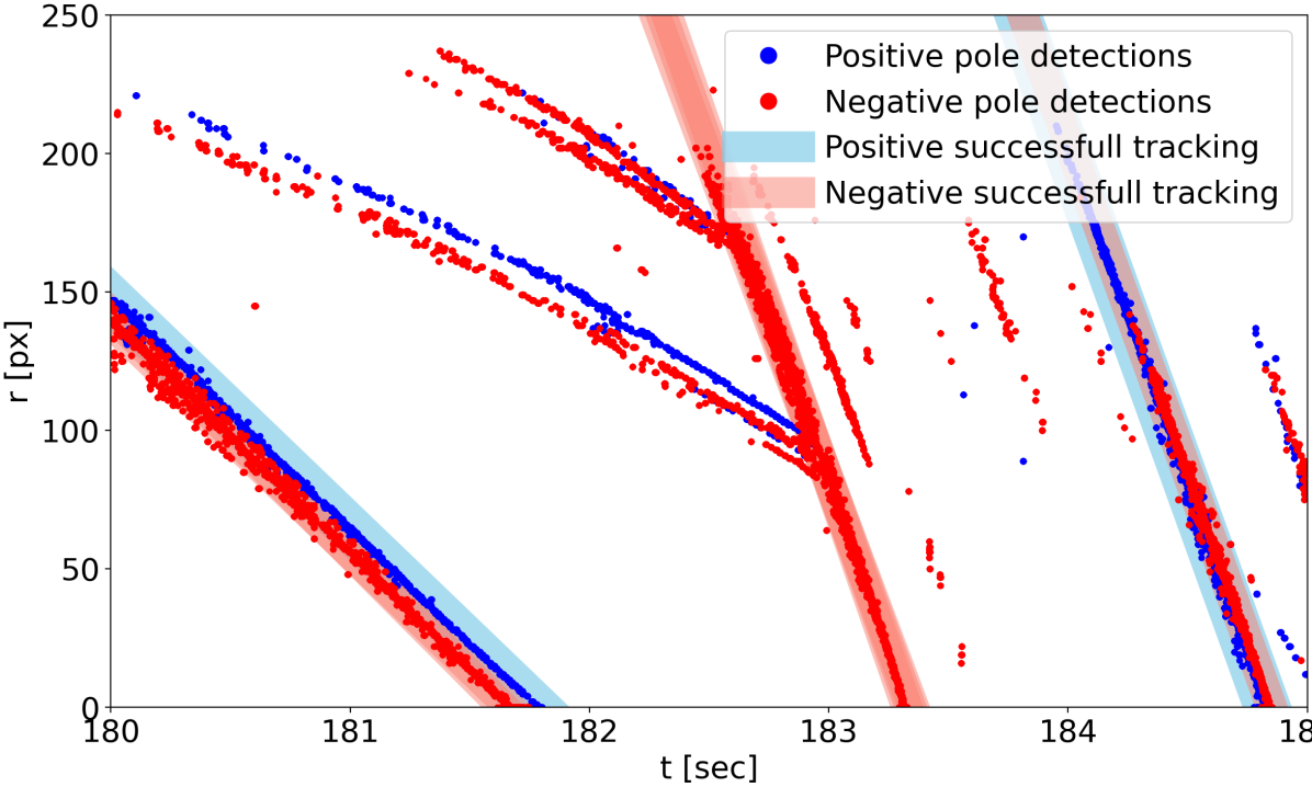
Figure 3: The second HS tracks the horizontal position of line detections over time for both positive and negative events separately. By using the second HT on this spatio-temporal representation, object tracks of corresponding detections can be obtained. The object is only accepted if positive and negative tracks are pairwise, e.g. the middle negative track is discarded.

The next step of the pipeline consists of associating line detections from the same objects across time, in order to triangulate them into map points. We map individual line detections into a spatio-temporal space, by taking the horizontal line positions, as defined by their shortest distance $r$ to the origin (Equation 1), at each time of detection, as shown in Figure 3). Assuming a locally constant train velocity, straight lines in the spatio-temporal space correspond to vertical structures which move at constant speed through the Field of View (FoV) of the camera. This constant velocity assumption only needs to hold true for a very short time, the time a pole is in the cameras FoV, and is justified by the high inertias in typical railway vehicles. A second HT can be applied on the spatio-temporal representation depicted in Figure 3 to associate individual detections with landmarks and obtain landmark tracks $D_{t:t+k}$ containing horizontal line position and timestamp pairs, where $k$ depicts the length of the track. Additionally, we perform the tracking for both the positive and negative events in separate HSs in order to filter detections triggered by positive events which do not have a corresponding detection triggered from negative events or vice versa, such as the second detection in Figure 3. This filters out larger objects such as buildings or bridges, where the positive and negative line detections occur far apart and which are currently out of the scope of this work.

III-D Triangulation

In order to triangulate the tracked detections into landmarks, we leverage position estimates $P_{t:t+k}\in SE(2)$ of the vehicle from an external odometry. Odometries with locally low drift exist based on Doppler radars, wheel encoders [51] or also front facing cameras [6, 7, 52, 53]. Based on a camera calibration, namely the horizontal principal point $u_{0}$ and focal length in pixels $\alpha_{x}$, and samples $D_{t:t+k}$ along the detection track, the landmark position $X$ is obtained using a 2D version of a Direct Linear Transform (DLT) triangulation by assembling a matrix $A\in\mathbb{R}^{k\times 3}$:

$$A[i,j]=(D_{t+i}-u_{0})/\alpha_{x}\cdot P_{t+i}[1,j]-P_{t+i}[0,j],\\$$ (2)

where $i,j$ are matrix indices. After computing the Singular Value Decomposition (SVD) of A, i.e. $U\cdot\Sigma\cdot V^{*}=\operatorname{SVD}(A)$, we take the least significant right-singular vector of $V^{*}$, which corresponds to the homogeneous representation of $X$ and just needs to be normalized [54].

IV Experimental Evaluation

To evaluate the accuracy and performance of Hough²Map, we performed multiple experiments on real-world railway datasets. Furthermore, an evaluation is performed to compare the iterative HT and NMS to their conventional counterparts. Although a comparison with  [50] would be informative, at the time of this publication the authors had not made neither the data nor implementation publicly available.

IV-A Datasets

The pipeline was evaluated on two available datasets from a tram in Potsdam, Germany [6]. Trajectory 1 is recorded on the Betriebshof, a short $815\,\mathrm{m}$ circular track with a large variety of visual features and challenging situations including significant velocity changes. For this track a high accuracy manually surveyed map of nearly all poles exists which will be used as ground truth for the evaluation of the accuracy of the pipeline. Trajectory 2 is a longer $2545\,\mathrm{m}$ section of a public tram line passing through rural, (sub-)urban areas and forests with a more constant vehicle velocity and is therefore a more realistic scenario for everyday railway operation. Unfortunately, for Trajectory 2 no accurate ground truth map was available. To perform a qualitative evaluation pole positions were manually annotated from high-resolution satellite imagery and aligned to GNSS coordinates.

IV-B Hardware Setup

IV-B1 Devices

The dataset was recorded using an iniVation Dynamic and Active Vision Sensor (DAVIS) 240 [55] with a sensor size of $240\times 180\,\mathrm{px}$, a minimum latency of $12\,\mathrm{\mu s}$ and a horizontal FoV of $56\,\mathrm{{}^{\circ}}$. The device was oriented perpendicular to the axis of motion of the tram out of a side window as shown in Figure 4. This enables a good observability of the environment close to the track and results in a linear perceived motion of detections through the FoV enabling easy tracking. As the goal of this evaluation is to assess the accuracy of the detection and mapping pipeline, a high-accuracy Inertial Navigation System (INS) is used as odometry as opposed to drifting odometries to avoid external error sources.

IV-B2 Calibration

The intrinsic camera calibration parameters of the DAVIS were obtained using the Kalibr toolbox [56] on the active pixels. At the time of the recording of the dataset no appropriate calibration procedure for the extrinsic calibration of the camera relative to the train was available. This was therefore obtained through manual tuning of the lateral and longitudinal offset along the train.

IV-C Iterative Hough Transform and Non-Maxima Supression

To mainly detect vertical lines in the full image, the HS was chosen as $r\in\left[0\,\mathrm{px},260\,\mathrm{px}\right]$ and $\theta\in\left[-10\,\mathrm{{}^{\circ}},10\,\mathrm{{}^{\circ}}\right]$ in $1\,\mathrm{{}^{\circ}}$ increments. In order to compare the performance of our iterative HT and NMS against the conventional version with a Full-NMS, we compared the resulting output of the detection stage (without tracking and mapping) on the Trajectory 1 dataset. A comparison of each individual detection showed that both variants provide the exact same output. On average the processing of an event in the full HT took $6.04\,\mathrm{\mu s}$ per event $e$ with a maximum of $30.27\,\nicefrac{\mathrm{\mu s}}{\mathrm{e}}$. In comparison, our iterative variant took on average $0.65\,\nicefrac{\mathrm{\mu s}}{\mathrm{e}}$ with a maximum of $6.20\,\nicefrac{\mathrm{\mu s}}{\mathrm{e}}$. For event rate statistics, see Section IV-E.

IV-D Detection Reliability and Accuracy

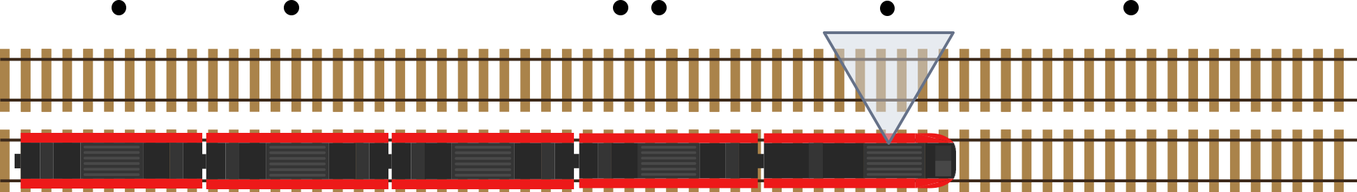
Figure 4: The DVS in a perpendicular setup to the direction of motion of the train, observing the environment passing by.

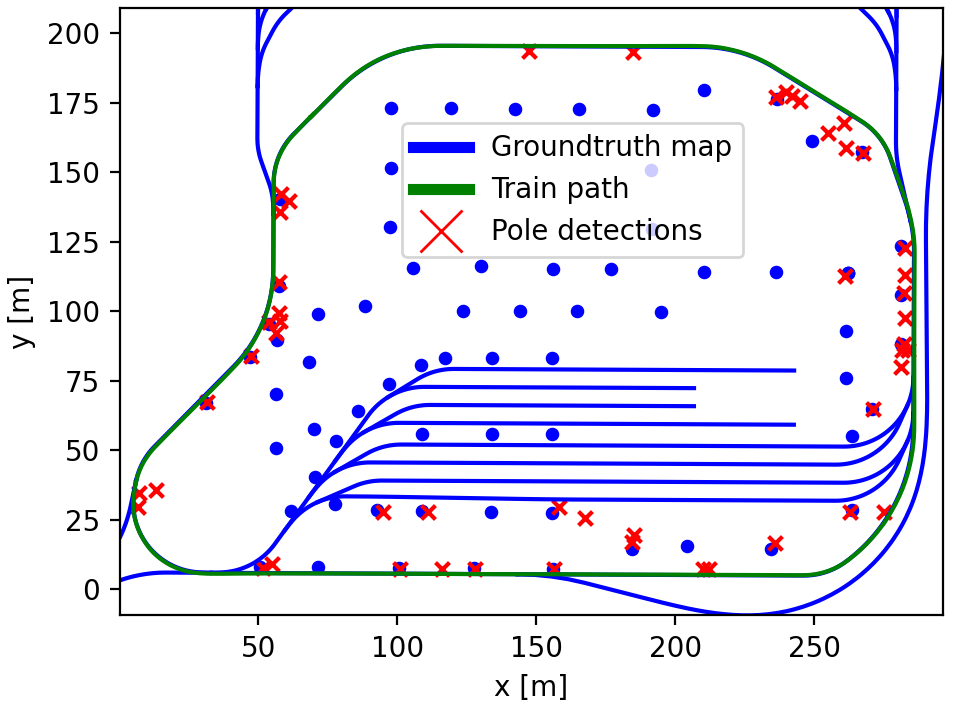
Figure 5: Infrastructure map of Trajectory 1. Many of the ground truth poles in the center of the loop are occluded from the camera and therefore cannot be mapped. Some false positives are discussed in detail in Section IV-D.

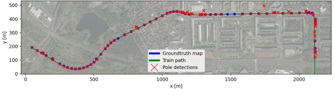
Figure 6: Infrastructure map of Trajectory 2 overlaid on a satellite image including pole detections and manual annotations.

Due to the differences between the datasets as well as the available ground truth data, evaluations are performed differently for each dataset. For Trajectory 1 an accurate ground truth of pole positions is available. Therefore, both the reliability of detecting poles or wrongly detecting other objects, as well as the accuracy of the triangulation can be evaluated. The accuracy is reported as a Root Mean Square Error (RMSE) over all matching detections. As the manual annotation for Trajectory 2 is a fairly inaccurate process, evaluations will be carried out only for the detection reliability and not for the mapping accuracy.

The full pipeline as described in Section III was tested on both datasets. All parameters, such as HS thresholds, integration window sizes and NMS suppression radii were kept constant over both experiments. Figures 5 and 6 show the resulting maps for the respective datasets including pole detections, GNSS odometry and ground truth data.

IV-D1 Detection reliability

TABLE I: Pole detection reliability of the pipeline.

	Trajectory 1	Trajectory 2
Ground truth	43	65
True Positives	23	60
False Negatives	20	5
False Positives	27	28

The reliability evaluation results of the mapping pipeline on both datasets can be found in Table I. On Trajectory 1, out of 43 known poles in a range of $25\,\mathrm{m}$ to the tram track 23 were detected successfully. In addition 27 other objects were included in the detections as seen in Table II. These mostly consisted of objects which are visually similar to poles or infrastructure adjacent to buildings, such as chimneys or rain pipes, but which were not detailed in the available ground truth data. Furthermore, many poles in the ground truth map are quite far away from the tram track, making a reliable detection difficult due to occlusions, FoV of the camera, and limited camera resolution. Further complications are caused by a strongly varying velocity profile of the tram during this test drive, which is rather uncharacteristic during normal operation. This leads to occasional violations of the constant velocity assumption specified in Section III-C. These properties make Trajectory 1 a rather challenging dataset.

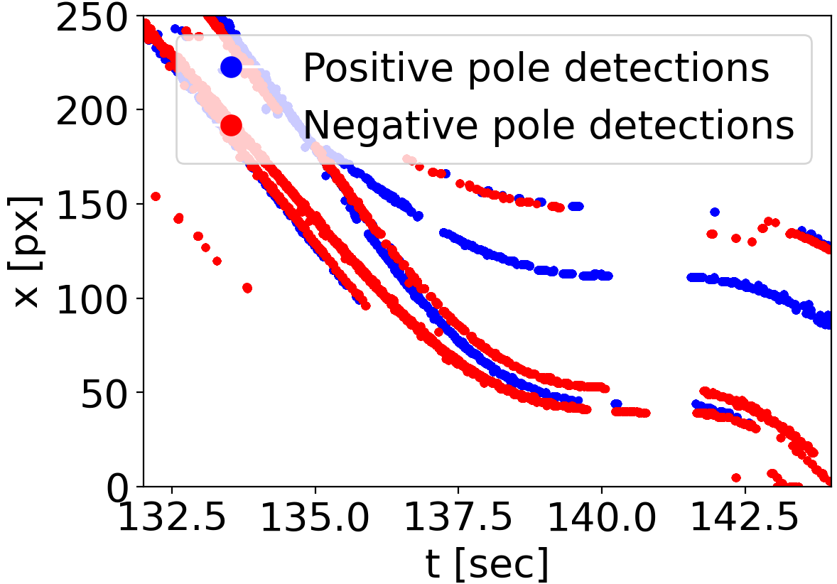
(a) Changing velocity

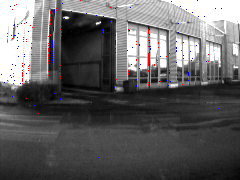
(b) Slow speed

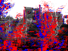
(c) Poles occluded by vegetation

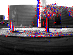
(d) Chimney

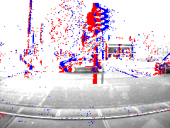
(e) Street signs

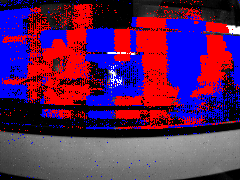
(f) Other tram

Figure 7: (a) shows the spatio-temporal domain in which poles are tracked by the second HT (b)-(f) show the DVS visualization as in Figure 2 to highlight the characteristics of generated events in certain situations and how these might lead to failure cases. (a) and (b) Missed detections due to slow and changing velocity. (c) Missed detection due to partial occlusion and noise. (d) Detections of unmapped objects such as a chimney. (e) Street signs and signals wrongly detected as poles. (f) Another tram passing by with its window edges causing false detections.

TABLE II: Distribution and origin of false positive detections

	Trajectory 1	Trajectory 2
Unmapped poles	8	7
Adjacent to buildings	17	2
Trees	1	2
Street Signs	1	11
Other Train	0	6
Total	27	28

On Trajectory 2 out of 65 known poles 60 were detected successfully. There were however also 28 false positive detections from various sources. As most known poles are closer to the track and as the tram keeps a more steady velocity, this trajectory better agrees with our assumptions of constant velocity and represents a more realistic scenario. However, due to the manual annotation process, ground truth data might be incomplete, as several poles were not recognizable due to vegetation or challenging lighting in the satellite image. An in-depth analysis of missed and wrong detections revealed several distinct reasons reported in Figure 7 and Table II:

• Most commonly, manually set thresholds in the HSs incorrectly filter out poles, such as when these are too small, too far away or occluded by surrounding vegetation (Figure 7c).

• Multiple poles located close to each other can get filtered by the suppression radius of the NMS.

• Drastic changes in vehicle speed during a pole observation significantly violate the constant velocity assumption of the second HT resulting in a non-straight line for the pole in the $x-t$ space visible in Figure 7a.

• Very slow speeds result in minimal changes in illumination and a very low event rate mainly dominated by sensor noise as shown in Figure 7b.

Potential measures to improve are adaptive thresholds and sensor settings based on the observed environments, or vehicle speed compensation in the $x-t$ space. Furthermore, if scenarios with highly varying speeds become relevant, a set of Extended Kalman Filters could be used to track pole detections.

Main reasons for additional pole detections include:

• From the DAVIS video stream a total of 15 poles can additionally be confirmed as correctly detected, but a corresponding ground truth pole is missing as the ground truth data for both trajectories is incomplete.

• Street signs or signals (Figure 7e) located near the track resemble poles closely resulting in a detection.

• At one point in time another tram passes through the FoV of the camera (Figure 7f), causing several wrong detections over a short amount of time. Such false positives could be filtered by a minimal distance threshold from the camera, as the additional speed of the other vehicle would result in a very small triangulated depth.

• On rare occasions trees and special features adjacent to buildings, such as chimneys, are also detected (Figure 7d).

Many of the false positives correspond to infrastructure objects that can be consistently mapped. Therefore, for the purpose of railway localization, such objects are not a drawback of our approach but an opportunity to get even more good landmarks into the map.

IV-D2 Accuracy evaluation

In a second step we evaluated the accuracy of our mapping pipeline. Detections were matched to ground truth pole positions through a simple nearest-neighbor scheme with a rejection radius of $4\,\mathrm{m}$. From the matching set of detections the RMSE can be computed with a value of $1.1518\,\mathrm{m}$. This magnitude of error is acceptable for the target application since landmarks can still be distinctively associated for the purpose of localization. Furthermore, the error consists of a longitudinal shift along the axis of motion with an average of $1.0045\,\mathrm{m}$ and a lateral shift with an average of $0.73748\,\mathrm{m}$. In an ETCS context [57], a good localization perpendicular to the axis of motion is of higher importance to facilitate track selectivity. Even though both reported errors are within the same order of magnitude, the lower error in lateral direction suggests a high potential to enable track selective localization. Please note however, that the mapping accuracy does not directly correspond to a possible pose estimation accuracy but reflects the global error of placing infrastructure elements into the map.

IV-E Processing Time

Table III provides an overview of event rate $\epsilon$ statistics, namely the number of events per second, processing times $t_{p}$ of a parallelized version of the whole pipeline and real time factors on both datasets, corresponding to the total CPU load. The size of the parameter space was chosen to be $21\times 260$. All data was processed on an Intel i7-9750H CPU with $16\,\mathrm{GB}$ of memory. Thanks to the iterative implementation of HT and NMS, our pipeline easily achieves real-time performance resulting in an average total CPU load of $41\,\mathrm{\%}$ and $59\,\mathrm{\%}$ for Trajectory 1 and Trajectory 2, respectively, while still allowing the system to perform other tasks like visual odometry, localization on the same platform or enable real-time processing also for higher vehicle velocities. For a stable control architecture, a constant frequency of the pipeline is desirable. Running the pipeline also for the cases with very high event rates, for a maximum of $11.5\,\mathrm{\%}$ of event arrays, the processing of the subsequent event array had to be buffered. In a delay sensitive application, this can be tackled by randomly sub-sampling events in case of a very high event rate.

TABLE III: Event rate $\epsilon$ statistics of the received sensor data, processing time $t_{p}$, as well as a real-time factor describing the required processing time compared to the rate of new sensor measurements (total CPU load). $\bar{\cdot}$: Average, max: maximum, StD: standard deviation

	Trajectory 1	Trajectory 2
$\bar{\epsilon}$	$115633\,\nicefrac{\mathrm{e}}{\mathrm{s}}$	$204909\,\nicefrac{\mathrm{e}}{\mathrm{s}}$
$\epsilon_{max}$	$824705\,\nicefrac{\mathrm{e}}{\mathrm{s}}$	$1197064\,\nicefrac{\mathrm{e}}{\mathrm{s}}$
$\epsilon_{StD}$	$133443\,\nicefrac{\mathrm{e}}{\mathrm{s}}$	$146519\,\nicefrac{\mathrm{e}}{\mathrm{s}}$
$\bar{t_{p}}$	$3.55\,\nicefrac{\mathrm{\mu s}}{\mathrm{e}}$	$2.89\,\nicefrac{\mathrm{\mu s}}{\mathrm{e}}$
$t_{p,max}$	$127.8\,\nicefrac{\mathrm{\mu s}}{\mathrm{e}}$	$117.7\,\nicefrac{\mathrm{\mu s}}{\mathrm{e}}$
$t_{p,StD}$	$5.13\,\nicefrac{\mathrm{\mu s}}{\mathrm{e}}$	$3.47\,\nicefrac{\mathrm{\mu s}}{\mathrm{e}}$
Real time factor	0.41	0.59
Delayed event arrays	$1.3\,\mathrm{\%}$	$11.5\,\mathrm{\%}$

V Conclusion

In this paper we introduced Hough²Map, a high-speed real-time infrastructure mapping pipeline for utilization in a railway localization pipeline. We developed a novel iterative HT and NMS for asynchronous event-based data as a method to detect typical railway infrastructure represented by vertical lines even at close range and high speeds. Hough²Map subsequently tracks detections over time in order to triangulate and map each object.

We validate our pipeline on two different datasets including real-life scenarios as well as a more challenging trajectory including occlusions, varying speeds and excess noise from close-by vegetation. Our experiments show that Hough²Map is capable of reliably and accurately detecting and mapping poles and other infrastructure elements at close range even at high speeds, but, as expected, have difficulties with objects that are positioned further away.

We plan to expand this work into a full railway localization pipeline exploiting previously recorded maps of the poles to perform accurate high-speed localization.

GNSS

Global Navigation Satellite System

IMU

Inertial Measurement Unit

DVS

Dynamic Vision Sensor

SLAM

Simultaneous Localization and Mapping

DAVIS

Dynamic and Active Vision Sensor

SNN

Spiking Neural Network

DoF

Degrees of Freedom

NMS

Non-Maxima Suppression

ETCS

European Train Control System

MAV

Micro Aerial Vehicle

LSD

Line Segment Detector

HT

Hough transform

HS

Hough space

FoV

Field of View

RTK

Real-Time Kinematic

RMSE

Root Mean Square Error

INS

Inertial Navigation System

EKF

Extended Kalman Filter

DLT

Direct Linear Transform

SVD

Singular Value Decomposition

References

- [1] O. Stalder, ETCS for Engineers. DVV Media Group GmbH, 2011.
- [2] J. Beugin and J. Marais, “Simulation-based evaluation of dependability and safety properties of satellite technologies for railway localization,” Transportation Research Part C: Emerging Technologies, 2012.
- [3] J. Marais, J. Beugin, and M. Berbineau, “A Survey of GNSS-Based Research and Developments for the European Railway Signaling,” IEEE Transactions on Intelligent Transportation Systems, no. 10, 2017.
- [4] T. Albrecht, K. Lüddecke, and J. Zimmermann, “A precise and reliable train positioning system and its use for automation of train operation,” in IEEE Int. Conf. on Intelligent Rail Transportation, 2013.
- [5] J. Otegui, A. Bahillo, I. Lopetegi, and L. E. Díez, “A Survey of Train Positioning Solutions,” IEEE Sensors Journal, no. 15, 2017.
- [6] F. Tschopp, T. Schneider, A. W. Palmer, N. Nourani-Vatani, C. Cadena, R. Siegwart, and J. Nieto, “Experimental comparison of visual-aided odometry methods for rail vehicles,” IEEE Robotics and Automation Letters, no. 2, 2019.
- [7] D. Burschka, C. Robl, and S. Ohrendorf-Weiss, “Optical Navigation in Unstructured Dynamic Railroad Environments,” arXiv preprint arXiv:2007.03409, 2020.
- [8] M. Burri, H. Oleynikova, M. W. Achtelik, and R. Siegwart, “Real-time visual-inertial mapping, re-localization and planning onboard MAVs in unknown environments,” in IEEE Int. Conf. on Intelligent Robots and Systems, 12 2015.
- [9] M. Fehr, T. Schneider, and R. Siegwart, “Visual-Inertial Teach and Repeat Powered by Google Tango,” in 2018 IEEE/RSJ International Conference on Intelligent Robots and Systems (IROS), 10 2018.
- [10] M. Bürki, C. Cadena, I. Gilitschenski, R. Siegwart, and J. Nieto, “Appearance‐based landmark selection for visual localization,” Journal of Field Robotics, no. 6, 9 2019.
- [11] C. Arth, M. Klopschitz, G. Reitmayr, and D. Schmalstieg, “Real-time self-localization from panoramic images on mobile devices,” 10th IEEE International Symposium on Mixed and Augmented Reality, ISMAR, 2011.
- [12] S. Lynen, M. Bosse, P. Furgale, and R. Siegwart, “Placeless place-recognition,” International Conference on 3D Vision, 2014.
- [13] S. Lynen, T. Sattler, M. Bosse, J. Hesch, M. Pollefeys, and R. Siegwart, “Get Out of My Lab: Large-scale, Real-Time Visual-Inertial Localization,” Robotics: Science and Systems, no. November, 2015.
- [14] M. A. Mahowald, “VLSI analogs of neuronal visual processing: a synthesis of form and function,” Dissertation (Ph.D.), California Institute of Technology, May 1992.
- [15] P. Lichtsteiner, C. Posch, T. Delbruck, and S. Member, “A 128x128 120 dB 15 s Latency Asynchronous Temporal Contrast Vision Sensor,” IEEE Journal of Solid-State Circuits, no. 2, 2008.
- [16] C. Brandli, R. Berner, Minhao Yang, Shih-Chii Liu, and T. Delbruck, “A 240 x 180 130 dB 3 us Latency Global Shutter Spatiotemporal Vision Sensor,” IEEE Journal of Solid-State Circuits, no. 10, 10 2014.
- [17] R. Benosman, S. H. Ieng, C. Clercq, C. Bartolozzi, and M. Srinivasan, “Asynchronous frameless event-based optical flow,” Neural Networks, 2012.
- [18] R. Benosman, C. Clercq, X. Lagorce, S. H. Ieng, and C. Bartolozzi, “Event-based visual flow,” IEEE Trans. Neural Netw. Learn. Syst., 2014.
- [19] E. Mueggler, H. Rebecq, G. Gallego, T. Delbruck, and D. Scaramuzza, “The event-camera dataset and simulator: Event-based data for pose estimation, visual odometry, and SLAM,” Int. Journal of Robotics Research, no. 2, 2017.
- [20] B. Siebler, O. Heirich, S. Sand, and U. D. Hanebeck, “Joint Train Localization and Track Identification based on Earth Magnetic Field Distortions,” in 2020 IEEE/ION Position, Location and Navigation Symposium (PLANS), 2020.
- [21] K. Gerlach and M. M. Zu Hörste, “A precise digital map for GALILEO-based train positioning systems,” 2009 9th International Conference on Intelligent Transport Systems Telecommunications, ITST 2009, 2009.
- [22] C. Hasberg, S. Hensel, and C. Stiller, “Simultaneous localization and mapping for path-constrained motion,” IEEE Transactions on Intelligent Transportation Systems, no. 2, 6 2012.
- [23] O. Heirich, P. Robertson, and T. Strang, “RailSLAM - Localization of rail vehicles and mapping of geometric railway tracks,” in IEEE Int. Conf. on Robotics and Automation, 2013.
- [24] H. Winter, V. Willert, and J. Adamy, “Train-borne Localization Exploiting Track-Geometry Constraints-A Practical Evaluation,” Tech. Rep., 2020.
- [25] F. Böhringer and A. Geistler, “Location in railway traffic: Generation of a digital map for secure applications,” WIT Transactions on the Built Environment, 2006.
- [26] S. Hensel, C. Hasberg, and C. Stiller, “Probabilistic rail vehicle localization with eddy current sensors in topological maps,” IEEE Transactions on Intelligent Transportation Systems, no. 4, 2011.
- [27] O. Heirich, A. Steingass, A. Lehner, and T. Strang, “Velocity and location information from onboard vibration measurements of rail vehicles,” IEEE Information Fusion, 2013.
- [28] J. Wohlfeil, “Vision based rail track and switch recognition for self-localization of trains in a rail network,” in IEEE Intelligent Vehicles Symposium, 2011.
- [29] P. V. C. Hough, “A method and means for recognition complex patterns; US Patent: US3069654A,” 1962.
- [30] R. O. Duda and P. E. Hart, “Use of the Hough Transformation to Detect Lines and Curves in Pictures,” Communications of the ACM, no. 1, 1972.
- [31] J. Kittler and J. Illingworth, “The Adaptive Hough Transform,” IEEE Transactions on Pattern Analysis and Machine Intelligence, no. 5, 1987.
- [32] H. Li, M. A. Lavin, and R. J. Le Master, “Fast Hough transform: A hierarchical approach,” Computer Vision, Graphics and Image Processing, 1986.
- [33] J. Matas, C. Galambos, and J. Kittler, “Robust detection of lines using the progressive probabilistic hough transform,” Computer Vision and Image Understanding, no. 1, 2000.
- [34] A. YlaJaaski and N. Kiryati, “Adaptive Termination of Voting in the Probabilistic Circular Hough Transform,” IEEE Transactions on Pattern Analysis and Machine Intelligence, no. 9, 1994.
- [35] C. Dalitz, T. Schramke, and M. Jeltsch, “Iterative hough transform for line detection in 3D point clouds,” Image Processing On Line, 2017.
- [36] A. Etemadi, “Robust segmentation of edge data,” in 1992 International Conference on Image Processing and its Applications, 1992.
- [37] J. B. Burns, A. R. Hanson, and E. M. Riseman, “Extracting Straight Lines,” IEEE Trans. Pattern Anal. Mach. Intell., 1986.
- [38] P. Kahn, L. Kitchen, and E. Riseman, “A Fast Line Finder for Vision-Guided Robot Navigation,” IEEE Trans. Pattern Anal. Mach. Intell., 1990.
- [39] R. Grompone Von Gioi, J. Jakubowicz, J. M. Morel, and G. Randall, “LSD: A fast line segment detector with a false detection control,” IEEE Trans. Pattern Anal. Mach. Intell., 2010.
- [40] V. Pǎtrǎucean, P. Gurdjos, and R. G. Von Gioi, “A parameterless line segment and elliptical arc detector with enhanced ellipse fitting,” in European Conference on Computer Vision, 2012.
- [41] J. Conradt, M. Cook, R. Berner, P. Lichtsteiner, R. J. Douglas, and T. Delbruck, “A pencil balancing robot using a pair of AER dynamic vision sensors,” IEEE Int. Symposium on Circuits and Systems, 2009.
- [42] Z. Ni, C. Pacoret, R. Benosman, S. Ieng, and S. Régnier, “Asynchronous event-based high speed vision for microparticle tracking,” Journal of Microscopy, no. 3, 2012.
- [43] A. Glover and C. Bartolozzi, “Event-driven ball detection and gaze fixation in clutter,” IEEE Int. Conf. on Intelligent Robots and Systems, 2016.
- [44] S. Seifozzakerini, W. Y. Yau, B. Zhao, and K. Mao, “Event-based hough transform in a spiking neural network for multiple line detection and tracking using a dynamic vision sensor,” British Machine Vision Conference 2016, BMVC 2016, 2016.
- [45] W. Yuan and S. Ramalingam, “Fast localization and tracking using event sensors,” IEEE Int. Conference on Robotics and Automation, 2016.
- [46] E. Mueggler, B. Huber, and D. Scaramuzza, “Event-based, 6-DOF pose tracking for high-speed maneuvers,” IEEE International Conference on Intelligent Robots and Systems, 2014.
- [47] S. Bagchi and T.-J. Chin, “Event-based Star Tracking via Multiresolution Progressive Hough Transforms,” in 2020 IEEE Winter Conference on Applications of Computer Vision (WACV). IEEE, mar 2020.
- [48] C. Brandli, J. Strubel, S. Keller, D. Scaramuzza, and T. Delbruck, “ELiSeD-An event-based line segment detector,” 2016 2nd International Conference on Event-Based Control, Communication, and Signal Processing, EBCCSP 2016 - Proceedings, no. December 2017, 2016.
- [49] C. L. Gentil, F. Tschopp, I. Alzugaray, T. Vidal-Calleja, R. Siegwart, and J. Nieto, “IDOL: A Framework for IMU-DVS Odometry using Lines,” arXiv preprint arXiv:2008.05749, 8 2020.
- [50] D. Reverter Valeiras, X. Clady, S. H. Ieng, and R. Benosman, “Event-Based Line Fitting and Segment Detection Using a Neuromorphic Visual Sensor,” IEEE Trans. Neural Netw. Learn. Syst, 2019.
- [51] A. W. Palmer and N. Nourani-Vatani, “Robust Odometry using Sensor Consensus Analysis,” in IEEE International Conference on Intelligent Robots and Systems (accepted), 2018.
- [52] F. Tschopp, M. Riner, M. Fehr, L. Bernreiter, F. Furrer, T. Novkovic, A. Pfrunder, C. Cadena, R. Siegwart, and J. Nieto, “VersaVIS—An Open Versatile Multi-Camera Visual-Inertial Sensor Suite,” Sensors, 2020.
- [53] B. Bah, E. Jungabel, M. Kowalska, C. Leithäuser, A. Pandey, and C. Vogel, “ECMI-report Odometry for train location,” 2009.
- [54] R. Hartley and A. Zisserman, “Structure Computation,” in Multiple View Geometry in Computer Vision, 2nd ed., 2004, ch. 12.
- [55] iniVation AG, “DAVIS 240 Datasheet,” 2019. [Online]. Available: https://inivation.com/wp-content/uploads/2019/08/DAVIS240.pdf
- [56] P. Furgale, J. Rehder, and R. Siegwart, “Unified temporal and spatial calibration for multi-sensor systems,” in IEEE Int. Conf. on Intelligent Robots and Systems, 2013.
- [57] Localization Working Group (LWG), “Railways Localisation System High Level Users’ Requirements,” EEIG ERTMS Users Group, Tech. Rep., 12 2019.