Diffusion coefficient matrix of the strongly interacting quark-gluon plasma

Abstract

We study the diffusion properties of the strongly interacting quark-gluon plasma (sQGP) and evaluate the diffusion coefficient matrix for the baryon $(\mathrm{B})$, strange $(\mathrm{S})$ and electric $(\mathrm{Q})$ charges - $\kappa_{qq^{\prime}}$ ($q,q^{\prime}=\mathrm{B},\mathrm{S},\mathrm{Q}$) and show their dependence on temperature $T$ and baryon chemical potential $\mu_{\mathrm{B}}$. The non-perturbative nature of the sQGP is evaluated within the Dynamical Quasi-Particle Model (DQPM) which is matched to reproduce the equation of state of the partonic matter above the deconfinement temperature $T_{c}$ from lattice QCD. The calculation of diffusion coefficients is based on two methods: i) the Chapman-Enskog method for the linearized Boltzmann equation, which allows to explore non-equilibrium corrections for the phase-space distribution function in leading order of the Knudsen numbers as well as ii) the relaxation time approximation (RTA). In this work we explore the differences between the two methods. We find a good agreement with the available lattice QCD data in case of the electric charge diffusion coefficient (or electric conductivity) at vanishing baryon chemical potential as well as a qualitative agreement with the recent predictions from the holographic approach for all diagonal components of the diffusion coefficient matrix. The knowledge of the diffusion coefficient matrix is also of special interest for more accurate hydrodynamic simulations.

I Introduction

An exploration of the properties of hot and dense matter - created in heavy-ion collisions (HICs) at relativistic energies - is in the focus of extensive research. It is the primary goal of experimental programs of the LHC (Large-Hadron-Collider) at CERN, the RHIC (Relativistic Heavy Ion Collider) at BNL, the future FAIR (Facility for Antiproton and Ion Research) at GSI, and the NICA (Nuclotron-based Ion Collider fAcility) facility at JINR, which reproduce in the laboratory the extreme conditions of the early stages of our universe by ’tiny bangs’. In the central region of heavy-ion collisions the deconfined QCD (Quantum Chromo Dynamics) matter – a quark-gluon plasma (QGP) - is created which can achieve an approximate local equilibrium and exhibit hydrodynamic flow Ollitrault (1992); Heinz and Kolb (2002); Shuryak (2009). The hydrodynamic behaviour of the fluid can be characterized by transport coefficients such as shear $\eta$, bulk $\zeta$ viscosities, and diffusion coefficients $\kappa$, which describe the fluid’s dissipative corrections at leading order. The interpretation of the experimental data, and especially the elliptic flow $v_{2}$, in terms of the hydrodynamic models showed that the QGP behaves almost as a nearly perfect fluid with a very low shear viscosity to entropy density ($s$) ratio, $\eta/s$, which reflects that its properties correspond to nonperturbative, strongly interacting matter Shuryak (2005); Gyulassy and McLerran (2005); Romatschke and Romatschke (2007).

By performing an experimental energy scan of HICs one can explore the different stages of the QCD phase diagram. At ultra-relativistic heavy-ion collisions at LHC and RHIC energies, the QGP is created at very large temperatures $T$ and almost zero or low baryon chemical potential $\mu_{\mathrm{B}}$, where according to lattice QCD (lQCD) results Cheng et al. (2008); Aoki et al. (2009) the transition from the QGP to the hadronic matter is a crossover. By reducing the collision energy one can also explore the large $\mu_{\mathrm{B}}$ region where one might expect the existence of a critical point and a 1st order phase transition. Such conditions are presently under investigation within the RHIC BES (Beam Energy Scan) experiments and in future by the FAIR and NICA facilities.

The theoretical description of the QCD matter at finite $\mu_{\mathrm{B}}$, and especially in the vicinity of the critical point, requires an appropriate description of transport of conserved charges – baryon $B$, strangeness $S$ and electric $Q$ charges. In order to study the phenomenon of baryon-stopping, the baryon diffusion was recently introduced to various fluid dynamic models Denicol et al. (2018); Li and Shen (2018); Du and Heinz (2019). Moreover, the baryon diffusion coefficient has been studied in Refs. Arnold et al. (2003); Rougemont et al. (2015); Greif et al. (2018); Ghiglieri et al. (2018); Fotakis et al. (2020); Soloveva et al. (2020a).

In the recent past we have addressed the coupling of the conserved baryon number, strangeness and electric charge; the diffusion coefficient matrix ($\kappa_{qq^{\prime}}$, where $q,q^{\prime}=\mathrm{B},\mathrm{S},\mathrm{Q}$) was introduced and evaluated for a hadron gas and a simple model for quark-gluon plasma (QGP) Greif et al. (2018); Fotakis et al. (2020). These investigations were followed by a more extended study in the hadronic phase from kinetic theory in the case of the electric cross-conductivities Rose et al. (2020). Furthermore, a first study on the impact of the coupling of baryon number and strangeness was provided in Ref. Fotakis et al. (2020). For this the diffusion coefficient matrix of hot and dense nuclear matter has to be investigated thoroughly being important for accurate hydrodynamic simulations. It was further motivated that the off-diagonal coefficients may have implications on the chemical-composition of the hadronic phase Rose et al. (2020).

The study of the transport of conserved electric charge $Q$ during heavy-ion collisions has been in the focus of intensive research. Due to its importance for the description of soft photon spectra and rates Turbide et al. (2004); Akamatsu et al. (2011); Linnyk et al. (2016a); Yin (2014) as well as for hydrodynamic approaches modelling the generation and evolution of electromagnetic fields Tuchin (2013); Inghirami et al. (2019); Denicol et al. (2019); Oliva (2020), much attention was paid to the electric conductivity within different theoretical approaches for the evaluation of the properties of the partonic and hadronic matter Arnold et al. (2000); Brandt et al. (2013); Torres-Rincon (2012); Finazzo and Noronha (2014); Amato et al. (2013); Marty et al. (2013); Aarts et al. (2015); Greif et al. (2014); Puglisi et al. (2014, 2015); Brandt et al. (2016); Rougemont et al. (2015); Ding et al. (2016); Greif et al. (2016); Thakur et al. (2017); Rougemont et al. (2017); Greif et al. (2018); Hammelmann et al. (2019); Soloveva et al. (2020a); Fotakis et al. (2020); Rose et al. (2020).

The exploration of the QGP properties at finite ($T,\mu_{\mathrm{B}}$) are of special interest for an understanding of the phase transition. The transport properties of the strongly interacting QGP has been studied using the Dynamical Quasi-Particle Model(DQPM) Peshier and Cassing (2005); Cassing (2007a, b); Linnyk et al. (2016b); Berrehrah et al. (2016a) that is matched to reproduce the equation of state of the partonic system above the deconfinement temperature $T_{c}$ from lattice QCD. The DQPM is based on a propagator representation with complex self energies which describes the degrees of freedom of the QGP in terms of strongly interacting dynamical quasiparticles which reflect the non-perturbative nature of the QCD in the vicinity of the phase transition where the QCD coupling grows rapidly with decreasing temperature according to lQCD calculations Kaczmarek et al. (2004). Moreover, the DQPM allows to explore the properties of the QGP at finite $(T,\mu_{\mathrm{B}})$, expressed in terms of transport coefficients such as shear $\eta$, bulk $\zeta$ viscosities, baryon diffusion coefficients $\kappa_{B}$ and electric conductivity $\sigma_{0}$ based on the RTA (relaxation time approximation) Berrehrah et al. (2016a); Moreau et al. (2019a); Soloveva et al. (2020a).

We note that an important advantage of a propagator based approach is that one can formulate a consistent thermodynamics Vanderheyden and Baym (1998a) and a causal theory for non-equilibrium dynamics on the basis of Kadanoff–Baym equations Kadanoff and Baym (1962). This allows to use the DQPM for the description of the partonic interactions and parton properties in the microscopic Parton–Hadron–String Dynamics (PHSD) transport approach Cassing and Bratkovskaya (2008); Cassing (2009); Cassing and Bratkovskaya (2009); Bratkovskaya et al. (2011); Linnyk et al. (2016b) and to study the QGP properties out-of equilibrium as created in HICs as well as in equilibrium by performing box calculations with periodic boundary conditions Ozvenchuk et al. (2013). Moreover, the $(T,\mu_{\mathrm{B}})$ dependence of partonic properties and interaction cross sections have been explored in a more recent study within PHSD 5.0 Moreau et al. (2019a); Soloveva et al. (2020a, b); Moreau et al. (2021).

We note that the studies of transport coefficients ($\eta/s,\zeta/s,\kappa_{B},\sigma_{0}$) within the DQPM (and PHSD) has been based on the relaxation-time approximation (RTA) as incorporated in Refs. Hosoya and Kajantie (1985); Chakraborty and Kapusta (2011); Albright and Kapusta (2016); Gavin (1985) as well as on the Kubo formalism Kubo (1957); Aarts and Martinez Resco (2002); Fernandez-Fraile and Gomez Nicola (2006); Lang et al. (2015) for $\eta/s$ (cf. Ozvenchuk et al. (2013); Moreau et al. (2019a)). In Refs. Greif et al. (2016, 2018); Fotakis et al. (2020) the evaluation of the diffusion coefficient matrix has been done within the Chapman-Enskog method Chapman and Cowling (1970) which allows to explore non-equilibrium corrections for the phase-space distribution function in leading order of the Knudsen numbers.

In the present study we combine the developments of Refs. Greif et al. (2018); Fotakis et al. (2020); Soloveva et al. (2020a) and evaluate the diffusion coefficient matrix of the strongly interacting non-perturbative QGP at finite ($T,\mu_{\mathrm{B}}$), with properties described by the DQPM model, based on recently explored the Chapman-Enskog method Greif et al. (2016, 2018); Fotakis et al. (2020). This allows us to explore the influence of traces of non-equilibrium effects by accounting for the higher modes of the distribution function on the transport properties and compare the results with the often used kinetic RTA approximation. We provide the ($T,\mu_{\mathrm{B}}$) dependence of the diffusion coefficients $\kappa_{qq^{\prime}}$ for $q,q^{\prime}=\mathrm{B},\mathrm{S},\mathrm{Q}$ charges for baryon chemical potentials $\mu_{\mathrm{B}}\leq 0.5$ GeV, where the phase transition is a rapid crossover.

This paper is structured as follows. In Section II we provide a short review of the basic definitions and conventions, followed by a reminder of the basic ideas of the Chapman-Enskog method and its relaxation time approximation, which was used to evaluate the diffusion coefficient matrix in Refs. Greif et al. (2016, 2018); Fotakis et al. (2020), and a short review of the dynamical quasi-particle model (DQPM) Peshier and Cassing (2005); Cassing (2007a, b, 2009); Soloveva et al. (2020a) in Section II.3. In the preface of Section III we explain how to achieve results for the diffusion matrix from the DQPM by using the Chapman-Enskog method, and we demonstrate the differences between various assumptions in Section III.1 by providing an simple example. Finally, we provide and discuss improved results for all diffusion coefficients and conductivities and compare them to the available results from other approaches.

II Foundations

Let $x\equiv x^{\mu}$ be the four-coordinate and $k\equiv k^{\mu}$ the four-momentum. The single-particle distribution function, $f_{i,\mathbf{k}}\equiv f_{i}(x,k)$, of a multi-component quasi-particle system obeys the effective Boltzmann equation Romatschke (2012)

$$k_{i}^{\mu}\partial_{\mu}f_{i,\mathbf{k}}+\frac{1}{2}\partial_{\mu}\left(m_{i}^{2}\right)\frac{\partial}{\partial k_{i,\,\mu}}f_{i,\mathbf{k}}=\sum\limits_{j\,=\,1}^{N_{\text{species}}}C_{ij}(x,k),$$ (1)

where $C_{ij}$ is the collision term and the masses depend on temperature and chemical potentials, i.e. $m_{i}\equiv m_{i}(T,\mu_{\mathrm{B}},\mu_{\mathrm{Q}},\mu_{\mathrm{S}})$. The (local) equilibrium state of the system is described by

$$f_{i,\mathbf{k}}^{(0)}=\frac{g_{i}}{\exp\left(u_{\mu}k_{i}^{\mu}/T-\mu_{i}/T\right)-a_{i}},$$ (2)

where $\mu_{i}=B_{i}\mu_{\mathrm{B}}+Q_{i}\mu_{\mathrm{Q}}+S_{i}\mu_{\mathrm{S}}$ is the chemical potential, $g_{i}$ is the degeneracy of the $i$-th species and

$$a_{i}\equiv\begin{cases}+1&\text{(Bosons)},\\ -1&\text{(Fermions)},\\ 0&\text{(Classical)}.\end{cases}$$ (3)

Further, we define in short hand notation:

$$\tilde{f}_{i,\mathbf{k}}^{(0)}\equiv 1+a_{i}\frac{f_{i,\mathbf{k}}^{(0)}}{g_{i}}=1+\frac{a_{i}}{\exp\left(u_{\mu}k_{i}^{\mu}/T-\mu_{i}/T\right)-a_{i}}.$$ (4)

Furthermore, the isotropic local equilibrium pressure is determined by the temperature and chemical potentials, $P_{0}\equiv P_{0}\left(T,\mu_{\mathrm{B}},\mu_{\mathrm{Q}},\mu_{\mathrm{S}}\right)$. In this work, we adapt the isotropic pressure from lattice QCD Borsanyi et al. (2012, 2014). From the equation of state the energy density and the net charge densities are defined:

$$\epsilon\equiv\epsilon\left(T,\mu_{\mathrm{B}},\mu_{\mathrm{Q}},\mu_{\mathrm{S}}\right),\quad n_{q}\equiv n_{q}\left(T,\mu_{\mathrm{B}},\mu_{\mathrm{Q}},\mu_{\mathrm{S}}\right),$$

$$q\in\{\mathrm{B},\mathrm{Q},\mathrm{S}\}.$$ (5)

In kinetic theory the net charge densities are defined as:

$$n_{q}=\sum\limits_{i\,=\,1}^{N_{\text{species}}}q_{i}\int\mathrm{d}K_{i}\,E_{i,\mathbf{k}}f^{(0)}_{i,\mathbf{k}},\quad q\in\{\mathrm{B},\mathrm{Q},\mathrm{S}\}$$ (6)

where $q$ is the type of the conserved quantum number, i.e. namely baryon number $\mathrm{B}$, strangeness $\mathrm{S}$ or electric charge $\mathrm{Q}$, and $q_{i}$ is the quantum number (of type $q$) of the $i$-th species. In this work we assume a partonic system with three flavors and thus the following particle species: up- ($u$), down- ($d$), strange-quark ($s$), the gluon ($g$), and the corresponding anti-particles. Furthermore, the Landau matching conditions were assumed Landau and Lifschitz (1959):

$$\sum\limits_{i\,=\,1}^{N_{\text{species}}}q_{i}\int\mathrm{d}K_{i}\,E_{i,\mathbf{k}}\left(f_{i,\mathbf{k}}-f^{(0)}_{i,\mathbf{k}}\right)=0,$$ (7)

using the notation

$$\mathrm{d}K_{i}\equiv\frac{\mathrm{d}^{3}\mathbf{k}_{i}}{(2\pi)^{3}E_{i,\mathbf{k}}},$$ (8)

with the on-shell energy $E_{i,\mathbf{k}}=\sqrt{m_{i}^{2}+\mathbf{k}_{i}^{2}}$.

An (unpolarized) interaction is characterized by the invariant matrix-element $\bar{\mathcal{M}}_{i_{1}\dots i_{n}\rightarrow j_{1}\dots j_{m}}\equiv\bar{\mathcal{M}}(k_{i_{1}}\dots k_{i_{n}}\rightarrow p_{j_{1}}\dots p_{j_{m}})$, which is averaged over the ingoing spin-states and is summed over the outgoing spin-states. The differential cross section for a binary process of on-shell particles ($i+j\rightarrow a+b$) in the center-of-momentum frame (CM), where the momenta of the colliding particles obey $\mathbf{k}_{i}+\mathbf{k^{\prime}}_{j}=\mathbf{p}_{a}+\mathbf{p^{\prime}}_{b}=\mathbf{P}=0$ and $k^{0}_{i}+{k^{\prime}}^{0}_{j}=\sqrt{s}=p^{0}_{i}+{p^{\prime}}^{0}_{j}$, is given by

$$\mathrm{d}\sigma_{ij\rightarrow ab}(\sqrt{s},\Omega)=\frac{1}{64\pi^{2}s}\frac{p_{\mathrm{out}}}{p_{\mathrm{in}}}|\bar{\mathcal{M}}|^{2}\mathrm{d}\Omega,$$ (9)

where $s$ in the Mandelstam variable and $\mathrm{d}\Omega$ is the differential solid angle corresponding to one of the final particles. The momenta of the initial ($p_{\mathrm{in}}$) and final particles ($p_{\mathrm{out}}$) in the CM frame are found to be:

$$p_{i}=\frac{\sqrt{\left(s-(m_{i}+m^{\prime}_{i})^{2}\right)\left(s-(m_{i}-m^{\prime}_{i})^{2}\right)}}{2\sqrt{s}},$$ (10)

where $i=\mathrm{in}/\mathrm{out}$, $m_{i}$ and $m^{\prime}_{i}$ being the masses of the colliding partons. The total cross section is obtained via:

$$\sigma^{ij\rightarrow ab}_{\mathrm{tot}}(\sqrt{s}) \equiv 2\pi\gamma_{ij}\int\mathrm{d}\cos(\vartheta)\,\frac{\mathrm{d}}{\mathrm{d}\Omega}\sigma_{ij\rightarrow ab}(\sqrt{s},\cos(\vartheta))$$

$$=\frac{1}{32\pi s}\frac{p_{\mathrm{out}}}{p_{\mathrm{in}}}\gamma_{ij}\int_{-1}^{1}\mathrm{d}\cos(\vartheta)\,|\bar{\mathcal{M}}|^{2},$$ (11)

where $\vartheta$ is the final polar angle of one of the final particles in the CM frame, and $\gamma_{ij}=1-\frac{1}{2}\delta_{ij}$ is the symmetry factor.

In this paper we use the short-hand $``\{\mu_{q}\}"$ instead of $``\mu_{\mathrm{B}},\mu_{\mathrm{Q}},\mu_{\mathrm{S}}"$ in function arguments, and the $(+,-,-,-)$-signature for the metric. Greek indices run from 0 to 3 and latin ones run from 1 to 3. Furthermore, we employ natural units, $\hbar=c=k_{\mathrm{B}}=1$.

II.1 First-order Chapman-Enskog approximation

If the perturbations from equilibrium are small, one can expand the single-particle distribution function in orders of the Knudsen number ($\mathrm{Kn}$):

$$f_{i,\mathbf{k}}=f^{(0)}_{i,\mathbf{k}}+\epsilon f^{(1)}_{i,\mathbf{k}}+\mathcal{O}(\epsilon^{2}),$$ (12)

where $\epsilon$ is an assisting parameter for counting the orders of the gradients (or equivalently, the orders of the Knudsen number), which will be send to 1 afterwards. This approximation is known as the Chapman-Enskog expansion to first order (CE) Chapman and Cowling (1970). Neglecting second-order terms leads to the linearized effective Boltzmann equation:

$$k_{i}^{\mu}\partial_{\mu}f^{(0)}_{i,\mathbf{k}}+\frac{1}{2}\partial_{\mu}\left(m_{i}^{2}\right)\frac{\partial}{\partial k_{i,\,\mu}}f^{(0)}_{i,\mathbf{k}}=\sum\limits_{j\,=\,1}^{N_{\text{species}}}\mathcal{C}_{ij}^{(1)}[f_{i,\textbf{k}}],$$ (13)

with the linearized collision term

$$\sum\limits_{j\,=\,1}^{N_{\text{species}}}\mathcal{C}_{ij}^{(1)}[f_{i,\textbf{k}}]\equiv\frac{1}{2}\sum\limits_{j,a,b\,=\,1}^{N_{\text{species}}}\int_{\mathbb{R}^{3}}\mathrm{d}P_{a}\int_{\mathbb{R}^{3}}\mathrm{d}P^{\prime}_{b}\int_{\mathbb{R}^{3}}\mathrm{d}K^{\prime}_{j}\,$$

$$\times W^{ij\rightarrow ab}_{kk^{\prime}\rightarrow pp^{\prime}}f^{(0)}_{i,\textbf{k}}f^{(0)}_{j,\textbf{k}^{\prime}}\tilde{f}^{(0)}_{a,\textbf{p}}\tilde{f}^{(0)}_{b,\textbf{p}^{\prime}}$$

$$\times\left(\frac{f^{(1)}_{a,\textbf{p}}}{f^{(0)}_{a,\textbf{p}}\tilde{f}^{(0)}_{a,\textbf{p}}}+\frac{f^{(1)}_{b,\textbf{p}^{\prime}}}{f^{(0)}_{b,\textbf{p}^{\prime}}\tilde{f}^{(0)}_{b,\textbf{p}^{\prime}}}-\frac{f^{(1)}_{i,\textbf{k}}}{f^{(0)}_{i,\textbf{k}}\tilde{f}^{(0)}_{i,\textbf{k}}}-\frac{f^{(1)}_{j,\textbf{k}^{\prime}}}{f^{(0)}_{j,\textbf{k}^{\prime}}\tilde{f}^{(0)}_{j,\textbf{k}^{\prime}}}\right),$$ (14)

and

$$W^{ij\rightarrow ab}_{kk^{\prime}\rightarrow pp^{\prime}}\equiv\frac{(2\pi)^{4}}{16}\delta^{(4)}\left(k_{i}+k^{\prime}_{j}-p_{a}-p^{\prime}_{b}\right)\absolutevalue{\bar{\mathcal{M}}_{ij\rightarrow ab}}^{2}$$ (15)

for the inelastic binary transition rate. To linear order the diffusion currents are given via:

$$V^{\mu}_{q}=\sum\limits_{i\,=\,1}^{N_{\text{species}}}q_{i}\int_{\mathbb{R}^{3}}\mathrm{d}K_{i}\,k^{\langle\mu\rangle}_{i}f^{(1)}_{i,\mathbf{k}},$$ (16)

and therefore the explicit mass-term in Eq. (13) does not affect the currents due to the anti-symmetry of the integrand Fotakis et al. (2020). Here $q_{i}$ is again the quantum number of type $q\in\{\mathrm{B},\mathrm{S},\mathrm{Q}\}$ of the $i$-th particle species.

For further evaluations with the CE method in this study we consider a classical system of on-shell particles, $a_{i}=0~{}\forall i$, and elastic binary collisions only, such that the on-shell transition rate for this case reads:

$$W^{ij\rightarrow ab}_{kk^{\prime}\rightarrow pp^{\prime}}=\gamma_{ij}(\delta_{ia}\delta_{jb}+\delta_{ib}\delta_{ja})(2\pi)^{6}s\,$$

$$\times\left(\frac{\mathrm{d}}{\mathrm{d}\Omega}\sigma_{ij\rightarrow ab}(\sqrt{s},\Omega)\right)\delta^{(4)}\left(k_{i}+k^{\prime}_{j}-p_{a}-p^{\prime}_{b}\right).$$ (17)

Additionally, we assume isotropic scattering processes. (The underlying assumptions will be discussed also in Section III.)

Later we will incorporate total cross sections for elastic binary processes originating from the dynamic quasi-particle model (DQPM) Soloveva et al. (2020a) which depend on temperature and baryon-chemical potential, $\sigma_{\mathrm{tot}}^{ij\rightarrow ab}\equiv\sigma_{\mathrm{tot}}^{ij\rightarrow ab}(\sqrt{s},T,\mu_{\mathrm{B}})$ (Section II.3).
Following the steps taken in Refs. Greif et al. (2016, 2018); Fotakis et al. (2020), we can express the diffusion coefficient matrix for a classical system under the assumption of elastic isotropic scattering processes as

$$\kappa_{qq^{\prime}}=\frac{1}{3}\sum\limits_{i\,=\,1}^{N_{\text{species}}}q_{i}\sum\limits_{m\,=\,0}^{M}\lambda^{(i)}_{m,q^{\prime}}\int_{\mathbb{R}^{3}}\mathrm{d}K_{i}\,E^{m}_{i,\mathbf{k}}\left(m_{i}^{2}-E^{2}_{i,\mathbf{k}}\right)f^{(0)}_{i,\mathbf{k}},$$ (18)

where the scalars $\lambda^{(i)}_{m,q^{\prime}}$ are solutions of the linearized Boltzmann equation in the form Greif et al. (2016, 2018); Fotakis et al. (2020):

$$\sum\limits_{m\,=\,0}^{M}\sum\limits_{j\,=\,1}^{N_{\text{species}}}\left(\mathcal{A}^{i}_{nm}\delta^{ij}+\mathcal{C}^{ij}_{nm}\right)\lambda^{(j)}_{m,q}=b^{i}_{q,n},$$ (19)

with the abbreviations

$$\mathcal{A}^{i}_{nm} \equiv\sum\limits_{\ell\,=\,1}^{N_{\text{species}}}\gamma_{i\ell}\int\mathrm{d}K_{i}\mathrm{d}K^{\prime}_{\ell}\mathrm{d}P_{i}\mathrm{d}P^{\prime}_{\ell}\,(2\pi)^{6}s\left(\frac{\mathrm{d}}{\mathrm{d}\Omega}\sigma_{i\ell\rightarrow i\ell}\right)\,\delta^{(4)}\left(k_{i}+k^{\prime}_{\ell}-p_{i}-p^{\prime}_{\ell}\right)f^{(0)}_{i,\textbf{k}}f^{(0)}_{\ell,\textbf{k}^{\prime}}E_{i,\textbf{k}}^{n-1}k_{i,\,\langle\alpha\rangle}\left(E^{m}_{i,\textbf{p}}p^{\langle\alpha\rangle}_{i}-E^{m}_{i,\textbf{k}}k^{\langle\alpha\rangle}_{i}\right),$$

$$\mathcal{C}^{ij}_{nm} \equiv\gamma_{ij}\int\mathrm{d}K_{i}\mathrm{d}K^{\prime}_{j}\mathrm{d}P_{i}\mathrm{d}P^{\prime}_{j}\,(2\pi)^{6}s\left(\frac{\mathrm{d}}{\mathrm{d}\Omega}\sigma_{ij\rightarrow ij}\right)\,\delta^{(4)}\left(k_{i}+k^{\prime}_{j}-p_{i}-p^{\prime}_{j}\right)f^{(0)}_{i,\textbf{k}}f^{(0)}_{j,\textbf{k}^{\prime}}E_{i,\textbf{k}}^{n-1}k_{i,\,\langle\alpha\rangle}\left(E^{m}_{j,\textbf{p}^{\prime}}{p^{\prime}}^{\langle\alpha\rangle}_{j}-E^{m}_{j,\textbf{k}^{\prime}}{k^{\prime}}^{\langle\alpha\rangle}_{j}\right),$$

$$b^{i}_{q,n} \equiv\int_{\mathbb{R}^{3}}\mathrm{d}K_{i}\,E_{i,\textbf{k}}^{n-1}\left(m_{i}^{2}-E_{i,\textbf{k}}^{2}\right)\left(\frac{E_{i,\textbf{k}}n_{q}}{\epsilon+P_{0}}-q_{i}\right)f^{(0)}_{i,\textbf{k}},$$ (20)

and where we further impose Landau’s definition of the frame Landau and Lifschitz (1959), which leads to the additional constrain:

$$W^{\mu}=\sum\limits_{i\,=\,1}^{N_{\text{species}}}\int_{\mathbb{R}^{3}}\mathrm{d}K_{i}\,E_{i,\textbf{k}}k^{\langle\mu\rangle}_{i}f^{(1)}_{i,\mathbf{k}}\overset{!}{=}0\quad\Rightarrow$$

$$\quad\sum\limits_{i\,=\,1}^{N_{\text{species}}}\sum\limits_{m\,=\,0}^{M}\lambda^{(i)}_{m,q}\int_{\mathbb{R}^{3}}\mathrm{d}K_{i}\,E^{m+1}_{i,\textbf{k}}\left(m_{i}^{2}-E_{i,\textbf{k}}^{2}\right)f^{(0)}_{i,\textbf{k}}\overset{!}{=}0.$$ (21)

Above we introduced the truncation order $M$; for the sake of simplicity the order is fixed to $M=1$ which corresponds to the 14-moment approximation Denicol et al. (2012). We further define the corresponding conductivities as, $\sigma_{qq^{\prime}}/T=\kappa_{qq^{\prime}}/T^{2}$ and note that for $q=\mathrm{Q}$ or $q^{\prime}=\mathrm{Q}$ they are equivalent to the cross-electric conductivities introduced in Ref. Rose et al. (2020). Especially, $\kappa_{QQ}/T^{2}=\sigma_{\mathrm{el}}/T$ is the electric conductivity, which was already evaluated in various models Arnold et al. (2000); Brandt et al. (2013); Torres-Rincon (2012); Finazzo and Noronha (2014); Amato et al. (2013); Marty et al. (2013); Aarts et al. (2015); Greif et al. (2014); Puglisi et al. (2014, 2015); Brandt et al. (2016); Rougemont et al. (2015); Ding et al. (2016); Greif et al. (2016); Thakur et al. (2017); Rougemont et al. (2017); Greif et al. (2018); Hammelmann et al. (2019); Soloveva et al. (2020a); Fotakis et al. (2020); Rose et al. (2020).

II.2 Relaxation time approximation

Anderson and Witting proposed an approximation to the collision term by defining a governing relaxation time Anderson and Witting (1974). To first order, we write for each particle species $i$:

$$\sum\limits_{j\,=\,1}^{N_{\text{species}}}\mathcal{C}_{ij}^{(1)}[f_{i,\textbf{k}}]=-\frac{E_{i,\mathbf{k}}}{\tau_{i}}\left(f_{i,\mathbf{k}}-f^{(0)}_{i,\mathbf{k}}\right)=$$

$$-\frac{E_{i,\mathbf{k}}}{\tau_{i}}f^{(1)}_{i,\mathbf{k}}+\mathcal{O}(\mathrm{Kn}^{2}).$$ (22)

The relaxation time $\tau_{i}$ is related to the scattering rate $\Gamma_{i}(\mathbf{k}_{i},T,\{\mu_{q}\})$. For binary scattering we may write down the momentum dependent on-shell relaxation time Braaten and Thoma (1991); Thoma (1994); Chakraborty and Kapusta (2011):

$$\frac{1}{\tau_{i}(\mathbf{k}_{i},T,\{\mu_{q}\})}=\Gamma_{i}(\mathbf{k}_{i},T,\{\mu_{q}\})=$$

$$\sum\limits_{j\,=\,1}^{N_{\text{species}}}\frac{1}{2!}\frac{1}{E_{i,\mathbf{k}}}\sum\limits_{a,b\,=\,1}^{N_{\text{species}}}\int_{\mathbb{R}^{3}}\mathrm{d}K^{\prime}_{j}\mathrm{d}P_{a}\mathrm{d}P^{\prime}_{b}\,f^{(0)}_{j,\mathbf{k^{\prime}}}\tilde{f}^{(0)}_{a,\mathbf{p}}\tilde{f}^{(0)}_{b,\mathbf{p^{\prime}}}W^{ij\rightarrow ab}_{kk^{\prime}\rightarrow pp^{\prime}}.$$ (23)

From this we can also define the momentum-averaged relaxation time $\tau_{i,0}$ which may be used instead:

$$\frac{1}{\tau_{i,0}(T,\{\mu_{q}\})}=\Gamma_{i,0}(T,\{\mu_{q}\})\equiv$$

$$\frac{1}{n_{i}}\int_{\mathbb{R}^{3}}\mathrm{d}K_{i}\,E_{i,\mathbf{k}}\Gamma_{i}(\mathbf{k}_{i},T,\{\mu_{q}\})f^{(0)}_{i,\mathbf{k}}$$ (24)

with the on-shell particle density of species $i$:

$$n_{i}(T,\{\mu_{q}\})\equiv\int_{\mathbb{R}^{3}}\mathrm{d}K_{i}\,E_{i,\mathbf{k}}f^{(0)}_{i,\mathbf{k}}.$$ (25)

This is also known as the relaxation time approximation (RTA) (cf. Hosoya and Kajantie (1985); Chakraborty and Kapusta (2011); Albright and Kapusta (2016); Gavin (1985)).

In the classical limit and for the case of elastic, binary processes with constant isotropic cross sections, $\sigma_{\mathrm{tot}}^{ij\rightarrow ij}\equiv\sigma_{\mathrm{tot}}=\mathrm{const.}$, using Eq. (17) we can make the usual approximation (see e.g. Fotakis et al. (2020)):

$$\frac{1}{\tau_{i,0}(T,\{\mu_{q}\})}=\Gamma_{i,0}(T,\{\mu_{q}\})\approx\sigma_{\mathrm{tot}}\sum_{j}n_{j}=\sigma_{\mathrm{tot}}n_{\mathrm{tot}}.$$ (26)

Following Ref. Fotakis et al. (2020), the diffusion coefficient matrix in the RTA can be expressed as:

$$\kappa_{qq^{\prime}}=\frac{1}{3}\sum\limits_{i\,=\,1}^{N_{\text{species}}}\,q_{i}\int_{\mathbb{R}^{3}}\mathrm{d}K_{i}\,\tau_{i,0}(T,\mu_{\mathrm{B}})\frac{1}{E_{i,\mathbf{k}}}\left(m_{i}^{2}-E^{2}_{i,\mathbf{k}}\right)$$

$$\times\left(\frac{E_{i,\mathbf{k}}n_{q^{\prime}}}{\epsilon+P_{0}}-q^{\prime}_{i}\right)f^{(0)}_{i,\mathbf{k}}\tilde{f}^{(0)}_{i,\mathbf{k}}.$$ (27)

II.3 Dynamical quasi-particle model for the quark-gluon plasma

In the dynamical quasi-particle model (DQPM) Peshier and Cassing (2005); Cassing (2007a, b, 2009); Soloveva et al. (2020a) the properties of the QGP are described in terms of strongly interacting dynamical quasi-particles - quarks and gluons - with medium-adjusted properties. Their properties are constructed such that the equation of state (EoS) from lattice Quantum Chromo Dynamics (lQCD) is reproduced above the deconfinement temperature $T_{c}$. These quasi-particles are characterized by broad spectral functions $\rho_{i}$ ($i=q,{\bar{q}},g$), which are assumed to have a Lorentzian form Cassing (2007a, b); Linnyk et al. (2016b). They depend on the parton masses $m_{i}$ and their associated widths $\gamma_{i}$,

$$\rho_{i}(\omega,{\bf p})=\frac{\gamma_{i}}{\tilde{E}_{i,\mathbf{p}}}\left(\frac{1}{(\omega-\tilde{E}_{i,\mathbf{p}})^{2}+\gamma_{i}^{2}}-\frac{1}{(\omega+\tilde{E}_{i,\mathbf{p}})^{2}+\gamma_{i}^{2}}\right)\ .$$ (28)

Here, we introduced the off-shell energy $\tilde{E}_{i,\mathbf{p}}=\sqrt{{\bf p}^{2}+M_{i}^{2}-\gamma_{i}^{2}}$. In the DQPM the effective (squared) coupling constant $g^{2}$ is assumed to depend on temperature $T$ and baryon-chemical potential $\mu_{\mathrm{B}}$ Berrehrah et al. (2014, 2015a, 2015b, 2016a). At $\mu_{\mathrm{B}}=0$ its temperature-dependence is parameterized via the entropy density $s(T,\mu_{\mathrm{B}}=0)$ from lattice QCD from Refs. Borsanyi et al. (2012, 2014) in the following way:

$$g^{2}(T,\mu_{\mathrm{B}}=0)=d\Big{(}\left(s(T,0)/s^{\mathrm{QCD}}_{\mathrm{SB}}\right)^{e}-1\Big{)}^{f},$$ (29)

with the Stefan-Boltzmann entropy density $s_{\mathrm{SB}}^{\mathrm{QCD}}=19/9\ \pi^{2}T^{3}$ and the dimensionless parameters $d=169.934$, $e=-0.178434$ and $f=1.14631$. In order to obtain the coupling constant at finite baryon chemical potential $\mu_{\mathrm{B}}$, we use of the ’scaling hypothesis’ which assumes that $g^{2}$ is a function of the ratio of the effective temperature $T^{*}=\sqrt{T^{2}+\mu^{2}_{B}/(9\pi^{2})}$ and the $\mu_{\mathrm{B}}$-dependent critical temperature $T_{c}(\mu_{\mathrm{B}})$ as Berrehrah et al. (2016b):

$$g^{2}(T/T_{c},\mu_{\mathrm{B}})=g^{2}\left(\frac{T^{*}}{T_{c}(\mu_{\mathrm{B}})},\mu_{\mathrm{B}}=0\right),$$ (30)

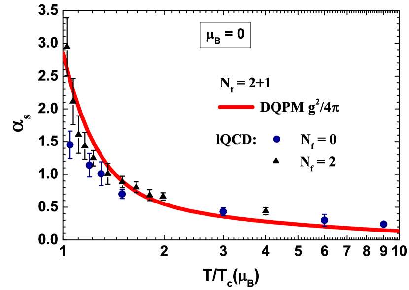
a)

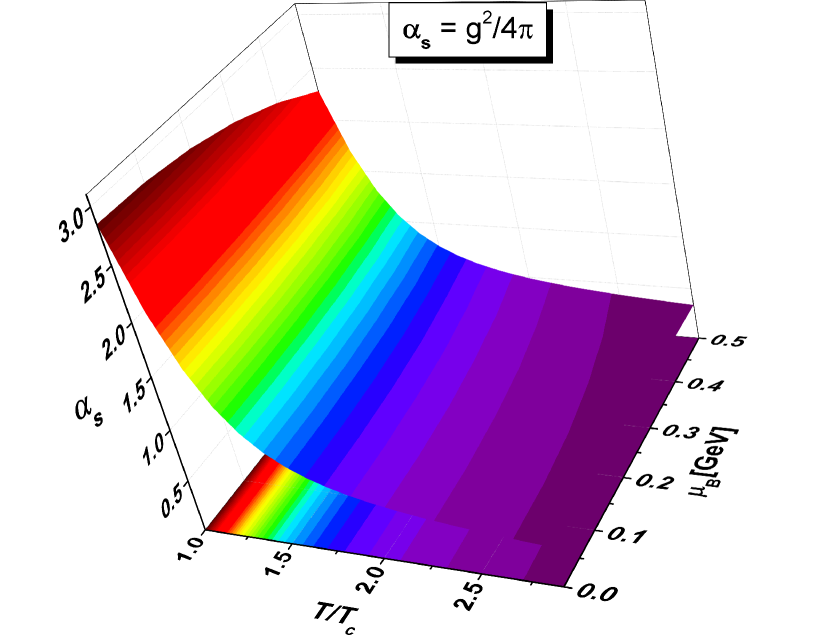
b)

Figure 9: The running coupling $\alpha_{s}=g^{2}/(4\pi)$ from the actual DQPM as a function of the scaled temperature $T/T_{c}$ at $\mu_{\mathrm{B}}=0$ a) and for moderate values of baryon chemical potential $\mu_{\mathrm{B}}<=0.5$ GeV (b) Soloveva et al. (2020c). The lattice results for quenched QCD, $N_{f}=0$, (blue circles) are taken from Ref. Kaczmarek et al. (2004) and for $N_{f}=2$ (black triangles) are taken from Ref. Kaczmarek and Zantow (2005).

with $T_{c}(\mu_{\mathrm{B}})=T_{c}(\mu_{\mathrm{B}}=0)\sqrt{1-\alpha\mu_{\mathrm{B}}^{2}}$, $T_{c}(\mu_{\mathrm{B}}=0)\approx 0.158$ GeV and $\alpha=0.974\ \text{GeV}^{-2}$. The $(T,\mu_{\mathrm{B}})$ behaviour of the DQPM coupling $g^{2}/(4\pi)$ is shown in Fig. 9 in Appendix V.1. At $\mu_{\mathrm{B}}=0$ one can see a good agreement between the lQCD evaluation of the QCD running coupling $\alpha_{s}=g^{2}/(4\pi)$ for $N_{f}=2$ Kaczmarek and Zantow (2005) and the DQPM running coupling.

With the coupling $g^{2}$ fixed from lQCD, one can now specify the dynamical quasi-particle mass (for gluons and quarks) which is assumed to be given by the HTL thermal mass in the asymptotic high-momentum regime by Bellac (2011); Linnyk et al. (2016b)

$$m^{2}_{g}(T,\mu_{\mathrm{B}})=\frac{g^{2}(T,\mu_{\mathrm{B}})}{6}\left(\left(N_{c}+\frac{N_{f}}{2}\right)T^{2}+\frac{N_{c}}{2}\sum_{q}\frac{\mu^{2}_{q}}{\pi^{2}}\right),$$

$$m^{2}_{q(\bar{q})}(T,\mu_{\mathrm{B}})=\frac{N^{2}_{c}-1}{8N_{c}}g^{2}(T,\mu_{\mathrm{B}})\left(T^{2}+\frac{\mu^{2}_{q}}{\pi^{2}}\right),$$ (31)

where $N_{c}=3$ the number of colors, while $N_{f}=3$ denotes the number of flavors. The strange quark has a larger bare mass which needs to be considered in its dynamical mass. Empirically we find $m_{s}(T,\mu_{\mathrm{B}})=m_{u/d}(T,\mu_{\mathrm{B}})+\Delta m$ and $\Delta m$ = 30 MeV. Furthermore, the quasi-particles in the DQPM have finite widths, which are adopted in the form Berrehrah et al. (2016b); Linnyk et al. (2016a)

$$\gamma_{i}(T,\mu_{\mathrm{B}})=\frac{1}{3}C_{i}\frac{g^{2}(T,\mu_{\mathrm{B}})T}{8\pi}\ln\left(\frac{2c_{m}}{g^{2}(T,\mu_{\mathrm{B}})}+1\right),$$ (32)

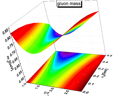
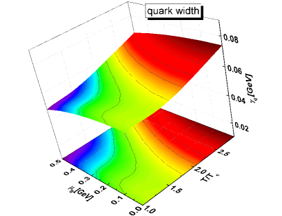
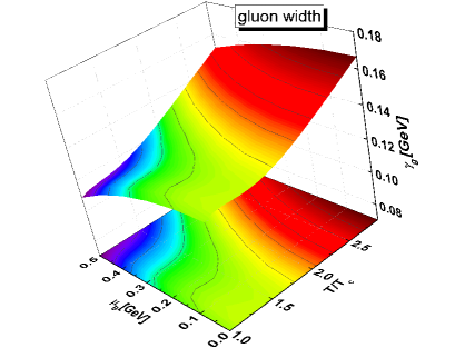
Figure 8: The effective quark (left) and gluon (right) pole-masses $M$ (upper row) and their widths $\gamma$ (lower row) from the actual DQPM as a function of the temperature $T$ and baryon chemical potential $\mu_{\mathrm{B}}$ Soloveva et al. (2020c). The strange quark mass was assumed to be $m_{s}=m_{q}+\Delta m$, with $\Delta m=30$ MeV, and the width is identical with the widths of the light quarks, $\gamma_{s}=\gamma_{q}$. In the calculation of the diffusion matrix with the Chapman-Enskog method partons were assumed to be on-shell and thus the widths vanish.

where we use the QCD color factors for quarks, $C_{q}=C_{F}=\frac{N_{c}^{2}-1}{2N_{c}}=4/3$, and gluons, $C_{g}=C_{A}=N_{c}=3$. Further, we fixed the parameter $c_{m}=14.4$, which is related to the magnetic cut-off. We assume that the width of the strange quark is the same as that for the light ($u,d$) quarks. The evaluated masses and widths in the DQPM are shown in Fig. 8 in Appendix V.1.

With the quasi-particle properties (or propagators) fixed as described above, one can evaluate the entropy density $s(T,\mu_{\mathrm{B}})$, the pressure $P_{0}(T,\mu_{\mathrm{B}})$ and energy density $\epsilon(T,\mu_{\mathrm{B}})$ in a straight forward manner by starting with the entropy density $s^{\mathrm{dqp}}$ and number density $n^{\mathrm{dqp}}$ in the propagator representation from Baym Vanderheyden and Baym (1998b); Blaizot et al. (2001) and then identifying, $s=s^{\mathrm{dqp}}$ and $n_{B}=n^{\mathrm{dqp}}/3$ Soloveva et al. (2020a). The isotropic pressure $P_{0}$ can then be obtained by using the Maxwell relation of a grand canonical ensemble:

$$P_{0}(T,\mu_{\mathrm{B}})= P_{0}(T_{0},0)+\int\limits_{T_{0}}^{T}s(T^{\prime},0)\ dT^{\prime}$$

$$+\int\limits_{0}^{\mu_{\mathrm{B}}}n_{B}(T,\mu_{\mathrm{B}}^{\prime})\ d\mu_{\mathrm{B}}^{\prime},$$ (33)

where the lower bound is chosen between $0.1<T_{0}<0.15$ GeV. The energy density $\epsilon$ then follows from the Euler relation

$$\epsilon=Ts-P+\mu_{\mathrm{B}}n_{\mathrm{B}}.$$ (34)

In Ref. Moreau et al. (2019b) we found a good agreement between the entropy density $s(T)$, pressure $P_{0}(T)$, energy density $\epsilon(T)$ and interaction measure $I(T)=\epsilon-3P$ resulting from the DQPM, and results from lQCD obtained by the BMW group Borsanyi et al. (2012, 2014) at $\mu_{\mathrm{B}}=0$ and $\mu_{\mathrm{B}}=400$ MeV.

From the above parametrizations of the masses, widths and the couplings, cross sections for anisotropic, inelastic binary tree-level QCD interactions with the dressed propagators and dressed couplings, have been evaluated which depend on temperature and baryon-chemical potential Moreau et al. (2019a); Soloveva et al. (2020a). The corresponding total cross sections are shown in Fig. 9 in Appendix V.1, and are used of in the Chapman-Enskog evaluation described in Section II.1. Further, we provide new results for the complete diffusion coefficient matrix from the DQPM in the RTA by using Eq. (27) and assuming relaxation times from Eq. (23). In the following the results from both approaches are presented.

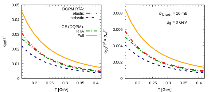
Figure 1: The scaled baryon diffusion coefficient, $\kappa_{\mathrm{BB}}/T^{2}$ (left), and the scaled electric conductivity, $\sigma_{\mathrm{el}}/T$ (right), for a partonic system with geometric cross sections, $\sigma_{\mathrm{tot}}=10$ mb at vanishing baryon-chemical potential as a function of temperature from different approaches. We compare the DQPM RTA results from Eq. (27) (for a system obeying quantum statistics, i.e. $a_{i}=\pm 1$ in Eq. (2)) with (blue dashed line) and without (red dashed-double-dotted line) inelastic, flavor-changing channels to the CE (DQPM) results either in RTA (green dashed-dotted line) from Eq. (27) (for a system obeying classical statistics, i.e. $a_{i}=0$ in Eq. (2)) or for “full” linearized collision term (orange solid line) from Eq. (18) ($a_{i}=0$ in Eq. (2)).

III Results

We provide first results for the diffusion coefficient matrix for the hot quark-gluon plasma at zero and finite baryon chemical potential $\mu_{\mathrm{B}}$ by applying the Chapman-Enskog method, reviewed in Sec. II.1 and described in detail in Refs. Greif et al. (2016, 2018); Fotakis et al. (2020), to a strongly interacting QGP system described by the DQPM (see Sec. II.3 and Ref. Soloveva et al. (2020a)). This is meant to be a significant and important improvement to the ’simplified’ model of a partonic system proposed in Refs. Greif et al. (2018); Fotakis et al. (2020). These results - obtained within the Chapman-Enskog method - are further compared to the results for the diffusion coefficient matrix calculated within RTA approach based on the DQPM as well as to various other models. The fact that the linearized Boltzmann equation is solved in the CE framework implies an improvement compared to approaches using the RTA (also see Ref. Fotakis et al. (2020)) in terms of accounting for high moments of the distribution function. However, the proposed Chapman-Enskog method requires a few approximations for the QGP description, which are not in the spirit of the DQPM, in particular:

1. The system is assumed to obey classical (Maxwell-Boltzmann) statistics (i.e. $a_{i}=0$ for all particle species in Eq. (2).

2. All particles are on-shell, therefore only the pole-masses from the DQPM, which depend on temperature and baryon-chemical potential, are assumed but their widths are neglected (for general quasiparticle properties see Appendix V.1, the Table 1 and the Fig. 8).

3. Inelastic scattering channels are neglected. That implies that flavor-changing processes are not taken into consideration, i.e. $q\bar{q}\rightarrow q^{\prime}\bar{q}^{\prime}$ are not allowed.

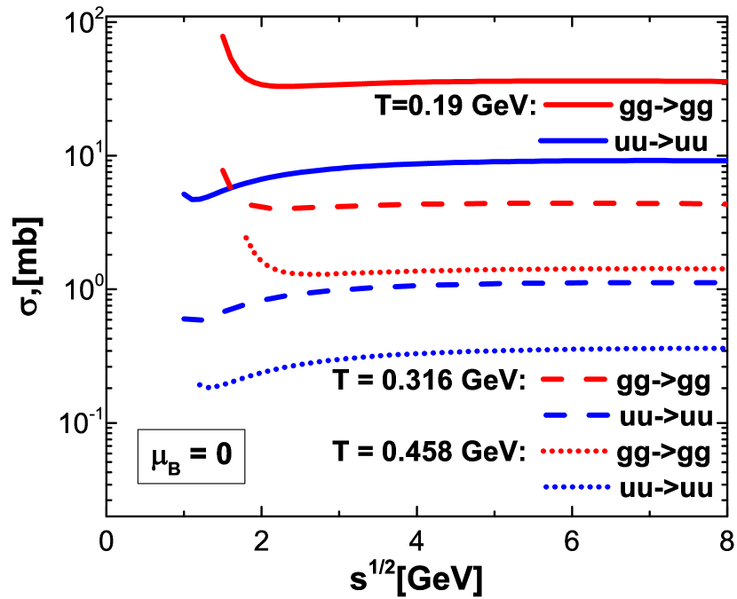
b)

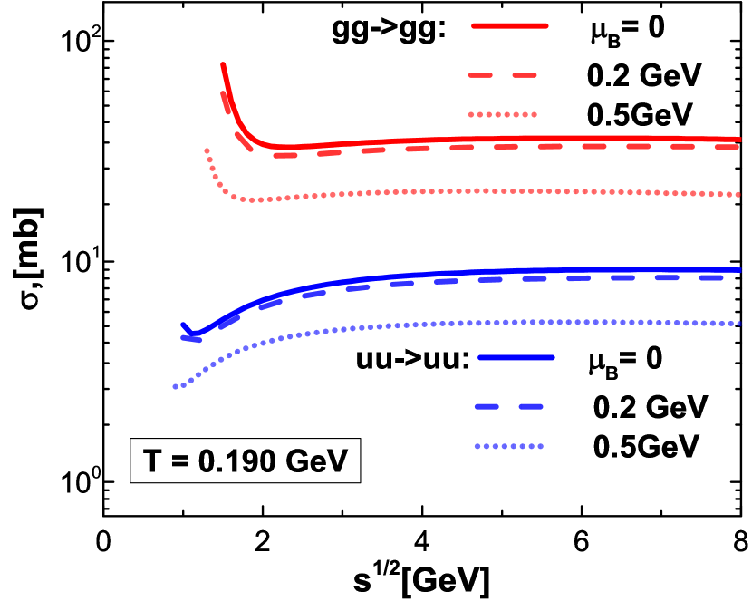
c)

Figure 10: DQPM total cross sections between different partons for the on-shell case from Eq. (11) evaluated in the center of mass of the collision system as a function of the collision energy $\sqrt{s}$ for a) $\mu_{\mathrm{B}}=0,T=0.19$ GeV for the elastic channels, b) for $\mu_{\mathrm{B}}=0,T=0.19,0.316,0.458$ GeV for both elastic and inelastic channels, and c) $\mu_{\mathrm{B}}=0,0.2,0.5$ GeV for two examples. For the minimal allowed center-of-momentum energy of the colliding partons only their pole-masses are taken into account. In the Chapman-Enskog evaluation of the diffusion matrix, the inelastic channels were neglected for simplicity.

4. All scattering processes are considered to be isotropic. We therefore feed total cross-sections into the CE evaluation which are evaluated from the anisotropic differential cross section from the DQPM via Eq. (11). The dependence on $\sqrt{s}$, temperature and baryon-chemical potential is taken into account, $\sigma^{ij\rightarrow ij}_{\mathrm{tot}}\equiv\sigma^{ij\rightarrow ij}_{\mathrm{tot}}(\sqrt{s},T,\mu_{\mathrm{B}})$ (see Appendix V.1, the Fig. 10 for an example at $\mu_{\mathrm{B}}=0$).

We note that the CE method can in principle be improved such that approximations (1) and (3) become unnecessary. In Section III.1 we find indication that approximation (3) might have a non-neglectable impact. Such improvements are left for future work. However, the nature of the method makes further improvement of points (2) and (4) difficult and require further detailed study.

The explicit manifestations of the isotropic pressure, the energy density and the net charge densities in the CE evaluation are fed with the same lattice data to which the DQPM model was fitted to (see Section II.3) as far as they are available. Since the net strangeness and net electric densities are not available from the assumed lQCD results, we compute their values from kinetic theory (see Eq. (6)).

In the following the results from the RTA approach applied to the original DQPM are denoted as “DQPM RTA” while the results from the Chapman-Enskog method applied to the DQPM under assumptions (1)-(4) (as described above) is denoted as “CE (DQPM)”. We remind here that for constant cross sections the scaled diffusion coefficients behave as $\kappa_{qq^{\prime}}/T^{2}\sim 1/T^{2}$, as found in Ref. Fotakis et al. (2020). Such a decreasing behavior is indeed found in Fig. 1.

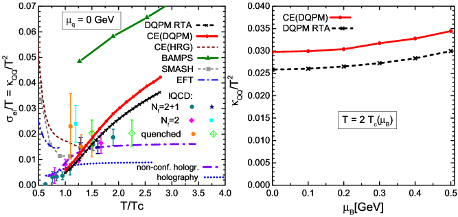
Figure 2: Left: Scaled electric conductivity, $\sigma_{\mathrm{el}}/T=\kappa_{\mathrm{QQ}}/T^{2}$, as a function of the scaled temperature $T/T_{c}$ at vanishing chemical potentials, $\mu_{q}=0$, from various approaches. The results from the CE (DQPM) is shown by the red solid line, and from DQPM RTA – by the black dashed line with crossed points. These are compared to results from the lattice QCD calculations (various shaped points with errorbars: quenched: orange circle-shaped points Ding et al. (2016), light green rhombus-shaped points Aarts et al. (2007), $N_{f}=2:$ light cyan circle-shaped points Brandt et al. (2013), magenta rhombus-shaped points Brandt et al. (2016), and $N_{f}=2+1:$ dark cyan circle-shaped points Aarts et al. (2015) and blue stars Astrakhantsev et al. (2020)), the kinetic partonic cascade model BAMPS (dark-green solid line with triangular-shaped points) Greif et al. (2014), and from conformal Rougemont et al. (2015) (blue dotted line) and non-conformal Finazzo and Noronha (2014) (violet dashed-dotted line) holographic models. For temperatures below $T_{c}=0.158$ GeV we show evaluations from hadronic models: SMASH Weil et al. (2016); Hammelmann et al. (2019); Rose et al. (2020) (grey short-dashed line with squared points), effective field theory (EFT) Torres-Rincon (2012) (blue dashed-dotted line), and CE tuned to a hadron gas [CE (HRG)] from Refs. Greif et al. (2016, 2018); Fotakis et al. (2020) (dark-red dashed line). Right: Scaled electric conductivity of the QGP at fixed scaled temperature, $T=2T_{c}(\mu_{\mathrm{B}})$, and vanishing $\mu_{\mathrm{Q}}$ and $\mu_{\mathrm{S}}$ are shown for varying baryon chemical potential $\mu_{\mathrm{B}}$ from the DQPM RTA (black dashed line with cross-shaped points) and the CE (DQPM) (red solid line with circle-shaped points) evaluation.

III.1 Model study: constant isotropic cross sections

In order to evaluate the systematic differences between the DQPM RTA and the CE (DQPM) approaches we perform a here ’model study’ by assuming a (total) geometric cross section of $\sigma_{\mathrm{tot}}=10$ mb for all interactions. For this comparison we consider the same assumptions as described in the preface above, but assume all channels to be characterized by the constant cross section.

In Fig. 1 we show results for the scaled baryon coefficient, $\kappa_{\mathrm{BB}}/T^{2}$ (left plot), and the scaled electric conductivity, $\sigma_{\mathrm{el}}/T$ (right plot) at $\mu_{\mathrm{B}}=0$ in a temperature range from 160 MeV to 420 MeV. The DQPM RTA calculations are presented for two cases: firstly, where all binary channels, including the inelastic ones, are considered (blue dashed line), and for the case where only the elastic channels are accounted for (red dashed-double-dotted line). For the DQPM RTA results presented in this paper we use Eq. (27) (for a system obeying quantum statistics, i.e. $a_{i}=\pm 1$ in Eq. (2)). The CE (DQPM) calculations are presented in Fig. 1 also for two cases: in the first case we evaluate the coefficients in RTA with the help of Eq. (27) (for a system obeying classical statistics, i.e. $a_{i}=0$ in Eq. (2) ) under the assumption of the simplistic relaxation time, $\tau_{0}=1/{n_{\mathrm{tot}}\bar{\sigma}_{T}}$ (orange solid line), and for the second case we consider the full linearized Boltzmann equation via Eq. (18) (for a system obeying classical statistics, i.e. $a_{i}=0$ in Eq. (2) ) (green dashed-dotted line).

This ’model study’ shows the influence of the consideration of the linearized Boltzmann equation compared to its relaxation time approximation, and the influence of the inelastic channels compared to its neglection. We find that the consideration of the full linearized collision term effectively reduces the scattering rate of a specific particle species, while in the RTA the scattering rate is overestimated. This is because in the collision term not only the scattering of particles from a specific momentum bin into all other disjoint momentum bins is considered, but also the rescattering into this particular momentum bin is accounted for (gain and loss term). As argued in Ref. Fotakis et al. (2020) such an overestimation of the scattering rate leads to a decrease of the diffusion coefficients from RTA (which are anti-proportional to the rate).

Furthermore, we find that the inelastic channels lead to a further decrease of the diffusion coefficients due to the repeated effective increase of the scattering rate as shown in Fig. 1. Comparing the elastic version of the DQPM RTA evaluation with the CE (DQPM) calculation in the RTA limit (Eq. (27)), we find a good agreement of the results at high temperatures. This is expected since the only difference between both calculations – DQPM RTA and CE (DQPM) in the RTA limit – is the consideration of quantum corrections and the more sophisticated (momentum-dependent) relaxation time in DQPM RTA.

III.2 Diffusion coefficient matrix of the quark-gluon plasma

In the following we show results for the scaled diffusion coefficient matrix, $\kappa_{qq^{\prime}}/T^{2}$, for the partonic phase from the DQPM (RTA) and CE (DQPM) evaluation under the considerations described in the preface of Section III. Additionally we consider two cases:

• We fix all chemical potentials to zero, $\mu_{q}=0$ ($q=\mathrm{B},\mathrm{S},\mathrm{Q}$), and show the temperature dependence of the coefficients.

• We fix the temperature to $T=2T_{c}(\mu_{\mathrm{B}})$, and show their dependence on the baryon chemical potential, $\mu_{\mathrm{B}}$. Here we further set the other chemical potentials to zero, $\mu_{\mathrm{S}}=0$ and $\mu_{\mathrm{Q}}=0$.

For most coefficients we find a rich $\mu_{\mathrm{B}}$-dependence. This dependence originates from the fact that all quarks carry baryon number and thus are sensitive to variations in $\mu_{\mathrm{B}}$. In Ref. Fotakis et al. (2020) the temperature dependence of these transport coefficients was reviewed, and it was found that they roughly scale as $\kappa_{qq^{\prime}}/T^{2}\sim 1/(\sigma_{\mathrm{tot}}T^{2})$. In the case of the DQPM at fixed chemical potential, the cross sections depend on temperature as $\sigma_{\mathrm{tot}}\sim 1/T^{3}$ or $\sim 1/T^{4}$ (for the considered temperature range). This depends on the combinations of $s-,t-,u-$ channels for different parton-parton scatterings: for $q-q$, $q-\bar{q}$ and $q-g$ scatterings $\sigma_{\mathrm{tot}}\sim 1/T^{3}$, while for the $g-g$ channel the terms $1/T^{3}$, $1/T^{4}$ have equivalent contribution to the total cross-section $\sigma_{\mathrm{tot}}\sim c_{3}/T^{3}+c_{4}/T^{4}$, where $c_{3},c_{4}$ depend on $\sqrt{s},\mu_{\mathrm{B}}$ (see e.g. Fig. 10 in Appendix V.1). The temperature dependence of the cross-sections is in accordance with the temperature scaling of the DQPM coupling constant $g^{2}(T,\mu_{\mathrm{B}})$ (see e.g. Fig. 9 in Appendix V.1 ). This leads to a roughly quadratic dependence in temperature, $\kappa_{qq^{\prime}}/T^{2}\sim T^{2}$, which is demonstrated in the figures below.

We remind that the diffusion coefficient matrix is symmetric and therefore we may only show six instead of nine coefficients Onsager (1931a, b). In the following we subdivide the presentation of the conductivities in three sections: electric conductivities ($\kappa_{\mathrm{QQ}}$, $\kappa_{\mathrm{QS}}$ and $\kappa_{\mathrm{QB}}$), strange conductivities ($\kappa_{\mathrm{SS}}$ and $\kappa_{\mathrm{SB}}$), and finally the baryon conductivities ($\kappa_{\mathrm{BB}}$). Since diffusion coefficients and conductivities are related to each other via temperature, $\kappa_{qq^{\prime}}=\sigma_{qq^{\prime}}T$, we use their denomination interchangeably.

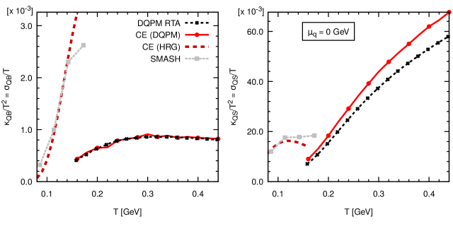
Figure 3: Scaled cross-electric conductivities, $\sigma_{\mathrm{QB}}/T^{2}$ (left) and $\sigma_{\mathrm{QS}}/T^{2}$ (right), from SMASH Weil et al. (2016); Rose et al. (2020) (grey short-dashed line with square-shaped points), the DQPM RTA (black dashed line with cross-shaped points), and the CE (DQPM) (red solid line with circle-shaped points) and CE (HRG) Greif et al. (2018); Fotakis et al. (2020) (dark-red dashed line) evaluation at vanishing chemical potentials, $\mu_{q}=0$, for temperatures between 80 and 420 MeV.

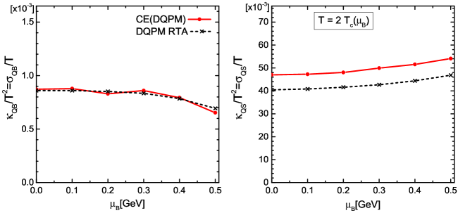
Figure 4: Scaled cross-electric conductivities, $\sigma_{\mathrm{QB}}/T^{2}$ (left) and $\sigma_{\mathrm{QS}}/T^{2}$ (right), from the DQPM RTA (black dashed line with cross-shaped points) and the CE (DQPM) evaluation at fixed scaled temperature, $T=2T_{c}(\mu_{\mathrm{B}})$, shown over baryon chemical potential $\mu_{\mathrm{B}}$ in range 0 to 0.5 GeV. Further, the other chemical potentials are fixed to zero, $\mu_{\mathrm{Q}}=0$ and $\mu_{\mathrm{S}}=0$.

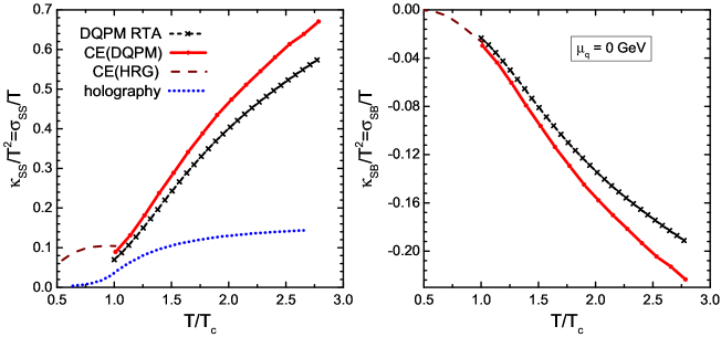
Figure 5: Scaled strange and strange-baryon diffusion coefficients, $\kappa_{\mathrm{SS}}/T^{2}$ (left) and $\kappa_{\mathrm{SB}}/T^{2}$ (right), as a function of scaled temperature in the range from 0.5 to 3 $T_{c}$ at vanishing chemical potentials, $\mu_{q}=0$. We compare results from CE (DQPM) (red solid line with circles), DQPM RTA (black dashed-line with crossed-shaped points), the CE (HRG) Greif et al. (2018); Fotakis et al. (2020) (dark-red dashed line) and from conformal holography Rougemont et al. (2015) (blue dotted line).

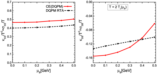
Figure 6: Scaled strange and strange-baryon diffusion coefficients, $\kappa_{\mathrm{SS}}/T^{2}$ (left) and $\kappa_{\mathrm{SB}}/T^{2}$ (right), from the DQPM RTA (black dashed line with cross-shaped points) and the CE (DQPM) evaluation at fixed scaled temperature, $T=2T_{c}(\mu_{\mathrm{B}})$, shown over baryon chemical potential $\mu_{\mathrm{B}}$ in range 0 to 0.5 GeV. Further, the other chemical potentials are fixed to zero, $\mu_{\mathrm{Q}}=0$ and $\mu_{\mathrm{S}}=0$.

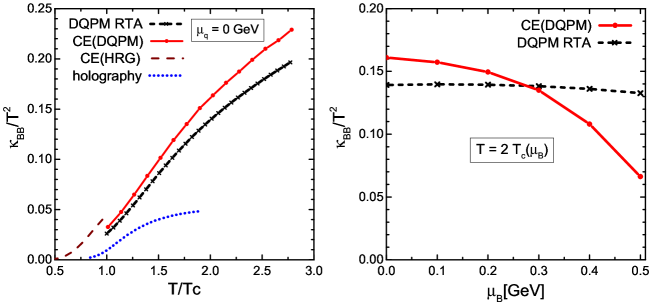
Figure 7: Scaled baryon diffusion coefficient, $\kappa_{\mathrm{BB}}/T^{2}$, (left) at vanishing chemical potentials, $\mu_{q}=0$, as a function of the scaled temperature from various approaches and (right) at fixed scaled temperature, $T=2T_{c}(\mu_{\mathrm{B}})$, as a function of baryon chemical potential $\mu_{\mathrm{B}}$. The strange and electric potential are fixed to zero: $\mu_{\mathrm{S}}=0$ and $\mu_{\mathrm{Q}}=0$. We show results from the CE evaluation tuned to DQPM (red solid line), as described above, and tuned to a hadron gas from Refs. Greif et al. (2018); Fotakis et al. (2020) (dark-red dashed line). We again compare to the calculation from DQPM RTA Soloveva et al. (2020a) (black dashed line with crosses) and to conformal holography Rougemont et al. (2015) (blue dotted line) as done for the electric conductivity.

III.2.1 Electric conductivities

The electric conductivity, $\sigma_{\mathrm{el}}/T$, was evaluated in various models (cf. Refs. Arnold et al. (2000); Brandt et al. (2013); Torres-Rincon (2012); Finazzo and Noronha (2014); Amato et al. (2013); Marty et al. (2013); Aarts et al. (2015); Greif et al. (2014); Puglisi et al. (2014, 2015); Brandt et al. (2016); Rougemont et al. (2015); Ding et al. (2016); Greif et al. (2016); Berrehrah et al. (2016b); Thakur et al. (2017); Rougemont et al. (2017); Greif et al. (2018); Hammelmann et al. (2019); Soloveva et al. (2020a); Fotakis et al. (2020); Rose et al. (2020)). In Fig. 2 we compare the results from DQPM RTA and CE (DQPM) to a variety of models for both, the partonic Brandt et al. (2013); Amato et al. (2013); Aarts et al. (2015); Greif et al. (2014); Rougemont et al. (2015); Finazzo and Noronha (2014) and hadronic phase Hammelmann et al. (2019); Rose et al. (2020); Torres-Rincon (2012); Greif et al. (2016, 2018); Fotakis et al. (2020), at $\mu_{\mathrm{q}}=0$ in a temperature range between 0 and 3$\,T_{c}$, where here the deconfinement temperature is $T_{c}=158$ MeV. The Chapman-Enskog and RTA results for the dimensionless ratio of electric conductivity to temperature $\sigma_{\mathrm{el}}/T$ (later referred to as scaled electric conductivity) for $\mu_{q}=0$ are presented in Fig.2 (left) as solid red and dashed black lines. Results for both methods have a similar increase with temperature, which is mainly a consequence of the temperature dependence of the cross section (as discussed before) and also of the increasing total electric charge density Fotakis et al. (2020).

We find that the results from DQPM RTA and CE (DQPM) are consistent with results from lattice QCD in the vicinity of the crossover region, $1\leq T/T_{c}\leq 1.5$. We again point out the apparent quadratic dependence on temperature which was shortly motivated in the preface of this section above. Due to our discussion from Section III.1 we suppose that a realistic result for the conductivities may be between the evaluations from DQPM RTA and CE (DQPM).

As follows from Fig. 2, the hadronic models presented there – the hadronic transport model SMASH Weil et al. (2016); Hammelmann et al. (2019); Rose et al. (2020) (grey short-dashed line with squared points), effective field theory (EFT) Torres-Rincon (2012) (blue dashed-dotted line), and CE tuned to a hadron gas [CE (HRG)] from Refs. Greif et al. (2016, 2018); Fotakis et al. (2020) (dark-red dashed line) – substantially overestimate the lQCD data in the vicinity of $T_{c}$ as well as the results from the conformal Rougemont et al. (2015) (blue dotted line) and non-conformal Finazzo and Noronha (2014) (violet dashed-dotted line) holographic models. The DQPM RTA results are in a good agreement in the vicinity of phase transition with the previous estimations for DQPM* from Ref. Berrehrah et al. (2016b), where non-relativistic formula for estimation the electric conductivity was used, which results in the linear dependence of the $\sigma_{el}/T$ on temperature while presented DQPM results show the quadratic dependence on temperature.

Additionally to the electric conductivity, in Fig. 3 we show the cross-electric conductivities, $\sigma_{\mathrm{BQ}}$ and $\sigma_{\mathrm{QS}}$, from the CE (DQPM) and the DQPM RTA calculation together with results achieved within SMASH Rose et al. (2020) and the CE (HRG) evaluation from Refs. Greif et al. (2018); Fotakis et al. (2020) for the same thermal considerations for the hadronic phase. Comparing the results in both phases, we find a significant disagreement for $\sigma_{QB}$ around the crossover temperature. Further, we find such discrepancies to a smaller extend in the other electric conductivities and in the coefficients to follow. Such disagreement may hint to a difference in the chemical composition of the adjacent phases Rose et al. (2020).

Furthermore, as advertized in the preface, in Figs. 2 (right) and 4 we present the sensitivity of the electric conductivities on $\mu_{\mathrm{B}}$ at fixed scaled temperature, $T=2T_{c}(\mu_{\mathrm{B}})$. Compared to the coefficients directly connected to the baryonic sector, we find a rather weak dependence on $\mu_{\mathrm{B}}$ (see discussion of $\kappa_{\mathrm{BB}}$ and $\kappa_{\mathrm{SB}}$). Surprisingly also $\sigma_{\mathrm{QB}}$ has such a weak dependence even though it also belongs to the baryonic sector. Further, $\sigma_{\mathrm{QB}}$ is very small - it has the smallest magnitude of all conductivities in the diffusion matrix. One can discuss its plausibility with a symmetry argument: the $\sigma_{\mathrm{QB}}$ coefficient relates the generated electric current to the baryonic gradient which generates it (via the corresponding Navier-Stokes term). Assume a QGP with constant geometric cross section as discussed in Section III.1. Further, assume that all quarks have the same mass. The down- and strange-quark have the same baryon number and electric charge, $\mathrm{B}=+1/3$ and $\mathrm{Q}=-1/3e$, while the up-quark has $\mathrm{B}=+1/3$ and $\mathrm{Q}=+2/3e$, i.e. the same baryon number but an electric charge which is twice the magnitude but has the opposite sign (refer to Table 1). Due to the quarks carrying the same baryon number, a baryon gradient generates a baryon current $V^{\mu}_{\mathrm{B}}$ which is equally composed by a current of up-, down- and strange-quarks ($V_{i}^{\mu}$): $V^{\mu}_{\mathrm{B}}=\sum_{i}\mathrm{B}_{i}V^{\mu}_{i}$, with $V^{\mu}_{i}=V^{\mu}_{\mathrm{quark}}$ $\forall i$. With this we can estimate the generated electric current:

$$V^{\mu}_{\mathrm{Q}}=\sum_{i}\mathrm{Q}_{i}V^{\mu}_{i}=V^{\mu}_{\mathrm{quark}}\left(-\frac{1}{3}-\frac{1}{3}+\frac{2}{3}\right)=0.$$ (35)

The same argument can be made additionally accounting for the anti-quarks. The non-equal mass of the quarks and the varying cross sections lead to a non-vanishing $\sigma_{\mathrm{QB}}$. However, the above estimate illustrate the small magnitude of the respected coefficient.

III.2.2 Strange conductivities

We continue with the results for the strange sector: $\kappa_{\mathrm{SS}}$ and $\kappa_{\mathrm{SB}}$. The coefficient $\kappa_{\mathrm{SQ}}$, or equivalently $\sigma_{\mathrm{SQ}}=\sigma_{\mathrm{QS}}$, was already discussed above as part of the electric sector. Fig. 5 shows the $\kappa_{\mathrm{SS}}$ and $\kappa_{\mathrm{SB}}$ as a function of temperature at vanishing chemical potentials. Further, we show their $\mu_{\mathrm{B}}$-dependence in Fig. 6 in the range $\mu_{\mathrm{B}}=0$ to 0.5 GeV at fixed scaled temperature, $T=2T_{c}(\mu_{\mathrm{B}})$ and for vanishing electric and strange chemical potential. We compare results from the DQPM RTA and CE (DQPM) computation to results from CE (HRG) in our recent publications Greif et al. (2018); Fotakis et al. (2020), and to results from conformal holography Rougemont et al. (2015).

We find that the baryon-strange diffusion coefficient is negative due to the definition of strangeness carried by the s-quark as has been already advocated in Ref. Greif et al. (2018); Fotakis et al. (2020). We obtain an almost quadratic dependence in temperature again, and a rather strong dependency on $\mu_{\mathrm{B}}$. However, the results from DQPM RTA for $\kappa_{\mathrm{SB}}$ in Fig. 6 show a slightly different $\mu_{\mathrm{B}}$-behavior than the results from CE (DQPM) for $\mu_{\mathrm{B}}\geq 0.3$ GeV. Furthermore, judging from Fig. 5, in the vicinity of the crossover region the results from CE (HRG) for the hadronic phase, and the calculation from the DQPM RTA and CE (DQPM) agree well. As for other diffusion coefficients, the scaled strange diffusion coefficient from holography has a different temperature dependence and smaller values in the vicinity of the crossover phase transition.

III.2.3 Baryon conductivities

In order to describe the deconfined QCD medium at the non-zero baryon density one should first consider the baryon diffusion coefficient $\kappa_{\mathrm{BB}}$. This diffusion coefficient was already evaluated in various models Arnold et al. (2003); Rougemont et al. (2015); Greif et al. (2018); Ghiglieri et al. (2018); Fotakis et al. (2020); Soloveva et al. (2020a). Fig. 7 (left) shows the temperature dependence of the baryon diffusion coefficient for the quark-gluon plasma estimated with the CE (DQPM) (red solid line) and DQPM RTA approaches (black dashed line with crosses). We also show the results from conformal holography Rougemont et al. (2015) (blue dotted lines). For temperatures below $T_{c}$ we again refer to the CE (HRG) calculation from Refs. Greif et al. (2018); Fotakis et al. (2020) (dark-red dashed line). The comparison is presented at zero chemical potentials $\mu_{q}=0$. Around $T_{c}$ the results from DQPM RTA, CE (DQPM) and CE (HRG) seem to be rather consistent with each other. Furthermore, we show its dependence on $\mu_{\mathrm{B}}$ at fixed scaled temperature $T=2T_{c}(\mu_{\mathrm{B}})$ in Fig. 7 (right). The DQPM RTA shows a rather weak $\mu_{\mathrm{B}}$ dependence, while $\kappa_{\mathrm{BB}}$ from the CE (DQPM) decreases with $\mu_{\mathrm{B}}$.

IV Conclusion

In this study we have calculated the complete diffusion coefficient matrix $\kappa_{qq^{\prime}}$ ($q,q^{\prime}=\mathrm{B},\mathrm{S},\mathrm{Q}$) of the strongly interacting quark-gluon plasma by using the Chapman-Enskog method as well as the relaxation time approximation (RTA) from kinetic theory. We have explored the $T$ and $\mu_{\mathrm{B}}$ dependencies of the diffusion coefficients by considering microscopical properties of quarks and gluons within the dynamical quasi-particle model (DQPM). The DQPM predictions of thermodynamic quantities for finite $\mu_{\mathrm{B}}$ show a good agreement with the available lQCD EoS Moreau et al. (2019b). Moreover, for $\mu_{\mathrm{B}}=0$ the DQPM estimations of the QGP electric conductivity ($\sigma_{el}/T^{2}$) are in a good agreement with the $N_{f}=2+1$ lQCD results and in case of the specific shear and bulk viscosities ($\eta/s,\ \zeta/s$) the estimations are remarkably close to the predictions from the gluodynamic lQCD calculations Soloveva et al. (2020a).
We find that the electric conductivities ($\kappa_{\mathrm{QQ}}$, $\kappa_{\mathrm{QS}}$ and $\kappa_{\mathrm{QB}}$), strange conductivities ($\kappa_{\mathrm{SS}}$ and $\kappa_{\mathrm{SB}}$), and finally the baryon conductivity ($\kappa_{\mathrm{BB}}$) have a similar temperature dependence in the vicinity of the phase transition while the $\mu_{\mathrm{B}}$ dependence is rather different among the considered diffusion coefficients. In particular, the diffusion coefficients $\kappa_{\mathrm{BB}}$ and $\kappa_{\mathrm{QB}}$ decrease with $\mu_{\mathrm{B}}$, while other coefficients increase. A suppression of baryon diffusion in a sQGP with finite $\mu_{\mathrm{B}}$ has been seen also in the holographic calculations Rougemont et al. (2015).

One of the main endeavors of this paper is to deliver reasonable estimates for the diffusion coefficients of the strongly interacting quark-gluon plasma. Furthermore, we compare the RTA evaluations from recent DQPM publications Soloveva et al. (2020a, c, b) with the Chapman-Enskog method. We demonstrate that once the cross sections and the (thermal) properties (masses, equation of state, etc.) of a system are known, the CE framework at hand is able to deliver consistent results. We show a good agreement for both methods with the available predictions from the literature for the partonic phase, in particular results for the scaled electric conductivity are remarkably close to the lQCD estimates at $\mu_{\mathrm{B}}=0$, as well as with the estimates for the hadronic phase. However, $\kappa_{QB}$ non-diagonal diffusion coefficient doesn’t coincide well in the vicinity of the phase transition with the estimates for the hadronic phase, which can be interpreted as an indication of a difference in the chemical composition of the adjacent phases. There are several model calculations of diagonal conductivities (mostly $\kappa_{\mathrm{QQ}}$) in the literature that are similar to the RTA approach but used numerous restrictive assumptions for the evaluation of the relaxation times or cross-sections. Studying the diffusion coefficients of the QGP should have future benefits when considering hydrodynamical description for the time evolution of the deconfined QCD medium.

V Appendix

V.1 Properties of partons in the DQPM

Name	Spin	Degeneracy	Baryon	Electric	Strangeness
			Number	Charge
$g$	$1$	$16$	$0$	$0$	$0$
$u$	$1/2$	$6$	$+1/3$	$+2/3e$	$0$
$\bar{u}$	$1/2$	$6$	$-1/3$	$-2/3e$	$0$
$d$	$1/2$	$6$	$+1/3$	$-1/3e$	$0$
$\bar{d}$	$1/2$	$6$	$-1/3$	$+1/3e$	$0$
$s$	$1/2$	$6$	$+1/3$	$-1/3e$	$-1$
$\bar{s}$	$1/2$	$6$	$-1/3$	$+1/3e$	$+1$

Table 1: Properties of the particle species considered in the quark-gluon plasma in this work. Here, $e$ denotes the elementary electric charge in natural units.

a)

References

- Ollitrault (1992) J.-Y. Ollitrault, Phys. Rev. D 46, 229 (1992).
- Heinz and Kolb (2002) U. W. Heinz and P. F. Kolb, Nucl. Phys. A 702, 269 (2002), arXiv:hep-ph/0111075 .
- Shuryak (2009) E. Shuryak, Prog. Part. Nucl. Phys. 62, 48 (2009), arXiv:0807.3033 [hep-ph] .
- Shuryak (2005) E. V. Shuryak, Nucl. Phys. A 750, 64 (2005), arXiv:hep-ph/0405066 .
- Gyulassy and McLerran (2005) M. Gyulassy and L. McLerran, Nucl. Phys. A 750, 30 (2005), arXiv:nucl-th/0405013 .
- Romatschke and Romatschke (2007) P. Romatschke and U. Romatschke, Phys. Rev. Lett. 99, 172301 (2007), arXiv:0706.1522 [nucl-th] .
- Cheng et al. (2008) M. Cheng et al., Phys. Rev. D 77, 014511 (2008), arXiv:0710.0354 [hep-lat] .
- Aoki et al. (2009) Y. Aoki, S. Borsanyi, S. Durr, Z. Fodor, S. D. Katz, S. Krieg, and K. K. Szabo, JHEP 06, 088 (2009), arXiv:0903.4155 [hep-lat] .
- Denicol et al. (2018) G. S. Denicol, C. Gale, S. Jeon, A. Monnai, B. Schenke, and C. Shen, Phys. Rev. C98, 034916 (2018), arXiv:1804.10557 .
- Li and Shen (2018) M. Li and C. Shen, Phys. Rev. C98, 064908 (2018), arXiv:1809.04034 .
- Du and Heinz (2019) L. Du and U. Heinz, (2019), 10.1016/j.cpc.2019.107090, arXiv:1906.11181 [nucl-th] .
- Arnold et al. (2003) P. B. Arnold, G. D. Moore, and L. G. Yaffe, JHEP 05, 051 (2003), arXiv:hep-ph/0302165 [hep-ph] .
- Rougemont et al. (2015) R. Rougemont, J. Noronha, and J. Noronha-Hostler, Phys. Rev. Lett. 115, 202301 (2015), arXiv:1507.06972 .
- Greif et al. (2018) M. Greif, J. A. Fotakis, G. S. Denicol, and C. Greiner, Phys. Rev. Lett. 120, 242301 (2018), arXiv:1711.08680 .
- Ghiglieri et al. (2018) J. Ghiglieri, G. D. Moore, and D. Teaney, JHEP 03, 179 (2018), arXiv:1802.09535 [hep-ph] .
- Fotakis et al. (2020) J. A. Fotakis, M. Greif, C. Greiner, G. S. Denicol, and H. Niemi, Phys. Rev. D 101, 076007 (2020), arXiv:1912.09103 [hep-ph] .
- Soloveva et al. (2020a) O. Soloveva, P. Moreau, and E. Bratkovskaya, Phys. Rev. C 101, 045203 (2020a).
- Rose et al. (2020) J.-B. Rose, M. Greif, J. Hammelmann, J. A. Fotakis, G. S. Denicol, H. Elfner, and C. Greiner, Phys. Rev. D 101, 114028 (2020), arXiv:2001.10606 [nucl-th] .
- Turbide et al. (2004) S. Turbide, R. Rapp, and C. Gale, Phys. Rev. C 69, 014903 (2004).
- Akamatsu et al. (2011) Y. Akamatsu, H. Hamagaki, T. Hatsuda, and T. Hirano, Journal of Physics G: Nuclear and Particle Physics 38, 124184 (2011).
- Linnyk et al. (2016a) O. Linnyk, E. L. Bratkovskaya, and W. Cassing, Prog. Part. Nucl. Phys. 87, 50 (2016a), arXiv:1512.08126 [nucl-th] .
- Yin (2014) Y. Yin, Phys. Rev. C 90, 044903 (2014).
- Tuchin (2013) K. Tuchin, Phys. Rev. C 88, 024911 (2013).
- Inghirami et al. (2019) G. Inghirami, M. Mace, Y. Hirono, L. Del Zanna, D. E. Kharzeev, and M. Bleicher, (2019), arXiv:1908.07605 [hep-ph] .
- Denicol et al. (2019) G. S. Denicol, E. Molnár, H. Niemi, and D. H. Rischke, Phys. Rev. D 99, 056017 (2019), arXiv:1902.01699 [nucl-th] .
- Oliva (2020) L. Oliva, Eur. Phys. J. A 56, 255 (2020), arXiv:2007.00560 [nucl-th] .
- Arnold et al. (2000) P. B. Arnold, G. D. Moore, and L. G. Yaffe, JHEP 11, 001 (2000), arXiv:hep-ph/0010177 .
- Brandt et al. (2013) B. B. Brandt, A. Francis, H. B. Meyer, and H. Wittig, JHEP 03, 100 (2013), arXiv:1212.4200 [hep-lat] .
- Torres-Rincon (2012) J. M. Torres-Rincon, Hadronic Transport Coefficients from Effective Field Theories, Ph.D. thesis, UCM, Somosaguas, New York (2012), arXiv:1205.0782 .
- Finazzo and Noronha (2014) S. I. Finazzo and J. Noronha, Phys. Rev. D 89, 106008 (2014), arXiv:1311.6675 [hep-th] .
- Amato et al. (2013) A. Amato, G. Aarts, C. Allton, P. Giudice, S. Hands, and J.-I. Skullerud, Phys. Rev. Lett. 111, 172001 (2013), arXiv:1307.6763 [hep-lat] .
- Marty et al. (2013) R. Marty, E. Bratkovskaya, W. Cassing, J. Aichelin, and H. Berrehrah, Phys. Rev. C 88, 045204 (2013).
- Aarts et al. (2015) G. Aarts, C. Allton, A. Amato, P. Giudice, S. Hands, and J.-I. Skullerud, JHEP 02, 186 (2015), arXiv:1412.6411 .
- Greif et al. (2014) M. Greif, I. Bouras, C. Greiner, and Z. Xu, Phys. Rev. D90, 094014 (2014), arXiv:1408.7049 .
- Puglisi et al. (2014) A. Puglisi, S. Plumari, and V. Greco, Phys. Rev. D90, 114009 (2014), arXiv:1408.7043 .
- Puglisi et al. (2015) A. Puglisi, S. Plumari, and V. Greco, Physics Letters B 751, 326 (2015).
- Brandt et al. (2016) B. B. Brandt, A. Francis, B. Jaeger, and H. B. Meyer, Phys. Rev. D93, 054510 (2016), arXiv:1512.07249 .
- Ding et al. (2016) H.-T. Ding, O. Kaczmarek, and F. Meyer, Phys. Rev. D94, 034504 (2016), arXiv:1604.06712 .
- Greif et al. (2016) M. Greif, C. Greiner, and G. S. Denicol, Phys. Rev. D93, 096012 (2016), [Erratum: Phys. Rev.D96, 059902 (2017)], arXiv:1602.05085 .
- Thakur et al. (2017) L. Thakur, P. K. Srivastava, G. P. Kadam, M. George, and H. Mishra, Phys. Rev. D 95, 096009 (2017).
- Rougemont et al. (2017) R. Rougemont, R. Critelli, J. Noronha-Hostler, J. Noronha, and C. Ratti, Phys. Rev. D96, 014032 (2017), arXiv:1704.05558 .
- Hammelmann et al. (2019) J. Hammelmann, J. M. Torres-Rincon, J.-B. Rose, M. Greif, and H. Elfner, Phys. Rev. D99, 076015 (2019), arXiv:1810.12527 [hep-ph] .
- Peshier and Cassing (2005) A. Peshier and W. Cassing, Phys. Rev. Lett. 94, 172301 (2005), arXiv:hep-ph/0502138 [hep-ph] .
- Cassing (2007a) W. Cassing, Nucl. Phys. A795, 70 (2007a), arXiv:0707.3033 [nucl-th] .
- Cassing (2007b) W. Cassing, Nucl. Phys. A 791, 365 (2007b), arXiv:0704.1410 [nucl-th] .
- Linnyk et al. (2016b) O. Linnyk, E. Bratkovskaya, and W. Cassing, Prog. Part. Nucl. Phys. 87, 50 (2016b), arXiv:1512.08126 [nucl-th] .
- Berrehrah et al. (2016a) H. Berrehrah, E. Bratkovskaya, T. Steinert, and W. Cassing, Int. J. Mod. Phys. E 25, 1642003 (2016a), arXiv:1605.02371 [hep-ph] .
- Kaczmarek et al. (2004) O. Kaczmarek, F. Karsch, F. Zantow, and P. Petreczky, Phys. Rev. D70, 074505 (2004), [Erratum: Phys. Rev.D72,059903(2005)], arXiv:hep-lat/0406036 [hep-lat] .
- Moreau et al. (2019a) P. Moreau, O. Soloveva, L. Oliva, T. Song, W. Cassing, and E. Bratkovskaya, Phys. Rev. C 100, 014911 (2019a), arXiv:1903.10257 [nucl-th] .
- Vanderheyden and Baym (1998a) B. Vanderheyden and G. Baym, J. Statist. Phys. 93, 843 (1998a), arXiv:hep-ph/9803300 .
- Kadanoff and Baym (1962) L. Kadanoff and G. Baym, Benjamin, New York , 203 pp (1962).
- Cassing and Bratkovskaya (2008) W. Cassing and E. Bratkovskaya, Phys. Rev. C 78, 034919 (2008), arXiv:0808.0022 [hep-ph] .
- Cassing (2009) W. Cassing, Eur. Phys. J. ST 168, 3 (2009), arXiv:0808.0715 [nucl-th] .
- Cassing and Bratkovskaya (2009) W. Cassing and E. Bratkovskaya, Nucl. Phys. A 831, 215 (2009), arXiv:0907.5331 [nucl-th] .
- Bratkovskaya et al. (2011) E. Bratkovskaya, W. Cassing, V. Konchakovski, and O. Linnyk, Nucl. Phys. A 856, 162 (2011), arXiv:1101.5793 [nucl-th] .
- Ozvenchuk et al. (2013) V. Ozvenchuk, O. Linnyk, M. Gorenstein, E. Bratkovskaya, and W. Cassing, Phys. Rev. C 87, 024901 (2013), arXiv:1203.4734 [nucl-th] .
- Soloveva et al. (2020b) O. Soloveva, P. Moreau, L. Oliva, V. Voronyuk, V. Kireyeu, T. Song, and E. Bratkovskaya, Particles 3, 178 (2020b), arXiv:2001.05395 [nucl-th] .
- Moreau et al. (2021) P. Moreau, O. Soloveva, I. Grishmanovskii, V. Voronyuk, L. Oliva, T. Song, V. Kireyeu, G. Coci, and E. Bratkovskaya, in 9th International Workshop on Astronomy and Relativistic Astrophysics (2021) arXiv:2101.05688 [nucl-th] .
- Hosoya and Kajantie (1985) A. Hosoya and K. Kajantie, Nucl. Phys. B 250, 666 (1985).
- Chakraborty and Kapusta (2011) P. Chakraborty and J. Kapusta, Phys. Rev. C 83, 014906 (2011), arXiv:1006.0257 [nucl-th] .
- Albright and Kapusta (2016) M. Albright and J. Kapusta, Phys. Rev. C 93, 014903 (2016), arXiv:1508.02696 [nucl-th] .
- Gavin (1985) S. Gavin, Nucl. Phys. A 435, 826 (1985).
- Kubo (1957) R. Kubo, J. Phys. Soc. Jap. 12, 570 (1957).
- Aarts and Martinez Resco (2002) G. Aarts and J. M. Martinez Resco, JHEP 04, 053 (2002), arXiv:hep-ph/0203177 .
- Fernandez-Fraile and Gomez Nicola (2006) D. Fernandez-Fraile and A. Gomez Nicola, Phys. Rev. D 73, 045025 (2006), arXiv:hep-ph/0512283 .
- Lang et al. (2015) R. Lang, N. Kaiser, and W. Weise, Eur. Phys. J. A 51, 127 (2015), arXiv:1506.02459 [hep-ph] .
- Chapman and Cowling (1970) S. Chapman and T. G. Cowling, The mathematical theory of non-uniform gases: an account of the kinetic theory of viscosity, thermal conduction and diffusion in gases (Cambridge University Press, 1970).
- Romatschke (2012) P. Romatschke, Phys. Rev. D 85, 065012 (2012), arXiv:1108.5561 [gr-qc] .
- Borsanyi et al. (2012) S. Borsanyi, G. Endrodi, Z. Fodor, S. D. Katz, S. Krieg, C. Ratti, and K. K. Szabo, JHEP 08, 053 (2012), arXiv:1204.6710 [hep-lat] .
- Borsanyi et al. (2014) S. Borsanyi, Z. Fodor, C. Hoelbling, S. D. Katz, S. Krieg, and K. K. Szabo, Phys. Lett. B730, 99 (2014), arXiv:1309.5258 [hep-lat] .
- Landau and Lifschitz (1959) L. D. Landau and E. M. Lifschitz, Course of theoretical physics. vol. 6: Fluid mechanics (London, 1959).
- Denicol et al. (2012) G. S. Denicol, H. Niemi, E. Molnár, and D. H. Rischke, Physical Review D85, 114047 (2012), arXiv:1202.4551 .
- Anderson and Witting (1974) J. Anderson and H. Witting, Physica 74, 466 (1974).
- Braaten and Thoma (1991) E. Braaten and M. H. Thoma, Phys. Rev. D44, 1298 (1991).
- Thoma (1994) M. H. Thoma, Phys. Rev. D49, 451 (1994), arXiv:hep-ph/9308257 [hep-ph] .
- Berrehrah et al. (2014) H. Berrehrah, E. Bratkovskaya, W. Cassing, P. Gossiaux, J. Aichelin, and M. Bleicher, Phys. Rev. C 89, 054901 (2014), arXiv:1308.5148 [hep-ph] .
- Berrehrah et al. (2015a) H. Berrehrah, E. Bratkovskaya, W. Cassing, and R. Marty, J. Phys. Conf. Ser. 612, 012050 (2015a), arXiv:1412.1017 [hep-ph] .
- Berrehrah et al. (2015b) H. Berrehrah, E. Bratkovskaya, W. Cassing, P. B. Gossiaux, and J. Aichelin, Phys. Rev. C91, 054902 (2015b), arXiv:1502.01700 [hep-ph] .
- Berrehrah et al. (2016b) H. Berrehrah, E. Bratkovskaya, T. Steinert, and W. Cassing, International Journal of Modern Physics E 25, 1642003 (2016b), https://doi.org/10.1142/S0218301316420039 .
- Kaczmarek and Zantow (2005) O. Kaczmarek and F. Zantow, Phys. Rev. D 71, 114510 (2005).
- Bellac (2011) M. L. Bellac, Thermal Field Theory, Cambridge Monographs on Mathematical Physics (Cambridge University Press, 2011).
- Vanderheyden and Baym (1998b) B. Vanderheyden and G. Baym, J. Stat. Phys. (1998b), 10.1023/B:JOSS.0000033166.37520.ae, [J. Statist. Phys.93,843(1998)], arXiv:hep-ph/9803300 [hep-ph] .
- Blaizot et al. (2001) J. P. Blaizot, E. Iancu, and A. Rebhan, Phys. Rev. D63, 065003 (2001), arXiv:hep-ph/0005003 [hep-ph] .
- Moreau et al. (2019b) P. Moreau, O. Soloveva, L. Oliva, T. Song, W. Cassing, and E. Bratkovskaya, Phys. Rev. C 100, 014911 (2019b).
- Aarts et al. (2007) G. Aarts, C. Allton, J. Foley, S. Hands, and S. Kim, Phys. Rev. Lett. 99, 022002 (2007).
- Astrakhantsev et al. (2020) N. Astrakhantsev, V. V. Braguta, M. D’Elia, A. Y. Kotov, A. A. Nikolaev, and F. Sanfilippo, Phys. Rev. D 102, 054516 (2020).
- Weil et al. (2016) J. Weil et al., Phys. Rev. C94, 054905 (2016), arXiv:1606.06642 [nucl-th] .
- Onsager (1931a) L. Onsager, Phys. Rev. 37, 405 (1931a).
- Onsager (1931b) L. Onsager, Phys. Rev. 38, 2265 (1931b).
- Soloveva et al. (2020c) O. Soloveva, P. Moreau, L. Oliva, T. Song, Cassing, and E. Bratkovskaya, J. Phys. Conf. Ser. 1602, 012012 (2020c), arXiv:2005.07028 [nucl-th] .