Characterisation of 92 Southern TESS Candidate Planet Hosts and a New Photometric [Fe/H] Relation for Cool Dwarfs

Abstract

We present the results of a medium resolution optical spectroscopic survey of 92 cool ($3,000\lesssim T_{\rm eff}\lesssim 4,500\,$K) southern TESS candidate planet hosts, and describe our spectral fitting methodology used to recover stellar parameters. We quantify model deficiencies at predicting optical fluxes, and while our technique works well for $T_{\rm eff}$, further improvements are needed for [Fe/H]. To this end, we developed an updated photometric [Fe/H] calibration for isolated main sequence stars built upon a calibration sample of 69 cool dwarfs in binary systems, precise to $\pm 0.19\,$dex, from super-solar to metal poor, over $1.51<{\rm Gaia}~{}(B_{P}-R_{P})<3.3$. Our fitted $T_{\rm eff}$ and $R_{\star}$ have median precisions of 0.8% and 1.7%, respectively and are consistent with our sample of standard stars. We use these to model the transit light curves and determine exoplanet radii for 100 candidate planets to 3.5% precision and see evidence that the planet-radius gap is also present for cool dwarfs. Our results are consistent with the sample of confirmed TESS planets, with this survey representing one of the largest uniform analyses of cool TESS candidate planet hosts to date.

1 Introduction

Low mass stars are the most common kind of star in the Galaxy, comprising more than two thirds of all stars (Chabrier, 2003), and dominating the Solar Neighbourhood population (e.g. Henry et al., 1994; Henry et al., 2006; Winters et al., 2015; Henry et al., 2018). This abundance alone makes them prime targets for planet searches, with microlensing surveys, which have very little bias on host star masses, revealing that there is at least one bound planet per Milky Way star (Cassan et al., 2012). Results from the Kepler Mission (Borucki et al., 2010) also bear this out, showing that a large number of planets remain undiscovered around cool dwarfs (Morton & Swift, 2014), and that such cool stars are actually more likely to host small planets ($2<R_{P}<4\,R_{\oplus}$, where $R_{P}$ and $R_{\oplus}$ are the planet and earth radius respectively) than their hotter counterparts (Howard et al., 2012; Dressing & Charbonneau, 2015).

However, the inherent faintness of these stars complicates the study of both them and their planets. While we now know of over 4,000 confirmed planets orbiting stars other than our own (overwhelmingly discovered by transiting exoplanet surveys), almost an equal number await confirmation. Exoplanet transit surveys like Kepler and TESS (Ricker et al., 2015) are able to place tight constraints on planetary radii given a known stellar radius, but follow-up precision radial velocity observations are required to provide planetary mass constraints. This is the second reason why planet searches around low mass stars are critical: their smaller radii and lower masses make the transit signals and radial velocities of higher amplitudes for any planets they host as compared to the same planets around more massive host stars. This is especially important when looking for planets with terrestrial radii or masses respectively.

Many planet host stars have never been targeted by a spectroscopic survey, leaving their properties to be estimated through photometry alone. For instance, the TESS input catalogue (Stassun et al., 2018, 2019) based its stellar parameters primarily on photometry, having spectroscopic properties for only about 4 million stars of the nearly 700 million with photometrically estimated equivalents. While stars warmer than 4,000 K are well suited to bulk estimation of properties from photometry (see e.g. Carrillo et al., 2020), special care must be taken for cool dwarfs whose faintness and complex atmospheres make such relations more complex to develop and implement (e.g. see Muirhead et al. 2018 for the K and M dwarf specific approach taken from the TESS input catalogue).

NASA’s TESS Mission, by virtue of being all sky, has given us a wealth of bright candidates which are now being actively followed up by ground based spectroscopic surveys. While multi-epoch radial velocity observations are required to determine planetary masses, these surveys are typically biased towards the brightest stars and smallest planets. As such, there remains a need for single-epoch spectroscopic follow-up of fainter targets to provide reliable host star properties (primarily $T_{\rm eff}$, $\log g$, [Fe/H], and the stellar radius $R_{\star}$) and allow radial constraints to be placed on transiting planet candidates. Indeed, the LAMOST Survey (Zhao et al., 2012) undertook targeted low resolution spectroscopic follow-up of stars in the Kepler field (De Cat et al., 2015) with the goal of deriving spectroscopic stellar properties. Considering the goal of planet radii determination specifically, Dressing et al. (2019) used medium-resolution near-infrared (NIR) spectra, and Wittenmyer et al. (2020) high-resolution optical spectra to follow-up K2 (Howell et al., 2014) transiting planet candidate hosts and place radius constraints on both planets and their hosts.

Even without mass estimates, much can be learned about exoplanet demographics from their radii alone. As demonstrated by Fulton et al. (2017), Fulton & Petigura (2018), Van Eylen et al. (2018), Kruse et al. (2019), Hardegree-Ullman et al. (2020), Cloutier & Menou (2020), and Hansen et al. (2021), having a large sample of precise planet radii allows insight into the exoplanet radius distribution, which appears to be bimodal with an observable gap in the super-Earth regime ($\sim 1.8\,R_{\oplus}$). This is thought to be the result of physical phenomena like photoevaporation (where flux from the parent star strips away weakly held atmospheres, e.g. Owen & Wu, 2013; Lee et al., 2014; Lopez & Fortney, 2014; Lee & Chiang, 2016; Owen & Wu, 2017; Lopez & Rice, 2018), or core-powered mass loss (where a cooling rocky core erodes light planetary atmospheres via its cooling luminosity, e.g. Ikoma & Hori, 2012; Ginzburg et al., 2018; Gupta & Schlichting, 2019, 2020), and its location likely has a dependence on stellar host mass (e.g. Cloutier & Menou, 2020). As such, improving the sample of planets with radius measurements allows us to place observational constraints on planet formation channels and the mechanisms that sculpt planets throughout their lives.

The scientific importance of searching for planets around low-mass stars to study their demographics is thus clear. However, the exact approach for understanding the stars themselves is less obvious, as cool dwarfs are not as well understood as their prevalence would suggest. Their inherent faintness and atmospheric complexity has lead to long standing issues observing representative sets of standard stars, generating synthetic spectra accounting for molecular absorption as well as consistently modelling their evolution (see e.g. Allard et al., 1997; Chabrier, 2003).

Analysis of spectra from warmer stars is made simpler by the existence of regions of spectral continuum where atomic or molecular line absorption is minimal, allowing one to disentangle within reasonable uncertainties the effect of [Fe/H] and $T_{\rm eff}$ on an emerging spectrum. This is not the case for cool dwarfs for which there is no continuum at shorter wavelengths, with the deepest absorption caused by most notably TiO in the optical and water in the NIR, but also various other oxides or hydrides. The strength of these features is a function of both temperature and [Fe/H], making it difficult to ascribe a unique $T_{\rm eff}$-[Fe/H] pair to a given star.

Despite this complexity, it is possible to take advantage of the relative [Fe/H]-insensitivity of NIR $K$ band magnitudes alongside [Fe/H]-sensitive optical photometry to probe cool dwarf [Fe/H]. This was predicted by theory (see e.g. Allard et al. 1997, Baraffe et al. 1998, and Chabrier & Baraffe 2000 for summaries), confirmed observationally (Delfosse et al., 2000), and later formalised into various empirical calibrations (Bonfils et al., 2005; Johnson & Apps, 2009; Schlaufman & Laughlin, 2010; Neves et al., 2012; Hejazi et al., 2015; Dittmann et al., 2016).

The last decade has seen a number of studies using low-medium resolution (mostly NIR) spectra, often focused on the development of [Fe/H] relations based on spectral indices (e.g. optical-NIR: Mann et al. 2013b; Mann et al. 2013c; Mann et al. 2015; Kuznetsov et al. 2019; NIR: Newton et al. 2014; H band: Terrien et al. 2012; K band: Rojas-Ayala et al. 2010, 2012). Other studies have opted to use high-resolution spectra which gives access to unblended atomic lines that are not accessible to lower resolution observations (e.g. optical: Bean et al. 2006a; Bean et al. 2006b; Rajpurohit et al. 2014; Passegger et al. 2016; Y band: Veyette et al. 2017; optical-NIR: Woolf & Wallerstein 2005, 2006; Passegger et al. 2018; J band: Önehag et al. 2012; H band: Souto et al. 2017).

Finally, on the point of M-dwarf evolutionary models (and low-mass, cool main sequence stars more generally), there has long been contention between model radii and observed radii (e.g. Kraus et al., 2015). This is often attributed to magnetic fields (and/or the mixing length parameter, which simplistically parameterizes the effects of magnetic fields among other energy transport mechanisms in 1D stellar structure and evolution programs) and is related to the difficulty in accurately modelling convection (e.g. Feiden & Chaboyer, 2012; Joyce & Chaboyer, 2018). Fortunately, due to the aforementioned insensitivity of NIR $K$ band photometry to [Fe/H], empirical mass and radius relations have been developed and calibrated on interferometric diameters and dynamical masses (e.g. Henry & McCarthy, 1993; Delfosse et al., 2000; Benedict et al., 2016; Mann et al., 2015; Mann et al., 2019).

Here we conduct a moderate resolution spectroscopic survey of 92 southern cool ($T_{\rm eff}\lesssim 4,500\,$K) TESS candidate planet hosts with the WiFeS instrument (Dopita et al., 2007) on the ANU 2.3 m Telescope at Siding Spring Observatory (NSW, Australia). We combine our spectroscopic observations with literature optical photometry and trigonometric parallaxes from Gaia DR2 (Gaia Collaboration et al., 2016; Brown et al., 2018), infrared photometry from 2MASS (Skrutskie et al., 2006), optical photometry from SkyMapper DR3 (Keller et al. 2007, Onken et al. 2019, DR3 DOI: 10.25914/5f14eded2d116), empirical relations from (Mann et al., 2015; Mann et al., 2019), and synthetic MARCS model atmospheres (Gustafsson et al., 2008) in order to produce stellar $T_{\rm eff}$, $\log g$, [Fe/H], bolometric flux ($f_{\rm bol}$), $R_{\star}$, and stellar mass ($M_{\star}$). By modelling the transit light curves of these host stars, we are additionally able to produce precision planetary radii for 100 candidate planets, which represents one of the largest uniform analyses of cool TESS hosts to date. Our observations and data reduction are described in Section 2, our photometric [Fe/H] relation in Section 3, our host star characterisation methodology and resulting parameters in Section 4, our transit light curve fitting and results in Section 5, discussion of results in Section 6, and concluding remarks in Section 7.

2 Observations and data reduction

2.1 Target Selection

Our initial target selection of southern cool dwarf TOIs was done in August 2019, including stars with $T_{\rm eff}\leq 4500\,$K in the TESS input catalogue and unblended 2MASS photometry. In order to have reliable parallaxes, we impose the additional requirement that our stars have a Gaia DR2 Renormalised Unit Weight Error (RUWE) of $<1.4$, as recommended by the Gaia team. Adding extra targets sourced in August 2020, and removing those identified as false-positives through community follow-up observations (as listed on NASA’s Exoplanet Follow-up Observing Program for TESS, ExoFOP-TESS, website), we are left with a sample of 92 southern candidate planet hosts spread across the sky with $8.7<{\rm apparent~{}Gaia}~{}G<15.8$. These targets are listed in Table 1, and plotted on a colour-magnitude diagram in Figure 1, noting that a few appear distinctly above the main sequence. These stars are thus overluminous because they are young and still contracting to the main sequence, or because they are unresolved binaries.

All our targets have Gaia DR2 $G$, $B_{P}$, $R_{P}$, and 2MASS $J$, $H$, $K_{S}$ photometry, and most have at least one of SkyMapper DR3 $r$, $i$, $z$ (noting that the survey is still ongoing, so not all bands are available for all targets). We calculate distances from Gaia DR2 parallaxes, incorporating the systematic parallax offset of $-82\pm 33\,\mu$as found by Stassun & Torres (2018).

To correct for reddening we use the 3D dust map of Leike et al. (2020), implemented within the python package dustmaps (Green, 2018). Targeting bright, cool dwarfs as we do here automatically means our stars will be relatively close, and we take those within the Local Bubble, two thirds of our sample, to be unreddened ($\lesssim 70\,$pc, e.g. Leroy, 1993; Lallement et al., 2003) so long as the Gaia $G$ band extinction reported by the dust map is consistent with zero ($A_{G}<0.01$). Nominal extinction coefficients were sourced from Casagrande & VandenBerg (2014) for the 2MASS $JHK_{S}$ bands and Casagrande et al. (2019) for SkyMapper $uvgriz$, with Gaia $G$, $B_{P}$, and $R_{P}$ coefficients computed from the relation given in Casagrande et al. (2020) for $B_{P}-R_{P}=2.03$, the median value for our sample.

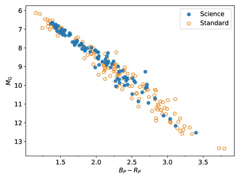
Figure 1: Gaia DR2 $M_{G}$ versus $(B_{p}-R_{p})$ colour magnitude diagram for science targets (filled blue circles) and cool dwarf standards (orange open circles).

2.2 Standard Selection

Given the complexities involved in determining the properties of cool dwarfs, we also observed a set of 136 well characterised late K/M-dwarf standards from the literature. Broadly these standards have parameters from at least one of the following sources:

1. [Fe/H] from an FGK companion,

2. [Fe/H] from low resolution NIR spectra,

3. $T_{\rm eff}$ from interferometry.

With the exception of available interferometric $T_{\rm eff}$ standards, we additionally wanted to source standards from large uniform catalogues due to the known problem of systematics between different spectroscopic techniques (e.g. Lebzelter et al., 2012; Hinkel et al., 2016). With this in mind, the bulk of our M/late-K dwarf standards come from the works of Rojas-Ayala et al. (2012) and Mann et al. (2015), with interferometric targets from von Braun et al. (2012), Boyajian et al. (2012), von Braun et al. (2014), Rabus et al. (2019), and Rains et al. (2020); and FGK companion [Fe/H] compiled by Newton et al. (2014) from Valenti & Fischer (2005), Sousa et al. (2006) and Sozzetti et al. (2009). Our mid-K dwarf calibrators do not come from a single uniform catalogue; they are instead pulled from the works of Woolf & Wallerstein (2005), Sousa et al. (2008), Prugniel et al. (2011), Sousa et al. (2011), Tsantaki et al. (2013), Luck (2017), Luck (2018) and Montes et al. (2018).

These stars were observed with the same instrument settings as our science targets (but at higher SNR), with the intent to provide checks against our analysis techniques for this notoriously complex set of stars.

2.3 Spectroscopic Observations

Observations were conducted using the WiFeS instrument (Wide-Field Spectrograph, Dopita et al., 2007) on the ANU 2.3 m Telescope at Siding Spring Observatory, Australia between August 2019 and September 2020. WiFeS, a dual camera integral field spectrograph, is an effective stellar survey instrument due to its high throughput and broad wavelength coverage. Using the B3000 and R7000 gratings, and RT480 beam splitter, we obtain low resolution blue spectra ($3500\leq\lambda\leq 5700\,$$\text{\,}\mathrm{\SIUnitSymbolAngstrom}$, $\lambda/\Delta\lambda\sim 3000$) and moderate resolution red spectra ($5400\leq\lambda\leq 7000\,$$\text{\,}\mathrm{\SIUnitSymbolAngstrom}$, $\lambda/\Delta\lambda\sim 7000$) with median signal to noise ratios (SNR) per spectral pixel of 16 and 58 respectively. Exposure times ranged from 20 sec to 30 min, and were chosen on the basis of 0.5 magnitude bins in Gaia $G$.

Target observations were bracketed hourly with NeAr Arc lamp exposures, telluric standards were observed every few hours, and flux standards were observed several times throughout each night. Data reduction was done using the standard PyWiFeS pipeline (Childress et al., 2014) with the exception of custom flux calibration due to PyWiFeS’ poor performance with R7000 spectra. Science target observations are listed in Table 7, and standard star observations in Table 9.

Table 1: Science targets

TOIa	TICb	2MASSc	Gaia DR2d	RAd	DECd	$G^{d}$	${B_{p}-R_{p}}^{d}$	Plxd	ruwed	E($B-V$)	N${}_{\rm pc}^{e}$
				(hh mm ss.ss)	(dd mm ss.ss)	(mag)	(mag)	(mas)
741	359271092	09213761-6016551	5299440441521812992	09 21 35.86	-61 43 07.68	8.68	2.03	95.63 $\pm$ 0.03	1.1	0.00	1
731	34068865	09442986-4546351	5412250540681250560	09 44 29.16	-46 13 15.60	9.15	2.32	106.21 $\pm$ 0.03	1.1	0.00	1
260	37749396	00190556-0957530	2428162410789155328	00 19 05.52	-10 02 01.68	9.31	1.70	49.51 $\pm$ 0.06	0.9	0.00	1
836	440887364	15001942-2427147	6230733559097425152	15 00 19.18	-25 32 44.88	9.39	1.55	36.33 $\pm$ 0.04	1.0	0.01	2
562	413248763	09360161-2139371	5664814198431308288	09 36 01.80	-22 20 05.64	9.88	2.40	105.88 $\pm$ 0.06	1.1	0.00	3
455	98796344	03015142-1635356	5153091836072107136	03 01 51.00	-17 24 19.80	10.05	2.59	145.55 $\pm$ 0.08	1.1	0.00	2
139	62483237	22253655-3454346	6598814657249555328	22 25 36.58	-35 05 25.08	10.08	1.45	23.55 $\pm$ 0.04	1.0	0.00	1
253	322063810	00571629-5135048	4928367189956040960	00 57 16.44	-52 24 52.92	10.18	1.71	32.39 $\pm$ 0.03	1.0	0.00	1
134	234994474	23200751-6003545	6491962296196145664	23 20 06.86	-61 56 03.48	10.23	2.03	39.73 $\pm$ 0.04	1.0	0.00	1
544	50618703	05290957-0020331	3220926542276901888	05 29 09.62	-1 39 25.56	10.40	1.57	24.29 $\pm$ 0.04	1.1	0.01	1
486	260708537	06334998-5831426	5482827676662168832	06 33 49.18	-59 28 30.00	10.53	2.43	65.70 $\pm$ 0.03	1.2	0.00	1
177	262530407	01214538-4642518	4933912198893332224	01 21 45.22	-47 17 07.08	10.55	2.17	44.46 $\pm$ 0.05	1.0	0.00	1
129	201248411	00004490-5449498	4923860051276772608	00 00 44.54	-55 10 09.12	10.59	1.39	16.16 $\pm$ 0.02	1.1	0.00	1
175	307210830	08180763-6818468	5271055243163629056	08 18 07.90	-69 41 07.80	10.60	2.51	94.14 $\pm$ 0.03	1.1	0.00	3
824	193641523	14483982-5735175	5880886001621564928	14 48 39.72	-58 24 39.96	10.72	1.36	15.61 $\pm$ 0.03	1.1	0.02	1
133	219338557	23373497-5857166	6489346046933733632	23 37 35.38	-59 02 41.64	10.72	1.53	20.53 $\pm$ 0.03	1.0	0.00	1
1130	254113311	19053021-4126151	6715688452614516736	19 05 30.24	-42 33 44.64	10.88	1.55	17.14 $\pm$ 0.05	1.1	0.01	2
198	12421862	00090428-2707196	2333676738049780352	00 09 05.16	-28 52 41.88	10.92	1.99	42.12 $\pm$ 0.05	1.0	0.00	1
833	362249359	09423526-6228346	5250780970316845696	09 42 34.92	-63 31 26.76	11.05	1.83	23.94 $\pm$ 0.02	0.8	0.01	1
178	251848941	00291228-3027133	2318295979126499200	00 29 12.48	-31 32 45.24	11.15	1.49	15.92 $\pm$ 0.05	1.2	0.00	3
279	122613513	02444524-3212391	5063070558501465856	02 44 45.24	-33 47 20.40	11.20	1.44	13.42 $\pm$ 0.04	1.1	0.00	1
704	260004324	06042035-5518468	5500061456275483776	06 04 21.60	-56 41 18.60	11.23	2.22	33.48 $\pm$ 0.03	1.0	0.00	1
1078	370133522	20274210-5627262	6468968316900356736	20 27 42.86	-57 32 15.72	11.24	2.32	49.06 $\pm$ 0.05	1.0	0.00	1
969	280437559	07403284+0205561	3087206553745290624	07 40 32.81	+2 05 54.96	11.25	1.47	12.92 $\pm$ 0.05	1.4	0.01	1
620	296739893	09284158-1209551	5738284016370287616	09 28 41.62	-13 49 58.08	11.31	2.24	30.25 $\pm$ 0.05	1.0	0.00	1
910	369327947	19205439-8233170	6347643496607835520	19 20 57.10	-83 26 24.72	11.42	2.73	80.09 $\pm$ 0.04	1.1	0.00	1
713	167600516	06480517-6537252	5285060409961261696	06 48 05.14	-66 22 32.52	11.42	1.52	14.39 $\pm$ 0.02	0.9	0.01	2
932	260417932	06234590-5434414	5499671713762981248	06 23 45.82	-55 25 19.20	11.42	1.41	11.68 $\pm$ 0.02	0.8	0.01	2
240	101948569	00590112-4409389	4982951791883929472	00 59 01.18	-45 50 20.76	11.43	1.50	13.33 $\pm$ 0.03	1.1	0.00	1
696	77156829	04324261-3947112	4864160624337973248	04 32 42.96	-40 12 32.76	11.54	2.28	50.28 $\pm$ 0.02	1.1	0.00	2
244	118327550	00421695-3643053	5001098681543159040	00 42 16.75	-37 16 55.20	11.55	2.55	45.36 $\pm$ 0.07	1.3	0.00	1
270	259377017	04333970-5157222	4781196115469953024	04 33 39.86	-52 02 33.36	11.63	2.33	44.46 $\pm$ 0.03	1.0	0.00	3
912	406941612	15172165-8028225	5772442647192375808	15 17 18.86	-81 31 36.12	11.64	2.40	38.27 $\pm$ 0.02	1.1	0.01	1
475	100608026	05465951-3231592	2901089987127041920	05 46 59.59	-33 28 03.00	11.70	1.76	16.99 $\pm$ 0.02	1.0	0.01	1
442	70899085	04164560-1205023	3189306030970782208	04 16 45.65	-13 54 54.36	11.73	1.99	18.98 $\pm$ 0.04	1.2	0.00	1
761	165317334	11570326-3806169	3460168250866990848	11 57 03.12	-39 53 42.72	11.73	1.73	14.94 $\pm$ 0.04	1.2	0.01	1
870	219229644	04131645-5056400	4782093729275660160	04 13 16.63	-51 03 20.52	11.78	1.99	18.56 $\pm$ 0.02	1.1	0.00	1
904	261257684	05572938-8307486	4620844400530949376	05 57 29.11	-84 52 13.08	11.84	2.02	21.67 $\pm$ 0.02	1.0	0.01	1
732	36724087	10183516-1142599	3767281845873242112	10 18 34.78	-12 16 55.92	11.85	2.69	45.46 $\pm$ 0.08	1.1	0.00	2
656	36734222	10193800-0948225	3767805209112436736	10 19 37.97	-10 11 36.96	11.89	1.63	11.50 $\pm$ 0.04	1.1	0.01	1
1075	351601843	20395334-6526579	6426188308031756288	20 39 53.09	-66 33 01.08	12.05	1.84	16.24 $\pm$ 0.02	1.2	0.00	1
700	150428135	06282325-6534456	5284517766615492736	06 28 22.97	-66 25 17.04	12.06	2.39	32.10 $\pm$ 0.02	1.1	0.00	3
727	149788158	08425684-0229529	3072157538091829120	08 42 56.86	-3 30 05.04	12.07	2.15	23.24 $\pm$ 0.03	1.1	0.00	1
249	179985715	00561930-3856552	4987729474846997248	00 56 19.20	-39 03 02.88	12.08	1.70	14.13 $\pm$ 0.03	1.1	0.00	1
1201	29960110	02485926-1432152	5157183324996790272	02 48 59.45	-15 27 45.72	12.10	2.37	26.37 $\pm$ 0.04	1.1	0.00	1

Notes: ^a TESS Object of Interest ID, ^b TESS Input Catalogue ID (Stassun et al., 2018, 2019),^c2MASS (Skrutskie et al., 2006), ^cGaia (Brown et al., 2018) - note that Gaia parallaxes listed here have been corrected for the zeropoint offset, ^dNumber of candidate planets, NASA Exoplanet Follow-up Observing Program for TESS

Table 2: continued

Science targets TOI^a TIC^b 2MASS^c Gaia DR2^d RA^d DEC^d $G^{d}$ ${B_{p}-R_{p}}^{d}$ Plx^d ruwe^d E($B-V$) N${}_{\rm pc}^{e}$ (hh mm ss.ss) (dd mm ss.ss) (mag) (mag) (mas) 875 14165625 05120890-3742313 4820828591913853696 05 12 08.93 -38 17 29.40 12.12 1.51 9.39 $\pm$ 0.02 1.0 0.01 1 929 175532955 03033741-3955515 5044287532642519680 03 03 37.73 -40 04 09.12 12.13 1.42 8.71 $\pm$ 0.02 1.1 0.01 1 493 19025965 07583071+1253005 3151371883379694720 07 58 30.65 +12 52 59.88 12.19 1.56 9.29 $\pm$ 0.04 1.1 0.01 1 1216 141527965 05505139-7541200 4648441970589471104 05 50 51.55 -76 18 41.04 12.31 1.62 10.02 $\pm$ 0.03 1.2 0.01 1 233 415969908 22545039-1854426 2402715141877299584 22 54 50.06 -19 05 15.36 12.41 2.27 29.58 $\pm$ 0.04 1.0 0.00 2 711 38510224 04100386-6156326 4676789514954240768 04 10 03.86 -62 03 26.28 12.45 1.45 8.43 $\pm$ 0.02 1.0 0.01 1 876 32497972 05362611-2414377 2963392606627366912 05 36 26.23 -25 45 20.16 12.47 1.87 12.76 $\pm$ 0.03 1.1 0.01 1 785 374829238 05532099-6538022 4755884700667639296 05 53 20.95 -66 21 59.40 12.51 2.04 15.23 $\pm$ 0.02 1.0 0.01 1 406 153065527 03170297-4214323 4851053999056603904 03 17 03.02 -43 45 21.24 12.55 2.71 32.17 $\pm$ 0.04 1.2 0.00 2 714 219195044 06093401-5349245 5500474185452572032 06 09 34.18 -54 10 37.20 12.56 2.04 18.54 $\pm$ 0.02 1.2 0.01 2 900 210873792 16233735-3122228 6037266684232926208 16 23 37.22 -32 37 35.04 12.59 1.52 8.23 $\pm$ 0.05 0.9 0.03 1 557 55488511 03560411-1016192 3193508849745633280 03 56 04.27 -11 43 40.80 12.60 1.92 13.14 $\pm$ 0.04 1.1 0.01 1 864 231728511 05254662-5121253 4772266186971169792 05 25 46.42 -52 38 34.80 12.66 2.42 26.22 $\pm$ 0.03 1.1 0.01 1 256 92226327 00445930-1516166 2371032916186181760 00 44 59.66 -16 43 33.24 12.67 3.04 66.70 $\pm$ 0.07 1.1 0.00 2 702 237914496 03444203-6511567 4672700190692201088 03 44 41.98 -66 48 06.12 12.68 1.80 11.82 $\pm$ 0.03 1.1 0.01 1 1082 261108236 05330624-8048563 4621526273835900288 05 33 06.19 -81 11 04.20 12.68 1.70 9.95 $\pm$ 0.03 1.1 0.01 1 672 151825527 11115769-3919400 5396580575830873728 11 11 57.82 -40 40 18.84 12.72 2.13 14.92 $\pm$ 0.03 1.1 0.01 1 806 33831980 04134003-7605515 4627952094666051072 04 13 39.86 -77 54 07.20 12.77 1.67 9.55 $\pm$ 0.02 1.3 0.01 1 797 271596225 07141480-7436089 5262540590756812032 07 14 15.14 -75 23 48.84 12.78 2.20 17.77 $\pm$ 0.02 1.1 0.01 2 663 54962195 10401596-0830385 3762515188088861184 10 40 15.82 -9 29 20.04 12.81 2.13 15.54 $\pm$ 0.04 1.0 0.01 2 540 200322593 05051443-4756154 4785886941312921344 05 05 14.33 -48 03 45.00 12.89 3.11 71.39 $\pm$ 0.04 1.0 0.00 1 285 220459976 04584731-5623385 4764216563561182336 04 58 47.33 -57 36 22.32 13.07 1.79 8.61 $\pm$ 0.02 0.9 0.01 1 674 158588995 10582099-3651292 5400949450924312576 10 58 20.78 -37 08 30.84 13.08 2.53 21.67 $\pm$ 0.05 1.5 0.01 1 789 300710077 07410444-7118157 5264306681309492864 07 41 04.85 -72 41 46.32 13.15 2.44 23.01 $\pm$ 0.03 1.3 0.01 1 873 237920046 03465622-6320142 4673392195823039744 03 46 56.78 -64 39 47.16 13.16 2.09 12.97 $\pm$ 0.02 1.3 0.01 1 698 141527579 05505661-7637132 4647922867959139072 05 50 57.38 -77 22 49.44 13.26 2.33 15.75 $\pm$ 0.03 1.2 0.01 1 136 410153553 22415815-6910089 6385548541499112448 22 41 59.09 -70 49 40.44 13.39 3.40 67.15 $\pm$ 0.05 1.1 0.00 1 269 220479565 05032306-5410378 4770828304936109056 05 03 23.11 -55 49 20.28 13.41 2.30 17.51 $\pm$ 0.02 1.1 0.01 1 654 35009898 10585379-0532468 3788670679927991296 10 58 53.90 -6 27 09.00 13.42 2.51 17.29 $\pm$ 0.05 1.1 0.01 1 782 429358906 12154108-1854365 3518374197418907648 12 15 40.90 -19 05 22.92 13.55 2.71 19.01 $\pm$ 0.07 1.2 0.01 1 521 27649847 08132251+1213181 649852779797683968 08 13 22.63 +12 13 19.56 13.58 2.44 16.38 $\pm$ 0.06 1.3 0.00 1 203 259962054 02520450-6741155 4647534190597951232 02 52 04.34 -68 18 46.80 13.59 2.94 40.31 $\pm$ 0.05 1.4 0.00 1 532 144700903 05401918+1133463 3340265717587057536 05 40 19.22 +11 33 45.36 13.63 1.93 7.38 $\pm$ 0.03 1.1 0.02 1 756 73649615 12482523-4528140 6129327525817451648 12 48 24.89 -46 31 46.20 13.66 2.31 11.58 $\pm$ 0.04 1.2 0.02 1 302 229111835 01095538-5214219 4927215760764862976 01 09 55.51 -53 45 37.80 13.71 1.64 5.10 $\pm$ 0.01 1.0 0.01 1 435 44647437 03573850-2511238 5082797618168232320 03 57 38.54 -26 48 36.36 13.75 1.73 6.02 $\pm$ 0.02 1.1 0.01 1 1067 201642601 19144126-5934458 6638412919991750912 19 14 41.28 -60 25 14.16 13.82 1.43 3.76 $\pm$ 0.02 1.0 0.03 1 210 141608198 05555049-7359046 4650160717726370816 05 55 50.83 -74 00 52.92 13.84 2.83 23.33 $\pm$ 0.05 1.3 0.01 1 1073 158297421 19095625-4939538 6658373007402886400 19 09 56.26 -50 20 06.36 14.31 1.43 3.30 $\pm$ 0.04 1.0 0.04 1 468 33521996 05523523-1901539 2966680597368750720 05 52 35.23 -20 58 06.24 14.34 2.01 5.88 $\pm$ 0.04 1.2 0.01 1 122 231702397 22114728-5856422 6411096106487783296 22 11 47.57 -59 03 14.04 14.34 2.64 16.07 $\pm$ 0.06 1.2 0.00 1 507 348538431 08063103-1545526 5724250571514167424 08 06 31.10 -16 14 07.08 14.48 2.69 8.99 $\pm$ 0.06 1.3 0.01 1 551 192826603 05305145-3637508 4821739369794767744 05 30 51.41 -37 22 08.40 14.83 1.84 4.56 $\pm$ 0.02 1.0 0.02 1 552 44737596 04034783-2524320 5082914338199586560 04 03 47.86 -26 35 27.96 14.87 2.15 5.10 $\pm$ 0.03 1.1 0.01 1 234 12423815 00101648-2616566 2335244779070099200 00 10 16.54 -27 43 03.36 15.69 2.17 3.98 $\pm$ 0.07 1.1 0.01 1 555 170849515 04412154-3219128 4877426575724467456 04 41 21.55 -33 40 46.56 15.71 1.80 2.56 $\pm$ 0.04 1.0 0.04 1 142 425934411 00182539-6250523 4901321849613348736 00 18 25.42 -63 09 07.56 15.77 2.16 3.09 $\pm$ 0.04 1.0 0.01 1

2.4 Radial velocity determination

Radial velocities of the WiFeS R7000 spectra were determined from a least squares minimisation of a set of synthetic template spectra varying in temperature (see Section 4.1 for details of model grid). We use a coarsely sampled version of this grid, computed at R$\sim 7000$ over $5400\leq\lambda\leq 7000$ for $3000\leq T_{\rm eff}\leq 5500\,$K, $\log g=4.5$, and [Fe/H]$=0.0$, with $T_{\rm eff}$ steps of $100\,$K for radial velocity determination. For further information on our RV fitting formalism, see Žerjal et al. (2021).

Statistical uncertainties on this approach are median $\sim$410 m s^-1, though comparison to Gaia DR2 in Figure 2 reveals a larger scatter with standard deviation $\sim$$4.5\,$km s^-1, computed from a median absolute deviation, which we add in quadrature with our statistical uncertainties. Higher uncertainties are consistent with the work of Kuruwita et al. (2018) who found that WiFeS varies on shorter timescales than our hourly arcs can account for. While they additionally improved precision by calibrating using oxygen B-band absorption, RV uncertainties of $\sim$$4.5\,$km s^-1 are sufficient for this work. Our final values are reported in Table 7 for science targets, and Table 9 for standards.

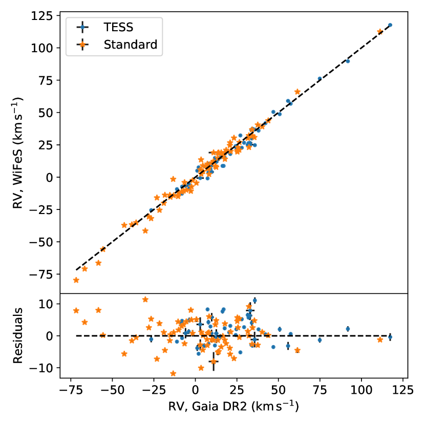
Figure 2: Comparison between those stars with radial velocities in Gaia DR2 and our work here, from which we determine a scatter of $\sim$$4.5\,$km s^-1.

3 Photometric Metallicity Calibration

As established earlier, cool dwarf metallicities are notoriously difficult to determine, particularly when working with optical spectra. Bonfils et al. (2005) initially proposed empirical calibrations to determine [Fe/H] from a star’s position in $M_{K}-(V-K)$ space, a technique which was later iterated on by Johnson & Apps (2009), Schlaufman & Laughlin (2010), and Neves et al. (2012). Such relations are based on the fact that once on the main sequence, low mass stars do not evolve (and hence change in brightness and temperature) appreciably on moderate timescales as compared to their higher mass and faster evolving counterparts. Thus, assuming no extra scatter from unresolved binaries and standard helium enrichment (e.g. Pagel & Portinari, 1998), a star’s position above or below the mean main sequence is directly correlated with its chemical composition (Baraffe et al., 1998).

These relations are benchmarked on what is considered the gold standard for M-dwarf metallicites: [Fe/H] from a hotter FGK companion taken to have formed at the same time and thus have the same chemical composition. This chemical homogeneity is now well established for FGK-FGK pairs (e.g. Desidera et al., 2004; Hawkins et al., 2020). The process of determining which stars on the sky are likely associated has now been greatly simplified with the release of Gaia DR2, which has provided precision parallax measurements and proper motions for nearly all nearby M-dwarfs, with our sample of secondaries having median $0.17\,$% parallax precision.

We take as input the sample of FGK-KM-dwarf pairs compiled by Mann et al. (2013a) and Newton et al. (2014). These combine primary star [Fe/H] measurements from high resolution spectra sourced from a variety of previous surveys (Mishenina et al., 2004; Luck & Heiter, 2005; Valenti & Fischer, 2005; Bean et al., 2006a; Ramírez et al., 2007; Robinson et al., 2007; Fuhrmann, 2008; Casagrande et al., 2011; da Silva et al., 2011; Mann et al., 2013a), with Mann et al. (2013a) correcting for inter-survey systematics to place them on a common [Fe/H] scale. To this set we add the metal-poor, cool subdwarf VB12 to extend our metallicity coverage, taking the [Fe/H] reported by Ramírez et al. (2007) for its primary HD 219617 AB (and correcting for the systematic reported by Mann et al. 2013a). This provided 128 total pairs, which was reduced to 69 after crossmatching with both Gaia DR2 and 2MASS, and removing those stars with missing or poor photometry (2MASS Qflg$\neq$‘AAA’, where ‘AAA’ is the highest photometric quality rating and corresponds to $JHK_{S}$ respectively); those flagged on SIMBAD as spectroscopic binaries; those with poor Gaia astrometry (Gaia dup flag=1, RUWE $>1.4$); those pairs with M dwarf primaries; or whose parallaxes, astrometry, and RVs indicate they aren’t associated with the putative primary. These 69 stars are listed in Table 15, and span $-1.28<{\rm[Fe/H]}<+0.56$.

From this sample we follow the approaches of Johnson & Apps (2009) and Schlaufman & Laughlin (2010) and use a polynomial to trace the mean main sequence in $M_{K_{S}}-$colour space, though using $(B_{P}-K_{S})$ instead of $(V-K_{S})$. For our main sequence fit, we use the complete Mann et al. (2015) sample of cool dwarfs with Gaia parallaxes, which spans a wider range in $(B_{P}-K_{S})$ and is less sparse than the assembled sample of M-dwarf secondaries. We find the following third order polynomial sufficient to describe the main sequence:

$$(B_{P}-K_{S})=a_{3}M_{K_{S}}^{3}+a_{2}M_{K_{S}}^{2}+a_{1}M_{K_{S}}+a_{0}$$ (1)

where $a_{3}=0.05385$, $a_{2}=-1.08356$, $a_{1}=7.76175$, and $a_{0}=-14.54705$. We then calculate the offset in $(B_{P}-K_{S})$ from this polynomial (as a colour offers greater discriminatory power than $M_{K_{S}}$, Schlaufman & Laughlin 2010), and use least squares to find the best fitting linear relation for [Fe/H]:

$${\rm[Fe/H]}=b_{1}\Delta(B_{P}-K_{S})+b_{0}$$ (2)

where $b_{1}$ and $b_{0}$ are the linear polynomial coefficients. After correcting for a remaining trend in the residuals, our adopted coefficients are $b_{1}=0.71339$, and $b_{0}=-0.04301$. This relation is valid for stars with $1.51<(B_{P}-R_{P})<3.3$ (based on the hottest and coolest secondaries respectively), and has an uncertainty of $\pm 0.19\,$dex (from the standard deviation in the residuals). We stress that the relation should only be used for stars that pass the same quality cuts we use to build the relation: unsaturated photometry, not flagged as a duplicate source in Gaia, RUWE $<1.4$, and not a known/suspected spectroscopic binary or pre-main sequence star. Our [Fe/H] recovery and fits can be seen in Figure 3.

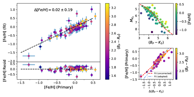
Figure 3: Left: Cool dwarf secondary [Fe/H] calculated from our photometric calibration vs [Fe/H] from the associated FGK primary star, colour coded by Gaia $(B_{P}-R_{P})$. The standard deviation of the residuals, and our adopted uncertainty for the relation, is $\pm 0.19\,$dex. See Table 15 for further information on this FGK-KM binary calibration sample. Top Right: $M_{K_{S}}-(B_{P}-K_{S})$ colour magnitude diagram for the calibration sample of cool dwarf secondaries colour coded by host star [Fe/H]. The dashed red line is a third order polynomial representing the main sequence, fitted to the Mann et al. (2015) sample of cool dwarfs. Bottom Right: Fitted [Fe/H] as a function $\Delta(B_{P}-K_{S})$ offset from the mean main sequence polynomial. The dashed red line is the initial uncorrected linear least squares fit, and the dash-dotted blue line is the adopted fit after correcting for the remaining trend in the residuals

4 Spectroscopic Analysis

The TESS candidate planet host observing program described here developed from an ANU 2.3 m/WiFeS survey of potential young stars (Žerjal et al., 2021) to identify signs of youth (via Balmer Series and Ca II H&K emission, and Li 6708$\text{\,}\mathrm{\SIUnitSymbolAngstrom}$ absorption) and determine RVs to enable kinematic analysis with Chronostar (Crundall et al., 2019) when combined with Gaia astrometry. While their spectral type coverage ($1.27<B_{P}<2.6$) was relatively similar to our own, instrument setup however prioritised higher spectral resolution for improved velocity precision and coverage of the key wavelength regions of interest. These regions are firmly in the optical, where M-dwarf spectral features are strongly blended and heavily dominated by molecular absorption from hydrides (e.g. MgH, CaH, SiH) and oxides (e.g. TiO, VO, ZrO). This is in contrast to most of the previous low-medium resolution studies of M-dwarfs which work in the NIR where the absorption is less severe and many more [Fe/H] sensitive features are available.

Here we describe our attempts to derive reliable atmospheric parameters from our spectra using a model based approach. Our investigation ultimately revealed substantial systematics and degeneracies when fitting to model optical spectra, resulting in our inability to recover $\log g$ or [Fe/H]. While the spectra are included in our temperature fitting routine, they are primarily used for RV determination, identification of peculiarities (such as signs of youth), and for testing model fluxes. The details of our findings are covered below, and we await follow-up work to explore a standard-based or data-driven approach (e.g. similar to the work of Birky et al. 2020, but in the optical) to take full advantage of the information in our now large library of optical cool dwarf spectra.

4.1 Selection of Model Atmosphere Grid

While synthetic spectra show better agreement for FGK stars, the onset of strong molecular features such as TiO and H₂O in the atmospheres of late K and M dwarf atmospheres make the task of modelling their spectra far more complex. There are known historical issues, for instance, when computing optical colours from synthetic spectra (e.g. difficulties in computing accurate $V$ band magnitudes, Leggett et al. 1996), and the line lists required are considerably more complicated. Thus, before using models in our automatic fitting routine, we first investigate their performance at different wavelengths to flag regions requiring special consideration. For the purposes of this comparison, we check the MARCS grid of stellar atmospheres against the BT-Settl grid (Allard et al., 2011), both of which are described in detail below.

Our template grid of 1D LTE MARCS spectra was previously described by Nordlander et al. (2019) and computed using the TURBOSPECTRUM code (v15.1; Alvarez & Plez 1998; Plez 2012) and MARCS model atmospheres (Gustafsson et al., 2008). The spectra are computed with a sampling resolution of $1\,$km s^-1, corresponding to a resolving power of $R\sim 300\,000$, with a microturbulent velocity of $1\,$km s^-1. We adopt the solar chemical composition and isotopic ratios from Asplund et al. (2009), except for an alpha enhancement that varies linearly from $\text{[}\alpha/\text{Fe}]=0$ when $\rm[Fe/H]\geq 0$ to $\text{[}\alpha/\text{Fe}]=+0.4$ when $\rm[Fe/H]\leq-1$. We use a selection of atomic lines from VALD3 (Ryabchikova et al., 2015) together with roughly 15 million molecular lines representing 18 different molecules, the most important of which for this work are CaH (Plez, priv. comm.), MgH (Kurucz, 1995; Skory et al., 2003), and TiO (Plez, 1998, with updates via VALD3).

MARCS model fluxes were developed for usage over a range of spectral types including both cool giants and, critically for our work here, cool dwarfs. Recent work fitting cool dwarf stellar atmospheres however have mostly used high-resolution NIR spectra (J band: Önehag et al. 2012; Lindgren et al. 2016; Lindgren & Heiter 2017; H band: Souto et al. 2017, 2018) rather than the medium resolution optical spectra we use here.

For BT-Settl, we use the most recently published grid (Allard et al., 2012a, b; Baraffe et al., 2015) which uses abundances from Caffau et al. (2011) and covers $1200<T_{\rm eff}<7000\,$K, $2.5<\log g<5.5$, [M/H]$=0.0$. Note that while older grids have a wider range of [M/H], they are also less complete in terms of physics and line lists, so we opt for the newest grid for our comparison here, and limit ourselves to testing on stars with approximately Solar [Fe/H].

BT-Settl atmospheres have been developed with a focus on cool dwarf atmospheres and have a strong history of use for studying cool dwarfs at a variety of wavelengths and resolutions (e.g. Rojas-Ayala et al., 2012; Muirhead et al., 2012; Mann et al., 2012; Rajpurohit et al., 2013; Lépine et al., 2013; Gaidos et al., 2014; Mann et al., 2013c; Mann et al., 2015; Veyette et al., 2016; Veyette et al., 2017; Souto et al., 2018). Most noteworthy for our comparison are tests by Reylé et al. (2011) and Mann et al. (2013c), which examined model performance at optical wavelength regions $>5500\,$$\text{\,}\mathrm{\SIUnitSymbolAngstrom}$ common to our WiFeS R7000 spectra.

For each of our standard stars we combined and normalised our flux calibrated B3000 and R7000 spectra to give a single spectrum with $3500<\lambda<7000\,$$\text{\,}\mathrm{\SIUnitSymbolAngstrom}$. To this we compared synthetic MARCS fluxes interpolated to literature values of $T_{\rm eff}$, $\log g$, and [Fe/H], as well as the BT-Settl equivalent for those with close to Solar [Fe/H]. Given our large library of standards we were able to observe model performance as a function of both stellar parameters and wavelength. A representative comparison (with overplotted filter bandpasses) is shown in Figure 4, and our main conclusions are summarised as follows:

• Both MARCS and BT-Settl models severely overpredict (worsening with decreasing $T_{\rm eff}$) flux blueward of $\sim$5400 $\text{\,}\mathrm{\SIUnitSymbolAngstrom}$. The MARCS systematic offset is also a strong function of [Fe/H], an effect also observed in Joyce & Chaboyer (2015), and while this is likely also true for BT-Settl, we cannot comment definitively while limited to the Solar [Fe/H] grid.

• BT-Settl additionally underpredicts flux at $\sim$6500 $\text{\,}\mathrm{\SIUnitSymbolAngstrom}$ (as expected from Reylé et al. 2011 and Mann et al. 2013c).

• Synthetic photometry generated in SkyMapper $v$, $g$, $r$, and Gaia $B_{P}$ is thus systematically brighter than the observed equivalents for reasonable assumptions of $T_{\rm eff}$, $\log g$, and [Fe/H] for the star under consideration.

We are able to quantify these systematics by integrating photometry from our flux calibrated observed spectra and comparing to the MARCS synthetic equivalents generated at the literature parameters for each star. Our wavelength coverage allows us to check the magnitude offsets $\Delta v$, $\Delta g$, $\Delta r$ and $\Delta B_{P}$, corresponding to $v$, $g$, $r$, and $B_{P}$ respectively. We note that for the purpose of this comparison we do not account for inaccuracies in our flux calibration, telluric absorption, nor for WiFeS not covering the bluest $\sim 200\,$$\text{\,}\mathrm{\SIUnitSymbolAngstrom}$ of $B_{P}$. However, checks with synthetic spectra show that this region accounts for less than $0.25\,$% of $B_{P}$ flux at 3000 K where our correction is greatest, and remains less than $0.5\,$% of flux at 4,500 K where our correction is more modest. These offsets are shown for $g$, $r$, and $B_{P}$ in Figure 5, and fit separately for each filter by the following linear relation in observed Gaia DR2 $(B_{P}-R_{P})$:

$$\Delta m_{\zeta}=a_{1}(B_{P}-R_{P})+a_{0}$$ (3)

where $\Delta m_{\zeta}$ is the magnitude offset in filter $\zeta$; $a_{1}$ equals 0.116, 0.084, and 0.034 for $g$, $r$, and $B_{P}$ fits respectively; and $a_{0}$ equals -0.072, -0.069, and -0.037 for $g$, $r$, and $B_{P}$ fits respectively. Computing the standard deviation for the residuals shows 0.10, 0.05, and 0.02 uncertainties in magnitude (equivalent to roughly 10%, 5%, and 2% uncertainties in flux) for $g$, $r$, and $B_{P}$ respectively. From this we conclude that while the corrections to $r$, and $B_{P}$ are modest, $g$ is likely too affected to prove useful.

Following this both qualitative and quantitative investigation comparing model fluxes to our library of standard star spectra, we make the following decisions for our synthetic fitting methodology:

• Given similar observed systematics for both MARCS and BT-Settl model fluxes, we adopt the MARCS grid to enable fitting for [Fe/H] as well as $T_{\rm eff}$ and $\log g$.

• Only use our R7000 spectra ($5400\leq\lambda\leq 7000\,$$\text{\,}\mathrm{\SIUnitSymbolAngstrom}$) for fitting, additionally masking out the two regions worst affected by missing opacities (5498-5585 $\text{\,}\mathrm{\SIUnitSymbolAngstrom}$ and 6029-6159 $\text{\,}\mathrm{\SIUnitSymbolAngstrom}$).

• Apply an observed $(B_{P}-R_{P})$ dependent systematic offset to our generated synthetic $B_{P}$ and $r$ photometry per Equation 3.

• Given the widespread historical use and success of studying M-dwarfs at NIR wavelengths, we use $R_{P}$, $i$, $z$, $J$, $H$, and $K_{S}$ photometry assuming no substantial model systematics.

• However, to account for remaining model uncertainties, we add conservative $\pm 0.011$ magnitude (1% in flux) uncertainties in quadrature with the observed uncertainties for $R_{P}$, $i$, $z$; and the fitted $\pm 0.02$ for $r$, and $\pm 0.05$ for $B_{P}$.

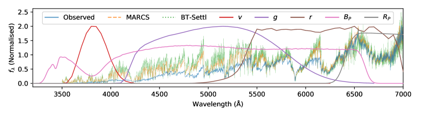
Figure 4: Observed WiFeS B3000 and R7000 spectra for GJ 447, along with a MARCS synthetic spectrum interpolated to the parameters from Mann et al. 2015 ($T_{\rm eff}=3192\,$K, $\log g=5.04$, [Fe/H] $=-0.02$), and a PHOENIX/BT-Settl spectrum at the closest grid point available ($T_{\rm eff}=3200\,$K, $\log g=5.0$, [Fe/H] $=0.0$). SkyMapper $v$, $g$, $r$, and Gaia $B_{P}$ and $R_{P}$ filters are overplotted for reference. Note the severe model disagreement below 5400 $\text{\,}\mathrm{\SIUnitSymbolAngstrom}$.

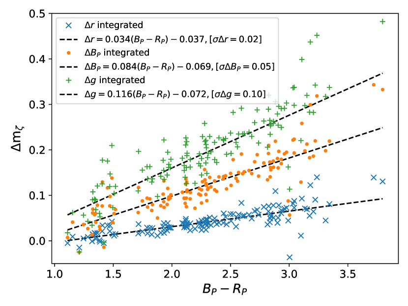
Figure 5: Gaia $B_{P}$, and SkyMapper $gr$ systematic offsets between integrated flux calibrated WiFeS spectra and MARCS model integrated spectra at literature parameters for our standard stars, plotted as a function of observed Gaia $B_{P}-R_{P}$. Stars redder in $B_{P}-R_{P}$ have systematically more flux at bluer wavelengths, with the best fit linear magnitude offset plotted for each filter, and the standard deviation in magnitude noted.

4.2 Synthetic Fitting

Our approach to spectral fitting was developed specifically to work with the complicated spectra of our cool star sample and incorporates nine distinct sources of information. While it was hoped that this methodology would be sufficient to disentangle the strong degeneracy between $T_{\rm eff}$ and [Fe/H] and accurately recover distant-independent [Fe/H] for our standard sample, this ultimately proved not to be the case. While we are able to tightly constrain $T_{\rm eff}$, we must resort to using the photometric [Fe/H] relation developed in Section 3 to fix [Fe/H] during the fit. The information included in our fit is as follows:

1. Medium resolution R7000 optical spectra from WiFeS,

2. Observed Gaia $B_{P}$, $R_{P}$; 2MASS $J$, $H$, and $K_{S}$; and SkyMapper DR3 $r$, $i$, $z$ photometry,

3. Empirical cool dwarf radius relations from Mann et al. (2015) - valid for K7-M7 stars, and used to estimate $\log g$,

4. Empirical cool dwarf mass relations from Mann et al. (2019) - valid for $0.075M_{\odot}<M_{\star}<0.70M_{\odot}$, and used to estimate $\log g$,

5. Synthetic MARCS model spectra (for spectral fitting, interpolated to the resolution and wavelength grid of WiFeS)

6. MARCS model fluxes (for photometric fitting),

7. Stellar parallaxes from Gaia DR2,

8. The interstellar dust map from Leike & Enßlin (2019),

9. A set of reference stellar standards with known parameters for testing and validation purposes (see Section B for details).

We found that least squares fitting between real and synthetic spectra alone consistently underestimated expected $\log g$ values of our sample by up to $0.3\,$dex - physical for a set of young stars, but not realistic for our overwhelmingly main sequence sample. To counter this, we calculate $\log g$ using the absolute $K_{S}$ band radius and mass relations of Mann et al. (2015) and Mann et al. (2019) respectively, and fix it during fitting. We then use a two step iterative procedure, with the first fit fixing $\log g$ to the value from empirical relations, and a second and final fit using our interim measured radius and a mass from Mann et al. (2019). All of our TESS targets fall within the stated $4<M_{K_{S}}<11$ limits for the mass relation. Although the relation is only valid for main sequence stars, we employ it with caution for two suspected young stars TOI 507 (TIC 348538431) and TOI 142 (425934411), both discussed in more detail in Section 6.5, on the assumption that the resulting value of $\log g$ will still be more accurate than an unconstrained synthetic fit. Additionally, we suspect TOI 507 of being a near-equal mass binary, and as such treat it as $0.75$ magnitudes fainter (or half as bright) for the purpose of using the relation, equivalent to determining the mass for only a single component.

While this now solves the $\log g$ issue, we are still left with two issues arising from the spectra themselves. The first is that certain wavelength regions of our MARCS model spectra are a poor match compared to our reference sample with known $T_{\rm eff}$, $\log g$, and [Fe/H] - particularly at cooler temperatures. As discussed in Section 4.1, we account for this by using only spectra from the red arm of WiFeS with $\lambda>5400\,$A, and masking out remaining regions with poor agreement.

The second remaining issue is that of the degeneracy between $T_{\rm eff}$ and [Fe/H] when fitting spectra. This effect is caused by both the temperature and metallicity influencing the strength of atmospheric molecular absorbers or opacity sources (predominantly TiO in the optical, but also various hydrides). What this means in practice is that there often isn’t a single minimum or optimal set of atmospheric parameters when fitting synthetic spectra, but instead there exists a range of good fits (or even multiple minima) at different combinations of $T_{\rm eff}$ and [Fe/H] - possibly separated by several 100 K in $T_{\rm eff}$ or several 0.1 dex in [Fe/H].

In an attempt to overcome this, we include photometry from redder wavelengths that are less dominated by absorption than optical wavelengths, meaning that $T_{\rm eff}$ and [Fe/H] are less degenerate. While we do not have NIR spectra for our science or reference sample, we do have Gaia, SkyMapper, and 2MASS photometry in the form of $B_{P}$, $R_{P}$, $r$, $i$, $z$, $J$, $H$, and $K_{S}$ which together give us almost continuous wavelength coverage out to nearly 2.4$\,\mu$m and covers the bulk of stellar emission for our cool stars.

We thus modified our fitting methodology to also compute the uncertainty weighted residuals between observed and synthetic stellar photometry. In order to compare synthetic photometry to its observed equivalent we formulate the fit as follows:

$$m_{\zeta,m}={\rm BC}_{\zeta}(T_{\rm eff},\log g,{\rm[Fe/H]})+m_{\rm bol}$$ (4)

where $m_{\zeta,m}$ is the model magnitude in filter $\zeta$; ${\rm BC}_{\zeta}$ is the bolometric correction (i.e. the total flux outside of a filter $\zeta$) as a function of $T_{\rm eff}$, $\log g$, and [Fe/H] in filter $\zeta$; and $m_{\rm bol}$ is the apparent bolometric magnitude (i.e. the apparent magnitude of the star over all wavelengths). In this implementation $m_{\rm bol}$ serves as a physically meaningful free parameter used to scale synthetic magnitudes to their observed equivalents and ultimately allow computation of the apparent bolometric flux $f_{\rm bol}$. This is done using the well tested bolometric-corrections software (Casagrande & VandenBerg, 2014, 2018a, 2018b) to interpolate a grid of bolometric corrections from MARCS fluxes in different filters for the stellar parameters at each fitting call. By fitting for $m_{\rm bol}$ and using bolometric corrections, we are thus directly able to compare an observed magnitude, $m_{\zeta,o}$, from Gaia, SkyMapper, or 2MASS directly with its MARCS synthetic equivalent. With $\log g$ fixed, we now have a three term fit in terms of $T_{\rm eff}$, [Fe/H], and $m_{\rm bol}$, the latter of which allows for direct computation of the bolometric flux (and thus the stellar radius).

This fitting procedure is equivalent to minimising the following relation (performed using the least_squares function from scipy’s optimize module):

$$R(\theta)=\displaystyle\sum_{i=1}^{M}\Bigg{(}\frac{1}{C\sqrt{\chi_{f}^{2}}}\frac{{f_{o,i}-f_{m,i}}}{\sigma_{f_{o,i}}}\Bigg{)}^{2}+\displaystyle\sum_{\zeta=1}^{N}\Bigg{(}\frac{1}{\sqrt{\chi_{m}^{2}}}\frac{{m_{\zeta,o}-(m_{\zeta,m}+\Delta m_{\zeta})}}{\sigma_{m_{\zeta}}}\Bigg{)}^{2}$$ (5)

with model uncertainties taken into account via:

$$\sigma_{m_{\zeta}}=\sqrt{\sigma_{m_{\zeta,o}}^{2}+\sigma_{m_{\zeta,m}}^{2}}$$ (6)

where $R(\theta)$ are the combined spectral and photometric squared residuals as a function of $\theta$, a vector of $T_{\rm eff}$, $\log g$, [Fe/H], $m_{\rm bol}$); $M$ is the total number of spectral pixels, $i$ is the spectral pixel index, $f_{\rm o,i}$ and $f_{\rm m,i}$ are the observed and model spectral fluxes respectively at pixel $i$, normalised by their respective medians in the range $6200\leq\lambda\leq 7000\,$$\text{\,}\mathrm{\SIUnitSymbolAngstrom}$; $\sigma_{f_{\rm o,i}}$ is the observed flux uncertainty at pixel $i$; $N$ is the total number of photometric filters; $\zeta$ is the filter index, $m_{\zeta,o}$ and $m_{\zeta,m}$ are the observed and model magnitudes respectively in filter $\zeta$; $\Delta m_{\zeta}$ is the systematic model magnitude offset in filter $\zeta$ (per Equation 3 for $r$ and $B_{P}$, and 0 for all other filters); $\sigma_{m_{\zeta,o}}$ and $\sigma_{m_{\zeta,m}}$ are the uncertainties on the observed and model magnitudes respectively, added in quadrature to give the total magnitude uncertainty $\sigma_{m_{\zeta}}$; $\chi_{f}^{2}$ and $\chi_{m}^{2}$ are the global minimum $\chi^{2}$ values computed from the spectral and photometry residuals respectively (i.e. global fit using only R7000 spectra, without photometry, and a separate global photometric fit without spectra) used to normalise the two sets of residuals in the case of poor fits and place them on a similar scale; and $C$, set to 20, is a constant used to account for the spectra having many more pixels than the number of photometric points. This value of $C$ was chosen by visually inspecting the residuals of our spectral fits and means that we assume, on average, every 20 spectral pixels are correlated and do not contain unique information.

We test the accuracy of our fitted [Fe/H] using a set of cool star stellar standards in Figure 6. It is immediately clear that, despite the tight constraint on $T_{\rm eff}$ that our broad wavelength coverage from photometry allows, we are unable to recover [Fe/H] for our standard sample to better precision than our photometric [Fe/H] relation from Section 3. Our fits systematically overpredict [Fe/H] for the coolest stars in our sample, which might be similar to what was observed in Figure 3 of Rojas-Ayala et al. 2012 (using BT-Settl models), where they find even metal-rich models fail to reproduce the depth of certain features. This has also previously been observed for cool, metal-poor clusters when using evolutionary models (e.g. Joyce & Chaboyer, 2015), and observed for isochrones (e.g. Joyce & Chaboyer, 2018). From this we conclude that a simple least squares fit to our medium resolution optical spectra, unweighted to [Fe/H] sensitive regions, and using models with both known and unknown systematics is not sufficient to accurately determine [Fe/H] for cool dwarfs.

Given this, it is clear a three parameter fit to $T_{\rm eff}$, [Fe/H], and $m_{\rm bol}$ is unreasonable. Our final reported parameters are thus a two parameter fit to $T_{\rm eff}$, and $m_{\rm bol}$, fixing [Fe/H] to the value from our relation in Section 3 for those stars falling within the $(B_{P}-R_{P})$ range, and the mean value for the Solar Neighbourhood of [Fe/H] $=-0.14$ (Schlaufman & Laughlin, 2010) for stars outside this range, or suspected of binarity or being young. To further account for both model and zeropoint uncertainties, we add a 1% flux uncertainty in quadrature with our fitted statistical uncertainties on $m_{\rm bol}$. Our standard star $T_{\rm eff}$ recovery for the two parameter fit is shown in Figure 7.

We compute the apparent bolometric flux $f_{\rm bol}$ from our fitted value of $m_{\rm bol}$ using Equation 3 from Casagrande & VandenBerg (2018a), from which we then compute the stellar radius $R_{\star}$. Figure 8 shows a comparison between our radii and those from our interferometric standard sample, and final values for TESS science targets and stellar standards are reported in Tables 3 and 12 respectively.

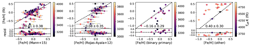
Figure 6: [Fe/H] recovery for our 3 parameter fit in $T_{\rm eff}$, [Fe/H], $m_{\rm bol}$ for our four sets of [Fe/H] standards: Mann et al. 2015, Rojas-Ayala et al. 2012, primary star [Fe/H] for cool dwarfs in binaries, and mid-K dwarfs. The median and standard deviation of each set of residuals is annotated. Note the inability of the 3 parameter fit to reliably recover [Fe/H], with the scatter on our recovered [Fe/H] for the binary sample (the most reliable set of [Fe/H] standards) being larger than the scatter on our photometric [Fe/H] relation.

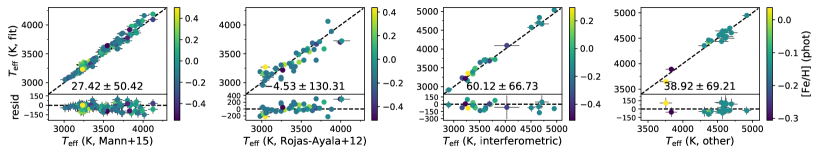
Figure 7: $T_{\rm eff}$ recovery for our 2 parameter fit in $T_{\rm eff}$, and $m_{\rm bol}$ for our four sets of $T_{\rm eff}$ standards: Mann et al. 2015, Rojas-Ayala et al. 2012, interferometry, and mid-K dwarfs. [Fe/H] is from our photometric [Fe/H] relation where appropriate, or fixed to the mean Solar Neighbourhood [Fe/H] if not. The median and standard deviation of each set of residuals is annotated (note that these values have not yet been corrected for the systematic, as discussed in Section 6.2).

Figure 8: Radius comparison for those targets with interfometric radii to better than 5% precision. The median distance precision for these targets is $0.04\,$%. We find generally good agreement between literature measurements and our own, though noting that the brightness of this sample (see apparent 2MASS $K_{S}$ magnitude on the colour bar) results in photometry that is either saturated or has lower precision and thus may be the cause of some of the scatter observed.

Table 3: Final results for TESS candidate exoplanet hosts

TOI	TIC	$T_{\rm eff}$	$\log g$	[Fe/H]	$M$	$R_{\star}$	$m_{\rm bol}$	$f_{\rm bol}$	EW(H$\alpha$)	$\log R^{{}^{\prime}}_{\rm HK}$
		(K)			($M_{\odot}$)	($R_{\odot}$)		(10${}^{-12}\,$ergs s-1 cm -2)	$\text{\,}\mathrm{\SIUnitSymbolAngstrom}$
136	410153553	2988 $\pm$ 30	5.06 $\pm$ 0.02	-	0.155 $\pm$ 0.004	0.192 $\pm$ 0.004	12.05 $\pm$ 0.01	384.4 $\pm$ 3.9	-0.05	-5.37
540	200322593	3104 $\pm$ 30	5.07 $\pm$ 0.02	-0.10	0.164 $\pm$ 0.004	0.197 $\pm$ 0.004	11.71 $\pm$ 0.01	528.3 $\pm$ 5.3	2.49	-
256	92226327	3150 $\pm$ 30	5.01 $\pm$ 0.02	-0.13	0.182 $\pm$ 0.005	0.220 $\pm$ 0.004	11.55 $\pm$ 0.01	611.8 $\pm$ 6.1	-0.22	-5.53
203	259962054	3169 $\pm$ 30	5.01 $\pm$ 0.02	-0.07	0.200 $\pm$ 0.005	0.232 $\pm$ 0.004	12.49 $\pm$ 0.01	255.4 $\pm$ 2.6	0.56	-4.98
507	348538431	3279 $\pm$ 30	4.76 $\pm$ 0.02	-	0.383 $\pm$ 0.010	0.424 $\pm$ 0.008	14.28 $\pm$ 0.01	49.2 $\pm$ 0.5	2.24	-4.49
910	369327947	3282 $\pm$ 30	4.97 $\pm$ 0.02	-0.04	0.262 $\pm$ 0.008	0.278 $\pm$ 0.005	10.46 $\pm$ 0.01	1656.2 $\pm$ 16.6	-0.27	-5.47
210	141608198	3284 $\pm$ 30	4.90 $\pm$ 0.02	0.21	0.312 $\pm$ 0.008	0.326 $\pm$ 0.006	12.78 $\pm$ 0.01	195.8 $\pm$ 2.0	-0.23	-5.84
122	231702397	3326 $\pm$ 30	4.86 $\pm$ 0.02	-0.07	0.316 $\pm$ 0.008	0.345 $\pm$ 0.006	13.42 $\pm$ 0.01	109.3 $\pm$ 1.1	-0.21	-
455	98796344	3330 $\pm$ 30	4.97 $\pm$ 0.02	-0.27	0.248 $\pm$ 0.006	0.271 $\pm$ 0.005	9.16 $\pm$ 0.01	5507.5 $\pm$ 54.8	-0.29	-5.39
732	36724087	3354 $\pm$ 30	4.83 $\pm$ 0.02	0.13	0.364 $\pm$ 0.009	0.382 $\pm$ 0.007	10.91 $\pm$ 0.01	1103.5 $\pm$ 11.0	-0.23	-5.55
674	158588995	3355 $\pm$ 30	4.77 $\pm$ 0.02	-	0.419 $\pm$ 0.010	0.443 $\pm$ 0.008	12.19 $\pm$ 0.01	338.7 $\pm$ 3.4	-0.45	-5.58
406	153065527	3369 $\pm$ 30	4.83 $\pm$ 0.02	0.21	0.380 $\pm$ 0.009	0.392 $\pm$ 0.007	11.58 $\pm$ 0.01	594.6 $\pm$ 5.9	-0.15	-5.40
175	307210830	3381 $\pm$ 30	4.94 $\pm$ 0.02	-0.24	0.293 $\pm$ 0.007	0.304 $\pm$ 0.005	9.78 $\pm$ 0.01	3099.8 $\pm$ 31.1	-0.31	-5.47
782	429358906	3390 $\pm$ 30	4.81 $\pm$ 0.02	0.25	0.401 $\pm$ 0.010	0.413 $\pm$ 0.008	12.57 $\pm$ 0.01	237.3 $\pm$ 2.4	-0.37	-6.38
244	118327550	3422 $\pm$ 30	4.82 $\pm$ 0.02	0.10	0.402 $\pm$ 0.010	0.407 $\pm$ 0.007	10.69 $\pm$ 0.01	1349.2 $\pm$ 13.5	-0.30	-5.36
789	300710077	3434 $\pm$ 30	4.86 $\pm$ 0.02	-0.16	0.360 $\pm$ 0.009	0.371 $\pm$ 0.007	12.34 $\pm$ 0.01	294.0 $\pm$ 2.9	-0.28	-
654	35009898	3436 $\pm$ 30	4.77 $\pm$ 0.02	0.07	0.425 $\pm$ 0.010	0.445 $\pm$ 0.008	12.56 $\pm$ 0.01	239.6 $\pm$ 2.4	-0.33	-8.10
864	231728511	3452 $\pm$ 30	4.82 $\pm$ 0.02	-0.10	0.392 $\pm$ 0.010	0.403 $\pm$ 0.007	11.86 $\pm$ 0.01	460.0 $\pm$ 4.6	-0.37	-5.21
562	413248763	3456 $\pm$ 30	4.88 $\pm$ 0.02	-0.22	0.347 $\pm$ 0.008	0.353 $\pm$ 0.006	9.11 $\pm$ 0.01	5758.7 $\pm$ 57.3	-0.25	-5.93
486	260708537	3467 $\pm$ 30	4.81 $\pm$ 0.02	0.03	0.424 $\pm$ 0.010	0.424 $\pm$ 0.007	9.74 $\pm$ 0.01	3239.2 $\pm$ 32.4	-0.40	-5.39
700	150428135	3467 $\pm$ 30	4.80 $\pm$ 0.02	-	0.416 $\pm$ 0.010	0.426 $\pm$ 0.007	11.28 $\pm$ 0.01	783.3 $\pm$ 7.8	-0.35	-5.36
521	27649847	3468 $\pm$ 30	4.80 $\pm$ 0.02	-0.01	0.416 $\pm$ 0.010	0.424 $\pm$ 0.008	12.74 $\pm$ 0.01	203.5 $\pm$ 2.0	-0.30	-5.49
1078	370133522	3486 $\pm$ 30	4.83 $\pm$ 0.02	-0.24	0.383 $\pm$ 0.009	0.392 $\pm$ 0.007	10.51 $\pm$ 0.01	1583.2 $\pm$ 15.8	-0.34	-6.54
912	406941612	3488 $\pm$ 30	4.80 $\pm$ 0.02	-0.03	0.424 $\pm$ 0.010	0.427 $\pm$ 0.007	10.87 $\pm$ 0.01	1143.7 $\pm$ 11.4	-0.31	-5.19
270	259377017	3493 $\pm$ 30	4.88 $\pm$ 0.02	-0.25	0.364 $\pm$ 0.009	0.361 $\pm$ 0.006	10.90 $\pm$ 0.01	1111.3 $\pm$ 11.1	-0.29	-5.40
696	77156829	3496 $\pm$ 30	4.92 $\pm$ 0.02	-0.45	0.321 $\pm$ 0.008	0.327 $\pm$ 0.006	10.84 $\pm$ 0.01	1170.5 $\pm$ 11.7	-0.22	-6.08
269	220479565	3518 $\pm$ 30	4.83 $\pm$ 0.02	-0.25	0.391 $\pm$ 0.010	0.396 $\pm$ 0.007	12.69 $\pm$ 0.01	214.2 $\pm$ 2.1	-0.30	-
233	415969908	3527 $\pm$ 30	4.88 $\pm$ 0.02	-0.31	0.371 $\pm$ 0.009	0.365 $\pm$ 0.006	11.72 $\pm$ 0.01	522.8 $\pm$ 5.2	-0.31	-5.21
698	141527579	3540 $\pm$ 30	4.76 $\pm$ 0.02	0.04	0.473 $\pm$ 0.011	0.474 $\pm$ 0.008	12.49 $\pm$ 0.01	255.5 $\pm$ 2.5	-0.39	-5.12
731	34068865	3543 $\pm$ 30	4.77 $\pm$ 0.02	-0.03	0.458 $\pm$ 0.011	0.463 $\pm$ 0.008	8.41 $\pm$ 0.01	11008.1 $\pm$ 109.5	-0.39	-5.24
1201	29960110	3546 $\pm$ 30	4.75 $\pm$ 0.02	0.11	0.484 $\pm$ 0.012	0.488 $\pm$ 0.008	11.31 $\pm$ 0.01	757.8 $\pm$ 7.6	-0.13	-4.74
756	73649615	3581 $\pm$ 30	4.71 $\pm$ 0.02	0.11	0.509 $\pm$ 0.012	0.522 $\pm$ 0.009	12.90 $\pm$ 0.01	175.4 $\pm$ 1.7	-0.42	-4.90
704	260004324	3596 $\pm$ 30	4.69 $\pm$ 0.02	-0.05	0.506 $\pm$ 0.012	0.533 $\pm$ 0.009	10.54 $\pm$ 0.01	1540.8 $\pm$ 15.4	-0.41	-5.01
177	262530407	3613 $\pm$ 30	4.70 $\pm$ 0.02	-	0.519 $\pm$ 0.013	0.532 $\pm$ 0.009	9.91 $\pm$ 0.01	2762.3 $\pm$ 27.5	0.00	-4.45
797	271596225	3618 $\pm$ 30	4.76 $\pm$ 0.02	-	0.475 $\pm$ 0.011	0.476 $\pm$ 0.008	12.13 $\pm$ 0.01	356.5 $\pm$ 3.5	-0.45	-4.92
727	149788158	3634 $\pm$ 30	4.74 $\pm$ 0.02	-0.11	0.499 $\pm$ 0.012	0.501 $\pm$ 0.008	11.42 $\pm$ 0.01	686.3 $\pm$ 6.8	-0.40	-5.02
142	425934411	3647 $\pm$ 30	4.55 $\pm$ 0.02	-	0.594 $\pm$ 0.016	0.675 $\pm$ 0.016	15.09 $\pm$ 0.01	23.4 $\pm$ 0.2	0.98	-4.25
663	54962195	3658 $\pm$ 30	4.72 $\pm$ 0.02	-0.10	0.514 $\pm$ 0.012	0.521 $\pm$ 0.009	12.18 $\pm$ 0.01	341.4 $\pm$ 3.4	-0.49	-
234	12423815	3668 $\pm$ 30	4.70 $\pm$ 0.02	0.13	0.545 $\pm$ 0.015	0.546 $\pm$ 0.013	14.99 $\pm$ 0.01	25.7 $\pm$ 0.3	-0.51	-4.97
620	296739893	3669 $\pm$ 30	4.70 $\pm$ 0.02	0.19	0.547 $\pm$ 0.014	0.547 $\pm$ 0.009	10.62 $\pm$ 0.01	1437.2 $\pm$ 14.3	-0.45	-5.07
672	151825527	3678 $\pm$ 30	4.67 $\pm$ 0.02	0.01	0.544 $\pm$ 0.013	0.563 $\pm$ 0.009	12.08 $\pm$ 0.01	375.7 $\pm$ 3.7	-0.34	-4.62
873	237920046	3682 $\pm$ 30	4.72 $\pm$ 0.02	-0.09	0.521 $\pm$ 0.013	0.519 $\pm$ 0.009	12.55 $\pm$ 0.01	243.2 $\pm$ 2.4	-0.39	-4.81
714	219195044	3698 $\pm$ 30	4.77 $\pm$ 0.02	-0.33	0.474 $\pm$ 0.011	0.468 $\pm$ 0.008	11.98 $\pm$ 0.01	410.0 $\pm$ 4.1	-0.47	-5.22
134	234994474	3722 $\pm$ 30	4.60 $\pm$ 0.02	-	0.590 $\pm$ 0.015	0.633 $\pm$ 0.010	9.65 $\pm$ 0.01	3512.5 $\pm$ 35.0	-0.47	-4.69
468	33521996	3738 $\pm$ 30	4.60 $\pm$ 0.02	-	0.588 $\pm$ 0.015	0.634 $\pm$ 0.012	13.75 $\pm$ 0.01	80.4 $\pm$ 0.8	-0.55	-4.93
785	374829238	3740 $\pm$ 30	4.67 $\pm$ 0.02	-0.02	0.559 $\pm$ 0.014	0.572 $\pm$ 0.009	11.92 $\pm$ 0.01	432.7 $\pm$ 4.3	-0.39	-4.52
552	44737596	3742 $\pm$ 30	4.65 $\pm$ 0.02	0.21	0.579 $\pm$ 0.014	0.594 $\pm$ 0.011	14.19 $\pm$ 0.01	53.6 $\pm$ 0.5	-0.42	-4.19
904	261257684	3752 $\pm$ 30	4.71 $\pm$ 0.02	-0.17	0.533 $\pm$ 0.013	0.537 $\pm$ 0.009	11.28 $\pm$ 0.01	778.7 $\pm$ 7.8	-0.39	-4.60
741	359271092	3763 $\pm$ 30	4.73 $\pm$ 0.02	-0.17	0.527 $\pm$ 0.013	0.520 $\pm$ 0.008	8.12 $\pm$ 0.01	14329.1 $\pm$ 142.6	-0.46	-5.03
198	12421862	3770 $\pm$ 30	4.86 $\pm$ 0.02	-	0.447 $\pm$ 0.011	0.413 $\pm$ 0.007	10.39 $\pm$ 0.01	1769.6 $\pm$ 17.7	-0.42	-5.14
442	70899085	3831 $\pm$ 30	4.63 $\pm$ 0.02	0.09	0.598 $\pm$ 0.015	0.620 $\pm$ 0.010	11.17 $\pm$ 0.01	867.7 $\pm$ 8.6	-0.40	-4.53
557	55488511	3845 $\pm$ 30	4.67 $\pm$ 0.02	-0.15	0.570 $\pm$ 0.014	0.581 $\pm$ 0.009	12.09 $\pm$ 0.01	371.3 $\pm$ 3.7	-0.51	-4.69
870	219229644	3847 $\pm$ 30	4.63 $\pm$ 0.02	0.11	0.601 $\pm$ 0.015	0.618 $\pm$ 0.010	11.21 $\pm$ 0.01	836.3 $\pm$ 8.3	-0.38	-4.54
551	192826603	3871 $\pm$ 30	4.67 $\pm$ 0.02	-0.28	0.563 $\pm$ 0.014	0.577 $\pm$ 0.010	14.35 $\pm$ 0.01	46.4 $\pm$ 0.5	-0.54	-4.60
876	32497972	3888 $\pm$ 30	4.63 $\pm$ 0.02	-0.08	0.595 $\pm$ 0.015	0.615 $\pm$ 0.010	11.98 $\pm$ 0.01	410.9 $\pm$ 4.1	-0.55	-4.85
532	144700903	3903 $\pm$ 30	4.62 $\pm$ 0.02	0.07	0.610 $\pm$ 0.015	0.630 $\pm$ 0.011	13.09 $\pm$ 0.01	147.8 $\pm$ 1.5	-0.68	-5.39
1075	351601843	3916 $\pm$ 30	4.69 $\pm$ 0.02	-	0.575 $\pm$ 0.014	0.571 $\pm$ 0.009	11.59 $\pm$ 0.01	588.2 $\pm$ 5.9	-0.50	-4.66
833	362249359	3945 $\pm$ 30	4.65 $\pm$ 0.02	-0.13	0.595 $\pm$ 0.015	0.601 $\pm$ 0.009	10.60 $\pm$ 0.01	1458.0 $\pm$ 14.5	-0.49	-4.49
702	237914496	3966 $\pm$ 30	4.69 $\pm$ 0.02	-0.24	0.577 $\pm$ 0.014	0.566 $\pm$ 0.009	12.24 $\pm$ 0.01	323.3 $\pm$ 3.2	-0.56	-4.65
555	170849515	3993 $\pm$ 30	4.63 $\pm$ 0.02	-0.06	0.615 $\pm$ 0.017	0.626 $\pm$ 0.015	15.25 $\pm$ 0.01	20.1 $\pm$ 0.2	-0.40	-4.76
285	220459976	3995 $\pm$ 30	4.62 $\pm$ 0.02	0.00	0.625 $\pm$ 0.015	0.643 $\pm$ 0.010	12.61 $\pm$ 0.01	229.2 $\pm$ 2.3	-0.60	-4.71
475	100608026	4003 $\pm$ 30	4.66 $\pm$ 0.02	-0.18	0.601 $\pm$ 0.015	0.599 $\pm$ 0.009	11.29 $\pm$ 0.01	775.1 $\pm$ 7.7	-0.54	-4.62
253	322063810	4039 $\pm$ 30	4.65 $\pm$ 0.02	-	0.617 $\pm$ 0.015	0.618 $\pm$ 0.009	9.79 $\pm$ 0.01	3087.3 $\pm$ 30.8	-0.60	-4.87
435	44647437	4079 $\pm$ 30	4.64 $\pm$ 0.02	-0.13	0.621 $\pm$ 0.015	0.627 $\pm$ 0.010	13.34 $\pm$ 0.01	116.9 $\pm$ 1.2	-0.56	-4.57

Table 4: continued

Final results for TESS candidate exoplanet hosts TOI TIC $T_{\rm eff}$ $\log g$ [Fe/H] $M$ $R_{\star}$ $m_{\rm bol}$ $f_{\rm bol}$ EW(H$\alpha$) $\log R^{{}^{\prime}}_{\rm HK}$ (K) ($M_{\odot}$) ($R_{\odot}$) (10${}^{-12}\,$ergs s^-1 cm ^-2) $\text{\,}\mathrm{\SIUnitSymbolAngstrom}$ 1082 261108236 4096 $\pm$ 30 4.65 $\pm$ 0.02 -0.24 0.610 $\pm$ 0.015 0.609 $\pm$ 0.009 12.31 $\pm$ 0.01 302.8 $\pm$ 3.0 -0.61 -4.76 260 37749396 4097 $\pm$ 30 4.70 $\pm$ 0.02 -0.28 0.598 $\pm$ 0.015 0.575 $\pm$ 0.009 8.96 $\pm$ 0.01 6614.9 $\pm$ 65.9 -0.60 -4.75 761 165317334 4121 $\pm$ 30 4.64 $\pm$ 0.02 -0.15 0.623 $\pm$ 0.015 0.629 $\pm$ 0.010 11.34 $\pm$ 0.01 740.9 $\pm$ 7.4 -0.60 -4.49 249 179985715 4128 $\pm$ 30 4.71 $\pm$ 0.02 - 0.589 $\pm$ 0.015 0.561 $\pm$ 0.008 11.70 $\pm$ 0.01 531.3 $\pm$ 5.3 -0.56 -4.61 806 33831980 4137 $\pm$ 30 4.68 $\pm$ 0.02 -0.29 0.607 $\pm$ 0.015 0.592 $\pm$ 0.009 12.42 $\pm$ 0.01 274.5 $\pm$ 2.7 -0.62 -4.65 1216 141527965 4217 $\pm$ 30 4.61 $\pm$ 0.02 -0.13 0.649 $\pm$ 0.016 0.664 $\pm$ 0.010 11.98 $\pm$ 0.01 410.5 $\pm$ 4.1 -0.67 -4.68 302 229111835 4227 $\pm$ 30 4.59 $\pm$ 0.02 -0.03 0.661 $\pm$ 0.016 0.684 $\pm$ 0.011 13.36 $\pm$ 0.01 115.2 $\pm$ 1.2 -0.73 -4.60 656 36734222 4241 $\pm$ 30 4.58 $\pm$ 0.02 -0.07 0.662 $\pm$ 0.016 0.690 $\pm$ 0.010 11.57 $\pm$ 0.01 595.9 $\pm$ 6.0 -0.61 -4.46 1130 254113311 4275 $\pm$ 30 4.55 $\pm$ 0.02 -0.12 0.670 $\pm$ 0.017 0.716 $\pm$ 0.011 10.60 $\pm$ 0.01 1463.9 $\pm$ 14.6 -0.73 -4.78 133 219338557 4276 $\pm$ 30 4.64 $\pm$ 0.02 -0.22 0.646 $\pm$ 0.016 0.639 $\pm$ 0.009 10.45 $\pm$ 0.01 1673.5 $\pm$ 16.7 -0.71 -5.06 544 50618703 4292 $\pm$ 30 4.66 $\pm$ 0.02 -0.24 0.641 $\pm$ 0.016 0.623 $\pm$ 0.009 10.13 $\pm$ 0.01 2253.9 $\pm$ 22.4 -0.64 -4.56 836 440887364 4308 $\pm$ 30 4.62 $\pm$ 0.02 -0.15 0.658 $\pm$ 0.016 0.659 $\pm$ 0.009 9.12 $\pm$ 0.01 5710.9 $\pm$ 56.9 -0.68 -4.61 240 101948569 4333 $\pm$ 30 4.59 $\pm$ 0.02 - 0.676 $\pm$ 0.017 0.693 $\pm$ 0.010 11.16 $\pm$ 0.01 876.1 $\pm$ 8.8 -0.68 -4.60 713 167600516 4340 $\pm$ 30 4.64 $\pm$ 0.02 -0.25 0.648 $\pm$ 0.016 0.637 $\pm$ 0.009 11.17 $\pm$ 0.01 868.0 $\pm$ 8.7 -0.74 -5.09 900 210873792 4347 $\pm$ 30 4.63 $\pm$ 0.02 -0.23 0.653 $\pm$ 0.016 0.649 $\pm$ 0.010 12.32 $\pm$ 0.01 300.0 $\pm$ 3.0 -0.71 -5.46 493 19025965 4360 $\pm$ 30 4.59 $\pm$ 0.02 -0.05 0.677 $\pm$ 0.017 0.690 $\pm$ 0.010 11.92 $\pm$ 0.01 434.7 $\pm$ 4.3 -0.73 -4.87 178 251848941 4366 $\pm$ 30 4.64 $\pm$ 0.02 - 0.649 $\pm$ 0.016 0.639 $\pm$ 0.009 10.91 $\pm$ 0.01 1095.3 $\pm$ 10.9 -0.75 -4.85 875 14165625 4404 $\pm$ 30 4.59 $\pm$ 0.02 -0.13 0.675 $\pm$ 0.017 0.689 $\pm$ 0.010 11.85 $\pm$ 0.01 463.0 $\pm$ 4.6 -0.69 -4.57 711 38510224 4433 $\pm$ 30 4.64 $\pm$ 0.02 - 0.653 $\pm$ 0.016 0.638 $\pm$ 0.009 12.22 $\pm$ 0.01 327.6 $\pm$ 3.3 -0.73 -4.77 139 62483237 4434 $\pm$ 30 4.61 $\pm$ 0.02 - 0.673 $\pm$ 0.016 0.674 $\pm$ 0.009 9.88 $\pm$ 0.01 2827.2 $\pm$ 28.2 -0.69 -4.47 1073 158297421 4481 $\pm$ 30 4.62 $\pm$ 0.02 - 0.666 $\pm$ 0.017 0.664 $\pm$ 0.014 14.09 $\pm$ 0.01 58.6 $\pm$ 0.6 -0.69 -4.60 929 175532955 4482 $\pm$ 30 4.59 $\pm$ 0.02 - 0.684 $\pm$ 0.017 0.693 $\pm$ 0.010 11.92 $\pm$ 0.01 432.7 $\pm$ 4.3 -0.79 -10.15 969 280437559 4503 $\pm$ 30 4.59 $\pm$ 0.02 - 0.682 $\pm$ 0.017 0.693 $\pm$ 0.010 11.06 $\pm$ 0.01 960.4 $\pm$ 9.6 -0.72 -4.60 932 260417932 4508 $\pm$ 30 4.58 $\pm$ 0.02 - 0.689 $\pm$ 0.017 0.705 $\pm$ 0.010 11.23 $\pm$ 0.01 817.5 $\pm$ 8.1 -0.80 -5.22 1067 201642601 4510 $\pm$ 30 4.57 $\pm$ 0.02 - 0.698 $\pm$ 0.018 0.721 $\pm$ 0.012 13.61 $\pm$ 0.01 91.7 $\pm$ 0.9 -0.76 - 279 122613513 4512 $\pm$ 30 4.61 $\pm$ 0.02 - 0.677 $\pm$ 0.017 0.673 $\pm$ 0.009 11.03 $\pm$ 0.01 986.9 $\pm$ 9.8 -0.76 -4.61 129 201248411 4569 $\pm$ 30 4.57 $\pm$ 0.02 - 0.697 $\pm$ 0.018 0.721 $\pm$ 0.010 10.42 $\pm$ 0.01 1721.3 $\pm$ 17.2 -0.77 -4.50 824 193641523 4589 $\pm$ 30 4.60 $\pm$ 0.02 - 0.688 $\pm$ 0.018 0.691 $\pm$ 0.009 10.57 $\pm$ 0.01 1505.7 $\pm$ 15.0 -0.81 -4.76

5 Candidate Planet Parameters

5.1 Transit Light Curve Analysis

We now present results for all TOIs not ruled out as false positives (e.g. due to background stars, or eclipsing binaries) by the TESS Team and exoplanet community, as listed on the NASA ExoFOP-TESS website.

Transit light curves for targets across all TESS sectors were downloaded from NASA’s Mikulski Archive for Space Telescopes (MAST) service. For all high-cadence data, we used the Pre-search Data Conditioning Simple Aperture Photometry (PDCSAP) fluxes, which have already had some measure of processing to remove systematics.

All light curves were downloaded and manipulated using the python package LightKurve (Lightkurve Collaboration et al., 2018).

Many stars in our sample show some amount of stellar variability, with periods ranging from days to many weeks. We remove this using LightKurve’s flatten function, which applies a Savitzky-Golay filter (Savitzky & Golay, 1964) to the data to remove low frequency trends. When applying the filter we mask out all planetary transits by known TOIs. Once flattened, the light curves are then phase folded using either the period provided by NASA ExoFOP-TESS (for most stars), or our own fitted period (for stars revisited in the TESS extended mission whose long time baseline reveals the ExoFOP-TESS period to be incorrect). We use the provided measurement of transit duration to select only photometry from the transit itself, plus 10% of a duration either side for use in model fitting.

Model fitting is implemented using the python package BATMAN (Kreidberg, 2015), which is capable of generating model transit light curves for a given set of orbital elements (scaled by the stellar radius $R_{\star}$) and limb darkening coefficients. We use a four term limb darkening law, interpolating the PHOENIX grid provided by Claret (2017) using values of $T_{\rm eff}$ and $\log g$ from Table 3. The resulting coefficients are in Table 17.

Transit photometry alone is not sufficient to uniquely constrain the planet orbit and radius when fitting for the scaled semi-major axis $a_{R_{\star}}=\frac{a}{R_{\star}}$, the planetary radius ratio $R_{P,R_{\star}}=\frac{R_{P}}{R_{\star}}$, the inclination $i$, the eccentricity $e$, and the longitude of periastron $\omega$ (Kipping, 2008). While we can use our measurements of $M_{\star}$, $R_{\star}$, and $T$ to constrain the semi-major axis of a circular orbit (Equation 7), we do not have the precision required to fit for eccentric orbits. As such, we fix $e=0$ and $\omega=0$ during our fit, and include our calculated value $a_{R_{\star},c}$ - the value $a_{R_{\star}}$ assuming a circular orbit, as a prior during fitting. In cases where $e\sim 0$, we expect the fitted semi-major axis $a_{R_{\star},f}$ to approach $a_{R_{\star},c}$. For cases with a discrepancy between the two, we flag the planet as an indication of a possibly eccentric orbit in Table 5.

This measured semi-major axis, calculated using our Mann et al. (2015) absolute $K_{S}$ band $M_{\star}$, and $T$ from NASA ExoFOP, can be constrained as follows:

$$a=\sqrt[3]{\frac{GM_{\star}T^{2}}{4\pi^{2}}}$$ (7)

where $a$ is the semi-major axis, $G$ is the gravitational constant, $M_{\star}$ is the stellar mass (with $M_{\star}>>M_{p}$, the planetary mass), and $T$ is the planet orbital period - all of which we assume are independent quantities.

Now with a prior on the semi-major axis, we again use the least_squares function from scipy’s optimize module to perform least squares fitting to minimise the following expression:

$$R_{t}=\Bigg{(}\frac{{a_{R_{\star},m}-a_{R_{\star},f}}}{\sigma_{a_{R_{\star},m}}}+\displaystyle\sum_{j}^{N}\frac{{t_{\rm obs,~{}j}-t_{\rm model,~{}j}}}{\sigma_{t_{\rm obs,~{}j}}}\Bigg{)}^{2}$$ (8)

where $R_{t}$ are the light curve and prior residuals (as a function of $R_{p,R_{\star}}$, $a_{R_{\star},f}$, and $i$), $a_{R_{\star},m}$ the measured scaled semi-major axis, $a_{R_{\star},f}$ the fitted scaled semi-major axis, $\sigma_{a_{R_{\star},m}}$ the uncertainty on the measured scaled semi-major axis, $j$ is the time step, $N$ the total number of epochs, $t_{\rm obs,~{}j}$ is the observed flux at time step $j$, $t_{\rm model,~{}j}$ the model flux at time step $j$, and $\sigma_{t_{\rm obs,~{}j}}$ is the measured flux uncertainty at time step $j$.

Results from this fitting procedure are presented in Table 5, a comparison with confirmed planets in Figure 11, and a histogram of the resulting planet candidate radii in Figure 12. Note that we do not fit the light curves for some candidates: TOIs 256.01 and 415969908.02 have only two and one transits respectively; TOI 507.01 is a suspected equal mass binary; TOIs 302.01 and 969.01 do not have PDCSAP two minute cadence data; and TOIs 203.01, 253.01, 285.01, 696.02, 785.01, 864.01, 1216.01, 260417932.02, and 98796344.02 have transits observed only at low SNR.

Table 5: Final results for TESS candidate exoplanets.

TOI	TIC	Sector/s	Period	$R_{p}/R_{\star}$	$a/R_{\star}$	$e$ flag	$i$	$R_{p}$
			(days)				(∘)	($R_{\oplus}$)
122.01	231702397	1,27-28	5.07803 $\dagger$	0.0797 $\pm$ 0.0022	24.63 $\pm$ 0.49	0	88.337 $\pm$ 0.001	3.00 $\pm$ 0.10
129.01	201248411	1-2,28-29	0.98097 $\dagger$	0.3223 $\pm$ 0.0884	5.15 $\pm$ 0.04	0	76.381 $\pm$ 0.018	25.35 $\pm$ 6.96
133.01	219338557	1,28	8.19918 $\dagger$	0.0269 $\pm$ 0.0010	23.15 $\pm$ 0.41	0	88.470 $\pm$ 0.002	1.88 $\pm$ 0.07
134.01	234994474	1,28	1.40153 $\dagger$	0.0223 $\pm$ 0.0006	6.98 $\pm$ 0.16	0	84.566 $\pm$ 0.005	1.54 $\pm$ 0.05
136.01	410153553	1,27-28	0.46293 $\dagger$	0.0587 $\pm$ 0.0006	6.80 $\pm$ 0.17	1	90.000 $\pm$ 5.000	1.23 $\pm$ 0.03
139.01	62483237	1,28	11.07083 $\dagger$	0.0346 $\pm$ 0.0008	27.20 $\pm$ 0.56	0	88.549 $\pm$ 0.001	2.54 $\pm$ 0.07
142.01	425934411	1-2,28-29	0.85335 $\dagger$	0.1809 $\pm$ 0.0184	4.74 $\pm$ 0.11	0	79.385 $\pm$ 0.012	13.31 $\pm$ 1.39
175.01	307210830	2,5,8-12,28-29,32	3.69066 $\dagger$	0.0397 $\pm$ 0.0003	21.32 $\pm$ 0.47	0	88.809 $\pm$ 0.002	1.32 $\pm$ 0.03
175.02	307210830	2,5,8-12,28-29,32	7.45075 $\dagger$	0.0446 $\pm$ 0.0006	34.59 $\pm$ 0.75	0	88.483 $\pm$ 0.001	1.48 $\pm$ 0.03
175.03	307210830	2,5,8-12,28-29,32	2.25310 $\dagger$	0.0238 $\pm$ 0.0003	15.76 $\pm$ 0.34	0	88.133 $\pm$ 0.003	0.79 $\pm$ 0.02
177.01	262530407	2-3,29	2.85310 $\dagger$	0.0385 $\pm$ 0.0005	12.70 $\pm$ 0.26	0	86.765 $\pm$ 0.002	2.24 $\pm$ 0.05
178.01	251848941	2,29	6.55770 $\dagger$	0.0365 $\pm$ 0.0009	19.97 $\pm$ 0.36	0	88.506 $\pm$ 0.002	2.54 $\pm$ 0.07
178.02	251848941	2,29	20.70950 $\dagger$	0.0439 $\pm$ 0.0023	42.94 $\pm$ 0.70	0	88.821 $\pm$ 0.001	3.06 $\pm$ 0.16
178.03	251848941	2,29	9.96188 $\dagger$	0.0252 $\pm$ 0.0013	26.40 $\pm$ 0.45	0	88.855 $\pm$ 0.002	1.76 $\pm$ 0.09
178 b	251848941	2,29	1.91456 $\dagger$	0.0197 $\pm$ 0.0008	8.78 $\pm$ 0.15	0	89.745 $\pm$ 0.094	1.37 $\pm$ 0.06
178 c	251848941	2,29	3.23845 $\dagger$	0.0231 $\pm$ 0.0008	12.47 $\pm$ 0.22	0	88.423 $\pm$ 0.007	1.61 $\pm$ 0.06
178 f	251848941	2,29	15.23191 $\dagger$	0.0314 $\pm$ 0.0011	35.01 $\pm$ 0.59	0	88.904 $\pm$ 0.001	2.19 $\pm$ 0.08
198.01	12421862	2,29	20.43021 $\dagger$	0.0291 $\pm$ 0.0012	58.19 $\pm$ 1.14	0	89.374 $\pm$ 0.001	1.31 $\pm$ 0.06
210.01	141608198	1-5,7-13,27-32	9.01056 $\dagger$	0.0629 $\pm$ 0.0007	37.78 $\pm$ 0.66	0	89.531 $\pm$ 0.002	2.24 $\pm$ 0.05
233.01	415969908	2,29	11.66993 $\dagger$	0.0457 $\pm$ 0.0013	42.65 $\pm$ 0.82	0	89.606 $\pm$ 0.002	1.82 $\pm$ 0.06
234.01	12423815	2,29	2.83927 $\dagger$	0.1932 $\pm$ 0.0045	12.63 $\pm$ 0.28	0	86.641 $\pm$ 0.003	11.50 $\pm$ 0.39
240.01	101948569	2,29	19.47241 $\dagger$	0.0388 $\pm$ 0.0013	38.59 $\pm$ 0.59	0	89.278 $\pm$ 0.001	2.93 $\pm$ 0.10
244.01	118327550	2,29	7.39719 $\dagger$	0.0321 $\pm$ 0.0012	29.05 $\pm$ 0.56	0	88.382 $\pm$ 0.001	1.42 $\pm$ 0.06
249.01	179985715	2,29	6.61542 $\dagger$	0.0329 $\pm$ 0.0018	22.18 $\pm$ 0.38	0	88.757 $\pm$ 0.003	2.01 $\pm$ 0.11
256.02	92226327	3,30	3.77796 $\dagger$	0.0480 $\pm$ 0.0010	25.61 $\pm$ 0.59	0	90.000 $\pm$ 5.000	1.15 $\pm$ 0.03
260.01	37749396	3	13.470018	0.0265 $\pm$ 0.0010	34.87 $\pm$ 0.60	0	88.758 $\pm$ 0.001	1.66 $\pm$ 0.07
269.01	220479565	3-6,10,13,30-32	3.69770 $\dagger$	0.0691 $\pm$ 0.0012	18.65 $\pm$ 0.31	0	87.384 $\pm$ 0.001	2.99 $\pm$ 0.07
270.01	259377017	3-5,30,32	5.66054 $\dagger$	0.0581 $\pm$ 0.0004	26.06 $\pm$ 0.55	0	89.210 $\pm$ 0.002	2.29 $\pm$ 0.04
270.02	259377017	3-5,30,32	11.37960 $\dagger$	0.0535 $\pm$ 0.0004	41.87 $\pm$ 0.78	0	89.707 $\pm$ 0.002	2.11 $\pm$ 0.04
270.03	259377017	3-5,30,32	3.36014 $\dagger$	0.0301 $\pm$ 0.0005	18.65 $\pm$ 0.37	0	89.218 $\pm$ 0.005	1.18 $\pm$ 0.03
279.01	122613513	3-4	11.494122	0.0361 $\pm$ 0.0013	27.95 $\pm$ 0.45	0	88.583 $\pm$ 0.001	2.65 $\pm$ 0.10
406.01	153065527	3-4,30-31	13.17573 $\dagger$	0.0430 $\pm$ 0.0013	43.35 $\pm$ 0.87	0	89.303 $\pm$ 0.001	1.84 $\pm$ 0.06
435.01	44647437	4-5,31	3.35293 $\dagger$	0.0583 $\pm$ 0.0016	12.82 $\pm$ 0.23	0	88.622 $\pm$ 0.007	3.99 $\pm$ 0.12
442.01	70899085	5,32	4.05203 $\dagger$	0.0741 $\pm$ 0.0007	14.48 $\pm$ 0.25	0	86.865 $\pm$ 0.002	5.02 $\pm$ 0.09
455.01	98796344	4,31	5.35880 $\dagger$	0.0467 $\pm$ 0.0009	29.82 $\pm$ 1.22	0	89.391 $\pm$ 0.005	1.38 $\pm$ 0.04
468.01	33521996	6,32	3.32527 $\dagger$	0.1735 $\pm$ 0.0014	12.63 $\pm$ 0.25	0	87.382 $\pm$ 0.003	12.01 $\pm$ 0.24
475.01	100608026	5-6,32	8.26159 $\dagger$	0.0307 $\pm$ 0.0014	24.22 $\pm$ 0.42	0	89.006 $\pm$ 0.003	2.00 $\pm$ 0.10
486.01	260708537	1-6,8-13,27-32	1.74468 $\dagger$	0.0128 $\pm$ 0.0003	10.82 $\pm$ 0.21	0	88.585 $\pm$ 0.008	0.59 $\pm$ 0.02
493.01	19025965	7	5.947773	0.0518 $\pm$ 0.0020	17.60 $\pm$ 0.25	0	87.987 $\pm$ 0.003	3.90 $\pm$ 0.16
521.01	27649847	7	1.542131	0.0463 $\pm$ 0.0028	9.89 $\pm$ 0.17	0	86.478 $\pm$ 0.006	2.15 $\pm$ 0.14
532.01	144700903	6	2.326811	0.0876 $\pm$ 0.0020	9.96 $\pm$ 0.14	0	87.050 $\pm$ 0.004	6.02 $\pm$ 0.17
540.01	200322593	4-6,31-32	1.23914 $\dagger$	0.0366 $\pm$ 0.0010	13.48 $\pm$ 0.32	0	87.063 $\pm$ 0.003	0.78 $\pm$ 0.03
544.01	50618703	6,32	1.54835 $\dagger$	0.0281 $\pm$ 0.0006	7.80 $\pm$ 0.14	0	85.103 $\pm$ 0.004	1.91 $\pm$ 0.05
551.01	192826603	5-6,32	2.64730 $\dagger$	0.3387 $\pm$ 1.1540	11.60 $\pm$ 0.17	0	84.411 $\pm$ 0.118	21.32 $\pm$ 72.62
552.01	44737596	4-5,31	2.78864 $\dagger$	0.1552 $\pm$ 0.0014	11.57 $\pm$ 0.19	0	87.675 $\pm$ 0.003	10.05 $\pm$ 0.20
555.01	170849515	5,31-32	1.94163 $\dagger$	0.1548 $\pm$ 0.0028	8.92 $\pm$ 0.20	0	87.380 $\pm$ 0.008	10.57 $\pm$ 0.32
557.01	55488511	5,31	3.34499 $\dagger$	0.0388 $\pm$ 0.0025	13.43 $\pm$ 0.21	0	86.264 $\pm$ 0.002	2.46 $\pm$ 0.16
562.01	413248763	8	3.930792	0.0329 $\pm$ 0.0007	20.86 $\pm$ 0.41	0	88.691 $\pm$ 0.002	1.27 $\pm$ 0.03
620.01	296739893	8	5.098373	0.0597 $\pm$ 0.0015	18.65 $\pm$ 0.35	0	87.394 $\pm$ 0.001	3.56 $\pm$ 0.11
654.01	35009898	9	1.527419	0.0513 $\pm$ 0.0019	9.44 $\pm$ 0.16	0	87.873 $\pm$ 0.010	2.49 $\pm$ 0.10
656.01	36734222	9	0.813470	0.1608 $\pm$ 0.0005	4.67 $\pm$ 0.03	0	81.396 $\pm$ 0.002	12.11 $\pm$ 0.19
663.01	54962195	9	2.598654	0.0408 $\pm$ 0.0017	12.24 $\pm$ 0.17	0	88.685 $\pm$ 0.010	2.32 $\pm$ 0.11
663.02	54962195	9	4.698465	0.0433 $\pm$ 0.0023	18.16 $\pm$ 0.25	0	88.488 $\pm$ 0.004	2.46 $\pm$ 0.14
672.01	151825527	9-10	3.633618	0.0889 $\pm$ 0.0008	14.44 $\pm$ 0.20	0	87.932 $\pm$ 0.002	5.45 $\pm$ 0.10
674.01	158588995	9-10	1.977238	0.1174 $\pm$ 0.0009	11.35 $\pm$ 0.17	0	86.352 $\pm$ 0.002	5.67 $\pm$ 0.11
696.01	77156829	4-5,31-32	0.86024 $\dagger$	0.0221 $\pm$ 0.0008	7.96 $\pm$ 0.16	0	84.721 $\pm$ 0.004	0.79 $\pm$ 0.03
698.01	141527579	1-5,7-13,27-32	15.08666 $\dagger$	0.0436 $\pm$ 0.0010	42.17 $\pm$ 0.68	0	89.058 $\pm$ 0.001	2.26 $\pm$ 0.07
700.01	150428135	1,3-11,13,27-28,30-31	16.05110 $\dagger$	0.0573 $\pm$ 0.0010	47.21 $\pm$ 0.89	0	88.902 $\pm$ 0.000	2.66 $\pm$ 0.07
700.02	150428135	1,3-11,13,27-28,30-31	37.42475 $\dagger$	0.0272 $\pm$ 0.0008	82.17 $\pm$ 1.66	0	90.000 $\pm$ 5.307	1.26 $\pm$ 0.04
700.03	150428135	1,3-11,13,27-28,30-31	9.97701 $\dagger$	0.0181 $\pm$ 0.0009	34.16 $\pm$ 0.66	0	89.885 $\pm$ 0.014	0.84 $\pm$ 0.04

Notes: Periods denoted by $\dagger$ are not as reported by ExoFOP, and have been refitted here. These are overwhelmingly systems with TESS extended mission data, thus having longer time baselines with which to constrain orbital periods. Our fitted periods however are generally consistent within uncertainties of their ExoFOP values, and as such we do not report new uncertainties here. Additionally, our least squares fits to 7 of our light curves proved insenstive to non-edge-on inclinations. As such, we report conservative uncertanties of $\pm 5$°  for these planets.

Table 6: continued

Final results for TESS candidate exoplanets TOI TIC Sector/s Period $R_{p}/R_{\star}$ $a/R_{\star}$ $e$ flag $i$ $R_{p}$ (days) (^∘) ($R_{\oplus}$) 702.01 237914496 1-4,7,11,27,29-31 3.56809 $\dagger$ 0.0280 $\pm$ 0.0010 14.46 $\pm$ 0.24 0 87.421 $\pm$ 0.002 1.73 $\pm$ 0.07 704.01 260004324 1-5,7-13,27-32 3.81431 $\dagger$ 0.0208 $\pm$ 0.0004 15.38 $\pm$ 0.28 0 87.419 $\pm$ 0.002 1.21 $\pm$ 0.03 711.01 38510224 1-5,7-8,11-12,28-32 18.38384 $\dagger$ 0.0301 $\pm$ 0.0012 39.90 $\pm$ 0.64 0 89.221 $\pm$ 0.001 2.09 $\pm$ 0.09 713.01 167600516 1-8,10-13,27-32 35.99988 $\dagger$ 0.0315 $\pm$ 0.0006 62.37 $\pm$ 0.95 0 89.724 $\pm$ 0.001 2.19 $\pm$ 0.05 713.02 167600516 1-8,10-13,27-32 1.87150 $\dagger$ 0.0155 $\pm$ 0.0007 8.69 $\pm$ 0.13 0 84.872 $\pm$ 0.003 1.07 $\pm$ 0.05 714.01 219195044 4-8,11-12,28,31-32 4.32378 $\dagger$ 0.0260 $\pm$ 0.0010 18.59 $\pm$ 0.31 0 88.556 $\pm$ 0.003 1.33 $\pm$ 0.06 714.02 219195044 4-8,11-12,28,31-32 10.17742 $\dagger$ 0.0307 $\pm$ 0.0011 32.90 $\pm$ 0.51 0 89.108 $\pm$ 0.001 1.57 $\pm$ 0.06 727.01 149788158 8 4.726090 0.0293 $\pm$ 0.0020 18.76 $\pm$ 0.31 0 89.435 $\pm$ 0.014 1.60 $\pm$ 0.11 731.01 34068865 9 0.321941 0.0133 $\pm$ 0.0005 3.29 $\pm$ 0.07 0 85.081 $\pm$ 0.031 0.67 $\pm$ 0.03 732.01 36724087 9 0.768418 0.0311 $\pm$ 0.0011 6.59 $\pm$ 0.13 0 90.000 $\pm$ 5.000 1.30 $\pm$ 0.05 732.02 36724087 9 12.254218 0.0607 $\pm$ 0.0022 41.84 $\pm$ 0.74 0 88.868 $\pm$ 0.001 2.53 $\pm$ 0.10 741.01 359271092 9-10 7.576262 0.0160 $\pm$ 0.0009 25.25 $\pm$ 0.62 0 88.472 $\pm$ 0.002 0.91 $\pm$ 0.05 756.01 73649615 10-11 1.23952 $\dagger$ 0.0548 $\pm$ 0.0019 7.43 $\pm$ 0.10 0 85.039 $\pm$ 0.005 3.12 $\pm$ 0.12 761.01 165317334 10 10.563348 0.0417 $\pm$ 0.0016 27.53 $\pm$ 0.41 0 89.196 $\pm$ 0.003 2.86 $\pm$ 0.12 782.01 429358906 10 16.047203 0.0659 $\pm$ 0.0040 47.81 $\pm$ 0.69 0 89.070 $\pm$ 0.001 2.97 $\pm$ 0.19 789.01 300710077 1-3,5-13,27-32 5.44693 $\dagger$ 0.0274 $\pm$ 0.0011 24.99 $\pm$ 0.44 0 89.127 $\pm$ 0.003 1.11 $\pm$ 0.05 797.01 271596225 1-13,27-32 1.80078 $\dagger$ 0.0256 $\pm$ 0.0006 10.21 $\pm$ 0.17 0 86.580 $\pm$ 0.003 1.33 $\pm$ 0.04 797.02 271596225 1-13,27-32 4.14002 $\dagger$ 0.0292 $\pm$ 0.0011 17.78 $\pm$ 0.30 0 87.236 $\pm$ 0.001 1.52 $\pm$ 0.06 806.01 33831980 1-3,5-6,8-9,12-13,27-29,32 21.91625 $\dagger$ 0.0347 $\pm$ 0.0011 47.14 $\pm$ 0.66 0 89.479 $\pm$ 0.001 2.24 $\pm$ 0.08 824.01 193641523 11-12 1.392930 0.0436 $\pm$ 0.0007 6.69 $\pm$ 0.10 0 83.665 $\pm$ 0.004 3.29 $\pm$ 0.07 833.01 362249359 9-11 1.042241 0.0190 $\pm$ 0.0007 6.02 $\pm$ 0.10 0 89.977 $\pm$ 1.790 1.24 $\pm$ 0.05 836.01 440887364 11 8.593935 0.0346 $\pm$ 0.0006 23.32 $\pm$ 0.30 0 88.727 $\pm$ 0.001 2.49 $\pm$ 0.06 836.02 440887364 11 3.817115 0.0240 $\pm$ 0.0008 13.59 $\pm$ 0.23 0 87.727 $\pm$ 0.003 1.72 $\pm$ 0.06 870.01 219229644 3-5,30-32 22.03813 $\dagger$ 0.0330 $\pm$ 0.0012 45.25 $\pm$ 0.81 0 89.013 $\pm$ 0.001 2.22 $\pm$ 0.09 873.01 237920046 1-4,11,28-31 5.93122 $\dagger$ 0.0279 $\pm$ 0.0012 21.26 $\pm$ 0.38 0 90.000 $\pm$ 5.000 1.58 $\pm$ 0.07 875.01 14165625 5-6 11.020153 0.0277 $\pm$ 0.0021 26.47 $\pm$ 0.36 0 90.000 $\pm$ 5.000 2.08 $\pm$ 0.16 876.01 32497972 5-6,32 38.69629 $\dagger$ 0.0367 $\pm$ 0.0044 65.85 $\pm$ 1.39 0 89.254 $\pm$ 0.001 2.46 $\pm$ 0.30 900.01 210873792 12 4.844050 0.0426 $\pm$ 0.0026 15.81 $\pm$ 0.26 0 90.000 $\pm$ 5.000 3.01 $\pm$ 0.19 904.01 261257684 12-13 18.35654 $\dagger$ 0.0342 $\pm$ 0.0017 43.55 $\pm$ 0.79 0 90.000 $\pm$ 5.000 2.00 $\pm$ 0.10 910.01 369327947 12-13,27 2.02911 $\dagger$ 0.0311 $\pm$ 0.0007 15.53 $\pm$ 0.31 0 87.229 $\pm$ 0.002 0.94 $\pm$ 0.03 912.01 406941612 12-13 4.679100 0.0414 $\pm$ 0.0008 20.71 $\pm$ 0.32 0 88.819 $\pm$ 0.002 1.93 $\pm$ 0.05 929.01 175532955 30-31 5.83010 $\dagger$ 0.0314 $\pm$ 0.0015 17.32 $\pm$ 0.28 0 89.396 $\pm$ 0.012 2.37 $\pm$ 0.12 932.01 260417932 28-29,31-32 19.310700 0.0337 $\pm$ 0.0009 38.00 $\pm$ 0.62 0 89.463 $\pm$ 0.002 2.59 $\pm$ 0.08 1067.01 201642601 13,27 3.13167 $\dagger$ 0.1071 $\pm$ 0.0012 11.13 $\pm$ 0.20 0 89.174 $\pm$ 0.012 8.42 $\pm$ 0.17 1073.01 158297421 13,27 3.92282 $\dagger$ 0.1799 $\pm$ 0.0039 13.88 $\pm$ 0.27 0 86.903 $\pm$ 0.002 13.04 $\pm$ 0.39 1075.01 351601843 13,27 0.60474 $\dagger$ 0.0286 $\pm$ 0.0006 4.39 $\pm$ 0.08 0 85.023 $\pm$ 0.014 1.78 $\pm$ 0.05 1078.01 370133522 13,27 0.51824 $\dagger$ 0.0274 $\pm$ 0.0004 5.04 $\pm$ 0.10 0 85.016 $\pm$ 0.010 1.17 $\pm$ 0.03 1082.01 261108236 12-13,27-28,31 16.34646 $\dagger$ 0.0399 $\pm$ 0.0012 37.72 $\pm$ 0.63 0 89.448 $\pm$ 0.002 2.65 $\pm$ 0.09 1201.01 29960110 4,31 2.49197 $\dagger$ 0.0389 $\pm$ 0.0009 12.46 $\pm$ 0.24 0 87.967 $\pm$ 0.004 2.07 $\pm$ 0.06 153065527.02 153065527 3-4,30-31 3.30745 $\dagger$ 0.0270 $\pm$ 0.0013 17.26 $\pm$ 0.33 0 87.940 $\pm$ 0.003 1.16 $\pm$ 0.06

6 Discussion

6.1 Radial Velocities

Just over half our TESS sample have radial velocities in Gaia DR2, with the remaining 42 therefore having an incomplete set of positional and kinematic data. Our RVs are consistent with Gaia DR2 for our overlap sample and accurate to within ${\sim}4.5\,$km s^-1 (Section 2.4), thus providing RVs for the remainder and enabling insight into Galactic population, or kinematic analysis using tools such as Chronostar (Crundall et al., 2019) to determine ages for those that are found to be members of stellar associations. These results are especially interesting given the planet-hosting nature of these stars.

6.2 Standard Star Parameter Recovery

Comparing our $T_{\rm eff}$ results to those of Mann et al. (2015) reveals excellent agreement for our two parameter fit (Figure 7), with the scatter on our residuals being smaller than their mean reported uncertainty of 60 K and only a relatively small systematic of $\sim$$30\,$K observed. Such consistency is encouraging given that this represents our largest uniform set of comparison stars, a set whose temperatures have already been successfully benchmarked against those from interferometry and should be much less sensitive to model limitations than our own.

When comparing to Rojas-Ayala et al. (2012), the results are less consistent, though we observe a similar effect to Mann et al. (2015) in that Rojas-Ayala et al. (2012) overestimates temperatures for the warmest stars. These temperatures, however, come solely from measurement of the H₂O-K2 index in the $K$ band in conjunction with BT-Settl model atmospheres - much more limited in wavelength coverage than Mann et al. (2015) or our work here.

The interferometric sample shows good agreement, though we observe a $\sim$$70\,$K temperature systematic of the same sign as for the Mann et al. (2015) sample. However, due to the bias of interferometry towards close and thus bright targets, these are also the brightest stars we observe and they have correspondingly high photometric uncertainties due to saturation. This is particularly acute in the 2MASS bands, where less than half the sample have the photometric quality flag (Qflg) of ‘AAA’, in contrast to the rest of the standard sample where all but two of 117 stars has Qflg ‘AAA’, and the entirety of the TESS sample. Nonetheless, our derived radii for the interferometric standards (Figure 8) are consistent when allowing for additional scatter from poor quality photometry on bright stars that will not be present for our science targets. Encouragingly however Mann et al. (2015), which we are in agreement with, integrated their own photometry from low resolution flux calibrated spectra and found a good match between their results and their own interferometric sample.

Finally, our results are consistent with our sample of mid-K-dwarfs in the temperature range of our warmest science targets. The observed higher scatter (than e.g. the Mann et al. 2015 sample) is to be expected due to inter-study systematics, as these targets were not pulled from a single uniform catalogue.

While the exact cause of the Mann et al. (2015) and interferometric systematic is unclear, its appearance in both samples suggests it is not an artefact. As such, we apply a -30 K correction to the observed temperature systematic. Although our remaining scatter is consistent with the scatter in our external reference catalogues, we add a further $\pm 30\,$K $T_{\rm eff}$ uncertainty in quadrature with our statistical uncertainties to account for the unknown origin of the observed systematic. Given these corrections, we are confident our fitting methodology is able to recover both accurate and precise stellar temperatures and radii for stars in the range $3000\,$K$\lesssim T_{\rm eff}\lesssim 4500\,$K - critical for insight into the radii of their transiting planets.

6.3 Model Limitations

The inability of cool dwarf atmospheric models to reproduce optical fluxes is significant. Such wavelengths are among the most easily accessible, and understanding them is required to take full advantage of photometry from surveys like Gaia and SkyMapper. Thus anyone relying directly (e.g. spectral fitting) or indirectly (e.g. isochrone fitting with colours) on models for cool stellar atmospheres must do so with caution (for specifics on isochone systematics, see e.g. VandenBerg et al. 2006 for the Victoria-Regina models, Dotter et al. 2008 and Joyce & Chaboyer 2018 for DSEP, and Dotter 2016 for MIST).

We identify two key areas for improvement with our models and methods as implemented. The first relates to TiO, the dominant opacity source at optical wavelengths. Comparing high-resolution spectra of M-dwarfs to PHOENIX models and TiO templates, Hoeijmakers et al. (2015) concluded that ‘the modelled spectrum of TiO is not representative of the real TiO’. McKemmish et al. (2019) confirmed this discrepancy in the process of validating their updated TiO line list, with their comparisons showing significant improvements in both predicted TiO wavelengths and line depths across the optical when using the updated line list. McKemmish et al. (2019) was not yet published at the time our MARCS models were generated, and although they note that there remains room for further work, this represents a significant improvement on the previous state of the art. While recomputing our library of synthetic spectra with the new line list would constitute a significant computational effort, we will endeavour to do this in future work.

The second issue concerns proper consideration of the relative abundances of C and O—constituents of the dominant molecular opacity sources in cool dwarf atmospheres—denoted here as [(O-C)/Fe]. As described by Veyette et al. (2016), it is not just $T_{\rm eff}$ and [Fe/H] that affects the location of the pseudo-continuum, but also [(O-C)/Fe]. The principal reason for this is that [(O-C)/Fe] influences the concentrations of C- and O-based molecules, affecting the flux of the pseudo-continuum and apparent strength of metal lines. They conclude that ultimately the inferred value of [Fe/H] depends on [(O-C)/Fe], and that much better spectral fits are possible when allowing [(O-C)/Fe] to vary. An important note is that empirical calibrations based on FGK-M binaries such as Rojas-Ayala et al. (2012), Mann et al. (2013a), and our own photometric [Fe/H] relation should remain valid as statistical [Fe/H] indicators due to the tight Solar Neighbourhood [Fe/H]-[C/O] correlation. Per the recommendation of Veyette et al. (2016), this issue is significant enough to merit new models with [C/Fe] and [O/Fe] as independent parameters.

That said, there is an ever increasing empirical knowledge of M-dwarfs meaning that, even in the absence of accurate models, empirical or data driven approaches should be possible, especially if methods to break the [Fe/H]-[(O-C)/Fe] degeneracy can be found. For instance, see Birky et al. (2020) which demonstrates that a data driven approach, at least in the $H$ band, is possible for M-dwarfs. The very small rate of evolution for these low-mass stars means we can rely on mass and chemical composition to derive the fundamental parameters of the star, thus making for a more tractable problem.

6.4 TESS Input Catalogue Stellar Parameters

The TESS Input Catalogue is often the first stellar parameter reference for newly alerted TOIs. As these parameters are mostly derived from empirical relations using literature photometry, we thought it useful to compare these predictions with our fits to inspect for remaining catalogue systematics. Figure 9 displays this comparison for $T_{\rm eff}$ and $R_{\star}$, and while the TIC temperatures are broadly consistent, TIC radii for the warmest stars in our sample appear systematically large. This stellar radii systematic is noteworthy as it would bias any predicted exoplanet radii around mid-K dwarfs.

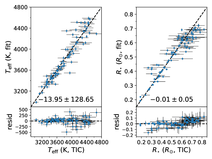
Figure 9: Comparison of $T_{\rm eff}$ and $R_{\star}$ as reported here compared to those from the TESS Input Catalogue. The median and standard deviation of each set of residuals is annotated.

6.5 Emission Features in TESS Candidates

While model limitations prevented us from taking full advantage of our spectra during fitting, our wide wavelength coverage allows us to look for spectral peculiarities. In the current study, these take the form of emission in the Hydrogen Balmer Series or Ca II H&K (both signs of stellar activity and youth), as well as absorption in the Li $6,708\,$$\text{\,}\mathrm{\SIUnitSymbolAngstrom}$ (another sign of youth). While none of our TESS planet hosts show detectable Lithium absorption, we report H$\alpha$ equivalent widths and $\log R^{\prime}_{\rm HK}$ in Table 3, calculated using the methodology of Žerjal et al. (2021). 53 stars in our sample have EWH$\alpha>-0.5\,$$\text{\,}\mathrm{\SIUnitSymbolAngstrom}$ (adopted as the limiting bound for activity, noting as well that this is strongly dependent on $T_{\rm eff}$ and thus somewhat approximate), and 35 have $\log R^{\prime}_{\rm HK}>-4.75$ (the lower bound for active stars used in Gray et al. 2006).

Of particular note are our two most active stars, the first of which is TOI 507 (TIC 348538431). TOI 507 appears substantially overluminous in Figure 1, and presents with strong emission across the Balmer Series and in Ca II H&K. Visual inspection of its spectrum, along with comparison to the cool dwarf standard HIP 103039 which is very similar in $T_{\rm eff}$, indicates that it is actually a double-lined spectroscopic binary. Transit depths appear similar for both primary and secondary eclipses, which points to the system being composed of roughly equal mass components. Taking a $\sim$0.75 mag offset into account due to binarity, TOI 507 still sits slightly above the main sequence, meaning that it remains a potentially young touchstone system amenable to characterisation as in e.g. Murphy et al. (2020). The mass, radius, $m_{\rm bol}$, and flux reported in Table 3 have been derived for a single component of this binary system, assuming equal mass and brightness.

The second star is TOI 142 (425934411) which is also overluminous and shows displays strong emission features. Interestingly, it appears to host a giant planet ($R_{P}=13.31\pm 1.39\,R_{\oplus}$) on a short period ($T\approx 0.85\,$day) - see Figure 10. While this is unusual for such a cool star, it is not unheard of, such as K2 32b which is a known short period super-Neptune orbiting a pre-main sequence star (David et al., 2016; Mann et al., 2016). Further characterisation of the system however, whilst scientifically interesting, is likely to be hampered by the faintness of the host star ($G$$\sim$$15.8$).

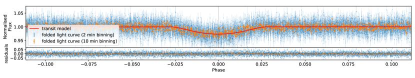
Figure 10: Phase folded light curve with best fitting transit model for TOI 142.01.

6.6 Planet Parameter Recovery

Table 19 collates literature parameters for previously characterised planets in our sample. These planets have typically had follow-up radial velocity observations which not only allows for planetary mass determination, but helps constrain their orbits when combined with the TESS light curves we use here (or additional time series photometric follow up). Figure 11 compares these results to our own for $R_{P}/R_{\star}$, $a/R_{\star}$, $i$, and $R_{P}$. We find our results consistent with the literature, aside from a few exceptions discussed below.

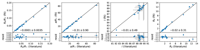
Figure 11: Comparison of $R_{P}/R_{\star}$, $a/R_{\star}$, $i$, and $R_{P}$ to literature results in Table 19. Our two largest literature planets, TOIs 129.01 and 551.01, are hot Jupiters in a grazing configuration which leaves their radii poorly constrained. As such, they have been left off for clarity, though our results are consistent within uncertainties. The median and standard deviation of each set of residuals is annotated and excludes these two planets.

6.6.1 LHS 3844 b

Vanderspek et al. (2019) reports a larger value of $Rp/R_{\star}$ for LHS 3844 b (TOI 136.01) than we do here, a difference we can attribute to our access to an extra sector of TESS data. While they also have ground based data, the extra TESS sector amounts to some 60 extra transits, which should give us improved precision.

6.6.2 HATS-48 A b, TOI 178 b/e, LHS 1140 c

Comparison with HATS-48 A b (TOI 1067.01) from Hartman et al. (2020) shows an inconsistent value of $R_{P}/R_{\star}$, indicating a difference in how we have modelled the light curves. While we have access to an additional sector of TESS data, the difference primarily appears to come from a) including RVs in their fit, and b) their use of an additional ‘dilution factor’ when fitting to account for nearby unresolved stars. Such nearby stars have the effect of diluting the transit and making the transit appear shallower than it would were only the flux from the host star observed. Our transit fits, by comparison, rely on the quality of the detrending and correction for crowding already done by the TESS team and provided in their PDCSAP fluxes.

Leleu et al. (2021) reports parameters for six planets orbiting TOI 178, of which only three were alerted on as TOIs. Our parameters are consistent for all but two of these, TOI 178 b (not alerted on) and TOI 178.03, both of which are relatively low SNR detections by TESS. Although our analysis includes an additional TESS sector of data, they employ higher precision data from CHEOPS to which we attribute the difference.

The analysis of LHS 1140 c (TOI 256.02) by Ment et al. (2019) results in a value of $R_{P}/R_{\star}$ discrepant with our own. While our analysis makes use of an additional sector of TESS data, we consider their results more reliable as they conducted a joint RV and transit photometry analysis, including additional ground based data alongside high precision Spitzer data.

6.6.3 WASP-43 b and HATS-6 b

We find a consistent $R_{P}/R_{\star}$ with Esposito et al. (2017) for WASP-43 b (TOI 656.01), though our value of $R_{P}$ is smaller. This difference is attributable to their larger and less precise stellar $T_{\rm eff}$, with which they obtain a smaller stellar radius - resulting in a smaller planetary radii. As discussed, we are confident with our $T_{\rm eff}$ and $R_{\star}$ recovery, and consider the difference the result of differing approaches to stellar parameter determination.

For HATS-6 b (TOI 468.01) we find our $R_{P}/R_{\star}$ and $T_{\rm eff}$ consistent, but a different value for $R_{P}$ as compared to Hartman et al. (2015). This difference again arises from a smaller literature value of $R_{\star}$. We consider our approach to radius determination using stellar fluxes more direct than the modelling based approach used here, especially given our access to precision Gaia parallaxes.

6.7 Candidate Planet Radii Distribution

We plot a histogram of our candidate planet radii in Figure 12, which shows the existence of the planet radius gap, first identified by Fulton et al. (2017), at $\sim$$1.65-2.0\,R_{\oplus}$ at a $\sim$$1\sigma$ level. As we remain limited by our small sample size, we do not perform any additional analysis and leave such investigations for future studies based on a larger sample of TESS planets.

Our results however do provide encouraging further evidence for the radius gap being present around planets orbiting low-mass stars. Its detection for the stellar mass range considered here is similar to the work of Cloutier & Menou (2020) who investigated a set of confirmed and candidate planets from Kepler and K2 orbiting stars with $T_{\rm eff}<4,700\,$K, with their sample being roughly a factor of ${\sim}4.5$ larger than our own. Separating their planets into bins of different stellar mass, they demonstrated that the bimodality in the radius distribution vanishes as stellar mass decreases, corresponding to the population of rocky planets beginning to dominate that of their more gas rich counterparts. They note, however, that a much larger sample of planets is required in order to properly distinguish between the various possible formation channels for the radius valley (e.g. photoevaporation, core-powered mass loss), particularly when further subdividing the sample by stellar mass. It is hoped that our results here can contribute to a larger future analysis combining Kepler, K2, and TESS planets, perhaps also looking into correlations with stellar activity using activity measures such as we provide.

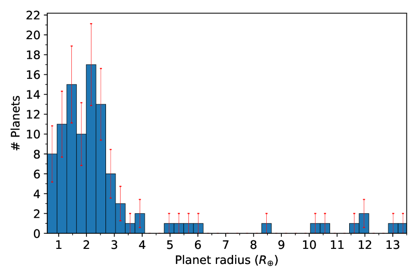
Figure 12: Histogram of candidate planet radii with $R_{P}<14\,R_{\oplus}$, with $0.35\,R_{\oplus}$ width bins and Poisson uncertainties. Note that we detect the exoplanet radius gap at approximately a $\sim$$1\sigma$ level, though remain limited by our small sample size.

7 Conclusions

In the work presented above, we have described our ANU 2.3 m/WiFeS observing program to characterise 92 southern TESS candidate planet hosts with $3,000\lesssim T_{\rm eff}\lesssim 4,500\,$K in order to precisely determine the radii of 100 transiting planets they host. In the process of doing so we investigated cool dwarf model atmosphere systematics, as well as developed a new photometric [Fe/H] calibration. The main conclusions from our work are as follows:

• Cool dwarf MARCS model atmospheres systematically overestimate flux in the optical relative to the well produced spectral regions $5585-6029\,$$\text{\,}\mathrm{\SIUnitSymbolAngstrom}$ and 6159-7000 $\text{\,}\mathrm{\SIUnitSymbolAngstrom}$, with agreement being worse the cooler the star or bluer the wavelength. We report a simple linear relation parameterising the offset as a function of the observed Gaia $(B_{P}-R_{P})$ colour, enabling the correction of synthetic Gaia $B_{P}$, and SkyMapper $g$ and $r$ magnitudes. We recommend that future work consider updated molecular line lists (McKemmish et al., 2019) and non-solar scaled chemical abundances (see Veyette et al. 2016).

• Using the same models, a general least squares fitting approach to medium resolution optical spectra and literature photometry is not sufficient to accurately recover [Fe/H] for cool dwarfs. We instead develop an updated photometric [Fe/H] calibration for cool dwarfs, built using a sample of 69 M and K dwarfs with FGK binary companions having reliable [Fe/H] measurements. By relating the position of these isolated main sequence KM stars in $M_{K_{S}}-(B_{P}-K_{S})$ space to the FGK companion, and thus system, [Fe/H], our relation can determine metallicity to a precision of $\pm 0.19\,$dex for stars with $1.51<(B_{P}-R_{P})<3.3$. This relation expands on the work of Bonfils et al. (2005), Johnson & Apps (2009), and Schlaufman & Laughlin (2010), and takes advantage of precision Gaia parallaxes (for precise distances) and kinematics (for binary identification) for the first time.

• We determine $T_{\rm eff}$ and $R_{\star}$ for our 92 TESS candidate planet hosts with a median precision of 0.8% and 1.7% respectively, as well as radial velocities to $\sim$$4.5\,$km s^-1. 42 of these targets did not previously have radial velocities from Gaia DR2, thus completing completing the kinematics for these stars.

• We report H$\alpha$ equivalent widths and Ca II H&K $\log R^{\prime}_{\rm HK}$ for our sample, both signs of activity and youth. None of our stars display detectable Lithium $6708\,$$\text{\,}\mathrm{\SIUnitSymbolAngstrom}$ absorption.

• We use our derived stellar parameters to fit the TESS light curves for our 100 planet candidates in order to determine $R_{P}$ with a median precision of 3.5%. Our planet properties are consistent with the 30 already confirmed by other studies. We additionally see evidence of the planet radius gap at a $\sim$$1\sigma$ level for our low-mass stellar sample, with the robustness of the detection only limited by the small sample size.

• We report the existence of two likely young systems based on stellar emission and location above the main sequence: TOI 507 (TIC 348538431) and TOI 142 (425934411). The former appears to be a near-equal mass, double-lined eclipsing binary with $T_{\rm eff}$$\approx$3300 K, potentially amenable to characterisation as a pre-main sequence benchmark system. TOI 142 on the other hand has a giant planet ($R_{P}=13.31\pm 1.39\,R_{\oplus}$) on a short period ($T\approx 0.85\,$day) orbit.

This is one of the largest uniform analyses of cool TESS candidate planet hosts to date, and the first cool dwarf photometric [Fe/H] calibration based on Gaia data. Given the major difficulties encountered using model atmospheres for [Fe/H] determination, we plan to conduct follow-up work investigating empirical or data driven approaches built upon our now large collection of cool dwarf standard spectra.

Data Availability

All fitted stellar and planetary results are available in the article and in its online supplementary material, and stellar spectra will be shared on reasonable request to the corresponding author. All other data used is publicly available.

Supporting Information

Supplementary data are available at MNRAS online.

Appendix A Observations

Table 7: Observing log for TESS candidate exoplanet host stars

TIC	UT Date	airmass	exp	RV	SNR
			(sec)	(km s-1)	(B)	(R)
219338557	19-08-25	1.1	120	36.00 $\pm$ 4.50	66	185
201248411	19-08-26	1.1	200	17.92 $\pm$ 4.50	52	142
262530407	19-08-26	1.1	200	8.71 $\pm$ 4.51	37	114
118327550	19-08-26	1.0	300	6.48 $\pm$ 4.53	23	75
410153553	19-08-26	1.3	600	-14.96 $\pm$ 4.55	14	63
62483237	19-08-26	1.0	150	6.17 $\pm$ 4.50	61	164
259377017	19-08-27	1.3	300	20.21 $\pm$ 4.53	26	84
200322593	19-08-27	1.4	600	12.61 $\pm$ 4.55	12	46
406941612	19-08-27	1.7	300	2.38 $\pm$ 4.52	24	80
193641523	19-08-27	1.7	300	26.62 $\pm$ 4.50	54	151
351601843	19-08-28	1.4	300	26.31 $\pm$ 4.51	21	71
234994474	19-08-28	1.1	300	24.29 $\pm$ 4.51	71	208
251848941	19-10-13	1.0	600	56.79 $\pm$ 4.50	72	199
259962054	19-10-14	1.2	300	-11.16 $\pm$ 4.54	6	27
101948569	19-10-14	1.0	120	22.63 $\pm$ 4.50	28	82
179985715	19-10-14	1.0	120	-12.54 $\pm$ 4.51	17	58
37749396	19-10-14	1.1	60	-9.28 $\pm$ 4.51	52	149
122613513	19-10-14	1.0	300	8.72 $\pm$ 4.50	54	145
229111835	19-10-14	1.1	300	13.15 $\pm$ 4.51	12	42
70899085	19-10-15	1.1	300	-12.74 $\pm$ 4.51	30	96
98796344	19-10-15	1.1	90	-10.03 $\pm$ 4.54	30	96
55488511	19-10-15	1.1	300	89.66 $\pm$ 4.51	18	63
271596225	19-10-15	1.4	300	-0.68 $\pm$ 4.52	15	53
44647437	19-10-16	1.0	300	14.43 $\pm$ 4.51	9	36
237914496	19-10-16	1.2	300	-6.74 $\pm$ 4.51	18	58
237920046	19-10-16	1.2	300	8.94 $\pm$ 4.51	12	43
201642601	19-10-17	1.3	900	-27.52 $\pm$ 4.51	16	57
158297421	19-10-17	1.2	900	-5.31 $\pm$ 4.50	14	49
261108236	19-10-17	1.5	600	4.02 $\pm$ 4.51	19	69
231702397	19-10-17	1.1	900	-76.33 $\pm$ 4.54	7	33
322063810	19-10-17	1.1	150	32.28 $\pm$ 4.51	47	137
220479565	19-10-17	1.1	600	30.73 $\pm$ 4.53	10	47
220459976	19-10-17	1.2	600	15.25 $\pm$ 4.51	20	73
192826603	19-10-17	1.1	1200	95.80 $\pm$ 4.52	7	38
44737596	19-10-17	1.1	1200	41.46 $\pm$ 4.52	6	36
38510224	19-10-17	1.2	300	29.91 $\pm$ 4.50	23	72
33831980	19-10-17	1.4	600	11.84 $\pm$ 4.51	25	85
219229644	19-10-17	1.1	300	48.73 $\pm$ 4.51	28	91
14165625	19-10-17	1.1	300	22.75 $\pm$ 4.50	27	86
32497972	19-10-17	1.0	300	3.57 $\pm$ 4.51	16	60
170849515	19-10-18	1.0	1800	4.86 $\pm$ 4.52	9	29
100608026	19-10-19	1.0	300	24.98 $\pm$ 4.51	29	97
144700903	19-10-19	1.4	700	-0.04 $\pm$ 4.51	12	53
12423815	19-11-16	1.0	2000	-11.69 $\pm$ 4.52	9	35
260708537	20-02-01	1.1	120	25.15 $\pm$ 4.53	32	102
35009898	20-02-01	1.2	600	-41.91 $\pm$ 4.53	14	52
151825527	20-02-01	1.0	450	-5.31 $\pm$ 4.52	23	80
150428135	20-02-01	1.2	360	-4.25 $\pm$ 4.53	29	92
260004324	20-02-01	1.1	180	41.76 $\pm$ 4.52	32	99
167600516	20-02-01	1.2	300	36.55 $\pm$ 4.51	45	136
219195044	20-02-01	1.1	450	117.69 $\pm$ 4.52	28	90
73649615	20-02-01	1.0	700	14.53 $\pm$ 4.52	12	50
165317334	20-02-01	1.0	150	4.98 $\pm$ 4.51	22	80
440887364	20-02-01	1.1	45	-25.52 $\pm$ 4.50	46	140
307210830	20-02-03	1.3	120	-5.17 $\pm$ 4.53	23	88
141608198	20-02-03	1.4	900	14.91 $\pm$ 4.54	8	44
33521996	20-02-03	1.0	900	41.68 $\pm$ 4.52	6	37
19025965	20-02-03	1.6	360	46.78 $\pm$ 4.50	17	73
27649847	20-02-03	1.4	720	-10.40 $\pm$ 4.53	8	44
413248763	20-02-03	1.0	45	-36.03 $\pm$ 4.53	22	80
296739893	20-02-03	1.1	300	8.47 $\pm$ 4.52	38	118
36734222	20-02-03	1.1	450	-8.65 $\pm$ 4.51	24	89
54962195	20-02-03	1.1	450	25.13 $\pm$ 4.52	7	44
158588995	20-02-03	1.0	720	7.25 $\pm$ 4.53	9	49

Table 8: continued

Observing log for TESS candidate exoplanet host stars TIC UT Date airmass exp RV SNR (sec) (km s^-1) (B) (R) 141527579 20-02-03 1.4 900 24.59 $\pm$ 4.52 20 75 149788158 20-02-03 1.2 360 24.03 $\pm$ 4.52 19 73 34068865 20-02-03 1.1 30 50.46 $\pm$ 4.52 30 99 36724087 20-02-03 1.1 360 -7.62 $\pm$ 4.53 14 60 359271092 20-02-03 1.2 20 37.39 $\pm$ 4.51 24 91 429358906 20-02-03 1.1 1200 -1.21 $\pm$ 4.54 6 43 374829238 20-02-03 1.2 600 15.29 $\pm$ 4.51 19 73 300710077 20-02-03 1.3 660 58.98 $\pm$ 4.53 12 60 362249359 20-02-03 1.2 180 14.78 $\pm$ 4.51 32 110 210873792 20-02-03 1.4 450 -75.36 $\pm$ 4.51 22 78 261257684 20-02-03 1.6 300 7.56 $\pm$ 4.51 25 91 280437559 20-02-03 1.3 180 -3.64 $\pm$ 4.50 25 91 370133522 20-09-11 1.3 180 -0.93 $\pm$ 4.53 20 70 12421862 20-09-11 1.0 180 19.29 $\pm$ 4.51 28 97 415969908 20-09-11 1.0 450 24.75 $\pm$ 4.52 20 71 92226327 20-09-11 1.1 450 -15.10 $\pm$ 4.55 9 44 348538431 20-09-11 2.0 900 -6.72 $\pm$ 4.56 15 56 254113311 20-09-12 1.0 180 -7.33 $\pm$ 4.50 39 115 29960110 20-09-12 1.0 360 26.52 $\pm$ 4.52 17 63 425934411 20-09-12 1.2 1200 -47.79 $\pm$ 4.53 11 52 153065527 20-09-12 1.0 450 17.50 $\pm$ 4.54 8 41 50618703 20-09-12 1.3 120 10.43 $\pm$ 4.50 36 111 77156829 20-09-12 1.0 300 9.06 $\pm$ 4.53 21 77 231728511 20-09-12 1.1 450 -5.94 $\pm$ 4.53 13 51 369327947 20-09-12 1.6 300 -13.78 $\pm$ 4.53 23 79 175532955 20-09-12 1.0 360 76.23 $\pm$ 4.50 25 79 141527965 20-09-13 1.4 450 37.43 $\pm$ 4.50 29 90 260417932 20-09-13 1.2 300 36.85 $\pm$ 4.50 42 116

Appendix B Stellar Standards

Table 9: Observing log for cool dwarf standards

Gaia DR2	UT Date	airmass	exp	RV	SNR
			(sec)	(km s-1)	(B)	(R)
19316224572460416	19-07-22	1.5	5	20.65 $\pm$ 4.50	108	251
2306965202564506752	19-07-22	1.0	200	19.60 $\pm$ 4.52	180	487
2603090003484152064	19-07-22	1.1	300	-4.68 $\pm$ 4.53	100	281
2683023811628007296	19-07-22	1.3	300	19.01 $\pm$ 4.51	159	462
2828928008202069376	19-07-22	1.5	200	-30.56 $\pm$ 4.51	158	458
5134635708766250752	19-07-22	1.1	300	8.56 $\pm$ 4.51	182	529
6553614253923452800	19-07-22	1.0	30	7.13 $\pm$ 4.51	117	335
6604147121141267712	19-07-22	1.0	30	8.13 $\pm$ 4.50	192	474
2552925644460225152	19-08-26	1.2	10	-14.82 $\pm$ 4.50	144	309
2627117287488522240	19-08-26	1.5	60	-18.10 $\pm$ 4.53	92	247
2653762573103102592	19-08-26	1.5	90	11.04 $\pm$ 4.51	94	271
2702655587447223168	19-08-26	1.6	300	-13.88 $\pm$ 4.51	74	219
2739689239311660672	19-08-26	1.2	90	-79.67 $\pm$ 4.52	73	213
4282578724832056576	19-08-26	1.7	120	9.19 $\pm$ 4.51	82	234
4293318823182081408	19-08-26	1.7	100	30.79 $\pm$ 4.52	85	228
6412595290592307840	19-08-26	1.1	6	-42.60 $\pm$ 4.50	296	711
6562924609150908416	19-08-26	1.1	60	7.74 $\pm$ 4.52	180	492
2611163717366876544	19-08-27	1.2	60	-11.00 $\pm$ 4.51	45	139
2815543034682035840	19-08-27	1.6	90	-7.36 $\pm$ 4.51	44	136
3209938366665770752	19-08-27	2.6	30	2.25 $\pm$ 4.51	66	209
114207651462714880	19-10-12	1.9	300	26.03 $\pm$ 4.53	114	346
2515037264041041536	19-10-12	1.2	120	-10.79 $\pm$ 4.52	110	309
2560771312759450496	19-10-12	1.2	180	-31.93 $\pm$ 4.52	77	227
301785537751949824	19-10-12	2.0	300	-9.94 $\pm$ 4.51	65	211
87921523897823872	19-10-12	1.7	300	-4.49 $\pm$ 4.52	65	197
145421309108301184	19-10-14	1.7	60	-35.17 $\pm$ 4.51	93	282
3210731015767419520	19-10-14	1.2	30	-55.79 $\pm$ 4.50	109	278
3339921875389105152	19-10-14	1.4	120	20.00 $\pm$ 4.51	108	318
3359074685047632640	19-10-14	1.8	200	-60.17 $\pm$ 4.51	91	282
3409711211681795584	19-10-14	1.6	180	23.09 $\pm$ 4.52	78	233
1736838805468812160	19-10-15	1.4	30	-70.90 $\pm$ 4.50	58	162
3057712188691831936	19-10-15	1.2	90	-20.08 $\pm$ 4.51	92	274
4075141768785646848	19-10-15	1.5	60	-9.52 $\pm$ 4.55	32	110
4971496564348094336	19-10-15	1.0	90	43.73 $\pm$ 4.52	52	148
5006921282807193856	19-10-15	1.0	150	40.49 $\pm$ 4.51	61	179
2910909931633597312	19-10-17	1.0	144	53.69 $\pm$ 4.52	44	125
2979590513145784192	19-10-17	1.0	144	-15.39 $\pm$ 4.52	43	131
3101920046552857728	19-10-17	1.2	90	-11.34 $\pm$ 4.52	65	184
3117120863523946368	19-10-17	1.2	90	11.51 $\pm$ 4.55	25	91
3136952686035250688	19-10-17	1.4	90	19.87 $\pm$ 4.56	25	87
3184351876391975808	19-10-17	1.1	90	-10.63 $\pm$ 4.52	44	130
3316364602541746048	19-10-17	1.2	144	24.40 $\pm$ 4.54	31	104
5951824121022278144	19-10-17	1.5	108	-8.80 $\pm$ 4.53	75	223
3057712223051571200	20-02-01	1.1	12	-13.82 $\pm$ 4.50	99	231
4364527594192166400	20-02-01	2.1	15	36.77 $\pm$ 4.51	65	195
5378886891122066560	20-02-01	1.0	15	14.90 $\pm$ 4.50	81	206
6143175840404555008	20-02-01	1.0	24	-4.07 $\pm$ 4.50	35	101
6223456372670070656	20-02-01	1.1	90	18.75 $\pm$ 4.50	79	202
6288325222245417856	20-02-01	1.0	15	-36.71 $\pm$ 4.50	63	184
1244644727396803584	20-02-03	1.6	60	24.60 $\pm$ 4.51	46	152
3089711447388931584	20-02-03	1.2	60	65.99 $\pm$ 4.52	44	138
3195919322830293760	20-02-03	1.1	144	-45.15 $\pm$ 4.55	41	120
3256334497479041024	20-02-03	1.2	15	13.50 $\pm$ 4.50	55	152
3520548825260557312	20-02-03	1.0	60	112.47 $\pm$ 4.51	64	158
3550084490721711872	20-02-03	1.1	90	30.33 $\pm$ 4.50	51	143
3630092241022731136	20-02-03	1.1	36	-15.90 $\pm$ 4.50	51	144
3661492609484469504	20-02-03	1.2	60	-37.17 $\pm$ 4.50	75	210
3689602277083844480	20-02-03	1.2	72	8.91 $\pm$ 4.51	105	321
3738099879558957952	20-02-03	1.4	72	18.94 $\pm$ 4.51	79	240
3741297293732404352	20-02-03	1.5	45	19.02 $\pm$ 4.52	80	235
3767878708888402816	20-02-03	1.2	90	26.64 $\pm$ 4.51	53	163
3796072592206250624	20-02-03	1.2	120	-34.21 $\pm$ 4.54	21	90
3828238392559860992	20-02-03	1.3	120	10.18 $\pm$ 4.52	92	268
3855208897392952192	20-02-03	1.3	120	6.61 $\pm$ 4.52	70	211

Table 10: continued

Observing log for cool dwarf standards Gaia DR2 UT Date airmass exp RV SNR (sec) (km s^-1) (B) (R) 3902785109124370432 20-02-03 1.4 300 20.95 $\pm$ 4.51 106 322 4017860992519744384 20-02-03 1.9 120 4.28 $\pm$ 4.53 33 118 4330690742322011520 20-02-03 1.4 120 -25.48 $\pm$ 4.53 62 195 4364480521350598144 20-02-03 1.8 60 31.88 $\pm$ 4.52 39 130 5170039502144332800 20-02-03 1.2 15 -1.55 $\pm$ 4.50 58 164 5266270443442455040 20-02-03 1.3 90 18.99 $\pm$ 4.50 70 183 614543647497149056 20-02-03 1.6 90 12.23 $\pm$ 4.52 36 118 6232511606838403968 20-02-03 1.2 7 27.29 $\pm$ 4.50 130 330 6324325225803432320 20-02-03 1.2 144 -1.32 $\pm$ 4.54 38 122 116037376250217984 20-09-11 1.9 500 25.26 $\pm$ 4.53 28 99 1750765357185849856 20-09-11 1.5 500 -25.65 $\pm$ 4.54 25 96 18565464288396416 20-09-11 1.3 240 20.98 $\pm$ 4.53 36 112 2029432043779954432 20-09-11 2.4 600 -48.01 $\pm$ 4.54 11 52 2316867885320845696 20-09-11 1.0 150 16.65 $\pm$ 4.52 35 109 2358524597030794112 20-09-11 1.1 240 18.71 $\pm$ 4.56 26 98 2435125446129139712 20-09-11 1.1 450 -30.75 $\pm$ 4.53 27 94 2533723464155234176 20-09-11 1.3 150 13.99 $\pm$ 4.51 46 144 2595284016771502080 20-09-11 1.0 600 -14.03 $\pm$ 4.55 23 86 2640434056928150400 20-09-11 1.2 500 -41.88 $\pm$ 4.56 9 64 2817999068780218368 20-09-11 1.6 240 -7.29 $\pm$ 4.54 32 103 4145870293808914688 20-09-11 1.1 920 -46.19 $\pm$ 4.55 21 66 4177731838628465408 20-09-11 1.2 36 23.09 $\pm$ 4.52 43 132 4187836934609063552 20-09-11 1.1 1500 -58.36 $\pm$ 4.54 31 102 4303294035005560704 20-09-11 1.5 450 -0.34 $\pm$ 4.53 37 117 4339465360508118912 20-09-11 1.2 240 12.31 $\pm$ 4.54 34 111 4365609170043180416 20-09-11 1.2 360 -11.77 $\pm$ 4.55 31 105 4375233191015944192 20-09-11 1.3 15 -22.90 $\pm$ 4.51 65 197 4389844948935164544 20-09-11 1.3 45 -14.11 $\pm$ 4.51 47 148 4472832130942575872 20-09-11 1.3 30 -109.09 $\pm$ 4.56 29 106 4498055584805914752 20-09-11 1.7 920 -28.75 $\pm$ 4.54 32 107 4550763526539955712 20-09-11 1.7 45 -11.93 $\pm$ 4.51 38 123 4572835535272064768 20-09-11 2.2 60 2.41 $\pm$ 4.51 41 136 4584638930036248192 20-09-11 2.5 600 -2.63 $\pm$ 4.52 31 108 5042734468172061440 20-09-11 1.1 240 -41.49 $\pm$ 4.52 49 149 5853498713160606720 20-09-11 1.4 60 -26.88 $\pm$ 4.56 49 187 6245870673116518784 20-09-11 1.2 180 -2.02 $\pm$ 4.53 38 113 6322070093095493504 20-09-11 1.5 120 -9.91 $\pm$ 4.53 42 133 6882963066420161664 20-09-11 1.2 150 6.16 $\pm$ 4.54 27 96 6885776098199761024 20-09-11 1.2 150 -66.40 $\pm$ 4.52 41 131 6890353330746858368 20-09-11 1.2 240 27.46 $\pm$ 4.53 42 124 76868614540049408 20-09-11 1.5 240 -34.31 $\pm$ 4.56 21 83 102162639019033600 20-09-12 1.9 600 -10.88 $\pm$ 4.54 21 79 1784473016438653056 20-09-12 1.6 60 -27.82 $\pm$ 4.53 32 106 1809359465717142656 20-09-12 1.6 500 -51.83 $\pm$ 4.54 20 64 1810616448010879488 20-09-12 1.6 450 -62.47 $\pm$ 4.54 27 98 1814070838668707840 20-09-12 1.8 90 5.78 $\pm$ 4.51 40 129 1838855376946302720 20-09-12 1.9 294 -31.81 $\pm$ 4.53 30 104 2507016253701863040 20-09-12 1.2 450 21.18 $\pm$ 4.54 26 89 2976850598890038784 20-09-12 1.2 240 9.31 $\pm$ 4.53 28 95 3187115498866675456 20-09-12 1.4 240 32.96 $\pm$ 4.55 23 85 3219851121121855872 20-09-12 1.3 500 31.72 $\pm$ 4.52 38 120 3239548631415741440 20-09-12 1.6 360 40.94 $\pm$ 4.52 35 111 3288082758293022848 20-09-12 1.7 240 -15.01 $\pm$ 4.53 27 88 35398295820372864 20-09-12 1.6 600 -37.31 $\pm$ 4.54 20 74 4295619138933719808 20-09-12 1.4 600 19.28 $\pm$ 4.54 30 96 4393265392167891712 20-09-12 1.4 600 11.05 $\pm$ 4.54 22 76 4508377078422114944 20-09-12 1.5 360 -48.72 $\pm$ 4.54 26 82 4512525016089353472 20-09-12 1.7 500 11.51 $\pm$ 4.55 31 108 4519789081415296128 20-09-12 1.9 150 30.19 $\pm$ 4.53 40 134 4519789321933481856 20-09-12 1.9 150 32.15 $\pm$ 4.53 40 135 4535928365908540416 20-09-12 2.2 240 22.56 $\pm$ 4.54 17 56 5077642283022422656 20-09-12 1.0 90 31.72 $\pm$ 4.51 42 130 2467732906559754496 20-09-13 1.1 500 -5.83 $\pm$ 4.56 21 80 2549050931124387456 20-09-13 1.2 600 -5.17 $\pm$ 4.53 31 100

Table 11: continued

Observing log for cool dwarf standards Gaia DR2 UT Date airmass exp RV SNR (sec) (km s^-1) (B) (R) 2848646203058386560 20-09-13 1.7 450 -48.92 $\pm$ 4.53 37 116 2868199402451064064 20-09-13 2.2 600 -15.06 $\pm$ 4.56 21 85 2911981886751531648 20-09-13 1.1 240 4.93 $\pm$ 4.53 34 106 3011648664439643520 20-09-13 1.1 120 21.03 $\pm$ 4.50 46 127 3131777319158582272 20-09-13 1.4 300 -6.02 $\pm$ 4.52 28 97 3266980243936341248 20-09-13 1.2 600 82.84 $\pm$ 4.52 28 93 4706630501049679744 20-09-13 1.4 60 39.09 $\pm$ 4.50 96 243 4871271406553197184 20-09-13 1.0 90 26.97 $\pm$ 4.50 53 140 5142772953804963456 20-09-13 1.1 600 -2.48 $\pm$ 4.53 38 119 6391176735363140480 20-09-13 1.4 30 4.49 $\pm$ 4.50 69 192

Table 12: Final results for cool dwarf standards

Gaia DR2	$T_{\rm eff}$	$\log g$	[Fe/H]	$M$	$R_{\star}$	$m_{\rm bol}$	$f_{\rm bol}$
	(K)			($M_{\odot}$)	($R_{\odot}$)		(10${}^{-12}\,$ergs s-1 cm -2)
5853498713160606720	2885 $\pm$ 30	5.14 $\pm$ 0.02	-	0.124 $\pm$ 0.003	0.156 $\pm$ 0.003	7.36 $\pm$ 0.01	28793.2 $\pm$ 291.5
2640434056928150400	2927 $\pm$ 30	5.20 $\pm$ 0.02	-	0.120 $\pm$ 0.003	0.144 $\pm$ 0.003	11.19 $\pm$ 0.01	851.2 $\pm$ 8.9
2595284016771502080	3006 $\pm$ 30	5.03 $\pm$ 0.02	-	0.176 $\pm$ 0.004	0.212 $\pm$ 0.004	10.25 $\pm$ 0.01	2020.5 $\pm$ 21.1
2467732906559754496	3022 $\pm$ 30	5.10 $\pm$ 0.02	-	0.145 $\pm$ 0.004	0.178 $\pm$ 0.004	11.43 $\pm$ 0.01	680.0 $\pm$ 7.0
4393265392167891712	3035 $\pm$ 30	5.03 $\pm$ 0.02	-	0.181 $\pm$ 0.004	0.214 $\pm$ 0.004	11.71 $\pm$ 0.01	524.2 $\pm$ 5.4
4145870293808914688	3061 $\pm$ 30	5.08 $\pm$ 0.02	-	0.153 $\pm$ 0.004	0.187 $\pm$ 0.004	10.65 $\pm$ 0.01	1398.5 $\pm$ 14.2
2358524597030794112	3062 $\pm$ 30	5.13 $\pm$ 0.02	-0.29	0.137 $\pm$ 0.003	0.167 $\pm$ 0.003	9.24 $\pm$ 0.01	5113.3 $\pm$ 52.0
1810616448010879488	3064 $\pm$ 30	4.99 $\pm$ 0.02	-	0.190 $\pm$ 0.005	0.231 $\pm$ 0.005	10.58 $\pm$ 0.01	1488.6 $\pm$ 14.8
76868614540049408	3069 $\pm$ 30	5.09 $\pm$ 0.02	-0.17	0.148 $\pm$ 0.003	0.182 $\pm$ 0.004	9.45 $\pm$ 0.01	4221.2 $\pm$ 42.1
2868199402451064064	3088 $\pm$ 30	5.06 $\pm$ 0.02	-0.15	0.156 $\pm$ 0.004	0.192 $\pm$ 0.004	11.58 $\pm$ 0.01	591.2 $\pm$ 5.9
3117120863523946368	3094 $\pm$ 30	4.91 $\pm$ 0.02	-	0.236 $\pm$ 0.006	0.281 $\pm$ 0.006	8.29 $\pm$ 0.01	12313.6 $\pm$ 123.2
1750765357185849856	3121 $\pm$ 30	5.04 $\pm$ 0.02	-	0.183 $\pm$ 0.004	0.215 $\pm$ 0.004	11.30 $\pm$ 0.01	765.6 $\pm$ 7.7
2029432043779954432	3128 $\pm$ 30	4.98 $\pm$ 0.02	0.23	0.206 $\pm$ 0.005	0.242 $\pm$ 0.005	11.51 $\pm$ 0.01	632.4 $\pm$ 6.3
3796072592206250624	3136 $\pm$ 30	5.06 $\pm$ 0.02	-0.08	0.176 $\pm$ 0.004	0.206 $\pm$ 0.004	8.47 $\pm$ 0.01	10415.1 $\pm$ 105.8
2549050931124387456	3139 $\pm$ 30	4.72 $\pm$ 0.02	-	0.384 $\pm$ 0.009	0.445 $\pm$ 0.009	12.05 $\pm$ 0.01	385.1 $\pm$ 3.9
3187115498866675456	3142 $\pm$ 30	5.08 $\pm$ 0.02	-0.14	0.171 $\pm$ 0.004	0.198 $\pm$ 0.004	9.56 $\pm$ 0.01	3810.3 $\pm$ 38.7
3195919322830293760	3160 $\pm$ 30	4.94 $\pm$ 0.02	-	0.231 $\pm$ 0.006	0.269 $\pm$ 0.005	8.72 $\pm$ 0.01	8276.6 $\pm$ 84.2
4512525016089353472	3167 $\pm$ 30	4.98 $\pm$ 0.02	-	0.207 $\pm$ 0.005	0.244 $\pm$ 0.005	11.16 $\pm$ 0.01	869.9 $\pm$ 8.7
102162639019033600	3169 $\pm$ 30	4.98 $\pm$ 0.02	0.05	0.212 $\pm$ 0.005	0.246 $\pm$ 0.005	10.39 $\pm$ 0.01	1773.4 $\pm$ 17.7
6882963066420161664	3173 $\pm$ 30	4.97 $\pm$ 0.02	-	0.232 $\pm$ 0.006	0.261 $\pm$ 0.005	9.01 $\pm$ 0.01	6339.3 $\pm$ 64.0
4472832130942575872	3188 $\pm$ 30	5.06 $\pm$ 0.02	-0.51	0.160 $\pm$ 0.004	0.195 $\pm$ 0.004	7.19 $\pm$ 0.01	33821.5 $\pm$ 338.4
4535928365908540416	3201 $\pm$ 30	4.83 $\pm$ 0.02	0.65	0.342 $\pm$ 0.008	0.370 $\pm$ 0.007	9.45 $\pm$ 0.01	4204.3 $\pm$ 42.0
4075141768785646848	3204 $\pm$ 30	5.06 $\pm$ 0.02	-0.32	0.177 $\pm$ 0.004	0.207 $\pm$ 0.004	8.10 $\pm$ 0.01	14680.7 $\pm$ 146.2
3316364602541746048	3206 $\pm$ 30	4.97 $\pm$ 0.02	0.05	0.231 $\pm$ 0.006	0.262 $\pm$ 0.005	8.79 $\pm$ 0.01	7711.6 $\pm$ 76.7
4187836934609063552	3208 $\pm$ 30	4.98 $\pm$ 0.02	-0.01	0.230 $\pm$ 0.006	0.258 $\pm$ 0.005	11.48 $\pm$ 0.01	649.8 $\pm$ 6.5
1809359465717142656	3221 $\pm$ 30	4.92 $\pm$ 0.02	-	0.244 $\pm$ 0.006	0.282 $\pm$ 0.005	11.56 $\pm$ 0.01	605.2 $\pm$ 6.0
4365609170043180416	3224 $\pm$ 30	4.98 $\pm$ 0.02	-0.02	0.235 $\pm$ 0.006	0.260 $\pm$ 0.005	9.90 $\pm$ 0.01	2796.5 $\pm$ 28.1
2507016253701863040	3227 $\pm$ 30	4.97 $\pm$ 0.02	0.21	0.256 $\pm$ 0.006	0.275 $\pm$ 0.005	10.99 $\pm$ 0.01	1017.2 $\pm$ 10.3
18565464288396416	3234 $\pm$ 30	4.92 $\pm$ 0.02	0.02	0.252 $\pm$ 0.006	0.288 $\pm$ 0.005	9.26 $\pm$ 0.01	5022.8 $\pm$ 50.2
3136952686035250688	3241 $\pm$ 30	4.88 $\pm$ 0.02	0.44	0.315 $\pm$ 0.007	0.336 $\pm$ 0.006	8.51 $\pm$ 0.01	10006.1 $\pm$ 101.8
4339465360508118912	3247 $\pm$ 30	5.01 $\pm$ 0.02	-	0.209 $\pm$ 0.005	0.237 $\pm$ 0.004	9.44 $\pm$ 0.01	4269.1 $\pm$ 42.5
2848646203058386560	3250 $\pm$ 30	4.78 $\pm$ 0.02	-	0.373 $\pm$ 0.009	0.410 $\pm$ 0.008	10.73 $\pm$ 0.01	1293.0 $\pm$ 12.9
3288082758293022848	3250 $\pm$ 30	4.81 $\pm$ 0.02	-	0.366 $\pm$ 0.009	0.393 $\pm$ 0.007	9.73 $\pm$ 0.01	3258.4 $\pm$ 32.9
4508377078422114944	3265 $\pm$ 30	4.89 $\pm$ 0.02	0.14	0.294 $\pm$ 0.007	0.322 $\pm$ 0.006	10.09 $\pm$ 0.01	2345.5 $\pm$ 23.3
4303294035005560704	3277 $\pm$ 30	4.82 $\pm$ 0.02	-	0.354 $\pm$ 0.009	0.383 $\pm$ 0.007	10.75 $\pm$ 0.01	1279.4 $\pm$ 12.7
2435125446129139712	3278 $\pm$ 30	4.95 $\pm$ 0.02	0.32	0.303 $\pm$ 0.008	0.305 $\pm$ 0.006	10.93 $\pm$ 0.01	1081.2 $\pm$ 11.1
116037376250217984	3282 $\pm$ 30	4.90 $\pm$ 0.02	0.19	0.304 $\pm$ 0.007	0.324 $\pm$ 0.006	11.41 $\pm$ 0.01	692.3 $\pm$ 6.9
6324325225803432320	3283 $\pm$ 30	4.96 $\pm$ 0.02	0.32	0.294 $\pm$ 0.008	0.299 $\pm$ 0.006	8.80 $\pm$ 0.01	7681.5 $\pm$ 78.9
4295619138933719808	3299 $\pm$ 30	5.01 $\pm$ 0.02	-0.37	0.220 $\pm$ 0.005	0.242 $\pm$ 0.004	10.39 $\pm$ 0.01	1781.8 $\pm$ 17.9
1784473016438653056	3303 $\pm$ 30	4.76 $\pm$ 0.02	-	0.395 $\pm$ 0.009	0.433 $\pm$ 0.008	8.14 $\pm$ 0.01	14033.5 $\pm$ 139.9
4330690742322011520	3309 $\pm$ 30	4.91 $\pm$ 0.02	0.07	0.302 $\pm$ 0.008	0.321 $\pm$ 0.006	7.80 $\pm$ 0.01	19231.6 $\pm$ 191.5
2603090003484152064	3326 $\pm$ 30	4.89 $\pm$ 0.02	0.29	0.338 $\pm$ 0.008	0.347 $\pm$ 0.006	7.79 $\pm$ 0.01	19393.6 $\pm$ 194.0
35398295820372864	3330 $\pm$ 30	4.81 $\pm$ 0.02	-	0.370 $\pm$ 0.010	0.396 $\pm$ 0.009	10.57 $\pm$ 0.01	1508.8 $\pm$ 15.0
2976850598890038784	3337 $\pm$ 30	4.96 $\pm$ 0.02	-	0.274 $\pm$ 0.007	0.287 $\pm$ 0.005	9.66 $\pm$ 0.01	3465.4 $\pm$ 34.6
2817999068780218368	3344 $\pm$ 30	4.83 $\pm$ 0.02	0.39	0.381 $\pm$ 0.009	0.394 $\pm$ 0.007	9.26 $\pm$ 0.01	5021.5 $\pm$ 50.0
6322070093095493504	3360 $\pm$ 30	4.90 $\pm$ 0.02	-0.10	0.311 $\pm$ 0.008	0.327 $\pm$ 0.006	8.52 $\pm$ 0.01	9900.6 $\pm$ 98.6
6245870673116518784	3360 $\pm$ 30	4.69 $\pm$ 0.02	-	0.481 $\pm$ 0.011	0.515 $\pm$ 0.009	9.35 $\pm$ 0.01	4619.8 $\pm$ 46.8
2911981886751531648	3362 $\pm$ 30	4.92 $\pm$ 0.02	-0.13	0.305 $\pm$ 0.007	0.316 $\pm$ 0.006	9.88 $\pm$ 0.01	2831.9 $\pm$ 28.5
4498055584805914752	3385 $\pm$ 30	4.97 $\pm$ 0.02	-0.36	0.259 $\pm$ 0.006	0.276 $\pm$ 0.005	11.28 $\pm$ 0.01	785.0 $\pm$ 7.8
114207651462714880	3403 $\pm$ 30	4.84 $\pm$ 0.02	-0.08	0.357 $\pm$ 0.009	0.374 $\pm$ 0.007	8.60 $\pm$ 0.01	9191.7 $\pm$ 91.6
5951824121022278144	3435 $\pm$ 30	4.88 $\pm$ 0.02	-0.13	0.353 $\pm$ 0.008	0.359 $\pm$ 0.006	7.52 $\pm$ 0.01	25039.0 $\pm$ 249.3
3219851121121855872	3456 $\pm$ 30	4.69 $\pm$ 0.02	-	0.498 $\pm$ 0.012	0.524 $\pm$ 0.009	11.50 $\pm$ 0.01	636.8 $\pm$ 6.4
4017860992519744384	3459 $\pm$ 30	4.79 $\pm$ 0.02	0.05	0.423 $\pm$ 0.010	0.434 $\pm$ 0.008	8.73 $\pm$ 0.01	8170.7 $\pm$ 81.3
5142772953804963456	3483 $\pm$ 30	4.89 $\pm$ 0.02	-	0.352 $\pm$ 0.008	0.354 $\pm$ 0.006	12.06 $\pm$ 0.01	379.6 $\pm$ 3.8
1838855376946302720	3484 $\pm$ 30	4.93 $\pm$ 0.02	-	0.311 $\pm$ 0.008	0.315 $\pm$ 0.006	10.24 $\pm$ 0.01	2033.8 $\pm$ 20.3
2560771312759450496	3497 $\pm$ 30	4.84 $\pm$ 0.02	-0.13	0.403 $\pm$ 0.010	0.402 $\pm$ 0.007	9.17 $\pm$ 0.01	5445.7 $\pm$ 54.4
2627117287488522240	3505 $\pm$ 30	4.77 $\pm$ 0.02	0.29	0.465 $\pm$ 0.011	0.463 $\pm$ 0.008	8.31 $\pm$ 0.01	12075.4 $\pm$ 120.5
6890353330746858368	3511 $\pm$ 30	4.76 $\pm$ 0.02	0.17	0.468 $\pm$ 0.011	0.470 $\pm$ 0.008	9.58 $\pm$ 0.01	3738.4 $\pm$ 37.5
4584638930036248192	3516 $\pm$ 30	4.76 $\pm$ 0.02	-0.05	0.448 $\pm$ 0.011	0.460 $\pm$ 0.008	10.85 $\pm$ 0.01	1166.3 $\pm$ 11.6
2979590513145784192	3522 $\pm$ 30	4.83 $\pm$ 0.02	-0.19	0.409 $\pm$ 0.010	0.407 $\pm$ 0.007	9.23 $\pm$ 0.01	5167.2 $\pm$ 51.5
3239548631415741440	3530 $\pm$ 30	4.48 $\pm$ 0.02	-	0.624 $\pm$ 0.015	0.747 $\pm$ 0.013	10.28 $\pm$ 0.01	1955.6 $\pm$ 19.5
3101920046552857728	3533 $\pm$ 30	4.79 $\pm$ 0.02	-0.07	0.441 $\pm$ 0.012	0.445 $\pm$ 0.008	8.35 $\pm$ 0.01	11628.5 $\pm$ 115.7
3089711447388931584	3534 $\pm$ 30	4.79 $\pm$ 0.02	-0.09	0.442 $\pm$ 0.011	0.444 $\pm$ 0.008	8.40 $\pm$ 0.01	11122.0 $\pm$ 110.7
3855208897392952192	3540 $\pm$ 30	4.81 $\pm$ 0.02	-0.11	0.431 $\pm$ 0.010	0.429 $\pm$ 0.007	7.95 $\pm$ 0.01	16866.3 $\pm$ 167.9

Table 13: continued

Final results for cool dwarf standards Gaia DR2 $T_{\rm eff}$ $\log g$ [Fe/H] $M$ $R_{\star}$ $m_{\rm bol}$ $f_{\rm bol}$ (K) ($M_{\odot}$) ($R_{\odot}$) (10${}^{-12}\,$ergs s^-1 cm ^-2) 4519789081415296128 3541 $\pm$ 30 4.94 $\pm$ 0.02 - 0.319 $\pm$ 0.008 0.319 $\pm$ 0.005 9.08 $\pm$ 0.01 5906.7 $\pm$ 58.9 4519789321933481856 3543 $\pm$ 30 4.94 $\pm$ 0.02 - 0.318 $\pm$ 0.008 0.317 $\pm$ 0.005 9.09 $\pm$ 0.01 5856.8 $\pm$ 58.4 3131777319158582272 3545 $\pm$ 30 4.65 $\pm$ 0.02 - 0.528 $\pm$ 0.013 0.566 $\pm$ 0.010 10.46 $\pm$ 0.01 1659.9 $\pm$ 16.5 3184351876391975808 3555 $\pm$ 30 4.75 $\pm$ 0.02 - 0.470 $\pm$ 0.011 0.478 $\pm$ 0.008 8.70 $\pm$ 0.01 8389.8 $\pm$ 83.5 4293318823182081408 3555 $\pm$ 30 4.76 $\pm$ 0.02 0.07 0.474 $\pm$ 0.011 0.476 $\pm$ 0.008 7.32 $\pm$ 0.01 29932.3 $\pm$ 298.2 3409711211681795584 3560 $\pm$ 30 4.73 $\pm$ 0.02 0.06 0.489 $\pm$ 0.012 0.500 $\pm$ 0.009 8.24 $\pm$ 0.01 12905.3 $\pm$ 128.4 2910909931633597312 3582 $\pm$ 30 4.71 $\pm$ 0.02 0.26 0.517 $\pm$ 0.012 0.527 $\pm$ 0.009 8.95 $\pm$ 0.01 6698.1 $\pm$ 66.7 614543647497149056 3583 $\pm$ 30 4.75 $\pm$ 0.02 -0.07 0.474 $\pm$ 0.011 0.478 $\pm$ 0.008 8.73 $\pm$ 0.01 8157.1 $\pm$ 81.2 87921523897823872 3601 $\pm$ 30 4.72 $\pm$ 0.02 0.10 0.511 $\pm$ 0.012 0.518 $\pm$ 0.009 8.97 $\pm$ 0.01 6591.2 $\pm$ 65.6 6885776098199761024 3611 $\pm$ 30 4.91 $\pm$ 0.02 -0.56 0.355 $\pm$ 0.009 0.345 $\pm$ 0.006 9.46 $\pm$ 0.01 4186.0 $\pm$ 41.8 4364480521350598144 3615 $\pm$ 30 4.77 $\pm$ 0.02 -0.21 0.464 $\pm$ 0.011 0.467 $\pm$ 0.008 8.53 $\pm$ 0.01 9818.2 $\pm$ 97.8 6562924609150908416 3615 $\pm$ 30 4.81 $\pm$ 0.02 -0.22 0.440 $\pm$ 0.010 0.434 $\pm$ 0.007 7.07 $\pm$ 0.01 37591.6 $\pm$ 374.6 4971496564348094336 3618 $\pm$ 30 4.71 $\pm$ 0.02 0.04 0.516 $\pm$ 0.012 0.526 $\pm$ 0.009 8.71 $\pm$ 0.01 8361.5 $\pm$ 83.2 2316867885320845696 3622 $\pm$ 30 4.71 $\pm$ 0.02 0.16 0.525 $\pm$ 0.012 0.530 $\pm$ 0.009 9.43 $\pm$ 0.01 4283.9 $\pm$ 42.6 3828238392559860992 3627 $\pm$ 30 4.72 $\pm$ 0.02 0.03 0.512 $\pm$ 0.012 0.518 $\pm$ 0.009 7.63 $\pm$ 0.01 22534.9 $\pm$ 224.3 2515037264041041536 3635 $\pm$ 30 4.79 $\pm$ 0.02 -0.33 0.449 $\pm$ 0.011 0.449 $\pm$ 0.008 8.60 $\pm$ 0.01 9214.0 $\pm$ 92.0 4550763526539955712 3638 $\pm$ 30 4.81 $\pm$ 0.02 -0.32 0.442 $\pm$ 0.010 0.436 $\pm$ 0.007 8.12 $\pm$ 0.01 14421.3 $\pm$ 143.6 3767878708888402816 3647 $\pm$ 30 4.70 $\pm$ 0.02 -0.01 0.526 $\pm$ 0.013 0.538 $\pm$ 0.009 8.63 $\pm$ 0.01 8991.2 $\pm$ 89.5 4177731838628465408 3649 $\pm$ 30 4.79 $\pm$ 0.02 -0.22 0.466 $\pm$ 0.011 0.456 $\pm$ 0.008 7.89 $\pm$ 0.01 17811.0 $\pm$ 177.3 6553614253923452800 3656 $\pm$ 30 4.74 $\pm$ 0.04 -0.35 0.463 $\pm$ 0.034 0.479 $\pm$ 0.008 5.91 $\pm$ 0.01 109647.8 $\pm$ 1093.2 3741297293732404352 3657 $\pm$ 30 4.75 $\pm$ 0.02 -0.19 0.487 $\pm$ 0.011 0.486 $\pm$ 0.008 6.97 $\pm$ 0.01 41290.1 $\pm$ 411.5 5042734468172061440 3660 $\pm$ 30 4.77 $\pm$ 0.02 - 0.484 $\pm$ 0.011 0.476 $\pm$ 0.008 9.68 $\pm$ 0.01 3399.1 $\pm$ 33.9 2739689239311660672 3673 $\pm$ 30 4.85 $\pm$ 0.02 -0.44 0.413 $\pm$ 0.010 0.399 $\pm$ 0.007 7.56 $\pm$ 0.01 23962.9 $\pm$ 238.6 4572835535272064768 3680 $\pm$ 30 4.72 $\pm$ 0.02 -0.09 0.518 $\pm$ 0.012 0.523 $\pm$ 0.009 8.19 $\pm$ 0.01 13424.8 $\pm$ 133.7 2306965202564506752 3683 $\pm$ 30 4.90 $\pm$ 0.02 - 0.389 $\pm$ 0.009 0.368 $\pm$ 0.006 7.06 $\pm$ 0.01 38086.6 $\pm$ 379.9 2828928008202069376 3687 $\pm$ 30 4.67 $\pm$ 0.02 0.09 0.551 $\pm$ 0.013 0.564 $\pm$ 0.009 7.12 $\pm$ 0.01 36004.7 $\pm$ 358.9 3209938366665770752 3693 $\pm$ 30 4.58 $\pm$ 0.04 -0.02 0.562 $\pm$ 0.042 0.635 $\pm$ 0.010 6.45 $\pm$ 0.01 66571.3 $\pm$ 665.3 3738099879558957952 3707 $\pm$ 30 4.75 $\pm$ 0.02 -0.16 0.505 $\pm$ 0.012 0.495 $\pm$ 0.008 7.61 $\pm$ 0.01 23016.6 $\pm$ 229.1 4389844948935164544 3734 $\pm$ 30 4.69 $\pm$ 0.02 -0.13 0.541 $\pm$ 0.014 0.551 $\pm$ 0.009 7.96 $\pm$ 0.01 16663.8 $\pm$ 166.0 3359074685047632640 3746 $\pm$ 30 4.79 $\pm$ 0.02 -0.44 0.467 $\pm$ 0.011 0.454 $\pm$ 0.007 8.34 $\pm$ 0.01 11698.3 $\pm$ 116.7 3266980243936341248 3756 $\pm$ 30 4.92 $\pm$ 0.02 - 0.376 $\pm$ 0.009 0.352 $\pm$ 0.006 13.32 $\pm$ 0.01 119.5 $\pm$ 1.2 2683023811628007296 3802 $\pm$ 30 4.67 $\pm$ 0.02 -0.05 0.571 $\pm$ 0.014 0.578 $\pm$ 0.009 7.87 $\pm$ 0.01 18086.3 $\pm$ 180.1 4282578724832056576 3810 $\pm$ 30 4.66 $\pm$ 0.02 0.02 0.582 $\pm$ 0.014 0.593 $\pm$ 0.009 7.92 $\pm$ 0.01 17330.6 $\pm$ 172.6 3902785109124370432 3813 $\pm$ 30 4.68 $\pm$ 0.02 - 0.567 $\pm$ 0.014 0.571 $\pm$ 0.010 8.43 $\pm$ 0.01 10831.2 $\pm$ 107.8 2611163717366876544 3828 $\pm$ 30 4.70 $\pm$ 0.02 -0.15 0.557 $\pm$ 0.014 0.554 $\pm$ 0.009 8.62 $\pm$ 0.01 9063.8 $\pm$ 90.2 2653762573103102592 3831 $\pm$ 30 4.65 $\pm$ 0.02 0.06 0.591 $\pm$ 0.015 0.604 $\pm$ 0.010 8.72 $\pm$ 0.01 8284.3 $\pm$ 82.4 1814070838668707840 3859 $\pm$ 30 4.61 $\pm$ 0.03 - 0.604 $\pm$ 0.016 0.634 $\pm$ 0.017 9.06 $\pm$ 0.01 6068.2 $\pm$ 60.6 5006921282807193856 3860 $\pm$ 30 4.74 $\pm$ 0.02 -0.31 0.538 $\pm$ 0.013 0.520 $\pm$ 0.008 9.38 $\pm$ 0.01 4514.1 $\pm$ 44.9 2702655587447223168 3866 $\pm$ 30 4.64 $\pm$ 0.02 0.02 0.599 $\pm$ 0.015 0.611 $\pm$ 0.010 9.29 $\pm$ 0.01 4900.3 $\pm$ 48.8 1244644727396803584 3888 $\pm$ 30 4.80 $\pm$ 0.02 -0.50 0.499 $\pm$ 0.012 0.470 $\pm$ 0.007 8.66 $\pm$ 0.01 8747.3 $\pm$ 87.1 301785537751949824 3948 $\pm$ 30 4.64 $\pm$ 0.02 0.12 0.619 $\pm$ 0.015 0.624 $\pm$ 0.010 9.13 $\pm$ 0.01 5640.6 $\pm$ 56.2 5134635708766250752 3958 $\pm$ 30 4.66 $\pm$ 0.02 0.03 0.608 $\pm$ 0.015 0.605 $\pm$ 0.009 7.70 $\pm$ 0.01 21175.6 $\pm$ 211.0 3339921875389105152 3974 $\pm$ 30 4.66 $\pm$ 0.02 -0.06 0.605 $\pm$ 0.015 0.605 $\pm$ 0.009 7.75 $\pm$ 0.01 20128.4 $\pm$ 200.4 2533723464155234176 4030 $\pm$ 30 4.68 $\pm$ 0.02 - 0.602 $\pm$ 0.015 0.591 $\pm$ 0.011 9.64 $\pm$ 0.01 3540.0 $\pm$ 35.3 5077642283022422656 4033 $\pm$ 30 4.64 $\pm$ 0.02 -0.07 0.617 $\pm$ 0.015 0.622 $\pm$ 0.009 9.18 $\pm$ 0.01 5410.4 $\pm$ 54.0 3689602277083844480 4044 $\pm$ 30 4.62 $\pm$ 0.02 0.10 0.638 $\pm$ 0.016 0.648 $\pm$ 0.010 7.37 $\pm$ 0.01 28564.9 $\pm$ 284.8 4375233191015944192 4064 $\pm$ 30 4.55 $\pm$ 0.03 -0.36 0.611 $\pm$ 0.043 0.682 $\pm$ 0.010 6.54 $\pm$ 0.01 61522.8 $\pm$ 614.6 2815543034682035840 4132 $\pm$ 30 4.66 $\pm$ 0.02 -0.12 0.625 $\pm$ 0.015 0.613 $\pm$ 0.009 9.27 $\pm$ 0.01 4998.8 $\pm$ 49.8 3057712188691831936 4154 $\pm$ 30 4.66 $\pm$ 0.02 -0.13 0.627 $\pm$ 0.015 0.616 $\pm$ 0.009 7.97 $\pm$ 0.01 16501.3 $\pm$ 164.5 145421309108301184 4157 $\pm$ 30 4.61 $\pm$ 0.02 0.08 0.656 $\pm$ 0.016 0.668 $\pm$ 0.010 7.30 $\pm$ 0.01 30485.1 $\pm$ 304.2 3630092241022731136 4325 $\pm$ 30 4.61 $\pm$ 0.02 - 0.665 $\pm$ 0.016 0.669 $\pm$ 0.009 8.43 $\pm$ 0.01 10747.0 $\pm$ 107.2 6288325222245417856 4403 $\pm$ 30 4.58 $\pm$ 0.02 -0.04 0.685 $\pm$ 0.017 0.699 $\pm$ 0.010 7.44 $\pm$ 0.01 26824.7 $\pm$ 267.3 6391176735363140480 4408 $\pm$ 30 4.60 $\pm$ 0.02 - 0.678 $\pm$ 0.017 0.686 $\pm$ 0.010 7.59 $\pm$ 0.01 23309.6 $\pm$ 232.2 4364527594192166400 4409 $\pm$ 30 4.66 $\pm$ 0.02 - 0.655 $\pm$ 0.016 0.628 $\pm$ 0.009 7.03 $\pm$ 0.01 39249.2 $\pm$ 391.7 1736838805468812160 4419 $\pm$ 30 4.58 $\pm$ 0.02 - 0.685 $\pm$ 0.017 0.699 $\pm$ 0.010 7.57 $\pm$ 0.01 23790.6 $\pm$ 237.7 3011648664439643520 4433 $\pm$ 30 4.72 $\pm$ 0.02 - 0.621 $\pm$ 0.015 0.568 $\pm$ 0.008 10.01 $\pm$ 0.01 2513.1 $\pm$ 25.0 3661492609484469504 4469 $\pm$ 30 4.58 $\pm$ 0.02 - 0.691 $\pm$ 0.017 0.708 $\pm$ 0.010 8.56 $\pm$ 0.01 9562.0 $\pm$ 95.2 3550084490721711872 4502 $\pm$ 30 4.61 $\pm$ 0.02 - 0.674 $\pm$ 0.017 0.671 $\pm$ 0.009 9.32 $\pm$ 0.01 4744.6 $\pm$ 47.3 4871271406553197184 4517 $\pm$ 30 4.63 $\pm$ 0.02 - 0.670 $\pm$ 0.016 0.660 $\pm$ 0.009 9.55 $\pm$ 0.01 3842.3 $\pm$ 38.3 4706630501049679744 4529 $\pm$ 30 4.67 $\pm$ 0.02 - 0.653 $\pm$ 0.016 0.617 $\pm$ 0.008 7.92 $\pm$ 0.01 17249.1 $\pm$ 171.8 6232511606838403968 4548 $\pm$ 30 4.53 $\pm$ 0.03 - 0.721 $\pm$ 0.045 0.763 $\pm$ 0.010 5.22 $\pm$ 0.01 207838.3 $\pm$ 2069.6 3210731015767419520 4554 $\pm$ 30 4.58 $\pm$ 0.02 - 0.700 $\pm$ 0.018 0.712 $\pm$ 0.010 7.07 $\pm$ 0.01 37634.1 $\pm$ 375.1 5170039502144332800 4571 $\pm$ 30 4.54 $\pm$ 0.02 - 0.720 $\pm$ 0.021 0.756 $\pm$ 0.010 7.30 $\pm$ 0.01 30580.6 $\pm$ 305.1 3256334497479041024 4576 $\pm$ 30 4.61 $\pm$ 0.02 - 0.686 $\pm$ 0.017 0.681 $\pm$ 0.009 7.51 $\pm$ 0.01 25118.9 $\pm$ 250.2

Table 14: continued

Final results for cool dwarf standards Gaia DR2 $T_{\rm eff}$ $\log g$ [Fe/H] $M$ $R_{\star}$ $m_{\rm bol}$ $f_{\rm bol}$ (K) ($M_{\odot}$) ($R_{\odot}$) (10${}^{-12}\,$ergs s^-1 cm ^-2) 5378886891122066560 4611 $\pm$ 30 4.66 $\pm$ 0.02 - 0.664 $\pm$ 0.016 0.634 $\pm$ 0.008 7.25 $\pm$ 0.01 32106.9 $\pm$ 319.6 6143175840404555008 4612 $\pm$ 30 4.57 $\pm$ 0.02 - 0.706 $\pm$ 0.019 0.724 $\pm$ 0.010 7.90 $\pm$ 0.01 17587.4 $\pm$ 175.1 6604147121141267712 4636 $\pm$ 30 4.61 $\pm$ 0.03 - 0.690 $\pm$ 0.042 0.677 $\pm$ 0.009 5.95 $\pm$ 0.01 105643.6 $\pm$ 1053.2 3520548825260557312 4667 $\pm$ 30 4.70 $\pm$ 0.02 - 0.642 $\pm$ 0.016 0.589 $\pm$ 0.008 9.00 $\pm$ 0.01 6412.7 $\pm$ 63.8 6412595290592307840 4670 $\pm$ 30 4.57 $\pm$ 0.03 - 0.685 $\pm$ 0.041 0.711 $\pm$ 0.009 4.22 $\pm$ 0.01 523617.3 $\pm$ 5227.6 19316224572460416 4808 $\pm$ 30 4.53 $\pm$ 0.03 - 0.724 $\pm$ 0.043 0.765 $\pm$ 0.010 5.42 $\pm$ 0.01 172178.2 $\pm$ 1715.9 3057712223051571200 4917 $\pm$ 30 4.56 $\pm$ 0.02 - 0.729 $\pm$ 0.022 0.739 $\pm$ 0.009 6.85 $\pm$ 0.01 46403.6 $\pm$ 463.8 2552925644460225152 5011 $\pm$ 30 4.57 $\pm$ 0.03 - 0.702 $\pm$ 0.048 0.717 $\pm$ 0.009 5.44 $\pm$ 0.01 169339.3 $\pm$ 1688.1

Appendix C Photometric [Fe/H] Data

Table 15: Stellar pairs and primary [Fe/H] used for photometric [Fe/H] relation

Gaia DR2 ID (s)	$B_{P}-R_{P}$	Gaia DR2 ID (p)	[Fe/H] ref	[Fe/H] adopted
853820948481913472	1.66	853819947756949120	Valenti & Fischer 2005	$-0.07\pm 0.03$
3057712188691831936	1.71	3057712223051571200	Valenti & Fischer 2005	$0.07\pm 0.03$
3732696295305334016	1.73	3732696398384550400	Mann et al. 2013c	$-0.57\pm 0.03$
3999917031474342016	1.94	3999916962754865152	Ramírez et al. 2007	$-0.72\pm 0.05$
3936909723803146496	2.03	3936909723803146368	Mann et al. 2013c	$-0.12\pm 0.03$
3266980243936341248	2.04	3266980170921153920	Mann et al. 2013c	$-0.92\pm 0.03$
4364480521350598144	2.18	4364527594192166400	Valenti & Fischer 2005	$-0.41\pm 0.03$
2719475542667351552	2.26	2719475542666622976	Valenti & Fischer 2005	$-0.22\pm 0.03$
3131777319158582272	2.26	3131777319158581376	Valenti & Fischer 2005	$0.25\pm 0.03$
3239548631415741440	2.29	3239548665775613056	Valenti & Fischer 2005	$0.05\pm 0.03$
4584638930036248192	2.32	4584639307993378432	Valenti & Fischer 2005	$-0.06\pm 0.03$
3101920046552857728	2.33	3101923001490347392	Valenti & Fischer 2005	$0.14\pm 0.03$
3219851121121855872	2.40	3219847066672970368	Valenti & Fischer 2005	$0.45\pm 0.03$
466291787445425408	2.43	466294295706341760	da Silva et al. 2011	$-0.25\pm 0.03$
1982947131682334848	2.49	1982946891164168576	Valenti & Fischer 2005	$0.00\pm 0.03$
4303294035005560704	2.68	4303294039306246656	Valenti & Fischer 2005	$0.16\pm 0.03$
1603272950424941440	2.78	1603267143629157120	Valenti & Fischer 2005	$0.11\pm 0.03$
116037376250217984	2.83	116037204451525376	Valenti & Fischer 2005	$0.28\pm 0.03$
18565464288396416	2.86	19316224572460416	Valenti & Fischer 2005	$-0.12\pm 0.03$
4187836934609063552	2.87	4187837450005193088	Valenti & Fischer 2005	$0.05\pm 0.03$
1379500928055726848	2.91	1379500756257031808	Valenti & Fischer 2005	$-0.69\pm 0.03$
581103581886377728	2.92	581100382135253760	Valenti & Fischer 2005	$0.10\pm 0.03$
704966762213039488	2.99	704967037090946688	Valenti & Fischer 2005	$0.31\pm 0.03$
3928040341460587904	3.04	3928040444539772800	Valenti & Fischer 2005	$0.08\pm 0.03$
2029432043779954432	3.18	2029433521248546304	Valenti & Fischer 2005	$0.21\pm 0.03$
3374633977170787328	1.51	3374633977170787072	Ramírez et al. 2007	$-0.96\pm 0.05$
3895404602964117504	1.52	3895404602962524544	Mann et al. 2013c	$-0.16\pm 0.03$
238521872077340416	1.67	238521867779351296	Mann et al. 2013c	$-0.01\pm 0.03$
248004472671505152	1.72	248004472671281664	Mann et al. 2013c	$0.20\pm 0.03$
2258411902954640512	1.74	2258413380423390464	Mann et al. 2013c	$0.05\pm 0.04$
2586715870164766336	1.79	2586715870164766464	Mann et al. 2013c	$0.10\pm 0.03$
4418849515915901312	1.82	4418850954729363584	Mann et al. 2013c	$-0.38\pm 0.03$
686996515965961728	1.84	686996756484129664	Robinson et al. 2007	$0.31\pm 0.07$
2462426800883156480	1.86	2462426800883134336	Valenti & Fischer 2005	$0.12\pm 0.03$
3907643060733826432	1.87	3907643060733826560	Mann et al. 2013c	$0.11\pm 0.03$
6272950819874104960	1.87	6272950029600121984	Mann et al. 2013c	$0.15\pm 0.03$
716547127913595520	1.89	716546681236997888	Casagrande et al. 2011	$0.24\pm 0.08$
3630359628505968640	1.89	3630359589851275008	Mann et al. 2013c	$-0.14\pm 0.03$
3977050728669175040	1.91	3977050728669174912	Mann et al. 2013c	$0.46\pm 0.03$
1960631100090155264	1.96	1960631100090155008	Robinson et al. 2007	$0.03\pm 0.07$
238242871001896448	1.98	238195901239543424	Casagrande et al. 2011	$-0.40\pm 0.08$
1602355133093554560	2.00	1602402034136426752	Casagrande et al. 2011	$-0.17\pm 0.08$
263916742385357056	2.07	263916708025623680	Valenti & Fischer 2005	$0.19\pm 0.03$
937667952870488704	2.07	937667952870489856	Mann et al. 2013c	$-0.26\pm 0.03$
3419636575776307072	2.10	3419824248667573248	Casagrande et al. 2011	$-0.03\pm 0.08$
3120524882802287616	2.12	3120526738228080256	Mann et al. 2013c	$-0.54\pm 0.03$
1760208512800938752	2.14	1760204939386236288	Mann et al. 2013c	$-0.38\pm 0.03$
4595996885151094784	2.15	4595997263108222592	Mann et al. 2013c	$-0.05\pm 0.03$
3912817529956869248	2.17	3912817907913991424	Mann et al. 2013c	$-0.12\pm 0.03$
1583101688058584320	2.18	1583101791137799552	Mann et al. 2013c	$-0.54\pm 0.03$
438829835272390784	2.19	438829629113960704	Valenti & Fischer 2005	$0.06\pm 0.03$
4549331996760861696	2.20	4549335123497064576	Mann et al. 2013c	$-0.09\pm 0.03$
1518618835782597888	2.21	1518617358313845888	Mann et al. 2013c	$-0.05\pm 0.03$
1896261153909224064	2.23	1896449200461155712	Robinson et al. 2007	$0.21\pm 0.07$
3661352765349351552	2.23	3661352692334448128	Mann et al. 2013c	$-0.03\pm 0.03$
4471250556472775296	2.23	4471250556472774400	Mann et al. 2013c	$-0.66\pm 0.03$
1612283585653429632	2.26	1612283585653429760	Mann et al. 2013c	$0.09\pm 0.03$
769364814652674944	2.28	769365192609825920	Mann et al. 2013c	$-0.09\pm 0.03$
251738620318225792	2.44	251738448519542144	Ramírez et al. 2007	$-0.28\pm 0.05$
1391673002811376512	2.45	1391679909118786176	Mann et al. 2013c	$-0.09\pm 0.03$

Table 16: continued

Stellar pairs and primary [Fe/H] used for photometric [Fe/H] relation Gaia DR2 ID (s) $B_{P}-R_{P}$ Gaia DR2 ID (p) [Fe/H] ref [Fe/H] adopted 1034999982042706048 2.53 1035000055055287680 Mishenina et al. 2004 $-0.16\pm 0.07$ 3223332136283271296 2.53 3223331006703460352 Bean et al. 2006a $0.17\pm 0.06$ 2384348242516852864 2.66 2384342302577019264 Mann et al. 2013c $-0.04\pm 0.08$ 1416123117756120960 2.82 1416124285987232256 Mann et al. 2013c $-0.12\pm 0.03$ 2005804153064109056 2.85 2005798350576886144 Fuhrmann 2008 $0.04\pm 0.05$ 3641698032930553088 3.00 3641697998570813952 Valenti & Fischer 2005 $0.56\pm 0.03$ 1240498400329095168 3.11 1240498331609669120 Ramírez et al. 2007 $-0.50\pm 0.05$ 2669364200719508352 3.30 2669361142702790272 Valenti & Fischer 2005 $0.16\pm 0.03$ 2411728182287010816 2.26 HD 219617 Ramírez et al. 2007 $-1.28\pm 0.17$

Appendix D Limb Darkening

Table 17: Nonlinear limb darkening coefficients from Claret (2017)

TIC	$a_{1}$	$a_{2}$	$a_{3}$	$a_{4}$
410153553	1.479	0.174	-0.928	0.472
200322593	1.863	-1.754	1.264	-0.374
92226327	1.589	-1.152	0.657	-0.152
259962054	1.558	-1.100	0.609	-0.135
348538431	3.672	-5.444	4.411	-1.347
369327947	3.002	-4.406	3.796	-1.249
141608198	3.261	-4.842	4.096	-1.317
231702397	2.803	-4.078	3.570	-1.193
98796344	3.066	-4.665	4.129	-1.389
36724087	2.629	-3.737	3.274	-1.098
158588995	2.422	-3.290	2.861	-0.957
153065527	2.601	-3.685	3.229	-1.084
307210830	2.917	-4.373	3.869	-1.302
429358906	2.508	-3.496	3.058	-1.026
118327550	2.512	-3.520	3.087	-1.037
300710077	2.591	-3.694	3.251	-1.094
35009898	2.322	-3.115	2.715	-0.911
231728511	2.454	-3.408	2.989	-1.005
413248763	2.640	-3.809	3.361	-1.132
260708537	2.400	-3.297	2.889	-0.971
150428135	2.357	-3.205	2.804	-0.942
27649847	2.366	-3.226	2.823	-0.949
370133522	2.431	-3.373	2.963	-0.997
406941612	2.336	-3.170	2.775	-0.933
259377017	2.574	-3.683	3.252	-1.096
77156829	2.665	-3.881	3.435	-1.159
220479565	3.015	-4.772	4.370	-1.504
415969908	3.485	-5.854	5.429	-1.879
141527579	3.547	-6.087	5.725	-1.999
34068865	3.662	-6.356	5.990	-2.094
29960110	3.689	-6.433	6.079	-2.128
73649615	4.178	-7.459	7.019	-2.441
260004324	4.342	-7.781	7.298	-2.530
262530407	4.247	-7.630	7.197	-2.506
271596225	4.525	-8.332	7.922	-2.774
149788158	4.088	-7.396	7.057	-2.480
425934411	2.687	-4.134	3.849	-1.335
54962195	3.532	-6.228	5.993	-2.122
12423815	3.393	-5.919	5.699	-2.020
296739893	3.399	-5.934	5.715	-2.025
151825527	3.103	-5.267	5.074	-1.801
237920046	3.637	-6.480	6.246	-2.214
219195044	4.137	-7.619	7.353	-2.604
234994474	1.670	-1.949	1.810	-0.638
33521996	2.284	-3.134	2.788	-0.929
374829238	1.984	-2.556	2.312	-0.791
44737596	2.149	-2.875	2.575	-0.868
261257684	2.229	-3.030	2.703	-0.909
359271092	2.508	-3.569	3.149	-1.043
12421862	2.213	-3.043	2.756	-0.947
70899085	4.248	-6.917	5.904	-1.852
55488511	3.742	-5.936	5.088	-1.606
219229644	3.596	-5.652	4.851	-1.531
192826603	2.617	-3.752	3.269	-1.051
32497972	1.823	-2.211	1.985	-0.657
144700903	1.418	-1.431	1.340	-0.460
351601843	2.120	-2.828	2.532	-0.833
362249359	3.216	-5.021	4.415	-1.413
237914496	4.173	-7.011	6.189	-1.989
170849515	5.144	-9.201	8.292	-2.710
220459976	5.150	-9.182	8.248	-2.685
100608026	5.481	-10.069	9.214	-3.059
322063810	5.019	-9.160	8.444	-2.812
44647437	3.271	-5.739	5.574	-1.926

Table 18: continued

Limb darkening coefficients TIC $a_{1}$ $a_{2}$ $a_{3}$ $a_{4}$ 261108236 2.771 -4.830 4.877 -1.733 37749396 3.184 -5.778 5.803 -2.064 165317334 2.436 -4.170 4.313 -1.549 179985715 3.242 -6.008 6.095 -2.182 33831980 2.889 -5.229 5.357 -1.921 141527965 1.202 -1.424 1.681 -0.610 229111835 1.276 -1.586 1.836 -0.661 36734222 1.383 -1.809 2.038 -0.725 254113311 1.652 -2.370 2.551 -0.888 219338557 1.617 -2.234 2.373 -0.821 50618703 1.580 -2.170 2.328 -0.808 440887364 1.619 -2.285 2.461 -0.854 101948569 1.667 -2.443 2.644 -0.919 167600516 1.535 -2.143 2.353 -0.820 210873792 1.578 -2.258 2.474 -0.863 19025965 1.692 -2.547 2.774 -0.969 251848941 1.576 -2.286 2.519 -0.882 14165625 1.748 -2.745 3.007 -1.057 38510224 1.616 -2.431 2.685 -0.943 62483237 1.707 -2.645 2.897 -1.016 158297421 1.728 -2.685 2.923 -1.021 175532955 1.767 -2.777 3.012 -1.051 280437559 1.877 -3.038 3.280 -1.147 260417932 1.864 -3.025 3.277 -1.147 201642601 1.870 -3.048 3.303 -1.157 122613513 1.804 -2.898 3.163 -1.111 201248411 3.659 -6.702 6.491 -2.171 193641523 4.062 -7.523 7.206 -2.398

Appendix E Literature Planets

Table 19: Summary of literature properties for already confirmed planets

TOI	TIC	Name	$R_{P}/R_{\star}$	$a/R_{\star}$	i	$R_{P}$	Reference
					(°)	($R_{\oplus}$)
122.01	231702397	TOI 122 b	$0.07500^{+0.00300}_{-0.00300}$	$25.20^{+1.50}_{-1.50}$	$88.40^{+0.60}_{-0.40}$	$2.720^{+0.180}_{-0.180}$	Waalkes et al. (2020)
129.01	201248411	HIP 65A b	$0.28700^{+0.08800}_{-0.06800}$	$5.29^{+0.05}_{-0.04}$	$77.18^{+0.92}_{-1.00}$	$22.800^{+6.800}_{-5.500}$	Nielsen et al. (2020)
136.01	410153553	LHS 3844 b	$0.06350^{+0.00090}_{-0.00090}$	$7.11^{+0.03}_{-0.03}$	$88.50^{+0.51}_{-0.51}$	$1.303^{+0.022}_{-0.022}$	Vanderspek et al. (2019)
175.01	307210830	L 98-59 c	$0.03960^{+0.00110}_{-0.00080}$	$22.50^{+1.10}_{-1.40}$	$89.30^{+0.40}_{-0.50}$	$1.350^{+0.080}_{-0.070}$	Kostov et al. (2019)
175.02	307210830	L 98-59 d	$0.04620^{+0.00300}_{-0.00360}$	$37.40^{+1.10}_{-1.20}$	$88.50^{+0.20}_{-0.50}$	$1.570^{+0.140}_{-0.140}$	Kostov et al. (2019)
175.03	307210830	L 98-59 b	$0.02340^{+0.00090}_{-0.00080}$	$16.20^{+0.80}_{-1.00}$	$88.70^{+0.80}_{-0.70}$	$0.800^{+0.050}_{-0.050}$	Kostov et al. (2019)
178.01	251848941	TOI-178 d	$0.03623^{+0.00087}_{-0.00091}$	$19.57^{+0.47}_{-0.49}$	$88.58^{+0.20}_{-0.18}$	$2.572^{+0.075}_{-0.078}$	Leleu et al. (2021)
178.02	251848941	TOI-178 g	$0.04040^{+0.00190}_{-0.00180}$	$42.13^{+1.01}_{-1.06}$	$88.82^{+0.04}_{-0.05}$	$2.870^{+0.140}_{-0.130}$	Leleu et al. (2021)
178.03	251848941	TOI-178 e	$0.03110^{+0.00110}_{-0.00120}$	$25.87^{+0.62}_{-0.65}$	$88.71^{+0.16}_{-0.13}$	$2.207^{+0.088}_{-0.090}$	Leleu et al. (2021)
-	251848941	TOI-178 b	$0.01623^{+0.00097}_{-0.00097}$	$8.61^{+0.21}_{-0.22}$	$88.80^{+0.80}_{-1.30}$	$1.152^{+0.073}_{-0.070}$	Leleu et al. (2021)
-	251848941	TOI-178 c	$0.02350^{+0.00150}_{-0.00130}$	$12.23^{+0.29}_{-0.31}$	$88.40^{+1.10}_{-1.60}$	$1.669^{+0.114}_{-0.099}$	Leleu et al. (2021)
-	251848941	TOI-178 f	$0.03220^{+0.00140}_{-0.00140}$	$34.33^{+0.82}_{-0.87}$	$88.72^{+0.07}_{-0.07}$	$2.287^{+0.108}_{-0.110}$	Leleu et al. (2021)
237.01	305048087	TOI 237 b	$0.06200^{+0.00200}_{-0.00200}$	$34.70^{+2.90}_{-2.90}$	$89.50^{+0.40}_{-0.60}$	$1.440^{+0.120}_{-0.120}$	Waalkes et al. (2020)
256.02	92226327	LHS 1140 c	$0.05486^{+0.00013}_{-0.00013}$	$26.57^{+0.05}_{-0.05}$	$89.92^{+0.06}_{-0.09}$	$1.282^{+0.024}_{-0.024}$	Ment et al. (2019)
270.01	259377017	TOI-270 c	$0.05825^{+0.00079}_{-0.00058}$	$27.01^{+0.60}_{-1.58}$	$89.53^{+0.30}_{-0.42}$	$2.420^{+0.130}_{-0.130}$	Günther et al. (2019)
270.02	259377017	TOI-270 d	$0.05143^{+0.00074}_{-0.00074}$	$41.56^{+0.70}_{-0.83}$	$89.69^{+0.16}_{-0.12}$	$2.130^{+0.120}_{-0.120}$	Günther et al. (2019)
270.03	259377017	TOI-270 b	$0.03000^{+0.00150}_{-0.00110}$	$17.48^{+1.49}_{-3.24}$	$88.65^{+0.85}_{-1.40}$	$1.247^{+0.089}_{-0.083}$	Günther et al. (2019)
442.01	70899085	LP 714-47 b	$0.07510^{+0.00090}_{-0.00090}$	$15.90^{+1.00}_{-0.70}$	$87.30^{+0.20}_{-0.20}$	$4.700^{+0.300}_{-0.300}$	Dreizler et al. (2020)
455.01	98796344	LTT 1445 A b	$0.04580^{+0.00120}_{-0.00110}$	$29.60^{+2.60}_{-2.50}$	$89.40^{+0.41}_{-0.46}$	$1.380^{+0.130}_{-0.120}$	Winters et al. (2019)
468.01	33521996	HATS-6 b	$0.17978^{+0.00077}_{-0.00077}$	$13.65^{+0.15}_{-0.15}$	$88.21^{+0.09}_{-0.09}$	$11.190^{+0.210}_{-0.210}$	Hartman et al. (2015)
551.01	192826603	NGTS-1 b	$0.23900^{+0.10000}_{-0.05400}$	$12.20^{+0.70}_{-0.70}$	$85.27^{+0.02}_{-0.01}$	$14.900^{+6.800}_{-3.700}$	Bayliss et al. (2018)
562.01	413248763	GJ 357 b	$0.03310^{+0.00090}_{-0.00090}$	$22.31^{+0.76}_{-0.90}$	$89.12^{+0.37}_{-0.31}$	$1.217^{+0.084}_{-0.083}$	Luque et al. (2019)
656.01	36734222	WASP-43 b	$0.15880^{+0.00400}_{-0.00400}$	$4.97^{+0.14}_{-0.14}$	$82.11^{+0.09}_{-0.09}$	$11.280^{+0.190}_{-0.190}$	Esposito et al. (2017)
700.01	150428135	TOI-700 c	$0.05740^{+0.00320}_{-0.00260}$	$47.80^{+2.70}_{-2.60}$	$88.90^{+0.08}_{-0.11}$	$2.630^{+0.240}_{-0.230}$	Gilbert et al. (2020)
700.02	150428135	TOI-700 d	$0.02620^{+0.00140}_{-0.00150}$	$84.00^{+4.70}_{-4.60}$	$89.73^{+0.15}_{-0.12}$	$1.190^{+0.110}_{-0.110}$	Gilbert et al. (2020)
700.03	150428135	TOI-700 b	$0.02210^{+0.00110}_{-0.00120}$	$34.80^{+1.90}_{-1.90}$	$89.67^{+0.23}_{-0.32}$	$1.010^{+0.094}_{-0.087}$	Gilbert et al. (2020)
1067.01	201642601	HATS-48 A b	$0.11480^{+0.00200}_{-0.00200}$	$11.33^{+0.05}_{-0.05}$	$89.58^{+0.18}_{-0.18}$	$8.970^{+0.170}_{-0.170}$	Hartman et al. (2020)
1073.01	158297421	HATS-47 b	$0.17460^{+0.00140}_{-0.00140}$	$13.98^{+0.15}_{-0.15}$	$87.08^{+0.06}_{-0.06}$	$12.520^{+0.160}_{-0.160}$	Hartman et al. (2020)
1130.01	254113311	TOI-1130 b	$0.04860^{+0.00111}_{-0.00090}$	$13.75^{+0.31}_{-0.27}$	$87.98^{+0.86}_{-0.46}$	$3.650^{+0.100}_{-0.100}$	Huang et al. (2020)
1130.02	254113311	TOI-1130 c	$0.21800^{+0.03700}_{-0.02900}$	$22.21^{+0.50}_{-0.43}$	$87.43^{+0.16}_{-0.16}$	$16.800^{+3.000}_{-2.500}$	Huang et al. (2020)

References

- Allard et al. (1997) Allard F., Hauschildt P. H., Alexander D. R., Starrfield S., 1997, Annual Review of Astronomy and Astrophysics, 35, 137
- Allard et al. (2011) Allard F., Homeier D., Freytag B., 2011, in ASP Conference Series. p. 91, http://adsabs.harvard.edu/abs/2011ASPC..448...91A
- Allard et al. (2012a) Allard F., Homeier D., Freytag B., Sharp C. M., 2012a, in EAS Publications Series. Roscoff, France, pp 3–43, doi:10.1051/eas/1257001, http://adsabs.harvard.edu/abs/2012EAS....57....3A
- Allard et al. (2012b) Allard F., Homeier D., Freytag B., 2012b, Philosophical Transactions of the Royal Society of London Series A, 370, 2765
- Alvarez & Plez (1998) Alvarez R., Plez B., 1998, Astronomy and Astrophysics, 330, 1109
- Asplund et al. (2009) Asplund M., Grevesse N., Sauval A. J., Scott P., 2009, Annual Review of Astronomy and Astrophysics, 47, 481
- Astropy Collaboration et al. (2013) Astropy Collaboration et al., 2013, Astronomy and Astrophysics, 558, A33
- Baraffe et al. (1998) Baraffe I., Chabrier G., Allard F., Hauschildt P. H., 1998, Astronomy and Astrophysics, 337, 403
- Baraffe et al. (2015) Baraffe I., Homeier D., Allard F., Chabrier G., 2015, Astronomy and Astrophysics, 577, A42
- Bayliss et al. (2018) Bayliss D., et al., 2018, Monthly Notices of the Royal Astronomical Society, 475, 4467
- Bean et al. (2006a) Bean J. L., Sneden C., Hauschildt P. H., Johns-Krull C. M., Benedict G. F., 2006a, The Astrophysical Journal, 652, 1604
- Bean et al. (2006b) Bean J. L., Benedict G. F., Endl M., 2006b, The Astrophysical Journal Letters, 653, L65
- Benedict et al. (2016) Benedict G. F., et al., 2016, The Astronomical Journal, 152, 141
- Birky et al. (2020) Birky J., Hogg D. W., Mann A. W., Burgasser A., 2020, The Astrophysical Journal, 892, 31
- Bonfils et al. (2005) Bonfils X., Delfosse X., Udry S., Santos N. C., Forveille T., Ségransan D., 2005, Astronomy and Astrophysics, 442, 635
- Borucki et al. (2010) Borucki W. J., et al., 2010, Science, 327, 977
- Boyajian et al. (2012) Boyajian T. S., et al., 2012, The Astrophysical Journal, 757, 112
- Brown et al. (2018) Brown A. G. A., et al., 2018, Astronomy & Astrophysics, 616, A1
- Caffau et al. (2011) Caffau E., Ludwig H.-G., Steffen M., Freytag B., Bonifacio P., 2011, Solar Physics, 268, 255
- Carrillo et al. (2020) Carrillo A., Hawkins K., Bowler B. P., Cochran W., Vanderburg A., 2020, Monthly Notices of the Royal Astronomical Society, 491, 4365
- Casagrande & VandenBerg (2014) Casagrande L., VandenBerg D. A., 2014, Monthly Notices of the Royal Astronomical Society, 444, 392
- Casagrande & VandenBerg (2018a) Casagrande L., VandenBerg D. A., 2018a, Monthly Notices of the Royal Astronomical Society, 475, 5023
- Casagrande & VandenBerg (2018b) Casagrande L., VandenBerg D. A., 2018b, Monthly Notices of the Royal Astronomical Society, 479, L102
- Casagrande et al. (2011) Casagrande L., Schönrich R., Asplund M., Cassisi S., Ramírez I., Meléndez J., Bensby T., Feltzing S., 2011, Astronomy and Astrophysics, 530, A138
- Casagrande et al. (2019) Casagrande L., Wolf C., Mackey A. D., Nordlander T., Yong D., Bessell M., 2019, Monthly Notices of the Royal Astronomical Society, 482, 2770
- Casagrande et al. (2020) Casagrande L., et al., 2020, arXiv:2011.02517 [astro-ph]
- Cassan et al. (2012) Cassan A., et al., 2012, Nature, 481, 167
- Chabrier (2003) Chabrier G., 2003, Publications of the Astronomical Society of the Pacific, 115, 763
- Chabrier & Baraffe (2000) Chabrier G., Baraffe I., 2000, Annual Review of Astronomy and Astrophysics, 38, 337
- Childress et al. (2014) Childress M. J., Vogt F. P. A., Nielsen J., Sharp R. G., 2014, Astrophysics and Space Science, 349, 617
- Claret (2017) Claret A., 2017, Astronomy and Astrophysics, 600, A30
- Cloutier & Menou (2020) Cloutier R., Menou K., 2020, The Astronomical Journal, 159, 211
- Crundall et al. (2019) Crundall T. D., Ireland M. J., Krumholz M. R., Federrath C., Žerjal M., Hansen J. T., 2019, Monthly Notices of the Royal Astronomical Society, 489, 3625
- David et al. (2016) David T. J., et al., 2016, Nature, 534, 658
- De Cat et al. (2015) De Cat P., et al., 2015, The Astrophysical Journal Supplement Series, 220, 19
- Delfosse et al. (2000) Delfosse X., Forveille T., Ségransan D., Beuzit J.-L., Udry S., Perrier C., Mayor M., 2000, Astronomy and Astrophysics, 364, 217
- Desidera et al. (2004) Desidera S., et al., 2004, Astronomy and Astrophysics, 420, 683
- Dittmann et al. (2016) Dittmann J. A., Irwin J. M., Charbonneau D., Newton E. R., 2016, The Astrophysical Journal, 818, 153
- Dopita et al. (2007) Dopita M., Hart J., McGregor P., Oates P., Bloxham G., Jones D., 2007, Astrophysics and Space Science, 310, 255
- Dotter (2016) Dotter A., 2016, The Astrophysical Journal Supplement Series, 222, 8
- Dotter et al. (2008) Dotter A., Chaboyer B., Jevremović D., Kostov V., Baron E., Ferguson J. W., 2008, The Astrophysical Journal Supplement Series, 178, 89
- Dreizler et al. (2020) Dreizler S., et al., 2020, Astronomy & Astrophysics, 644, A127
- Dressing & Charbonneau (2015) Dressing C. D., Charbonneau D., 2015, The Astrophysical Journal, 807, 45
- Dressing et al. (2019) Dressing C. D., et al., 2019, The Astronomical Journal, 158, 87
- Esposito et al. (2017) Esposito M., et al., 2017, Astronomy and Astrophysics, 601, A53
- Feiden & Chaboyer (2012) Feiden G. A., Chaboyer B., 2012, The Astrophysical Journal, 757, 42
- Fuhrmann (2008) Fuhrmann K., 2008, Monthly Notices of the Royal Astronomical Society, 384, 173
- Fulton & Petigura (2018) Fulton B. J., Petigura E. A., 2018, The Astronomical Journal, 156, 264
- Fulton et al. (2017) Fulton B. J., et al., 2017, The Astronomical Journal, 154, 109
- Gaia Collaboration et al. (2016) Gaia Collaboration et al., 2016, Astronomy and Astrophysics, 595, A2
- Gaidos et al. (2014) Gaidos E., et al., 2014, Monthly Notices of the Royal Astronomical Society, 443, 2561
- Gilbert et al. (2020) Gilbert E. A., et al., 2020, The Astronomical Journal, 160, 116
- Ginzburg et al. (2018) Ginzburg S., Schlichting H. E., Sari R., 2018, Monthly Notices of the Royal Astronomical Society, 476, 759
- Gray et al. (2006) Gray R. O., Corbally C. J., Garrison R. F., McFadden M. T., Bubar E. J., McGahee C. E., O’Donoghue A. A., Knox E. R., 2006, The Astronomical Journal, 132, 161
- Green (2018) Green G. M., 2018, The Journal of Open Source Software, 3, 695
- Günther et al. (2019) Günther M. N., et al., 2019, Nature Astronomy, 3, 1099
- Gupta & Schlichting (2019) Gupta A., Schlichting H. E., 2019, Monthly Notices of the Royal Astronomical Society, 487, 24
- Gupta & Schlichting (2020) Gupta A., Schlichting H. E., 2020, Monthly Notices of the Royal Astronomical Society, 493, 792
- Gustafsson et al. (2008) Gustafsson B., Edvardsson B., Eriksson K., Jørgensen U. G., Nordlund Å., Plez B., 2008, Astronomy and Astrophysics, 486, 951
- Hansen et al. (2021) Hansen J. T., Casagrande L., Ireland M. J., Lin J., 2021, Monthly Notices of the Royal Astronomical Society, 501, 5309
- Hardegree-Ullman et al. (2020) Hardegree-Ullman K. K., Zink J. K., Christiansen J. L., Dressing C. D., Ciardi D. R., Schlieder J. E., 2020, The Astrophysical Journal Supplement Series, 247, 28
- Harris et al. (2020) Harris C. R., et al., 2020, Nature, 585, 357
- Hartman et al. (2015) Hartman J. D., et al., 2015, The Astronomical Journal, 149, 166
- Hartman et al. (2020) Hartman J. D., et al., 2020, The Astronomical Journal, 159, 173
- Hawkins et al. (2020) Hawkins K., et al., 2020, Monthly Notices of the Royal Astronomical Society, 492, 1164
- Hejazi et al. (2015) Hejazi N., De Robertis M. M., Dawson P. C., 2015, The Astronomical Journal, 149, 140
- Henry & McCarthy (1993) Henry T. J., McCarthy Jr. D. W., 1993, The Astronomical Journal, 106, 773
- Henry et al. (1994) Henry T. J., Kirkpatrick J. D., Simons D. A., 1994, The Astronomical Journal, 108, 1437
- Henry et al. (2006) Henry T. J., Jao W.-C., Subasavage J. P., Beaulieu T. D., Ianna P. A., Costa E., Méndez R. A., 2006, The Astronomical Journal, 132, 2360
- Henry et al. (2018) Henry T. J., et al., 2018, The Astronomical Journal, 155, 265
- Hinkel et al. (2016) Hinkel N. R., et al., 2016, The Astrophysical Journal Supplement Series, 226, 4
- Hoeijmakers et al. (2015) Hoeijmakers H. J., Kok R. J. d., Snellen I. a. G., Brogi M., Birkby J. L., Schwarz H., 2015, Astronomy & Astrophysics, 575, A20
- Howard et al. (2012) Howard A. W., et al., 2012, The Astrophysical Journal Supplement Series, 201, 15
- Howell et al. (2014) Howell S. B., et al., 2014, Publications of the Astronomical Society of the Pacific, 126, 398
- Huang et al. (2020) Huang C. X., et al., 2020, The Astrophysical Journal, 892, L7
- Hunter (2007) Hunter J. D., 2007, Computing in Science Engineering, 9, 90
- Ikoma & Hori (2012) Ikoma M., Hori Y., 2012, The Astrophysical Journal, 753, 66
- Johnson & Apps (2009) Johnson J. A., Apps K., 2009, The Astrophysical Journal, 699, 933
- Jones et al. (2016) Jones E., Oliphant T., Peterson P., 2016, SciPy: Open source scientific tools for Python, 2001
- Joyce & Chaboyer (2015) Joyce M., Chaboyer B., 2015, The Astrophysical Journal, 814, 142
- Joyce & Chaboyer (2018) Joyce M., Chaboyer B., 2018, The Astrophysical Journal, 856, 10
- Keller et al. (2007) Keller S. C., et al., 2007, Publications of the Astronomical Society of Australia, 24, 1
- Kipping (2008) Kipping D. M., 2008, Monthly Notices of the Royal Astronomical Society, 389, 1383
- Kostov et al. (2019) Kostov V. B., et al., 2019, The Astronomical Journal, 158, 32
- Kraus et al. (2015) Kraus A. L., Cody A. M., Covey K. R., Rizzuto A. C., Mann A. W., Ireland M. J., 2015, The Astrophysical Journal, 807, 3
- Kreidberg (2015) Kreidberg L., 2015, Publications of the Astronomical Society of the Pacific, 127, 1161
- Kruse et al. (2019) Kruse E., Agol E., Luger R., Foreman-Mackey D., 2019, The Astrophysical Journal Supplement Series, 244, 11
- Kurucz (1995) Kurucz R. L., 1995, Kurucz CD-ROM, 15. Cambridge, Mass.: Smithsonian Astrophysical Observatory
- Kuruwita et al. (2018) Kuruwita R. L., Ireland M., Rizzuto A., Bento J., Federrath C., 2018, Monthly Notices of the Royal Astronomical Society, 480, 5099
- Kuznetsov et al. (2019) Kuznetsov M. K., del Burgo C., Pavlenko Y. V., Frith J., 2019, The Astrophysical Journal, 878, 134
- Lallement et al. (2003) Lallement R., Welsh B. Y., Vergely J. L., Crifo F., Sfeir D., 2003, Astronomy & Astrophysics, 411, 447
- Lebzelter et al. (2012) Lebzelter T., et al., 2012, Astronomy & Astrophysics, 547, A108
- Lee & Chiang (2016) Lee E. J., Chiang E., 2016, The Astrophysical Journal, 817, 90
- Lee et al. (2014) Lee E. J., Chiang E., Ormel C. W., 2014, The Astrophysical Journal, 797, 95
- Leggett et al. (1996) Leggett S. K., Allard F., Berriman G., Dahn C. C., Hauschildt P. H., 1996, The Astrophysical Journal Supplement Series, 104, 117
- Leike & Enßlin (2019) Leike R. H., Enßlin T. A., 2019, Astronomy & Astrophysics, 631, A32
- Leike et al. (2020) Leike R. H., Glatzle M., Enßlin T. A., 2020, Astronomy and Astrophysics, 639, A138
- Leleu et al. (2021) Leleu A., et al., 2021, Astronomy & Astrophysics, 649, A26
- Lépine et al. (2013) Lépine S., Hilton E. J., Mann A. W., Wilde M., Rojas-Ayala B., Cruz K. L., Gaidos E., 2013, The Astronomical Journal, 145, 102
- Leroy (1993) Leroy J. L., 1993, Astronomy and Astrophysics, 274, 203
- Lightkurve Collaboration et al. (2018) Lightkurve Collaboration et al., 2018, Lightkurve: Kepler and TESS time series analysis in Python, http://adsabs.harvard.edu/abs/2018ascl.soft12013L
- Lindgren & Heiter (2017) Lindgren S., Heiter U., 2017, Astronomy and Astrophysics, 604, A97
- Lindgren et al. (2016) Lindgren S., Heiter U., Seifahrt A., 2016, Astronomy and Astrophysics, 586, A100
- Lopez & Fortney (2014) Lopez E. D., Fortney J. J., 2014, The Astrophysical Journal, 792, 1
- Lopez & Rice (2018) Lopez E. D., Rice K., 2018, Monthly Notices of the Royal Astronomical Society, 479, 5303
- Luck (2017) Luck R. E., 2017, The Astronomical Journal, 153, 21
- Luck (2018) Luck R. E., 2018, The Astronomical Journal, 155, 111
- Luck & Heiter (2005) Luck R. E., Heiter U., 2005, The Astronomical Journal, 129, 1063
- Luque et al. (2019) Luque R., et al., 2019, Astronomy and Astrophysics, 628, A39
- Mann et al. (2012) Mann A. W., Gaidos E., Lépine S., Hilton E. J., 2012, The Astrophysical Journal, 753, 90
- Mann et al. (2013a) Mann A. W., Brewer J. M., Gaidos E., Lépine S., Hilton E. J., 2013a, The Astronomical Journal, 145, 52
- Mann et al. (2013b) Mann A. W., Brewer J. M., Gaidos E., Lépine S., Hilton E. J., 2013b, Astronomische Nachrichten, 334, 18
- Mann et al. (2013c) Mann A. W., Gaidos E., Ansdell M., 2013c, The Astrophysical Journal, 779, 188
- Mann et al. (2015) Mann A. W., Feiden G. A., Gaidos E., Boyajian T., von Braun K., 2015, The Astrophysical Journal, 804, 64
- Mann et al. (2016) Mann A. W., et al., 2016, The Astronomical Journal, 152, 61
- Mann et al. (2019) Mann A. W., et al., 2019, The Astrophysical Journal, 871, 63
- McKemmish et al. (2019) McKemmish L. K., Masseron T., Hoeijmakers H. J., Pérez-Mesa V., Grimm S. L., Yurchenko S. N., Tennyson J., 2019, Monthly Notices of the Royal Astronomical Society, 488, 2836
- McKinney (2010) McKinney W., 2010, in Proceedings of the 9th Python in Science Conference. pp 51–56, doi:10.25080/Majora-92bf1922-00a, http://conference.scipy.org/proceedings/scipy2010/mckinney.html
- Ment et al. (2019) Ment K., et al., 2019, The Astronomical Journal, 157, 32
- Mishenina et al. (2004) Mishenina T. V., Soubiran C., Kovtyukh V. V., Korotin S. A., 2004, Astronomy and Astrophysics, 418, 551
- Montes et al. (2018) Montes D., et al., 2018, Monthly Notices of the Royal Astronomical Society, 479, 1332
- Morton & Swift (2014) Morton T. D., Swift J., 2014, The Astrophysical Journal, 791, 10
- Muirhead et al. (2012) Muirhead P. S., Hamren K., Schlawin E., Rojas-Ayala B., Covey K. R., Lloyd J. P., 2012, The Astrophysical Journal Letters, 750, L37
- Muirhead et al. (2018) Muirhead P. S., Dressing C. D., Mann A. W., Rojas-Ayala B., Lépine S., Paegert M., De Lee N., Oelkers R., 2018, The Astronomical Journal, 155, 180
- Murphy et al. (2020) Murphy S. J., et al., 2020, Monthly Notices of the Royal Astronomical Society, 491, 4902
- Neves et al. (2012) Neves V., et al., 2012, Astronomy and Astrophysics, 538, A25
- Newton et al. (2014) Newton E. R., Charbonneau D., Irwin J., Berta-Thompson Z. K., Rojas-Ayala B., Covey K., Lloyd J. P., 2014, The Astronomical Journal, 147, 20
- Nielsen et al. (2020) Nielsen L. D., et al., 2020, Astronomy and Astrophysics, 639, A76
- Nordlander et al. (2019) Nordlander T., et al., 2019, Monthly Notices of the Royal Astronomical Society, 488, L109
- Önehag et al. (2012) Önehag A., Heiter U., Gustafsson B., Piskunov N., Plez B., Reiners A., 2012, Astronomy and Astrophysics, 542, A33
- Onken et al. (2019) Onken C. A., et al., 2019, Publications of the Astronomical Society of Australia, 36, e033
- Owen & Wu (2013) Owen J. E., Wu Y., 2013, The Astrophysical Journal, 775, 105
- Owen & Wu (2017) Owen J. E., Wu Y., 2017, The Astrophysical Journal, 847, 29
- Pagel & Portinari (1998) Pagel B. E. J., Portinari L., 1998, Monthly Notices of the Royal Astronomical Society, 298, 747
- Passegger et al. (2016) Passegger V. M., Wende-von Berg S., Reiners A., 2016, Astronomy and Astrophysics, 587, A19
- Passegger et al. (2018) Passegger V. M., et al., 2018, Astronomy and Astrophysics, 615, A6
- Perez & Granger (2007) Perez F., Granger B. E., 2007, Computing in Science Engineering, 9, 21
- Plez (1998) Plez B., 1998, Astronomy and Astrophysics, 337, 495
- Plez (2012) Plez B., 2012, Turbospectrum: Code for spectral synthesis, http://adsabs.harvard.edu/abs/2012ascl.soft05004P
- Prugniel et al. (2011) Prugniel P., Vauglin I., Koleva M., 2011, Astronomy and Astrophysics, 531, A165
- Rabus et al. (2019) Rabus M., et al., 2019, Monthly Notices of the Royal Astronomical Society, 484, 2674
- Rains et al. (2020) Rains A. D., Ireland M. J., White T. R., Casagrande L., Karovicova I., 2020, Monthly Notices of the Royal Astronomical Society, 493, 2377
- Rajpurohit et al. (2013) Rajpurohit A. S., Reylé C., Allard F., Homeier D., Schultheis M., Bessell M. S., Robin A. C., 2013, Astronomy and Astrophysics, 556, A15
- Rajpurohit et al. (2014) Rajpurohit A. S., Reylé C., Allard F., Scholz R.-D., Homeier D., Schultheis M., Bayo A., 2014, Astronomy and Astrophysics, 564, A90
- Ramírez et al. (2007) Ramírez I., Allende Prieto C., Lambert D. L., 2007, Astronomy and Astrophysics, 465, 271
- Reylé et al. (2011) Reylé C., Rajpurohit A. S., Schultheis M., Allard F., 2011, in ASP Conference Series. University of Washington, Seattle, Washington, p. 929, http://adsabs.harvard.edu/abs/2011ASPC..448..929R
- Ricker et al. (2015) Ricker G. R., et al., 2015, Journal of Astronomical Telescopes, Instruments, and Systems, 1, 014003
- Robinson et al. (2007) Robinson S. E., Ammons S. M., Kretke K. A., Strader J., Wertheimer J. G., Fischer D. A., Laughlin G., 2007, The Astrophysical Journal Supplement Series, 169, 430
- Rojas-Ayala et al. (2010) Rojas-Ayala B., Covey K. R., Muirhead P. S., Lloyd J. P., 2010, The Astrophysical Journal Letters, 720, L113
- Rojas-Ayala et al. (2012) Rojas-Ayala B., Covey K. R., Muirhead P. S., Lloyd J. P., 2012, The Astrophysical Journal, 748, 93
- Ryabchikova et al. (2015) Ryabchikova T., Piskunov N., Kurucz R. L., Stempels H. C., Heiter U., Pakhomov Y., Barklem P. S., 2015, Physica Scripta, 90, 054005
- Savitzky & Golay (1964) Savitzky A., Golay M. J. E., 1964, Analytical Chemistry, 36, 1627
- Schlaufman & Laughlin (2010) Schlaufman K. C., Laughlin G., 2010, Astronomy and Astrophysics, 519, A105
- Skory et al. (2003) Skory S., Weck P. F., Stancil P. C., Kirby K., 2003, The Astrophysical Journal Supplement Series, 148, 599
- Skrutskie et al. (2006) Skrutskie M. F., et al., 2006, The Astronomical Journal, 131, 1163
- Sousa et al. (2006) Sousa S. G., Santos N. C., Israelian G., Mayor M., Monteiro M. J. P. F. G., 2006, Astronomy and Astrophysics, 458, 873
- Sousa et al. (2008) Sousa S. G., et al., 2008, Astronomy and Astrophysics, 487, 373
- Sousa et al. (2011) Sousa S. G., Santos N. C., Israelian G., Mayor M., Udry S., 2011, Astronomy and Astrophysics, 533, A141
- Souto et al. (2017) Souto D., et al., 2017, The Astrophysical Journal, 835, 239
- Souto et al. (2018) Souto D., et al., 2018, The Astrophysical Journal Letters, 860, L15
- Sozzetti et al. (2009) Sozzetti A., Torres G., Latham D. W., Stefanik R. P., Korzennik S. G., Boss A. P., Carney B. W., Laird J. B., 2009, The Astrophysical Journal, 697, 544
- Stassun & Torres (2018) Stassun K. G., Torres G., 2018, The Astrophysical Journal, 862, 61
- Stassun et al. (2018) Stassun K. G., et al., 2018, The Astronomical Journal, 156, 102
- Stassun et al. (2019) Stassun K. G., et al., 2019, The Astronomical Journal, 158, 138
- Terrien et al. (2012) Terrien R. C., Mahadevan S., Bender C. F., Deshpande R., Ramsey L. W., Bochanski J. J., 2012, The Astrophysical Journal Letters, 747, L38
- Tsantaki et al. (2013) Tsantaki M., Sousa S. G., Adibekyan V. Z., Santos N. C., Mortier A., Israelian G., 2013, Astronomy and Astrophysics, 555, A150
- Valenti & Fischer (2005) Valenti J. A., Fischer D. A., 2005, The Astrophysical Journal Supplement Series, 159, 141
- Van Eylen et al. (2018) Van Eylen V., Agentoft C., Lundkvist M. S., Kjeldsen H., Owen J. E., Fulton B. J., Petigura E., Snellen I., 2018, Monthly Notices of the Royal Astronomical Society, 479, 4786
- VandenBerg et al. (2006) VandenBerg D. A., Bergbusch P. A., Dowler P. D., 2006, The Astrophysical Journal Supplement Series, 162, 375
- Vanderspek et al. (2019) Vanderspek R., et al., 2019, The Astrophysical Journal Letters, 871, L24
- Veyette et al. (2016) Veyette M. J., Muirhead P. S., Mann A. W., Allard F., 2016, The Astrophysical Journal, 828, 95
- Veyette et al. (2017) Veyette M. J., Muirhead P. S., Mann A. W., Brewer J. M., Allard F., Homeier D., 2017, The Astrophysical Journal, 851, 26
- Waalkes et al. (2020) Waalkes W. C., et al., 2020, The Astronomical Journal, 161, 13
- Winters et al. (2015) Winters J. G., et al., 2015, The Astronomical Journal, 149, 5
- Winters et al. (2019) Winters J. G., et al., 2019, The Astronomical Journal, 158, 152
- Wittenmyer et al. (2020) Wittenmyer R. A., et al., 2020, Monthly Notices of the Royal Astronomical Society, 496, 851
- Woolf & Wallerstein (2005) Woolf V. M., Wallerstein G., 2005, Monthly Notices of the Royal Astronomical Society, 356, 963
- Woolf & Wallerstein (2006) Woolf V. M., Wallerstein G., 2006, Publications of the Astronomical Society of the Pacific, 118, 218
- Žerjal et al. (2021) Žerjal M., et al., 2021, Monthly Notices of the Royal Astronomical Society, 503, 938
- Zhao et al. (2012) Zhao G., Zhao Y.-H., Chu Y.-Q., Jing Y.-P., Deng L.-C., 2012, Research in Astronomy and Astrophysics, 12, 723
- da Silva et al. (2011) da Silva R., Milone A. C., Reddy B. E., 2011, Astronomy and Astrophysics, 526, A71
- von Braun et al. (2012) von Braun K., et al., 2012, The Astrophysical Journal, 753, 171
- von Braun et al. (2014) von Braun K., et al., 2014, Monthly Notices of the Royal Astronomical Society, 438, 2413