Fluid-structure interaction simulations with a LES filtering approach in solids4Foam

Abstract

The goal of this paper is to test solids4Foam, the fluid-structure interaction (FSI) toolbox developed for foam-extend (a branch of OpenFOAM), and assess its flexibility in handling more complex flows. For this purpose, we consider the interaction of an incompressible fluid described by a Leray model with a hyperelastic structure modeled as a Saint Venant-Kirchhoff material. We focus on a strongly coupled, partitioned fluid-structure interaction (FSI) solver in a finite volume environment, combined with an arbitrary Lagrangian-Eulerian approach to deal with the motion of the fluid domain. For the implementation of the Leray model, which features a nonlinear differential low-pass filter, we adopt a three-step algorithm called Evolve-Filter-Relax. We validate our approach against numerical data available in the literature for the 3D cross flow past a cantilever beam at Reynolds number 100 and 400.

Keywords: solids4foam, OpenFOAM, fluid-structure interaction, Leray model, EFR algorithm, LES

1 Introduction

Fluid–structure interaction (FSI) [26, 25, 10, 9] involving incompressible fluid flows and flexible structures are found in a wide range of applications in both industrial and biomedical engineering. Thus, the search for accurate, robust, and efficient solvers has motivated a large body of literature. A fluid-structure problem is defined by a set of governing equations to be fulfilled in the fluid domain and a set of equations posed in the structure domain, plus suitable coupling conditions ensuring the continuity of velocity (kinematic condition) and normal stress (dynamic condition) across the fluid-structure interface. One way to categorize algorithms for FSI problems is to divide them into partitioned methods (e.g., [41, 19, 42, 18]) and monolithic methods (e.g., [2, 24, 1]). In partitioned methods, the solid and fluid domains are solved separately, by using one’s favorite numerical methods and different, possibly non-matching computational grids. Partitioned methods can be further divided into strongly coupled schemes (e.g., [13, 21, 20]), which enforce the discrete counterpart of both coupling conditions (kinematic and dynamic) up to a tolerance of choice, and weakly or loosely coupled (e.g., [40, 11, 8]), for which the coupling conditions are not “exactly” satisfied at each time-step. Notice that strongly coupled methods are generally stable in the energy norm. In monolithic approaches one deals with the coupled problem as one whole by adopting a unique, ad-hoc numerical strategy. Monolithic methods are strongly coupled by design. Both families of methods have benefits and drawbacks, and the “best” choice mainly depends on the FSI problem under consideration. For more details, the reader is referred to, e.g., [25, 14, 16, 47, 49].

The goal of this paper is two-fold: i) to test solids4Foam [12], the advanced solid mechanics and FSI toolbox developed for foam-extend, a branch of OpenFOAM ^® [56]; and (ii) assess its flexibility in handling more complex flows. OpenFOAM ^® is an open source finite volume C++ library widely used by commercial and academic organizations. Thus, the value of this paper lies in testing the current (at the time of writing this paper) release of a FSI library that is available to the scientific community for free and thus is potentially used by many. In addition, we investigate the capability of solids4Foam to handle more complex fluid models, since FSI problems with flows at higher Reynolds numbers have received less attention (some relevant references are [7, 45, 36]). Towards our goal, we consider a strongly coupled, partitioned solver for the interaction between an incompressible fluid at moderately large Reynolds numbers and an elastic, compressible structure exhibiting “large” displacements and rotations. Our solver is based on a finite volume (FV) discretization method for both fluid and solid sub-problems.

In the FSI problem we focus on, the fluid problem is given by a Leray model with a nonlinear differential low-pass filter in the arbitrary Lagrangian-Eulerian (ALE) formulation. Notice that by “large” structural displacement, we mean that non-negligible but not large enough to to make the ALE solver crash. For the implementation of the Leray model, we adopt a three-step algorithm Evolve-Filter-Relax (EFR) [4, 22]. To the best of our knowledge, it is the first time that the Leray model is used within a FSI context, although obviously other LES approaches have been used. In particular, see [44, 48] for numerical results obtained with LES techniques implemented in foam-extend and applied to FSI problems. The big advantage of the EFR method is modularity: its implementation does not require any major modification of a legacy solver. The structure problem is given by compressible elasticity. In particular, the solid is modeled as a St. Venant-Kirchhoff hyperelastic material. To approximate the solution of the coupled FSI problem, we adopt the Dirichlet-Neumann (DN) method, i.e. the fluid problem is endowed with a Dirichlet boundary condition at the fluid-structure interface, enforcing the kinematic coupling condition, and the structure problem is supplemented with a Neumann boundary condition at the interface, enforcing the dynamic coupling condition. A weakly coupled DN method is unconditionally unstable when the added mass effect is large [13], i.e. the densities of the fluid and solid are of the same order of magnitude. A strongly coupled DN method may require relaxation and, if the relaxation parameters are not suitably chosen, the convergence of the DN method could be slow. The particular DN method we use in this work is called IQN-ILS, which stands for interface quasi-Newton with inverse Jacobian from a least-squares model [15, 14].

An important outcome of this work is that the code created for it is incorporated in an open-source library and therefore is readily shared with the community.

In order to validate our solver, we consider a 3D flexible plate embedded in a cross flow at Reynolds number 100 and 400. We compare our results with those obtained in [51], where the authors use a finite difference based immersed-boundary method for the fluid problem and a finite element formulation for the structure problem. This benchmark has also been studied in laminar regime in [46], as well as at higher Reynolds numbers (of the order of a thousand) in [36, 44, 57].

The outline of this paper is as follows. In Sec. 2, we introduce the mathematical framework, including the governing equations of the fluid and the solid, and the coupling condition. In Sec. 3, we detail our numerical strategy for time and space discretization. The numerical results for the elastic beam in a cross flow are reported in Sec. 4. Finally, conclusions are drawn in Sec. 5.

2 Problem definition

We deal with the interaction between an incompressible Newtonian fluid at moderately large Reynolds number and a hyperelastic solid. The fluid model and the structure model are described in Sec. 2.1 and 2.2, respectively. The coupling conditions are specified in Sec. 2.3. The ALE problem is stated in Sec. 2.4.

2.1 Fluid subproblem

We consider the motion of an incompressible viscous fluid in a spatial domain $\Omega_{f}(t)$ whose shape is changing in time $t\in(t_{0},T)$ due to the deformation of the structure that covers part of the fluid domain boundary.

In order to describe the evolution of the fluid domain, we adopt an Arbitrary Lagrangian-Eulerian (ALE) approach, see, e.g. [27]. Let $\Omega_{0}\subset\mathbb{R}^{d}$ be a fixed reference domain, e.g. $\Omega_{0}=\Omega_{f}(0)$ . We consider a smooth mapping

$$A_{t}:\Omega_{0}\longrightarrow\Omega_{f}(t),$$

$$A_{t}:{\mbox{\boldmath{$x$}}}_{0}\mapsto{\mbox{\boldmath{$x$}}},$$

where $x$ and ${\mbox{\boldmath{$x$}}}_{0}$ are the coordinates in the physical domain $\Omega_{f}(t)$ and the reference domain $\Omega_{0}$, respectively. For each time instant $t\in[t_{0},T]$, $A_{t}$ is assumed to be a diffeomorphism. The domain velocity $\boldsymbol{w}$ is given by

$${\mbox{\boldmath{$w$}}}(t,\cdot)=\frac{dA_{t}}{dt}(t,A_{t}(t,\cdot)^{-1}).$$

The relationship between the rate of change of the volume $\Omega_{f}(t)$ and the velocity $w$ is defined by the geometric (space) conservation law (GCL, see [50, 17]):

$$\dfrac{d\Omega_{f}}{dt}-\nabla\cdot{\mbox{\boldmath{$w$}}}=0$$ (1)

The ALE time derivative of a function $f(t,{\mbox{\boldmath{$x$}}})$ is defined as:

$$\partial_{t}{f}|_{{\mbox{\boldmath{$x$}}}_{0}}=D_{t}f(t,A_{t}({{\mbox{\boldmath{$x$}}}}_{0}))=\partial_{t}f(t,{\mbox{\boldmath{$x$}}})+{\mbox{\boldmath{$w$}}}(t,{\mbox{\boldmath{$x$}}})\cdot\nabla f(t,{\mbox{\boldmath{$x$}}}),~{}\textrm{for}\;{\mbox{\boldmath{$x$}}}=A_{t}({\mbox{\boldmath{$x$}}}_{0}),\;{{\mbox{\boldmath{$x$}}}}_{0}\in\Omega_{0}.$$

Let $J_{A_{t}}$ denote the Jacobian of the deformation gradient, i.e. $J_{A_{t}}=\det\left(\frac{\partial{\mbox{\boldmath{$x$}}}}{\partial{\mbox{\boldmath{$x$}}}_{0}}\right)$. We have:

$$\partial_{t}J_{A_{t}}|_{{\mbox{\boldmath{$x$}}}_{0}}=J_{A_{t}}\nabla\cdot\boldsymbol{w}.$$

To describe the fluid motion, we adopt the so called Leray model, which couples the Navier-Stokes equations with a differential filter. With the above definitions, we can write the Leray model with the Navier-Stokes equations in the ALE formulation as follows:

$$\rho_{f}\,\partial_{t}\left(J_{A_{t}}{\mbox{\boldmath{$u$}}}_{f}\right)|_{{\mbox{\boldmath{$x$}}}_{0}}+\rho_{f}\,J_{A_{t}}\nabla\cdot\left(\left(\overline{{\mbox{\boldmath{$u$}}}}_{f}-{\mbox{\boldmath{$w$}}}\right)\otimes{\mbox{\boldmath{$u$}}}_{f}\right)-J_{A_{t}}\nabla\cdot\boldsymbol{\sigma}_{f} =0\quad~{}~{}{\rm in}~{}\Omega_{f}(t),$$ (2)

$$\nabla\cdot{\mbox{\boldmath{$u$}}}_{f} =0\quad~{}~{}{\rm in}~{}\Omega_{f}(t),$$ (3)

$$-2\alpha^{2}\nabla\cdot\left(a({\mbox{\boldmath{$u$}}}_{f})\nabla\overline{{\mbox{\boldmath{$u$}}}}_{f}\right)+\overline{{\mbox{\boldmath{$u$}}}}_{f}+\nabla\lambda_{f} ={\mbox{\boldmath{$u$}}}_{f}\quad{\rm in}~{}\Omega_{f}(t),$$ (4)

$$\nabla\cdot\overline{{\mbox{\boldmath{$u$}}}}_{f} =0\quad~{}~{}{\rm in}~{}\Omega_{f}(t),$$ (5)

for $t\in(t_{0},T)$. Here, ${\mbox{\boldmath{$u$}}}_{f}$ denoted the fluid velocity, $\overline{{\mbox{\boldmath{$u$}}}}_{f}$ is the filtered velocity, $p_{f}$ is the pressure, $\rho_{f}$ is the fluid density, and $\mu_{f}$ is the constant dynamic viscosity. For Newtonian fluids, the Cauchy stress tensor $\boldsymbol{\sigma}_{f}$ is given

$$\boldsymbol{\sigma}_{f}({\mbox{\boldmath{$u$}}}_{f},p_{f})=-p_{f}\mathbf{I}+\mu_{f}(\nabla{\mbox{\boldmath{$u$}}}_{f}+\nabla{\mbox{\boldmath{$u$}}}_{f}^{T}).$$ (6)

In (4), $\alpha$ can be interpreted as the filtering radius (that is, the radius of the neighborhood where the filter extracts information from the unresolved scales) and the variable $\lambda_{f}$ is a Lagrange multiplier to enforce the incompressibility constraint for $\overline{{\mbox{\boldmath{$u$}}}}_{f}$.

Scalar function $a(\cdot)$ is such that:

$$a({\mbox{\boldmath{$u$}}}_{f})\simeq 0 {\mbox{\boldmath{$u$}}}_{f}$$ where the velocity does not need regularization;

$$a({\mbox{\boldmath{$u$}}}_{f})\simeq 1 {\mbox{\boldmath{$u$}}}_{f}$$ where the velocity does need regularization.

This function, called indicator function, is crucial for the success of the Leray model. Different choices of $a(\cdot)$ have been proposed and compared in [5, 35, 28, 55, 6]. A convenient indicator function is $a({\mbox{\boldmath{$u$}}})=|\nabla{\mbox{\boldmath{$u$}}}|$ (suitably normalized [5]) because of its strong monotonicity properties. With this choice for the indicator function, we obtain a Smagorinsky-like model, which is however known to be not sufficiently selective. Indeed, it selects laminar shear flow (where $|\nabla{\mbox{\boldmath{$u$}}}|$ is constant but large) as a region of the domain with turbulent fluctuations. Thus, we choose to work with a more selective class of indicator functions, which are based on the deconvolution operator. Such functions are defined as:

$$a({\mbox{\boldmath{$u$}}}_{f})=a_{D}({\mbox{\boldmath{$u$}}}_{f})=\left|{\mbox{\boldmath{$u$}}}_{f}-D(F({\mbox{\boldmath{$u$}}}_{f}))\right|^{2},$$ (7)

where $F$ is a linear filter (an invertible, self-adjoint, compact operator from a Hilbert space to itself) and $D$ is a bounded regularized approximation of $F^{-1}$. A popular choice for $D$ is the Van Cittert deconvolution operator $D_{N}$, defined as

$$D_{N}=\sum_{n=0}^{N}(I-F)^{n}.$$

In this paper we consider $N=0$, corresponding to $D_{0}=I$. For this choice of $N$, the indicator function (7) becomes

$$a_{D_{0}}({\mbox{\boldmath{$u$}}}_{f})=\left|{\mbox{\boldmath{$u$}}}_{f}-F({\mbox{\boldmath{$u$}}}_{f})\right|.$$ (8)

We select $F$ to be the linear Helmholtz filter operator $F_{H}$ defined by

$$F=F_{H}=\left(I-\alpha^{2}\Delta\right)^{-1}.$$

We highlight that finding $F_{H}({\mbox{\boldmath{$u$}}}_{f})=\tilde{{\mbox{\boldmath{$u$}}}}_{f}$ is equivalent to finding $\tilde{{\mbox{\boldmath{$u$}}}}_{f}$ such that:

$$\tilde{{\mbox{\boldmath{$u$}}}}_{f}-\alpha^{2}\Delta\tilde{{\mbox{\boldmath{$u$}}}}_{f}={\mbox{\boldmath{$u$}}}_{f}.$$ (9)

In order to characterize the flow regime under consideration, we define the Reynolds number as

$$Re=\frac{Ub}{\nu},$$ (10)

where $\nu=\mu/\rho$ is the kinematic viscosity of the fluid, and $U$ and $b$ are characteristic macroscopic velocity and length, respectively.

2.2 Structure subproblem

The deformation of the solid is assumed to be elastic and compressible. Let $\Omega_{s}(t)$ be the current solid domain, $\rho_{s}$ the solid density, and ${\mbox{\boldmath{$d$}}}_{s}$ is the structure displacement. The structure linear momentum conservation law can be described by:

$$\rho_{s}\partial_{tt}{\mbox{\boldmath{$d$}}}_{s}=\nabla\cdot\boldsymbol{\sigma_{s}}\quad{\rm in}~{}\Omega_{s}(t)$$ (11)

for $t\in(t_{0},T)$. The Cauchy stress tensor $\boldsymbol{\sigma_{s}}$ is given by

$$\boldsymbol{\sigma_{s}}=\dfrac{1}{det\boldsymbol{F}}\boldsymbol{F}\cdot\boldsymbol{\Sigma}\cdot\boldsymbol{F}^{T},$$ (12)

where $\boldsymbol{F}=\boldsymbol{I}+\nabla{\mbox{\boldmath{$d$}}}_{s}^{T}$ is the deformation gradient tensor, and $\boldsymbol{\Sigma}$ is the second Piola-Kirchhoff stress tensor. Let us also introduce the Green-Lagrange strain tensor

$$\boldsymbol{E}=\dfrac{1}{2}\left[\nabla{\mbox{\boldmath{$d$}}}_{s}+\nabla{\mbox{\boldmath{$d$}}}_{s}^{T}+\nabla{\mbox{\boldmath{$d$}}}_{s}\cdot\nabla{\mbox{\boldmath{$d$}}}_{s}^{T}\right].$$ (13)

We consider the Saint Venant-Kirchhoff constitutive material model, for which the second Piola-Kirchoff stress tensor and the Green-Lagrange strain tensor satisfy the following relationship:

$$\boldsymbol{\sigma_{s}}=2\mu_{s}\boldsymbol{E}+\lambda_{s}tr(\boldsymbol{E})\boldsymbol{I},$$ (14)

where $\mu_{s}$ and $\lambda_{s}$ are the Lamè coefficients. These coefficients are linked to the elastic modulus $E$ and the Poisson’s ratio $\nu_{s}$ through:

$$\mu_{s}=\dfrac{E}{2\left(1+\nu_{s}\right)},\quad\lambda_{s}=\dfrac{\nu_{s}E}{\left(1+\nu_{s}\right)\left(1-2\nu_{s}\right)}.$$ (15)

Notice that eq. (11) could be rewrite as follows

$$\rho_{s}\partial_{tt}{\mbox{\boldmath{$d$}}}_{s}-\nabla\cdot{(2\mu_{s}+\lambda_{s})\nabla{\mbox{\boldmath{$d$}}}_{s}}=\nabla\cdot\boldsymbol{q}_{s}\quad{\rm in}~{}\Omega_{s}(t),\quad t\in(t_{0},T),$$ (16)

with

$$\boldsymbol{q}_{s}=\mu\nabla{\mbox{\boldmath{$d$}}}_{s}^{T}+\lambda tr(\nabla{\mbox{\boldmath{$d$}}}_{s})\boldsymbol{I}-(\mu_{s}+\lambda_{s})\nabla{\mbox{\boldmath{$d$}}}_{s}+\mu_{s}\nabla{\mbox{\boldmath{$d$}}}_{s}\cdot\nabla{\mbox{\boldmath{$d$}}}_{s}^{T}+\dfrac{1}{2}\lambda_{s}tr\left(\nabla{\mbox{\boldmath{$d$}}}_{s}\cdot\nabla{\mbox{\boldmath{$d$}}}_{s}^{T}\right)\boldsymbol{I}+\boldsymbol{\sigma_{s}}\cdot\nabla{\mbox{\boldmath{$d$}}}_{s}.$$ (17)

2.3 Coupling conditions

The fluid and solid governing equations are coupled by the kinematic and dynamic coupling conditions at the fluid-structure interface $I(t)$. The kinematic condition ensures that the velocity is continuous across the interface:

$${\mbox{\boldmath{$u$}}}_{f}|_{I(t)}={\mbox{\boldmath{$u$}}}_{s}|_{I(t)},\quad t\in[t_{0},T].$$ (18)

The dynamic condition employs the equilibrium of the forces at the interface:

$${\mbox{\boldmath{$n$}}}_{I}\cdot\boldsymbol{\sigma_{f}}={\mbox{\boldmath{$n$}}}_{I}\cdot\boldsymbol{\sigma_{s}},$$ (19)

where ${\mbox{\boldmath{$n$}}}_{I}$ is the unit normal vector at the interface.

2.4 ALE problem

A classical choice for the displacement of the fluid domain ${\mbox{\boldmath{$d$}}}_{f}$ is to consider a harmonic extension of the structure displacement at the interface, i.e.

$$\nabla\cdot\left(\gamma\nabla{\mbox{\boldmath{$d$}}}_{f}\right) =0,\quad~{}~{}\text{in}~{}\Omega_{f}(t),$$ (20)

$${\mbox{\boldmath{$d$}}}_{f} ={\mbox{\boldmath{$d$}}}_{s},\quad\text{on}~{}I(t).$$ (21)

for $t\in[t_{0},T]$. We opt for a variable diffusivity coefficient $\gamma$. In particular, we choose $\gamma$ to be inversely proportional to the square of distance from the moving boundary. Such a dependency proved to produce a smooth motion even in cases with moderate structure deformations [52, 30].

Notice that condition (21) ensures that the fluid subdomain stays “glued” to the structure subdomain during the entire time interval under consideration.

3 Numerical approach

In this section, we report the details of the discretization of the fluid-structure interaction problem described in Sec. 2. First, in Sec. 3.1 we briefly describe the partitioned FSI algorithm we adopt. For the space discretization of all the subproblems , we choose the Finite Volume (FV) method [56] that is derived directly from the integral form of the governing equations. For the time discretization, we use Backward Differential Formula of order 1 (BDF1) [43]. Specifics of the discretization of the fluid and structure subproblems are presented in Sec. 3.2 and 3.3, respectively. For discretization of ALE problem (20)-(21), we refer the reader to [53].

For the implementation, we chose the C++ finite volume library solids4Foam [12], the advanced solid mechanics and FSI toolbox developed for foam-extend, a branch of OpenFOAM ^® [56].

3.1 A partitioned FSI algorithm

The fluid-structure interaction problem is decoupled using the Dirichlet-Neumann (DN) procedure, where the flow problem is solved for a given velocity at the fluid-structure interface (Dirichlet interface condition), while the structural problem is solved for a given stress exerted on the interface (Neumann interface condition). Coupling conditions (18)-(19) are enforced at each time step through iterations between the fluid and solid solvers, i.e. strong coupling. Different options are available in solids4Foam to achieve strong coupling with the DN scheme: fixed relaxation [13], convergence acceleration using Aitken relaxation [33], and an interface quasi-Newton method with the approximation for the inverse of the Jacobian from a least-squares model (IQN–ILS) [15, 14]. The Aitken relaxation and the IQN–ILS procedures are preceded by two fixed-relaxation iterations. In this work, we use the IQN-ILS procedure.

The next two subsections are devoted to the discretization of the fluid and structure subproblems. We will denote the time step with $\Delta t\in\mathbb{R}$. Moreover, we will denote by $y^{n}$ the approximation of a generic quantity $y$ at the time $t^{n}=t_{0}+n\Delta t$, with $n=0,...,N_{T}$ and $T=t_{0}+N_{T}\Delta t$.

3.2 Discretization of the fluid subproblem

For the time discretization of problem (2)-(5), we adopt the Backward Euler (or BDF1) scheme. To decouple the Navier-Stokes system (2)-(3) from the filter system (4)-(5) at each time step, we consider the Evolve-Filter-Relax (EFR), which was first proposed in [35]. This algorithm reads as follows: given the Jacobians $J^{n}$ and $J^{n-1}$ of ALE maps $A_{t^{n}}$ and $A_{t^{n-1}}$, the velocities ${\mbox{\boldmath{$u$}}}^{n-1}$ and ${\mbox{\boldmath{$u$}}}^{n}$ and domain $\Omega_{f}^{n}$ at $t^{n+1}$:

• Evolve: find intermediate velocity and pressure $({\mbox{\boldmath{$v$}}}_{f}^{n+1},q_{f}^{n+1})$ such that

  $$\rho_{f}\,\frac{J^{n}{\mbox{\boldmath{$v$}}}_{f}^{n+1}-J^{n-1}{\mbox{\boldmath{$u$}}}_{f}^{n}}{\Delta t} +\rho_{f}\,\nabla\cdot\left(J^{n-1}\left({\mbox{\boldmath{$u$}}}_{f}^{n}-{\mbox{\boldmath{$w$}}}^{n}\right)\otimes J^{n}{\mbox{\boldmath{$v$}}}_{f}^{n+1}\right)$$

  $$-2\mu_{f}J^{n}\Delta{\mbox{\boldmath{$v$}}}_{f}^{n+1}+J^{n}\nabla q_{f}^{n+1}=\boldsymbol{0}~{}~{}{\rm in}~{}\Omega_{f}^{n},$$ (22)

  $$\hskip 79.6678pt\nabla\cdot{\mbox{\boldmath{$v$}}}_{f}^{n+1}=0~{}~{}{\rm in}~{}\Omega_{f}^{n}.$$ (23)

• Filter: find $(\overline{{\mbox{\boldmath{$v$}}}}_{f}^{n+1},\lambda_{f}^{n+1})$ such that

  $$-\alpha^{2}\nabla\cdot\left(a({\mbox{\boldmath{$v$}}}_{f}^{n+1})\nabla\overline{{\mbox{\boldmath{$v$}}}}_{f}^{n+1}\right)+\overline{{\mbox{\boldmath{$v$}}}}_{f}^{n+1}+\nabla\lambda_{f}^{n+1} ={\mbox{\boldmath{$v$}}}_{f}^{n+1}~{}~{}{\rm in}~{}\Omega_{f}^{n},$$ (24)

  $$\nabla\cdot\overline{{\mbox{\boldmath{$v$}}}}_{f}^{n+1} =0\quad\quad{\rm in}~{}\Omega_{f}^{n}.$$ (25)

• Relax: set

  $${\mbox{\boldmath{$u$}}}_{f}^{n+1} =(1-\chi){\mbox{\boldmath{$v$}}}_{f}^{n+1}+\chi\overline{{\mbox{\boldmath{$v$}}}}_{f}^{n+1},$$ (26)

  $$p_{f}^{n+1} =q_{f}^{n+1},$$ (27)

  where $\chi\in(0,1]$ is a relaxation parameter.

Remark 3.1.

Filter problem (24)-(25) can be considered a generalized Stokes problem. In fact, by multiplying by $\rho_{f}$ and dividing by $\Delta t$ all the terms in eq. (24), and rearranging the terms we obtain:

$$\frac{\rho_{f}}{\Delta t}\overline{{\mbox{\boldmath{$v$}}}}_{f}^{n+1}-\nabla\cdot\left(\overline{\mu}_{f}\nabla\overline{{\mbox{\boldmath{$v$}}}}_{f}^{n+1}\right)+\nabla\overline{q}_{f}^{n+1} =\frac{\rho_{f}}{\Delta t}{\mbox{\boldmath{$v$}}}_{f}^{n+1},\quad\overline{\mu}_{f}=\rho_{f}\frac{\alpha^{2}}{\Delta t}a({\mbox{\boldmath{$v$}}}_{f}^{n+1}),$$ (28)

where $\overline{q}_{f}^{n+1}=\rho_{f}\lambda^{n+1}/\Delta t$. Problem (28),(25) can be seen as a time dependent Stokes problem with a non-constant viscosity $\overline{\mu}_{f}$, discretized by the BDF1 scheme.

Remark 3.2.

The EFR method has two appealing advantages over other LES models: (i) it is modular, i.e. it adds a differential problem to the Navier-Stokes problem instead of extra terms in the Navier-Stokes equations themselves (like, e.g., the popular variational multiscale approach [3]); (ii) the filter problem can be solved with a legacy Navier-Stokes solver, as shown in Remark 3.1. Thus, thanks to the ERF method anybody with a Navier-Stokes solver could simulate higher Reynolds number flows without major modifications to the software core. For a thorough validation of the EFR method for Reynolds numbers up to 6500 in fixed domains, we refer to [4, 22].

Remark 3.3.

In the EFR algorithm proposed in [35] there is no relaxation for the pressure, i.e. the end-of-step pressure is set equal to the pressure of the Evolve step. In [4], two relaxations for the pressure were considered: $p^{n+1}=q_{f}^{n+1}+\gamma\chi\overline{q}^{n+1}$, where $\gamma$ is a parameter related to the time discretization scheme (e.g., $\gamma=1$ for BDF1), or $p^{n+1}=(1-\chi)q_{f}^{n+1}+\chi\overline{q}_{f}^{n+1}$. Notice that while $\overline{q}_{f}^{n+1}$ has the same dimensional units as $q_{f}^{n+1}$, $\lambda_{f}^{n+1}$ does not.

Next, we describe our choices for the space discretization. We partition the fluid computational domain $\Omega_{f}$ into moving cells or control volumes ${\Omega_{f}}_{i}(t)$, with $i=1,\dots,N_{f}$, where $N_{f}$ is the total number of cells in the fluid mesh. Let A${{}_{f}}_{j}(t)$ be the surface vector of each face of the moving control volume, with $j=1,\dots,M_{f}$. In order to simplify the notation and make equations more readable, in the following we will omit the subscript $f$ from most symbols.

The fully discretized form of problem (22)-(23) is given by

$$\rho_{f}\,\frac{{\mbox{\boldmath{$v$}}}^{n+1}_{i}}{\Delta t}\,\Omega_{i}^{n+1}+\rho_{f}\,\sum_{j}\left[\left({\mbox{\boldmath{$u$}}}^{n}_{j}-{\mbox{\boldmath{$w$}}}^{n}_{j}\right)\cdot\textbf{A}_{j}^{n+1}\right]{\mbox{\boldmath{$v$}}}^{n+1}_{i,j}$$

$$\quad\quad-2\mu_{f}\sum_{j}(\nabla{\mbox{\boldmath{$v$}}}^{n+1}_{i})_{j}\cdot\textbf{A}_{j}^{n+1}+\sum_{j}q^{n+1}_{i,j}\textbf{A}_{j}^{n+1}=\rho_{f}\,\frac{{\mbox{\boldmath{$u$}}}^{n}_{i}}{\Delta t}\Omega_{i}^{n}$$ (29)

$$\hskip 113.81102pt\sum_{j}(\nabla q^{n+1})_{j}\cdot\textbf{A}_{j}^{n+1}=\sum_{j}(\textbf{H}({\mbox{\boldmath{$v$}}}_{i}^{n+1}))_{j}\cdot\textbf{A}_{j}^{n+1},$$ (30)

where:

$$\textbf{H}({\mbox{\boldmath{$v$}}}^{n+1}_{i})=-\rho_{f}\sum_{j}\left({\mbox{\boldmath{$u$}}}^{n}_{j}\cdot\textbf{A}_{j}^{n+1}\right){\mbox{\boldmath{$v$}}}^{n+1}_{i,j}+2\mu_{f}\sum_{j}(\nabla{\mbox{\boldmath{$v$}}}^{n+1}_{i})_{j}\cdot\textbf{A}_{j}^{n+1}+\rho_{f}\,\frac{{\mbox{\boldmath{$u$}}}^{n}_{i}}{\Delta t}\Omega_{i}^{n}.$$ (31)

In (29)-(31), ${\mbox{\boldmath{$v$}}}^{n+1}_{i}$ and ${\mbox{\boldmath{$u$}}}^{n}_{i}$ denotes the velocity and source term at the centroid of the moving control volume $\Omega_{i}^{n+1}$ and $\Omega_{i}^{n}$, respectively. Moreover, we denote with ${\mbox{\boldmath{$v$}}}^{n+1}_{i,j}$ and $q^{n+1}_{i,j}$ the velocity and pressure associated to the centroid of face $j$. We remark that ${\mbox{\boldmath{$w$}}}^{n}_{j}$ satisfies the time-discretize version of eq. (1).

The fully discrete problem associated to the filter problem (28),(25) is given by

$$\frac{\rho_{f}}{\Delta t}\overline{{\mbox{\boldmath{$v$}}}}^{n+1}_{i}-\sum_{j}\overline{\mu}_{j}^{n+1}(\nabla\overline{{\mbox{\boldmath{$v$}}}}^{n+1}_{i})_{j}\cdot\textbf{A}_{j}^{n+1}+\sum_{j}\overline{q}^{n+1}_{i,j}\textbf{A}_{j}^{n+1} =\frac{\rho_{f}}{\Delta t}{\mbox{\boldmath{$v$}}}^{n+1}_{i},$$ (32)

$$\sum_{j}(\nabla\overline{q}^{n+1}_{i})_{j}\cdot\textbf{A}_{j}^{n+1} =\sum_{j}(\overline{\textbf{H}}(\overline{{\mbox{\boldmath{$v$}}}}^{n+1}_{i}))_{j}\cdot\textbf{A}_{j}^{n+1},$$ (33)

with

$$\overline{\textbf{H}}(\overline{{\mbox{\boldmath{$v$}}}}^{n+1}_{i})=\sum_{j}\overline{\mu}_{j}^{n+1}(\nabla\overline{{\mbox{\boldmath{$v$}}}}^{n+1}_{i})_{j}\cdot\textbf{A}_{j}^{n+1}+\dfrac{\rho_{f}}{\Delta t}{\mbox{\boldmath{$v$}}}^{n+1}_{i}.$$ (34)

In (32)-(34), we denoted with $\overline{{\mbox{\boldmath{$v$}}}}^{n+1}_{i}$ the filtered velocity at the centroid of the moving control volume $\Omega_{i}^{n+1}$, while $\overline{q}^{n+1}_{i,j}$ and $\overline{\mu}_{j}^{n+1}$ are the auxiliary pressure and artificial viscosity at the centroid of face $j$.

Finally, the approximation of the problem (9) (which is needed to estimate the indicator function (7)) yields

$$\tilde{{\mbox{\boldmath{$v$}}}}^{n+1}_{i}-\alpha^{2}\sum_{j}(\nabla\tilde{{\mbox{\boldmath{$v$}}}}^{n+1}_{i})_{j}\cdot\textbf{A}_{j}^{n+1}={\mbox{\boldmath{$v$}}}^{n+1}_{i},$$ (35)

where $\tilde{{\mbox{\boldmath{$v$}}}}^{n+1}_{i}$ is the value of $\tilde{{\mbox{\boldmath{$v$}}}}^{n+1}$ at the centroid of the control volume $\Omega_{i}^{n+1}$.

For more details related to the discretization of the Leray model, we refer the reader to [22, 23]. For a comprehensive description of space discretization with dynamic meshes, see [52].

For the solution of the linear system associated with (29)-(30) we used the PISO algorithm [29], while for problem (32)-(33) we chose a slightly modified version of the SIMPLE algorithm [39], called SIMPLEC algorithm [54]. Both PISO and SIMPLEC are partitioned algorithms that decouple the computation of the pressure from the computation of the velocity.

3.3 Structure subproblem

We start by writing the time discretization of solid problem (16): given the displacements ${\mbox{\boldmath{$d$}}}_{s}^{n}$ and ${\mbox{\boldmath{$d$}}}_{s}^{n-1}$, find displacement ${\mbox{\boldmath{$d$}}}_{s}^{n+1}$ such that:

$$\rho_{s}\frac{{\mbox{\boldmath{$d$}}}_{s}^{n+1}-2{\mbox{\boldmath{$d$}}}_{s}^{n}+{\mbox{\boldmath{$d$}}}_{s}^{n-1}}{\Delta t^{2}}-\nabla\cdot{(2\mu_{s}+\lambda_{s})\nabla{\mbox{\boldmath{$d$}}}_{s}^{n+1}}=\nabla\cdot\boldsymbol{q}_{s}^{n}\quad{\rm in}~{}\Omega_{s}.$$ (36)

where we recall that variabile $\boldsymbol{q}_{s}$ is defined in eq. (17).

Concerning the space discretization, we partition the initial undeformed computational solid domain $\Omega_{s}$ into cells or control volumes $\Omega_{s_{i}}$, with $i=1,\dots,N_{s}$, where $N_{s}$ is the total number of cells in the solid mesh. Let A_j be the surface vector of each face of the control volume, with $j=1,\dots,M_{s}$. In an effort to keep notation simple, in the following we will omit the subscript $s$ from some variables.

Then, the fully discretized form of problem (16) is given by:

$$\rho_{s}\frac{{\mbox{\boldmath{$d$}}}_{i}^{n+1}-2{\mbox{\boldmath{$d$}}}_{i}^{n}+{\mbox{\boldmath{$d$}}}_{i}^{n-1}}{\Delta t^{2}}{\Omega}_{i}-\left(2\mu_{s}+\lambda_{s}\right)\sum_{j}(\nabla{{\mbox{\boldmath{$d$}}}}^{n+1}_{i})_{j}\cdot\textbf{A}_{j}=\sum_{j}(\boldsymbol{q}^{n}_{i})_{j}\cdot\textbf{A}_{j},$$ (37)

where ${\mbox{\boldmath{$d$}}}_{i}^{n+1}$ denotes the displacement at the centroid of the control volume $\Omega_{i}$ and $(\boldsymbol{q}^{n}_{i})_{j}$ is the value of the variabile $\boldsymbol{q}$ associated to the centroid of face $j$.

We note that since we use a Lagrangian formulation for the solid problem (i.e. the momentum equation is integrated over the initial, undeformed configuration) the solid mesh is always in its initial configuration. For more details related to the discretization of the solid model, we refer the reader to, e.g., to [53].

4 Results

In this section, we present the numerical results aimed at validating our approach. We consider a slender 3D flexible structure embedded in a cross flow at Reynolds number 100 and 400. Our simulation results will be compared against the numerical results from [51], which are referred as true solutions hereinafter. We note that in [51] a very different approach is used: a finite difference based immersed boundary method for the fluid flow and a finite element solver for the solid. This benchmark has been experimentally investigated at Reynolds number 1600 for the first time in [37], whose focus is the deformation of aquatic plants in a water flow. The authors of both [51] and [36] have used this benchmark to valide their FSI solver. The reason why we limit our investigation to Reynolds numbers 100 and 400 will be made clear in what follows.

The computational domain is a 0.35 m $\times$ 0.125 m $\times$ 0.075 m parallelepiped channel with an immersed structure of length $L=0.05$ m, width $b=0.01$ m, and thickness $h=0.002$ m. See Fig. 1 (a). One of the structure ends is clamp-mounted, while the other is free. The structure is located initially at $x=0.1$ m at the bottom of the channel. At the Reynolds numbers under consideration, we expect the flow pattern, and therefore the structure deformation, to be symmetric. Thus, we roughly halve the computational domain used in [51]. This choice is also dictated by restrictions on the computations; see Remark 4.1.

(a)

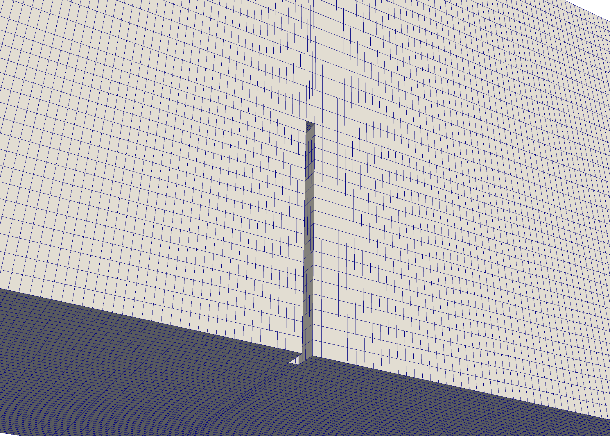
(b)

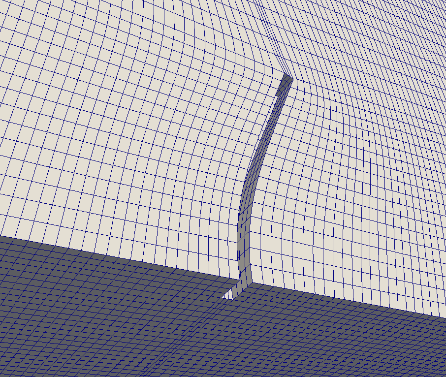
(c)

Figure 1: (a) Sketch of computational domain, (b) part of the undeformend fluid mesh $300k$ and c) one deformed configuration of the same mesh.

Concerning the description of the flow, we consider both the Navier Stokes equations (NSE), i.e. with no LES modeling, and the Leray model implemented through the EFR algorithm. We impose a no slip boundary condition on the channel walls. As for the pressure at the channel walls, we calculate it using a linear extrapolation from the neighboring cell centre. At the inflow, we prescribe a plug flow with horizontal velocity component $U$ at the centerline. At the outflow, we prescribe a null shear stress condition. We start all the simulations from fluid at rest.

We use the following parameters for our simulations: $\rho_{s}=678$ Kg/m³, $\nu_{s}=0.4$, $E=1905.49$ Pa, $U=0.01$ m/s, $\rho_{f}=1000$ Kg/m³, and $\mu_{f}=1e-3$ Pa$\cdot$s to achieve $Re=100$ or $\mu_{f}=2.5e-4$ Pa$\cdot$ s to achieve $Re=400$. These values are taken from [51], where they are stated in dimensionless form though. The quantities of interest for this benchmark are the dimensionless horizontal ($\Delta x/b$) and vertical displacement ($\Delta y/b$) of the midpoint of the structure free edge, and the drag coefficient:

$$c_{d}(t)=\dfrac{2}{\rho_{f}bL{U}^{2}}\int_{S}\left(\boldsymbol{\sigma}_{f}\cdot\boldsymbol{n}\right)\cdot\boldsymbol{t}~{}dS,$$ (38)

where $S$ is the structure surface, and $\boldsymbol{t}$ and $\boldsymbol{n}$ are the tangential and outward normal unit vectors, respectively. Since at $Re=100,400$ the flow evolves towards a steady state, these quantities are computed when the simulation is close enough to steady state [51]. Moreover, for all simulations we evaluate the following errors:

$$E_{c_{d}}=\dfrac{c_{d}-c_{d}^{{true}}}{c_{d}^{{true}}},\quad E_{\Delta x/b}=\dfrac{\Delta x/b-{\Delta x/b}^{{true}}}{{\Delta x/b}^{{true}}},\quad E_{\Delta y/b}=\dfrac{\Delta y/b-{\Delta y/b}^{{true}}}{{\Delta y/b}^{{true}}}.\quad$$ (39)

We consider two different (initially) Cartesian orthogonal meshes for the fluid domain, while we consider only one mesh for the solid domain. The meshes are built by using blockMesh, a mesh generation utility provided in OpenFOAM. Table 1 reports minimum and maximum diameter in the initial configuration, and number of cells for each mesh. Fig. 1 (b) and (c) show part of the fluid mesh $300k$ in the undeformed configuration and one deformed configuration, respectively. We set the time step to 0.01 for all the simulations.

	$h_{min}$	$h_{max}$	No. of cells
Fluid mesh $300k$	6.67e-4	4.4e-3	364008
Fluid mesh $700k$	6.67e-4	3.6e-3	695940
Structure mesh	6.67e-4	2.4e-3	252

Table 1: Minimum diameter $h_{min}$ and maximum diameter $h_{max}$ in the initial configuration, and number of cells for all the meshes under consideration.

A Direct Numerical Simulation (DNS) needs a mesh with spacing close to the Kolmogorov scale $\eta$ [32, 31] that can be expressed as follows:

$$\eta=Re^{-3/4}b.$$ (40)

For our benchmark, we have $\eta=3.16e-4$ at $Re=100$ and $\eta=1.12e-4$ at $Re=400$. The meshes in Table 1 do not feature this level of refinement required by a DNS (especially for $Re=400$), thus the need for LES modeling. We note that the fluid mesh used for the results in [51] has about $6000k$ elements with $h_{min}^{f}=2e-4$ and local refinement such that $h_{min}^{f}\sim\eta$ for all the Reynolds number under consideration. In fact, the results in [51] are obtained with DNS. We choose the under-refined meshes in Table 1 to be able to observe the effect of the filter. As the mesh gets finer and finer (i.e., the mesh size gets closer to the Kolmogorov scale), all the relevant scales become resolved and no filter is needed. The reader interested in learning about the performance of our LES approach for different levels of mesh refinement in fixed domains is referred to [4, 22].

To illustrate the flow field, we show in Figs. 2 and 3 the velocity, pressure, streamlines and vorticity computed by the NSE algorithm close to steady state for $Re=100$ and $Re=400$. The results were obtained with mesh $300k$. As expected, the flow field becomes more complex as the Reynolds number is increased.

\begin{overpic}[width=197.99866pt]{img/u_NSE_100.png} \end{overpic}

\begin{overpic}[width=197.99866pt]{img/p_NSE_100.png} \end{overpic}

\begin{overpic}[width=197.99866pt]{img/streamlines_NSE_100.png} \end{overpic}

\begin{overpic}[width=197.99866pt]{img/vorticity_NSE_100.png} \end{overpic}

Figure 2: Mesh $300k$: Velocity ${\mbox{\boldmath{$u$}}}_{f}$ (top left), pressure $p_{f}$ (top right), streamlines (bottom left) and vorticity (bottom right) fields computed by the NSE algorithm close to steady state for Reynolds number 100.

\begin{overpic}[width=197.99866pt]{img/u_NSE_400.png} \end{overpic}

\begin{overpic}[width=197.99866pt]{img/p_NSE_400.png} \end{overpic}

\begin{overpic}[width=193.60107pt]{img/streamlines_NSE_400.png} \end{overpic}

\begin{overpic}[width=206.80054pt]{img/vorticity_NSE_400.png} \end{overpic}

Figure 3: Mesh $300k$: Velocity ${\mbox{\boldmath{$u$}}}_{f}$ (top left), pressure $p_{f}$ (top right), streamlines (bottom left) and vorticity (bottom right) fields computed by the NSE algorithm close to steady state for Reynolds number 400.

At the numerical level, for all the simulations we fix the number of PISO loops to 3 and non-orthogonal correctors to 1. We use an initial relaxation factor of 0.4 at each time step. For the convective term, we adopt a Central Differencing (CD) scheme [34] in order to avoid introducing stabilization associated with upwind schemes. In this way, we are able to assess the effectiveness of the differential filter. At the end of each FSI iteration, we compute the $L^{2}$-norm of the residual vector on the fluid side of the interface: if this norm falls below 1e-6, then we stop the iterating between fluid and structure solvers for the given time step.

We ran all the simulations in parallel using 20 processor cores. This means about $15k$ cells per CPU for mesh $300k$ and about $35k$ cells per CPU for mesh $700k$, both below the scalability limit for OpenFOAM (i.e., about $50k$ cells per CPU). The simulations are run on SISSA HPC cluster Ulysses, which has recently been upgraded to 200 TFLOPS, 2TB RAM, 7000 cores.

We note that the FSI convergence rate decreases when the Reynolds number increases and during the transition to steady state.

Remark 4.1.

The release of solids4Foam that we used for the results in this paper could not be restarted from a given time step in an efficient way. This issue, that affects both the serial and the parallel versions, is noted also in [38] for an earlier release. The restart introduces a larger error at the FSI interface with respect to the error of an uninterrupted simulation. This generates a localized perturbation in the flow field that spoils the quantities of interest for the benchmark, in particular the drag coefficient. We note that by the time this paper was completed, the developers of solids4foam had uploaded a fix for this problem affecting the restart. However, since such a fix had not been merged with the master branch we chose not to test it.

The restart problem in solids4Foam, together with the maximum wall time of 96 hours allowed for the Ulysses cluster, limited the level of mesh refinement we could afford. An additional difficulty is given by the long time required to reach a quasi steady state condition for the benchmark we consider. For all of these reasons, we consider only the lower Reynolds numbers in [51], and we report only results for the meshes in Table 1. Moreover, for the finer computational mesh we could run only the NSE model.

At $Re=100$, the maximum wall time (96 hours of computations) allows NSE to simulate 85 s of flow with mesh $300k$, while EFR simulates only 61 s. This means that one time step of NSE (resp., EFR) takes in average 40.6 s (resp., 56.6 s). Thus, we estimate that the filter step takes in average 16 s per time step with mesh $300k$ at $Re=100$. This is in line with the times reported in [4]. Recall, that at each time step the fluid and structure problems are solved multiple times. With mesh $700k$, the maximum wall time allows NSE to simulate only 62 s of flow. Considering that the change in the quantities of interest for this benchmark slows down after 55 s of flow for $Re=100$, we did not report the results for EFR with mesh $700k$ as they are not close enough to steady state. We would like to mention that in [44] the authors report over 200 computation hours with solids4Foam to simulate 2.32 seconds of a FSI problem at $Re\sim 2000$ with a Smagorinski-based LES model. They used 20 Intel Xeon CPUs E7- 8870 @ 2.40 GHz processor cores.

Table 2 reports the quantities of interest computed in [51]. In Table 3, the NSE solutions obtained with meshes $300k$ and $700k$ and the EFR solution obtained with mesh $300k$ are compared with the reference values from [51] for $Re=100$ and $Re=400$. For the EFR algorithm, we set $\alpha=h_{min}^{f}$ and the value of $\chi$ has been computed by using the following formula introduced in [22] for flow problems in fixed domain:

$$\chi=\dfrac{h_{min}^{f}-\eta}{\dfrac{\rho_{f}\alpha^{2}}{\mu_{f}\Delta t}\eta-\eta}.$$ (41)

For the current test, we obtain $\chi=0.028$ at $Re=100$ and $\chi=0.0255$ at $Re=400$. From Table 3, we see that the total error $|E_{c_{d}}|+|E_{\Delta x/b}|+|E_{\Delta y/b}|$ for the NSE algorithm decreases as the mesh is refined at a given $Re$ and it increases as $Re$ increases, as one would expect. In addition, we see that the EFR algorithm performs well both for $Re=100$ and $Re=400$: it allows to obtain a smaller total error. Finally, we note that the NSE algorithm with the finer mesh (i.e., $700k$) does not perform as well as the EFR algorithm on the coarser mesh (i.e., $300k$).

$Re$	$c_{d}$	$\Delta x/b$	$\Delta y/b$
100	1.02	2.34	0.67
400	0.94	2.34	0.68

Table 2: Drag coefficient and displacement of the structure free edge reported in [51] for Reynolds numbers 100 and 400.

$Re=100$
Mesh name	Algorithm	$c_{d}$	$\Delta x/b$	$\Delta y/b$	$E_{c_{d}}$	$E_{\Delta x/b}$	$E_{\Delta y/b}$	$\sum_{i}|E_{i}|$
$300k$	NSE	1.24	2.235	0.625	0.216	-0.045	-0.067	0.328
$300k$	EFR	1.236	2.243	0.63	0.212	-0.041	-0.06	0.313
$700k$	NSE	1.239	2.239	0.628	0.215	-0.043	-0.063	0.321
$Re=400$
Mesh name	Algorithm	$c_{d}$	$\Delta x/b$	$\Delta y/b$	$E_{c_{d}}$	$E_{\Delta x/b}$	$E_{\Delta y/b}$	$\sum_{i}|E_{i}|$
$300k$	NSE	0.958	1.809	0.402	0.019	-0.227	-0.409	0.655
$300k$	EFR	0.963	1.842	0.418	0.024	-0.213	-0.385	0.622
$700k$	NSE	1.044	1.903	0.446	0.111	-0.187	-0.344	0.642

Table 3: Quantities of interest and corresponding errors (39) computed with the NSE algorithm (meshes $300k$ and $700k$) and EFR algorithm (mesh $300k$) with $\alpha=h_{min}^{f}$ and $\chi=0.0255$ (Eq. (41)) for $Re=100$ and $Re=400$.

As mentioned above, $\chi$ was set with a formula from [22], where we studied flows at $Re\in[2000,6500]$. This formula might not be optimized for the Reynolds numbers we consider here, as it is likely to introduce more artificial dissipation than needed. This could explain why in Table 3 the error for the drag coefficient is much larger at $Re=100$ than $Re=400$. Once the restart issue mentioned in Remark 4.1 gets fixed, we will work with the higher Reynolds number cases reported in [51], for which we expect our formula to work better.

A key role in the EFR algorithm is played by the indicator function defined in (7). Fig. 4 shows the indicator function computed with the mesh $300k$ close to steady state. We see that the largest values in the region close to and behind the beam, as expected. Additionally, local peaks occur inside the channel boundary layer. Thus, function (7) is a suitable indicator function because it correctly selects the regions of the domain where the velocity does need regularization.

\begin{overpic}[width=197.99866pt]{img/a_EFR_100.png} \put(40.0,50.0){$Re=100$} \end{overpic}

\begin{overpic}[width=197.99866pt]{img/a_EFR_400.png} \put(40.0,50.0){$Re=400$} \end{overpic}

Figure 4: Mesh $300k$: Indicator function computed by the EFR algorithm close to steady state for $Re=100$ (left) and $Re=400$ (right).

5 Conclusions

This paper has two goals: i) to test open source software solids4Foam, which is widely used for FSI simulations; and (ii) assess its flexibility in handling more complex flows. To accomplish such goals, we considered the EFR implementation of a Leray model to study the interaction of an incompressible fluid at moderately large Reynolds numbers with a with a hyperelastic structure modeled as a Saint Venant-Kirchhoff material. We used a strongly coupled, partitioned FSI solver in a finite volume environment, combined with an arbitrary Lagrangian-Eulerian approach to deal with the motion of the fluid domain.

With regard to goal i), we found that solids4Foam is accurate when compared against numerical results in the literature but suffers from a major limitation: the restart function introduces a larger error at the FSI interface, which spoils the restarted simulation. This limits the applicability to problems that can be solved in one run, i.e. simulations over a short period of time. Thus, even simple benchmark tests like the one studied in this article (3D cross flow around an immersed, slender structure [51]) are feasible only at Reynolds numbers of a few hundreds. It appears that a fix to this bug is forthcoming. As for goal ii), we found it relatively easy to replace the standard Navier-Stokes solver with our LES approach within the FSI algorithm. This indicates that solids4Foam is a versatile tool that can easily be extended to more complex fluid (or structure) models.

Disclosure statement

No potential conflict of interest was reported by the author(s).

Funding

This research was funded by the European Research Council Executive Agency by the Consolidator Grant project AROMA-CFD ”Advanced Reduced Order Methods with Applications in Computational Fluid Dynamics” - GA 681447, H2020-ERC CoG 2015 AROMA-CFD, PI G. Rozza, INdAM- GNCS 2019-2020 projects, the US National Science Foundation through grant DMS-1620384 and DMS-195353.

References

- [1] S. Badia, A. Quaini, and A. Quarteroni. Modular vs. non-modular preconditioners for fluid–structure systems with large added-mass effect. Comput. Methods Appl. Mech. Engrg, 197(49):4216 – 4232, 2008.
- [2] K.-J/ Bathe, H. Zhang, and S. Ji. Finite element analysis of fluid flows fully coupled with structural interactions. Computers & Structures, 72(1):1 – 16, 1999.
- [3] Y. Bazilevs, V.M. Calo, J.A. Cottrell, T.J.R. Hughes, A. Reali, and G. Scovazzi. Variational multiscale residual-based turbulence modeling for large eddy simulation of incompressible flows. Computer Methods in Applied Mechanics and Engineering, 197(1):173–201, 2007.
- [4] L. Bertagna, A. Quaini, and A. Veneziani. Deconvolution-based nonlinear filtering for incompressible flows at moderately large Reynolds numbers. International Journal for Numerical Methods in Fluids, 81(8):463–488, 2016.
- [5] J. Borggaard, T. Iliescu, and J.P. Roop. A bounded artificial viscosity large eddy simulation model. SIAM Journal on Numerical Analysis, 47:622–645, 2009.
- [6] A. L. Bowers, L. G. Rebholz, A. Takhirov, and C. Trenchea. Improved accuracy in regularization models of incompressible flow via adaptive nonlinear filtering. International Journal for Numerical Methods in Fluids, 70(7):805–828, 2012.
- [7] M. Breuer, G. De Nayer, M. Münsch, T. Gallinger, and R. Wüchner. Fluid-structure interaction using a partitioned semi-implicit predictor-corrector coupling scheme for the application of large-eddy simulation. Journal of Fluids and Structures, 29:107–130, 02 2012.
- [8] M. Bukac, S. Canic, R. Glowinski, J. Tambaca, and A. Quaini. Fluid–structure interaction in blood flow capturing non-zero longitudinal structure displacement. J. Comp. Phys, 235:515 – 541, 2013.
- [9] H.-J. Bungartz, M. Mehl, and M. Schäfer. Fluid-structure interaction II. Modelling, simulation, optimization. Selected papers based on the presentations at the first international workshop on computational engineering – special topic fluid-structure interactions, Herrsching, Germany, October 2009, volume 73. 01 2010.
- [10] H.-J. Bungartz and M. Schäfer. Fluid-Structure Interaction: Modelling, Simulation, Optimisation. 01 2006.
- [11] E. Burman and M.A. Fernández. Stabilized explicit coupling for fluid-structure interaction using Nitsche’s method. C. R. Acad. Sci. Paris Sér. I Math., 345:467–472, 2007.
- [12] P. Cardiff, A. Karac, P. De Jaeger, H. Jasak, J. Nagy, A. Ivankovic, and Z. Tukovic. An open-source finite volume toolbox for solid mechanics and fluid-solid interaction simulations, 2018.
- [13] P. Causin, J.F. Gerbeau, and F. Nobile. Added-mass effect in the design of partitioned algorithms for fluid-structure problems. Comput. Methods Appl. Mech. Engrg, 194(42-44):4506–4527, 2005.
- [14] J. Degroote and J. Bathe, K.-J.and Vierendeels. Performance of a new partitioned procedure versus a monolithic procedure in fluid–structure interaction. Computers & Structures, 87:793–801, 06 2009.
- [15] J. Degroote, R. Haelterman, S. Annerel, P. Bruggeman, and J. Vierendeels. Performance of partitioned procedures in fluid-structure interaction. Computers & Structures, 88, 04 2010.
- [16] J. Degroote and J. Vierendeels. Multi-solver algorithms for the partitioned simulation of fluid–structure interaction. Computer Methods in Applied Mechanics and Engineering, 200:2195–2210, 06 2011.
- [17] I. Demirdzić and M. Perić. Space conservation law in finite volume calculations of fluid flow. International Journal of Numerical Methods in Fluids, 8:1037–1050, 1988.
- [18] S. Deparis, M. Discacciati, G. Fourestey, and A. Quarteroni. Fluid-structure algorithms based on Steklov-Poincaré operators. Comput. Methods Appl. Mech. Engrg, 195(41-43):5797–5812, 2006.
- [19] M.A. Fernández, J.F. Gerbeau, and C. Grandmont. A projection semi-implicit scheme for the coupling of an elastic structure with an incompressible fluid. C. R. Math. Acad. Sci. Paris, 342:279–284, 2006.
- [20] M.A. Fernández and M. Moubachir. A Newton method using exact Jacobians for solving fluid-structure coupling. Comput. & Structures, 83(2-3):127–142, 2005.
- [21] J.F. Gerbeau and M. Vidrascu. A quasi-Newton algorithm based on a reduced model for fluid-structure interaction problems in blood flows. M2AN Math. Model. Numer. Anal., 37(4):631–648, 2003.
- [22] M. Girfoglio, A. Quaini, and G. Rozza. A finite volume approximation of the navier-stokes equations with nonlinear filtering stabilization. Computers & Fluids, 187:27–45, 2019.
- [23] M. Girfoglio, A. Quaini, and G. Rozza. A POD-Galerkin reduced order model for a LES filtering approach. Journal of Computational Physics, 436:110260, 2021.
- [24] Ma. Heil. An efficient solver for the fully coupled solution of large-displacement fluid–structure interaction problems. Comput. Methods Appl. Mech. Engrg, 193(1):1 – 23, 2004.
- [25] G. Hou, J. Wang, and A. Layton. Numerical methods for fluid-structure interaction — a review. Communications in Computational Physics, 12, 08 2012.
- [26] K. Hughes, R. Vignjevic, J. Campbell, T. Vuyst, N. Djordjevic, and L. Papagiannis. From aerospace to offshore: Bridging the numerical simulation gaps–simulation advancements for fluid structure interaction problems. International Journal of Impact Engineering, 61:48–63, 11 2013.
- [27] T. J. R. Hughes, W. K. Liu, and T. K. Zimmermann. Lagrangian-Eulerian finite element formulation for incompressible viscous flows. Computer Methods in Applied Mechanics and Engineering, 29(3):329–349, 1981.
- [28] J.C. Hunt, A.A. Wray, and P. Moin. Eddies stream and convergence zones in turbulent flows. Technical Report CTR-S88, CTR report, 1988.
- [29] R. I. Issa. Solution of the implicitly discretised fluid flow equations by operator-splitting. Journal of Computational Physics, 62(1):40–65, 1986.
- [30] H. Jasak and Z. Tukovic. Automatic mesh motion for the unstructured finite volume method. Transactions of FAMENA, 30:1–20, 11 2006.
- [31] A. N. Kolmogorov. Dissipation of energy in isotropic turbulence. Doklady Akademii Nauk SSSR, 32:19–21, 1941.
- [32] A. N. Kolmogorov. The local structure of turbulence in incompressible viscous fluids at very large Reynolds numbers. Doklady Akademii Nauk SSSR, 30:301–305, 1941.
- [33] U. Küttler and W. Wall. Fixed-point fluid-structure interaction solvers with dynamic relaxation. Computational Mechanics, 43:61–72, 01 2008.
- [34] P.D. Lax and B. Wendroff. System of conservation laws. Communications on Pure and Applied Mathematics, 13:217–237, 1960.
- [35] W. Layton, L.G. Rebholz, and C. Trenchea. Modular nonlinear filter stabilization of methods for higher Reynolds numbers flow. Journal of Mathematical Fluid Mechanics, 14:325–354, 2012.
- [36] J. Lorentzon and J. Revstedt. A numerical study of partitioned fsi applied to a cantilever in incompressible turbulent flow. International Journal for Numerical Methods in Engineering, 121, 10 2019.
- [37] M. Luhar and H. Nepf. Flow-induced reconfiguration of buoyant and flexible aquatic vegetation. Limnology and Oceanography, 56:2003–2017, 11 2011.
- [38] W. Meng. Analysis on dynamic response of a tension-leg platform riser system. Master’s thesis, Rice University, 2018.
- [39] S. V. Patankar and D. B. Spalding. A calculation procedure for heat, mass and momentum transfer in three-dimensional parabolic flows. International Journal of Heat and Mass Transfer, 15(10):1787–1806, 1972.
- [40] S. Piperno. Explicit/Implicit fluid/structure staggered procedures with a structural predictor and fluid subcycling for 2D inviscid aeroelastic simulations. Int. J. Num. Methods Fluids, 25:1207–1226, 1997.
- [41] S. Piperno, C. Farhat, and B. Larrouturou. Partitioned procedures for the transient solution of coupled aeroelastic problems - Part I: Model problem, theory and two-dimensional application. Comput. Methods Appl. Mech. Engrg, 124:79–112, 1995.
- [42] A. Quaini and A. Quarteroni. A semi-implicit approach for fluid-structure interaction based on an algebraic fractional step method. Math. Models Methods Appl. Sci, 17(06):957–983, 2007.
- [43] A. Quarteroni, R. Sacco, and F. Saleri. Numerical Mathematics. Springer Verlag, 2007.
- [44] K. Rege and B. Hjertager. Application of foam-extend on turbulent fluid-structure interaction. IOP Conference Series Materials Science and Engineering, 276:012031, 12 2017.
- [45] J. Revstedt. Interaction between an incompressible flow and elastic cantilevers of circular cross-section. International Journal of Heat and Fluid Flow, 43:244–250, 10 2013.
- [46] T. Richter. Goal-oriented error estimation for fluid-structure interaction problems. Computer Methods in Applied Mechanics and Engineering, s 223–224, 08 2011.
- [47] T. Richter. A monolithic geometric multigrid solver for fluid-structure interactions in ale formulation. International Journal for Numerical Methods in Engineering, 104, 05 2015.
- [48] I. Sekutkovski, B.and Kostić, A. Simonovic, and V. Cardiff, P.and Jazarević. Three-dimensional fluid–structure interaction simulation with a hybrid rans-les turbulence model for applications in transonic flow domain. Aerospace Science and Technology, 49, 11 2015.
- [49] A.K Slone, K. Pericleous, C. Bailey, M. Cross, and C. Bennett. A finite volume unstructured mesh approach to dynamic fluid-structure interaction: An assessment of the challenge of predicting the onset of flutter. Applied Mathematical Modelling, 28:211–239, 02 2004.
- [50] P. D. Thomas and C. K. Lombard. Geometric conservation law and its application to flow computations on moving grids. AIAA Journal, 17:1030–1037, 1997.
- [51] F.-B. Tian, H. Dai, H. Luo, J. Doyle, and B. Rousseau. Fluid–structure interaction involving large deformations: 3d simulations and applications to biological systems. Journal of Computational Physics, 258:451–469, 02 2014.
- [52] Z. Tukovic and H. Jasak. A moving mesh finite volume interface tracking method for surface tension dominated interfacial fluid flow. Computers & Fluids, 55:70–84, 02 2012.
- [53] Z. Tukovic, A. Karac, P. Cardiff, H. Jasak, and A. Ivankovic. Openfoam finite volume solver for fluid-solid interaction. Transactions of FAMENA, 42:1–31, 10 2018.
- [54] J. P. Van Doormaal and G. D. Raithby. Enhancements of the simple method for predicting incompressible fluid flows. Numerical Heat Transfer, 7(2):147–163, 1984.
- [55] A.W. Vreman. An eddy-viscosity subgrid-scale model for turbulent shear flow: Algebraic theory and applications. Physics of Fluids, 16(10):3670–3681, 2004.
- [56] H. G. Weller, G. Tabor, H. Jasak, and C. Fureby. A tensorial approach to computational continuum mechanics using object-oriented techniques. Computers in physics, 12(6):620–631, 1998.
- [57] L. Zhu, G.-W. He, S. Wang, L. Miller, X. Zhang, Q. You, and S. Fang. An immersed boundary method based on the lattice boltzmann approach in three dimensions, with application. Computers & Mathematics with Applications, 61:3506–3518, 06 2011.