Reversible Random Walks on Dynamic Graphs

Abstract

Recently, random walks on dynamic graphs have been studied because of their adaptivity to the time-varying structure of real-world networks. In general, there is a tremendous gap between static and dynamic graph settings for the lazy simple random walk: Although $O(n^{3})$ cover time was shown for any static graphs of $n$ vertices, there is an edge-changing dynamic graph with an exponential hitting time. On the other hand, previous works indicate that the random walk on a dynamic graph with a time-homogeneous stationary distribution behaves almost identically to that on a static graph. For example, the lazy simple random walk on a dynamic regular graph has an $O(n^{2})$ hitting time, which is the same order as that on a static regular graph.

In this paper, we strengthen this insight by obtaining general and improved bounds. Specifically, we consider a random walk according to a sequence $(P_{t})_{t\geq 1}$ of irreducible and reversible transition matrices such that all $P_{t}$ have the same stationary distribution. We bound the mixing, hitting, and cover times in terms of the hitting and relaxation times of the random walk according to the worst fixed $P_{t}$. Moreover, we obtain the first bounds of the hitting and cover times of multiple random walks and the coalescing time on dynamic graphs. These bounds can be seen as an extension of the well-known bounds of random walks on static graphs. Our results generalize the previous upper bounds for specific random walks on dynamic graphs, e.g., lazy simple random walks and $d_{\max}$-lazy walks, and give improved and tight upper bounds in various cases. As an interesting consequence of our generalization, we obtain tight bounds for the lazy Metropolis walk [Nonaka, Ono, Sadakane, and Yamashita, TCS10] on any dynamic graph: $O(n^{2})$ mixing time, $O(n^{2})$ hitting time, and $O(n^{2}\log n)$ cover time. Additionally, our coalescing time bound implies the consensus time bound of the pull voting on a dynamic graph. To obtain this bound, we establish a duality-like relation of the pull voting process and coalescing random walk on dynamic graphs, which is of independent interest.

Keywords: Random walk, Markov chain, dynamic graph

1 Introduction

A random walk is a fundamental stochastic process on an undirected graph. A walker starts from a specific vertex of a graph. At each discrete time step, a walker moves to a random neighbor. The probability that the walker moves from $u$ to $v$ is given by $P(u,v)$, where the matrix $P\in[0,1]^{V\times V}$ is called transition matrix. Because of their locality, simplicity, and low memory overhead, random walks have a wide range of applications including network analysis, computational complexity, and distributed algorithms [14, 26]. The efficiency of a random walk can be measured by the rate of diffusion, which has been formalized by several notions including mixing time, hitting time and cover time. The mixing time is the time for the distribution of the walker to converge to some limit distribution (called stationary distribution). The hitting time is the maximum expected time of the walker to visit a target vertex where the maximum is taken over the starting and target vertex. The cover time is the expected time of the walker to visit all vertices starting from the worst vertex. The mixing, hitting, and cover times on static graphs have been extensively studied for several decades [3, 30, 35, 9, 23, 36]. For example, Aleliunas, Karp, Lipton, Lovász, and Rackoff [3] proved that the cover time of the simple random walk on any $n$-vertex connected graph is $O(n^{3})$.

Recently, there is a growing interest in a random walk on a dynamic graph since real-world networks change their structure over time [6, 46, 33, 11, 16, 32, 41]. In this setting, at the beginning of the $t$-th round, the walker moves to a random neighbor on the current graph and then the edge set of the graph changes (we assume that the vertex set is static). A central interest is the gap between random walks on a dynamic graph and a static one. Indeed, while the (lazy) simple random walk has an $O(n^{3})$ hitting time for any $n$-vertex static graphs, there is a sequence $(G_{t})_{t\geq 1}$ of connected graphs called the Sisyphus wheel (Figure 1) on which the hitting time is exponential [6].

On the other hand, several researchers observed that random walks on dynamic graphs behave almost identically to that on static graphs if the stationary distribution of a random walk does not change over time [6, 46, 19, 43]. Avin, Koucký, and Lotker [6] considered a random walk called $d_{\max}$-lazy walk which has the uniform stationary distribution on any graph. They proved that the cover time of this walk on any dynamic connected graph is $O(n^{5}\log^{2}n)$, which was later improved by Denysyuk and Rodrigues [19]. Sauerwald and Zanetti [46] considered the lazy simple random walk on a dynamic connected graph with the same time-invariant degree distribution. They obtained tight or nearly-tight bounds for the mixing and hitting times. For example, they showed that both the mixing and hitting times are $O(n^{2})$ on any dynamic regular graph. These bounds are tight up to a constant factor even on static regular graphs. See Section 1.5 for more details about previous works.

Figure 1: The Sisyphus wheel of five vertices. The Sisyphus wheel $\mathcal{G}=(G_{t})_{t\geq 1}$ is defined as follows: For each $t\geq 1$, let $V=V(G_{t})=\{0,\ldots,n-1\}$, $v(t)=t\bmod(n-1)$, and $E(G_{t})=\{\{v(t),i\}:i\in V\setminus\{v(t)\}$. The lazy simple random walk starting from the vertex $0$ of $G_{1}$ has to choose the self-loop for $\Omega(n)$ consecutive times in order to reach the vertex $n-1$. Note that the hitting time of the simple random walk on the Sisyphus wheel is unbounded.

1.1 Our results

In this paper, we support the insight that a random walk on a dynamic graph with the same stationary distribution behaves almost identically to that on a static graph by studying a random walk according to time inhomogeneous transition matrices: Given a sequence of transition matrices $\mathcal{P}=(P_{t})_{t\geq 1}$ where $P_{t}\in[0,1]^{V\times V}$ for all $t$, we consider a random walk according to $\mathcal{P}=(P_{t})_{t\geq 1}$ that is a sequence of random variables $(X_{t})_{t\geq 0}$ satisfying $\mathop{\mathbf{Pr}}[X_{t}=v_{t}|X_{0}=v_{0},\ldots,X_{t-1}=v_{t-1}]=\mathop{\mathbf{Pr}}[X_{t}=v_{t}|X_{t-1}=v_{t-1}]=P_{t}(v_{t-1},v_{t})$ for any $t\geq 1$ and $(v_{0},\ldots,v_{t})\in V^{t+1}$. In other words, at the $t$-th time step ($t\geq 1$), the walker at vertex $u$ randomly selects a vertex according to the distribution $P_{t}(u,\cdot)$. Our interest is to bound the mixing, hitting, cover, and coalescing times under the assumption that all $P_{t}$ has the same stationary distribution.

We briefly introduce essential terminologies to state our results. Let $P\in[0,1]^{V\times V}$ be an irreducible and reversible transition matrix and $\pi\in(0,1]^{V}$ be its stationary distribution. Let $\lambda_{\star}(P)$ denote the second largest eigenvalue in absolute value. Note that $\lambda_{\star}(P)<1$ if $P$ is aperiodic or lazy. Let $t_{\mathrm{rel}}(P)\mathrel{\mathop{:}}=(1-\lambda_{\star}(P))^{-1}$ be the relaxation time of $P$. Let $\mathcal{P}=(P_{t})_{t\geq 1}$ be a sequence of transition matrices. For the random walk $(X_{t})_{t\geq 0}$ according to $\mathcal{P}$, let $t_{\mathrm{hit}}(\mathcal{P})\mathrel{\mathop{:}}=\max_{u,w\in V}\mathop{\mathbf{E}}\left[\min\{t\geq 0:X_{t}=w\}\middle|X_{0}=u\right]$ be the worst-case expected hitting time of $\mathcal{P}$. We sometimes identify $P$ with the sequence $(P_{t})_{t\geq 1}$ of transition matrices with $P_{t}=P$ for all $t\geq 1$. For example, $t_{\mathrm{hit}}(P)$ denotes the hitting time of $\mathcal{P}=(P_{t})_{t\geq 1}$ with all $P_{t}=P$. Let

$$t_{\mathrm{REL}}(\mathcal{P})\mathrel{\mathop{:}}=\max_{t\geq 1}t_{\mathrm{rel}}(P_{t})\hskip 10.00002pt\text{and}\hskip 10.00002ptt_{\mathrm{HIT}}(\mathcal{P})\mathrel{\mathop{:}}=\max_{t\geq 1}t_{\mathrm{hit}}(P_{t}).$$

Mixing time.

Our first result concerns the mixing time. Specifically, for a sequence $\mathcal{P}=(P_{t})_{t\geq 1}$ of transition matrices, a positive probability vector $\pi\in(0,1]^{V}$, and a parameter $\epsilon>0$, we define the uniform mixing time $t_{\mathrm{mix}}^{(\infty,\pi)}(\mathcal{P},\epsilon)$ by

$$t_{\mathrm{mix}}^{(\infty,\pi)}(\mathcal{P},\epsilon)=\min\left\{t\geq 0:\max_{s\geq 0,u,v\in V}\left|\frac{(P_{s+1}P_{s+2}\cdots P_{s+t})(u,v)}{\pi(v)}-1\right|\leq\epsilon\right\}$$ (1)

and let $t_{\mathrm{mix}}^{(\infty,\pi)}(\mathcal{P})\mathrel{\mathop{:}}=t_{\mathrm{mix}}^{(\infty,\pi)}(\mathcal{P},1/2)$. The uniform mixing time $t_{\mathrm{mix}}^{(\infty)}(P,\epsilon)$ for a static Markov chain $P$ can be seen as the mixing time using the $\ell^{\infty}$-norm metric and has been well studied (see, e.g., Section 4.7 in [34]). The intuition behind our definition of $t_{\mathrm{mix}}^{(\infty,\pi)}(\mathcal{P},\epsilon)$ is that the walk mixes well after $t_{\mathrm{mix}}^{(\infty,\pi)}(\mathcal{P},\epsilon)$ steps even if the walker starts at any moment.

As a consequence of the previous work ((3.13) in [43]), we can easily obtain the following uniform mixing time bound.

Proposition 1.1.

Let $\mathcal{P}=(P_{t})_{t\geq 1}$ be a sequence of irreducible, aperiodic, and reversible transition matrices. Suppose that all $P_{t}$ have the same stationary distribution $\pi$. Then, for any $\epsilon>0$, $t_{\mathrm{mix}}^{(\infty,\pi)}(\mathcal{P},\epsilon)=O\left(t_{\mathrm{REL}}(\mathcal{P})\log(\pi_{\min}^{-1}\epsilon^{-1})\right)$, where $\pi_{\min}\mathrel{\mathop{:}}=\min_{v\in V}\pi(v)$.

Proposition 1.1 can be seen as an extension of the well-known mixing time bound $t_{\mathrm{mix}}^{(\infty)}(P,\epsilon)\leq\lceil t_{\mathrm{rel}}(P)\log(\pi_{\min}^{-1}\epsilon^{-1})\rceil$ for static $P$ (Theorem 12.4 in [34]) to the dynamic $\mathcal{P}$.

Our first result is the extension of the following well-known mixing time bound for static $P$ (Theorem 10.22 in [34]): $t_{\mathrm{mix}}^{(\infty)}(P,1/4)\leq 4t_{\mathrm{hit}}(P)+1$.

Theorem 1.2 (Main result 1).

Let $\mathcal{P}=(P_{t})_{t\geq 1}$ be a sequence of irreducible, reversible, and lazy transition matrices. Suppose that all $P_{t}$ have the same stationary distribution $\pi$. Then, for any $0<\epsilon<1$, $t_{\mathrm{mix}}^{(\infty,\pi)}(\mathcal{P},\epsilon)=O\left(t_{\mathrm{HIT}}(\mathcal{P})+t_{\mathrm{REL}}(\mathcal{P})\log\epsilon^{-1}\right)$.

Note that $t_{\mathrm{rel}}(P)\leq t_{\mathrm{hit}}(P)$ holds for any irreducible, reversible and lazy $P$ (Lemma 4.24 in [2]) and thus Theorem 1.2 implies $t_{\mathrm{mix}}^{(\infty,\pi)}(\mathcal{P},1/4)=O\left(t_{\mathrm{HIT}}(\mathcal{P})\right)$. Compared to Proposition 1.1, Theorem 1.2 eliminates the dependency of $\pi_{\min}^{-1}$ in the mixing time bound at the cost of additional $t_{\mathrm{HIT}}$ term and the laziness assumption. Proposition 1.1 gives a better bound if all $P_{t}$ has a small relaxation time (e.g., random walks on expanders). On the other hand, for $\mathcal{P}$ with $t_{\mathrm{REL}}\approx t_{\mathrm{HIT}}$ (e.g., lazy simple random wallk on dynamic cycles, on which both $t_{\mathrm{HIT}}$ and $t_{\mathrm{REL}}$ are $\Theta(n^{2})$), Theorem 1.2 provides a better bound.

Hitting time and cover time.

For the hitting and cover times, we recall an exponential lower bound on the Sisyphus wheel (Figure 1), which implies the following.

Proposition 1.3 ([6]).

There is a sequence of irreducible, reversible, and lazy transition matrices $\mathcal{P}=(P_{t})_{t\geq 1}$ of $t_{\mathrm{hit}}(\mathcal{P})=2^{\Omega(n)}$.

Note that, the sequence $\mathcal{P}$ in Proposition 1.3 has a time-varying stationary distribution. Our second result concerns the hitting and cover times of multiple random walks according to $\mathcal{P}=(P_{t})_{t\geq 1}$, where all $P_{t}$ have the same stationary distribution. For $k\in\mathbb{N}$, let $t_{\mathrm{hit}}^{(k)}(\mathcal{P})$, $t_{\mathrm{cov}}^{(k)}(\mathcal{P})$ denote the worst-case expected hitting and cover times of $k$ independent random walks each is according to $\mathcal{P}$ (see Section 2 for detail). For $\mathcal{P}=(P_{t})_{t\geq 1}$, $\pi\in(0,1]^{V}$ and a parameter $\epsilon>0$, we define the separation time $t_{\mathrm{sep}}^{(\pi)}(\mathcal{P},\epsilon)$ by

$$t_{\mathrm{sep}}^{(\pi)}(\mathcal{P},\epsilon)\mathrel{\mathop{:}}=\min\left\{t\geq 0:\max_{s\geq 0,u,v\in V}\left(1-\frac{(P_{s+1}P_{s+2}\cdots P_{s+t})(u,v)}{\pi(v)}\right)\leq\epsilon\right\}$$ (2)

and let $t_{\mathrm{sep}}^{(\pi)}(\mathcal{P})=t_{\mathrm{sep}}^{(\pi)}(\mathcal{P},1/2)$. If $P_{t}=P$ for all $t\geq 1$, the definition 2 coincides with well-known definition of the separation time for static $P$ in the literature (see, e.g., Section 4.3 in [2]). Note that $t_{\mathrm{sep}}^{(\pi)}(\mathcal{P})\leq t_{\mathrm{mix}}^{(\infty,\pi)}(\mathcal{P})$ by definition.

Theorem 1.4 (Main result 2).

Let $\mathcal{P}=(P_{t})_{t\geq 1}$ be a sequence of irreducible and reversible transition matrices. Suppose that all $P_{t}$ have the same stationary distribution $\pi$. Then, the following holds.

1. $t_{\mathrm{hit}}^{(k)}(\mathcal{P})=O\left(t_{\mathrm{sep}}^{(\pi)}(\mathcal{P})+\frac{t_{\mathrm{HIT}}(\mathcal{P})}{k}\right)$ for any $k\geq 1$. In particular, $t_{\mathrm{hit}}(\mathcal{P})=O\left(t_{\mathrm{HIT}}(\mathcal{P})\right)$ if $P_{t}$ is lazy for all $t\geq 1$.

2. $t_{\mathrm{cov}}^{(k)}(\mathcal{P})=O\left(t_{\mathrm{sep}}^{(\pi)}(\mathcal{P})+\frac{t_{\mathrm{HIT}}(\mathcal{P})\log n}{k}\right)$ for any $k\geq 1$. In particular, $t_{\mathrm{cov}}(\mathcal{P})=O\left(t_{\mathrm{HIT}}(\mathcal{P})\log n\right)$ if $P_{t}$ is lazy for all $t\geq 1$.

Theorem 1.4 is the first result concerning multiple random walks on dynamic graphs. For $k$-independent random walks according to a static $P$, the following bounds are known: $t_{\mathrm{hit}}^{(k)}(P)=O\left(t_{\mathrm{sep}}^{(\pi)}(\mathcal{P})+\frac{t_{\mathrm{hit}}(P)}{k}\right)$ (Theorem 8 in [21]) and $t_{\mathrm{cov}}^{(k)}(P)=O\left(t_{\mathrm{sep}}^{(\pi)}(\mathcal{P})+\frac{t_{\mathrm{hit}}(P)\log n}{k}\right)$ (Theorem 3.2 in [22]). Hence, Theorem 1.4 can be seen as a generalization of these previous bounds. Furthermore, for the case of $k=1$, Theorem 1.4 improves various previous bounds of $t_{\mathrm{hit}}(\mathcal{P})$ and $t_{\mathrm{cov}}(\mathcal{P})$. See Section 1.2 for details.

Meeting time and coalescing time.

Our third result concerns the meeting time $t_{\mathrm{meet}}(\mathcal{P})$ and the coalescing time $t_{\mathrm{coal}}(\mathcal{P})$ of random walks on dynamic graphs. Consider two independent random walks according to the same transition matrix sequence $\mathcal{P}$. The meeting time $t_{\mathrm{meet}}(\mathcal{P})$ is the expected time for the two walkers to meet starting from the worst initial positions. In the coalescing random walk, we consider $|V|$ independent random walks according to $\mathcal{P}$ starting from $|V|$ distinct initial positions. Once two or more walkers gather at the same position, the walkers are merged into one walker. The coalescing time $t_{\mathrm{coal}}(\mathcal{P})$ is the expected time for the $|V|$ walkers to merge into one walker. By definition, we have $t_{\mathrm{meet}}(\mathcal{P})\leq t_{\mathrm{coal}}(\mathcal{P})$ in general.

For any irreducible, reversible, and lazy $P$, it is known that $t_{\mathrm{coal}}(P)=O(t_{\mathrm{hit}}(P))$ (Theorem 1.4 in [40]). Similarly to the hitting time, we observe an exponential gap between static and dynamic settings.

Proposition 1.5.

There is a sequence of irreducible, reversible, and lazy transition matrices $\mathcal{P}=(P_{t})_{t\geq 1}$ satisfying $t_{\mathrm{meet}}(\mathcal{P})=2^{\Omega(n)}$.

Note that Proposition 1.5 also gives an exponential lower bound of the coalescing time since $t_{\mathrm{coal}}(\mathcal{P})\geq t_{\mathrm{meet}}(\mathcal{P})$. The random walk we consider in Proposition 1.5 is the lazy simple random walk on the graph sequence presented by Olshevsky and Tsitsiklis [41], which has an exponential meeting time.

The following main result presents further evidence that that a time-inhomogeneous coalescing walk with a common stationary distribution behaves almost identically to that on a static graph.

Theorem 1.6 (Main result 3).

Let $\mathcal{P}=(P_{t})_{t\geq 1}$ be a sequence of irreducible, reversible, and lazy transition matrices. Suppose that all $P_{t}$ have the same stationary distribution $\pi$. Then, $t_{\mathrm{coal}}(\mathcal{P})=O\left(t_{\mathrm{HIT}}(\mathcal{P})\right)$.

Theorem 1.6 is the first result for the coalescing time on dynamic graphs. Theorem 1.6 generalizes the aforementioned bound of $t_{\mathrm{coal}}(P)=O(t_{\mathrm{hit}}(P))$ for static $P$ (Theorem 1.4 in [40]). Furthermore, Theorem 1.6 plays a key role to bound the consensus time of the pull voting on dynamic graphs (Section 1.3).

1.2 Examples

Our general results Theorems 1.2, 1.4 and 1.6 yield new and improved bounds for mixing, hitting, cover, and coalescing times for various concrete random walks. These consequences are summarized in Table 1. Throughout this section, unless otherwise stated, we assume that a graph $G$ is connected. For a graph $G$ and a vertex $v\in V(G)$, let $N(G,v)$ be the set of neighboring vertices of $v$ (excluding $v$) and $\deg(G,v)=|N(G,v)|$ be the degree of $v$.

		$t_{\mathrm{mix}}^{(\infty,\pi)}$		$t_{\mathrm{hit}}$		$t_{\mathrm{cov}}$
		$O(t_{\mathrm{REL}}\log\pi_{\min}^{-1})$	Pro.1.1
General		$O(t_{\mathrm{HIT}})$	Th.1.2	$O(t_{\mathrm{HIT}})$	Th.1.4	$O(t_{\mathrm{HIT}}\log n)$	Th.1.4
				$O(n^{3}\log n)$	[46]	$O(n^{3}\log^{2}n)$	[46]
	Time hom. deg. dist.	$O(n^{3})$	[46]	$O(n^{3})$	Th.1.4	$O(n^{3}\log n)$	Th.1.4
LS RW	Regular	$O(n^{2})$	[46]	$O(n^{2})$	[46]	$O(n^{2}\log n)$	[46]
		$O(n^{3}\log n)$	[5]	$O(n^{3}\log n)$	[19]
$d_{\max}$ -lazy	Any graph	$O(n^{3})$	Th.1.2	$O(n^{3})$	Th.1.4	$O(n^{3}\log n)$	[19]
LMW	Any graph	$O(n^{2})$	Th.1.2	$O(n^{2})$	Th.1.4	$O(n^{2}\log n)$	Th.1.4

Table 1: Bounds for specific examples that can be obtained from Theorems 1.2 and 1.4. The general results from Propositions 1.1, 1.2 and 1.4 are given in General row. The examples include bounds for a lazy simple random walk (LSRW) on graphs with a time-homogeneous degree distribution, regular graphs, a $d_{\max}$-lazy walk, and a lazy Metropolis walk (LMW). Gray cells mean new or improved bounds.

Lazy simple random walk.

The transition matrix $P_{\mathrm{LS}}(G)$ of the lazy simple random walk on a graph $G$ is defined by $P_{\mathrm{LS}}(G)(u,v)=\frac{1}{2\deg(G,u)}$ if $v\in N(G,u)$, $P_{\mathrm{LS}}(G)(u,u)=1/2$, and $P_{\mathrm{LS}}(G)(u,v)=0$ otherwise. It is well known that $t_{\mathrm{hit}}(P_{\mathrm{LS}}(G))=O(n^{3})$ for any $G$ [3], $t_{\mathrm{hit}}(P_{\mathrm{LS}}(G))=O(n^{2})$ for any regular $G$ [30], and $t_{\mathrm{hit}}(P_{\mathrm{LS}}(G))=O(n)$ for any regular expander $G$ [2].

Let $\mathcal{G}=(G_{t})_{t\geq 1}$ be a sequence of graphs with a time homogeneous degree distribution $(d(v))_{v\in V}$, i.e., $\deg(G_{t},v)=d(v)$ holds for all $t\geq 1$ and $v\in V$. Then, $\mathcal{P}=(P_{\mathrm{LS}}(G_{t}))_{t\geq 1}$ has the common stationary distribution $\pi=\left(\frac{d(v)}{\sum_{u\in V}d(u)}\right)_{v\in V}$. Hence, we can apply Theorems 1.2, 1.4 and 1.6. In particular, Theorem 1.4 implies $t_{\mathrm{hit}}(\mathcal{P})=O(t_{\mathrm{HIT}}(\mathcal{P}))=O(n^{3})$. This improves the $O(n^{3}\log n)$ bound (Main Result 1(3)) of [46]. Another interesting example is the sequence $\mathcal{G}=(G_{t})_{t\geq 1}$ of regular expander graphs. Let $\mathcal{P}=(P_{\mathrm{LS}}(G_{t}))_{t\geq 1}$. For $k=O(n)$, the cover time of $k$ independent lazy simple random walks satisfies $t_{\mathrm{cov}}^{(k)}(\mathcal{P})=O\bigl{(}\frac{n\log n}{k}\bigr{)}$ from Propositions 1.1 and 1.4. This bound is tight since $t_{\mathrm{cov}}^{(k)}(P_{\mathrm{LS}}(G))=\Omega\bigl{(}\frac{n\log n}{k}\bigr{)}$ holds for any (static) $G$ and $k=O(n\log n)$ [42].

$d_{\max}$-lazy walk.

Let $d_{\max}=d_{\max}(G)\mathrel{\mathop{:}}=\max_{v\in V(G)}\deg(v)$ denote the maximum degree of $G$. The transition matrix $P_{\mathrm{DM}}(G)$ of the $d_{\max}$-lazy walk on a graph $G$ is defined by $P_{\mathrm{DM}}(u,v)=\frac{1}{2d_{\max}}$ if $\{u,v\}\in E(G)$, $P_{\mathrm{DM}}(u,u)=1-\frac{\deg(G,u)}{2d_{\max}}$, and $P_{\mathrm{DM}}(G)(u,v)=0$ otherwise. It is known that $t_{\mathrm{hit}}(P_{\mathrm{DM}}(G))=O(n^{3})$ holds for any $G$ ([6, 19]).

Note that $P_{\mathrm{DM}}(G)$ has the uniform stationary distribution for any $G$ since $P_{\mathrm{DM}}(G)$ is symmetric. Hence, for any sequence of graphs $\mathcal{G}=(G_{t})_{t\geq 1}$ and $\mathcal{P}=(P_{\mathrm{DM}}(G_{t}))_{t\geq 1}$, we can apply Theorems 1.2, 1.4 and 1.6. For example, $t_{\mathrm{hit}}(\mathcal{P})=O(t_{\mathrm{HIT}}(\mathcal{P}))=O(n^{3})$ holds from Theorem 1.4. This improves the previous $O(n^{3}\log n)$ bound in [19].

Metropolis walk.

We saw in the previous paragraph that the $d_{\max}$-lazy walk has a polynomial cover time for any dynamic graph. However, as mentioned in [6], the $d_{\max}$-lazy random walk requires knowledge of the maximum degree, which is a global information of $G_{t}$ at each $t\geq 1$. Regarding this issue, we consider the lazy Metropolis walk of Nonaka, Ono, Sadakane, and Yamashita [38]. The transition matrix $P_{\mathrm{LM}}(G)$ of the lazy Metropolis walk on a graph $G$ is defined by

$$P_{\mathrm{LM}}(G)(u,v)=\begin{cases}\frac{1}{2\max\{\deg(G,u),\deg(G,v)\}}&\text{if $\{u,v\}\in E(G)$},\\ 1-\sum_{w\in N(G,u)}\frac{1}{2\max\{\deg(G,u),\deg(G,w)\}}&\text{if $u=v$},\\ 0&\text{otherwise}.\end{cases}$$ (3)

Note that a lazy Metropolis walk uses local degree information around the walker. For any $G$, Nonaka et al. [38] showed $t_{\mathrm{hit}}(P_{\mathrm{LM}}(G))=O(n^{2})$.

Since the transition matrix of the lazy Metropolis walk is symmetric, the stationary distribution is uniform for any underlying graph. Hence, we can apply Theorems 1.2, 1.4 and 1.6. Interestingly, our bounds for Metropolis walks in Table 1 are tight up to a constant factor: On the (static) cycle graph, the lazy Metropolis walk has $\Omega(n^{2})$ mixing time and $\Omega(n^{2})$ hitting time [2]. On the glitter star graph of [38], the lazy Metropolis walk has an $\Omega(n^{2}\log n)$ cover time.

Metropolis walks on edge-Markovian graphs.

Our results concern the sequence of connected graphs. Indeed, it is not difficult to see that Theorems 1.2, 1.4 and 1.6 also hold if $G_{t}$ is connected at least once in every $C$ steps for some positive constant $C$. This setting was already studied in [19]. With some additional arguments, we study random walks on the edge-Markovian graph $(G_{t})_{t\geq 1}$ defined as follows: Let $p,q\in[0,1]$ be parameters and $G_{1}$ be an arbitrary fixed graph. The graph $G_{t+1}$ is obtained by adding each $e\in\binom{V}{2}\setminus E(G_{t})$ independently with probability $p$ and removing each $e\in E(G_{t})$ independently with probability $q$.

The model of edge-Markovian graph was introduced by Clementi, Macci, Monti, Pasquale, and Silvestri [13] as a wide generalization of time-independent dynamic random graphs. Since then, several properties including the flooding [13, 7], rumor spreading [12], and mixing time [11] have been investigated. In this paper, we focus on the Metropolis walk on the edge-Markovian graph $(G_{t})_{t\geq 1}$ and obtain the following result. See Section 7 for the proof.

Theorem 1.7.

Let $c\geq 1$ be arbitrary. Consider $\mathcal{G}(n,p,q)=(G_{t})_{\geq 0}$ the edge-Markovian graph satisfying $\frac{p}{p+q}\geq 32(c+1)\frac{\log n}{n}$ and $0<p+q\leq 1$. Let $\mathcal{P}=(P_{\mathrm{LM}}(G_{t}))_{t\geq 1}$. Then, for any $k\geq 1$, $\mathcal{G}(n,p,q)$ satisfies the following with probability $1-n^{-\Omega(1)}$: $t_{\mathrm{hit}}^{(k)}(\mathcal{P})=O\left(\frac{\max\{1,q/p\}}{p+q}+\log n+\frac{n}{k}\right)$, $t_{\mathrm{cov}}^{(k)}(\mathcal{P})=O\left(\frac{\max\{1,q/p\}}{p+q}+\log n+\frac{n\log n}{k}\right)$ , and $t_{\mathrm{coal}}(\mathcal{P})=O\left(\frac{\max\{1,q/p\}}{p+q}+n\right)$.

1.3 Pull voting on dynamic graphs

In the (weighted) pull voting, we consider an $n$-vertex graph $G=(V,E)$ where each vertex $v\in V$ holds an opinion $\sigma_{v}\in\Sigma$ for a finite set $\Sigma\subseteq\{0,\dots,n-1\}$ of possible opinions. Let $P\in[0,1]^{V\times V}$ be a transition matrix. At every discrete time step, each vertex $u$ chooses a random neighbor according to the distribution $P(u,\cdot)$ and then updates its opinion with the neighbor’s opinion. The aim of the protocol is to reach consensus in which every vertex supports the same opinion. The consensus time $\tau_{\mathrm{cons}}$ is the time of the process to reach consensus.

We consider the pull voting on dynamic graphs. Specifically, let $\mathcal{P}=(P_{t})_{t\geq 1}$ be a transition matrix sequence. In the pull voting according to $\mathcal{P}$, at the $t$-th round, vertices perform the one-round pull voting according to $P_{t}$. We denote by $\tau_{\mathrm{cons}}(\mathcal{P})$ the consensus time of the pull voting according to $\mathcal{P}$ and consider $t_{\mathrm{cons}}(\mathcal{P})\mathrel{\mathop{:}}=\mathop{\mathbf{E}}[\tau_{\mathrm{cons}}(\mathcal{P})]$. Combining Theorem 1.6 and the idea of well-known duality between the coalescing random walk and pull voting [26] with some additional argument, we prove the following.

Theorem 1.8 (Consensus time).

Let $\mathcal{P}=(P_{t})_{t\geq 1}$ be a sequence of irreducible, lazy, and reversible transition matrices. Suppose that all $P_{t}$ have the same stationary distribution $\pi$. Then, $t_{\mathrm{cons}}(\mathcal{P})\leq O(t_{\mathrm{HIT}}(\mathcal{P}))$.

On the other hand, the consensus time can be exponential in general.

Proposition 1.9.

There is a sequence $(G_{t})_{t\geq 1}$ of $n$-vertex connected graphs such that $t_{\mathrm{cons}}(\mathcal{P})=2^{\Omega(n)}$ for $\mathcal{P}=(P_{\mathrm{LS}}(G_{t}))_{t\geq 1}$.

Another important question concerning pull voting is the probability that the process finally agrees with a specific opinion $\sigma\in\Sigma$. Using the voting martingale argument (e.g., [17]), we obtain the following result.

Proposition 1.10 (Winning probability).

Let $\mathcal{P}=(P_{t})_{t\geq 1}$ be a sequence of irreducible, lazy, and reversible transition matrices. Suppose that all $P_{t}$ have the same stationary distribution $\pi$. Consider the pull voting over opinion set $\Sigma$ according to $\mathcal{P}$. Then, the process finally agrees with $\sigma\in\Sigma$ with probability $\sum_{v\in V_{\sigma}}\pi(v)$, where $V_{\sigma}$ is the set of vertices initially holding opinion $\sigma$.

1.4 Proof overview

We overview the proof of the main theorems (Theorems 1.2, 1.4 and 1.6). Throughout this section, we assume that $\mathcal{P}=(P_{t})_{t\geq 1}$ is a sequence of irreducible and reversible transition matrices in which all $P_{t}$ have the same stationary distribution $\pi\in(0,1]^{V}$. For $f,g\in\mathbb{R}^{V}$, define the inner product $\langle\cdot,\cdot\rangle_{\pi}$ as $\langle f,g\rangle_{\pi}=\sum_{v\in V}f(v)g(v)\pi(v)$ and the induced norm $\|f\|_{2,\pi}=\sqrt{\sum_{v\in V}f(v)^{2}\pi(v)}$. Define $\frac{f}{\pi}\in\mathbb{R}^{V}$ by $\left(\frac{f}{\pi}\right)(v)=\frac{f(v)}{\pi(v)}$. Let $\mathbbm{1}$ denote the $|V|$-dimensional all-one vector.

For a vertex $w\in V$, let $D_{w}\in\{0,1\}^{V\times V}$ be the diagonal matrix defined by $D_{w}(v,v)=1$ if $v\neq w$ and $D_{w}(w,w)=0$. We are interested in the substochastic matrix $D_{w}PD_{w}$. Note that $D_{w}PD_{w}$ is the matrix obtained by replacing elements of $P(w,\cdot)$ and $P(\cdot,w)$ with $0$. It is known that $\rho(D_{w}PD_{w})\leq 1-\frac{1}{t_{\mathrm{hit}}(P)}$, where $\rho(M)$ is the spectral radius of $M$ (see Lemma A.1 or Section 3.6.5 in [2]).

Mixing time (Section 3).

Let $\mu_{0}\in[0,1]^{V}$ be an initial distribution and $\mu_{T}=\mu_{0}\prod_{i=1}^{T}P_{i}$ be the distribution of $X_{T}$. Let $d^{(2,\pi)}(\mu_{T})\mathrel{\mathop{:}}=\left\|\frac{\mu_{T}}{\pi}-\mathbbm{1}\right\|_{2,\pi}$, i.e., the $\ell^{2}$-distance between $\mu_{T}/\pi$ and $\mathbbm{1}$. It is known that $\max_{v\in V}\left|\frac{\mu_{T}(v)}{\pi(v)}-1\right|$ can be bounded in terms of $d^{(2,\pi)}(\cdot)$ (see, e.g., [34, 43] or 8). Henceforth, we focus on bounding $d^{(2,\pi)}(\mu_{T})$.

The main part of the proof of Theorem 1.2 is to prove the following inequality: For any $t\geq 0$ and lazy $\mathcal{P}=(P_{t})_{t\geq 1}$, $d^{(2,\pi)}(\mu_{t+1})^{2}\leq d^{(2,\pi)}(\mu_{t})^{2}\left(1-\frac{d^{(2,\pi)}(\mu_{t})^{2}}{t_{\mathrm{HIT}}(\mathcal{P})}\right)$ holds. Applying this inequality repeatedly, we obtain $t_{\mathrm{mix}}^{(\infty,\pi)}(\mathcal{P})=O(t_{\mathrm{HIT}}(\mathcal{P}))$ (see Lemma C.4 or [46] for detail).

The aforementioned inequality comes from a variant of Mihail’s identity (Lemma A.4): For any reversible and lazy $P$ and any probability vector $\mu$, $d^{(2,\pi)}(\mu P)^{2}\leq d^{(2,\pi)}(\mu)^{2}-\mathcal{E}_{P,\pi}(\mu/\pi)$ holds. Here, $\mathcal{E}_{P,\pi}(f)=\frac{1}{2}\sum_{u,v\in V}\pi(u)P(u,v)(f(u)-f(v))^{2}=\langle f,f\rangle_{\pi}-\langle f,Pf\rangle_{\pi}$ is the Dirichlet form of $P$ and $\pi$. In [46], authors consider a lazy simple random walk and give lower bounds of $\mathcal{E}_{P_{\mathrm{LS}},\pi}(\mu/\pi)$ in terms of some graph parameters, e.g., $\mathcal{E}_{P_{\mathrm{LS}},\pi}(\mu/\pi)\geq d^{(2,\pi)}(\mu)^{4}/n^{2}$ for regular graphs. This lower bound means $d^{(2,\pi)}(\mu_{t+1})^{2}\leq d^{(2,\pi)}(\mu_{t})^{2}\left(1-\frac{d^{(2,\pi)}(\mu_{t})^{2}}{n^{2}}\right)$ holds. Our technical contribution is to generalize the previous lower bound of $\mathcal{E}_{P,\pi}(\mu/\pi)$ for any reversible and lazy $P$ in terms of the hitting time (Lemma 3.2): $\mathcal{E}_{P,\pi}(\mu/\pi)\geq d^{(2,\pi)}(\mu)^{4}/t_{\mathrm{hit}}(P)$ holds. This implies the desired inequality, $d^{(2,\pi)}(\mu_{t+1})^{2}\leq d^{(2,\pi)}(\mu_{t})^{2}\left(1-\frac{d^{(2,\pi)}(\mu_{t})^{2}}{t_{\mathrm{HIT}}(\mathcal{P})}\right)$.

The proof of the key lemma (Lemma 3.2) consists of four steps. First, observe that $\mathcal{E}_{P,\pi}(f)=\mathcal{E}_{P,\pi}(-f)$ and $\mathcal{E}_{P,\pi}(f)=\mathcal{E}_{P,\pi}(f+c\mathbbm{1})$ for any $f\in\mathbb{R}^{V}$ and $c\in\mathbb{R}$. Hence, $\mathcal{E}_{P,\pi}(f)=\mathcal{E}_{P,\pi}(f_{\max}\mathbbm{1}-f)$ holds for $f_{\max}\mathrel{\mathop{:}}=\max_{v\in V}f(v)$. Second, let $g\mathrel{\mathop{:}}=f_{\max}\mathbbm{1}-f$. Note that $g(w)=0$ for $w\in V$ satisfying $f(w)=f_{\max}$. Therefore, for any $u,v\in V$, we have $g(v)P(v,u)g(u)=g(v)(D_{w}PD_{w})g(u)$ and thus $\langle g,Pg\rangle_{\pi}=\langle g,D_{w}PD_{w}g\rangle_{\pi}$ holds. Hence, we have $\mathcal{E}_{P,\pi}(g)=\langle g,g\rangle_{\pi}-\langle g,Pg\rangle_{\pi}=\mathcal{E}_{D_{w}PD_{w},\pi}(g)$. Third, from the known inequality $\langle g,D_{w}PD_{w}g\rangle_{\pi}\leq\rho(D_{w}PD_{w})\|g\|_{2,\pi}^{2}$ for the spectral radius (Lemma A.2) and $\rho(D_{w}PD_{w})\leq 1-\frac{1}{t_{\mathrm{hit}}(P)}$ (Lemma A.1), we have $\mathcal{E}_{P,\pi}(g)=\mathcal{E}_{D_{w}PD_{w},\pi}(g)\geq\frac{\|g\|_{2,\pi}^{2}}{t_{\mathrm{hit}}(P)}$. Finally, from a carefully calculation, it is not difficult to see that $\|g\|_{2,\pi}^{2}\geq d^{(2,\pi)}(\mu)^{4}$ for $f=\mu/\pi$.

Hitting and cover times (Section 4).

Let $(X_{t})_{t\geq 0}$ be the random walk according to $\mathcal{P}=(P_{t})_{t\geq 1}$. To obtain an upper bound of the hitting time, it suffices to bound the probability $\mathop{\mathbf{Pr}}\left[\land_{t=0}^{T}\{X_{t}\neq w\}\right]$ for any fixed vertex $w$. Sauerwald and Zanetti [46] used the conditional expectation approach to bound this probability. Instead of this strategy, we use the following key lemma.

Lemma 1.11.

Suppose that $X_{0}$ is sampled from $\pi$. Then, for any vertex $w\in V$ and $T\geq 0$,

$$\mathop{\mathbf{Pr}}\left[\bigwedge_{t=0}^{T}\{X_{t}\neq w\}\right]\leq\prod_{t=1}^{T}\left(1-\frac{1}{t_{\mathrm{hit}}(P_{t})}\right)\leq\exp\left(-\frac{T}{t_{\mathrm{HIT}}(\mathcal{P})}\right).$$

If the walker starts according to the stationary distribution, Lemma 1.11 immediately gives the bounds of the hitting and cover times: Since the event $\land_{t=0}^{T}\{X_{t}\neq w\}$ means that the walk does not hit $w$ until time step $T$, the expected hitting time is upper bounded by $\sum_{T=0}^{\infty}\left(1-\frac{1}{t_{\mathrm{HIT}}(\mathcal{P})}\right)^{T}=t_{\mathrm{HIT}}(\mathcal{P})$. From the union bound, the probability that the cover time is larger than $2t_{\mathrm{HIT}}(\mathcal{P})\log n$ is upper bounded by $n\left(1-\frac{1}{t_{\mathrm{HIT}}(\mathcal{P})}\right)^{2t_{\mathrm{HIT}}(\mathcal{P})\log n}\leq 1/n$. This argument can be easily extended to the case of $k$ independent random walks starting from positions according to the stationary distribution; the expected hitting time is bounded by $\sum_{T=0}^{\infty}\left(1-\frac{1}{t_{\mathrm{HIT}}(\mathcal{P})}\right)^{kT}=O(t_{\mathrm{HIT}}(\mathcal{P})/k)$.

Lemma 1.11 and the bounds of the separation distance (Theorem 1.2) enable us to obtain upper bounds of the hitting and cover times of $k$ walkers from the worst initial positions. Here is the proof sketch. Let $(X_{t}(1),\dots,X_{t}(k))_{t\geq 0}$ be $k$ independent walks starting from the worst initial positions. By definition of the separation distance 2, the probability that the walker $i\in[k]$ is on $u\in V$ at time $t_{\mathrm{sep}}^{(\pi)}(\mathcal{P})$ is $P_{[1,t_{\mathrm{sep}}^{(\pi)}(\mathcal{P})]}(X_{0}(i),u)\geq\frac{1}{2}\pi(u)$. Therefore, in expectation, half of the walkers are distributed according to $\pi$ after $t_{\mathrm{sep}}^{(\pi)}(\mathcal{P})$ steps. From Lemma 1.11, the probability that all of such walkers do not hit a specific vertex $w$ within $T$ steps is at most roughly $(1-1/t_{\mathrm{HIT}}(\mathcal{P}))^{Tk/2}$. Taking $T=O(t_{\mathrm{HIT}}(\mathcal{P})/k)$, this probability can be bounded by some constant probability. This implies $t_{\mathrm{hit}}^{(k)}(\mathcal{P})=O(t_{\mathrm{sep}}^{(\pi)}(\mathcal{P})+t_{\mathrm{HIT}}(\mathcal{P})/k)$ (see Lemma B.1 for detail). The proof for the cover time proceeds in a similar way: From the union bound over $w\in V$, the probability that there is a vertex $w$ such that all the $\pi$-distributed walkers do not hit $w$ within $T$ steps is at most roughly $n(1-1/t_{\mathrm{HIT}}(\mathcal{P}))^{Tk/2}$.

The proof of Lemma 1.11 goes as follows. For a fixed $w\in V$, consider the sequence of substochastic matrices $(D_{w}P_{t}D_{w})_{t\geq 1}$. By definition of $D_{w}$ and the Cauchy–Schwarz inequality, we have $\mathop{\mathbf{Pr}}\left[\bigwedge_{t=0}^{T}\{X_{t}\neq w\}\right]=\sum_{x,y\in V}\pi(x)\left(\prod_{t=1}^{T}(D_{w}P_{t}D_{w})\right)(x,y)\leq\left\|\left(\prod_{t=1}^{T}(D_{w}P_{t}D_{w})\right)\mathbbm{1}\right\|_{2,\pi}$. Furthermore, from the reversibility of $P_{t}$, all $D_{w}P_{t}D_{w}$ are reversible. Thus we can apply a variant of the Courant–Fischer theorem for the $\pi$-inner product (Lemma A.2) repeatedly and obtain $\left\|\left(\prod_{t=1}^{T}(D_{w}P_{t}D_{w})\right)\mathbbm{1}\right\|_{2,\pi}\leq\prod_{t=1}^{T}\rho(D_{w}P_{t}D_{w})$. Since $\rho(D_{w}PD_{w})\leq 1-1/t_{\mathrm{hit}}(P)$ (Lemma A.1), we obtain Lemma 1.11.

Meeting and coalescing times (Section 5).

To give an upper bound of the coalescing time, we recall the powerful Meeting Time Lemma given by Oliveira [39] (for continuous-time walks) and Oliveira and Peres [40] (for discrete-time lazy walks). These are originally results for time-homogeneous random walks. Our key observation is that Meeting Time Lemma indeed holds for time-inhomogeneous random walks with the same stationary distribution. Suppose that $\mathcal{P}$ is lazy (Note that Lemma 1.11 does not need the laziness assumption).

Lemma 1.12.

Suppose that $X_{0}$ is sampled from $\pi$. Then, for any sequence of vertices $(w_{t})_{t\geq 0}$,

$$\mathop{\mathbf{Pr}}\left[\bigwedge_{t=0}^{T}\{X_{t}\neq w_{t}\}\right]\leq\prod_{t=1}^{T}\left(1-\frac{1}{t_{\mathrm{hit}}(P_{t})}\right)\leq\exp\left(-\frac{T}{t_{\mathrm{HIT}}(\mathcal{P})}\right).$$

Suppose that the initial positions of two independent random walks $(X_{t}(1))_{t\geq 0}$ and $(X_{t}(2))_{t\geq 0}$ are according to the stationary distribution. Lemma 1.12 gives an upper bound of the probability that two walkers do not meet in the dynamic setting: $\mathop{\mathbf{Pr}}\left[\land_{t=0}^{T}\{X_{t}(1)\neq X_{t}(2)\}\right]\leq\exp\left(-\frac{T}{t_{\mathrm{HIT}}(\mathcal{P})}\right)$, i.e., the expected meeting time is upper bounded by $t_{\mathrm{HIT}}(\mathcal{P})$. Note that $\mathop{\mathbf{Pr}}\left[\land_{t=0}^{T}\{X_{t}(1)\neq X_{t}(2)\}\right]\leq\mathop{\mathbf{Pr}}\left[\land_{t=0}^{T}\{X_{t}(1)\neq w_{t})\}\right]$ holds for some sequence of vertices $(w_{t})_{t\geq 0}$.

The proof of our $O(t_{\mathrm{HIT}}(\mathcal{P}))$ coalescing time bound essentially consists of three parts. In the first part, we bound the probability that coalescing time is larger than $Ct_{\mathrm{HIT}}(\mathcal{P})$ for a suitable constant $C>0$ in terms of the probability of a suitable event of independent multiple random walks (Lemma 5.3). This part proceeds similarly to the argument of static setting in [40] by coupling arguments. In the second part, similar to the arguments of multiple random walks, we show that the positions of an appropriate group of walkers at $t=t_{\mathrm{sep}}^{(\pi)}(\mathcal{P})$ are according to the stationary distribution with constant probability. In the third part, we apply Lemma 1.12 to such group of walkers (Lemma 5.4). Since Lemma 1.12 works in the dynamic setting, we can complete this part in a similar way to the static setting [40].

In the proof of Lemma 1.12, the laziness assumption of walkers is essential as well as that of [40]. Since $P$ is positive semidefinite by the laziness, we rewrite $D_{x}PD_{y}=D_{x}\sqrt{P}\sqrt{P}D_{y}$, where $\sqrt{P}$ is the square root of $P$. Furthermore, the reversibility of $P$ implies that $D_{x}\sqrt{P}$ is the adjoint of $\sqrt{P}D_{x}$ (that is, $\pi(u)(D_{x}\sqrt{P})(u,v)=\pi(v)(\sqrt{P}D_{x})(v,u)$ for any $u,v\in V$). Hence, we have $\|D_{x}PD_{y}f\|_{2,\pi}\leq\sqrt{\rho(D_{x}PD_{x})\rho(D_{y}PD_{y})}\|f\|_{2,\pi}\leq\left(1-\frac{1}{t_{\mathrm{hit}}(P)}\right)\|f\|_{2,\pi}$ for any vector $f$ (Lemmas A.5 and A.1). Combining this inequality and similar arguments in the proof of Lemma 1.11, we obtain $\mathop{\mathbf{Pr}}\left[\bigwedge_{t=0}^{T}\{X_{t}\neq w_{t}\}\right]\leq\left\|\left(\prod_{t=1}^{T}(D_{w_{t-1}}P_{t}D_{w_{t}})\right)\mathbbm{1}\right\|_{2,\pi}\leq\prod_{t=1}^{T}\left(1-\frac{1}{t_{\mathrm{hit}}(P_{t})}\right)$.

1.5 Related work

Random walk on a static graph.

Consider a simple random walk on a connected graph $G$ of $n$ vertices and $m$ edges. Aleliunas, Karp, Lipton, Lovász, and Rackoff [3] showed that the cover time is at most $2m(n-1)$. Kahn, Linial, Nisan, and Saks [30] showed that the cover time is at most $16mn/d_{\min}$, while the hitting time is at least $(1/2)m/d_{\min}$ (see Corollary 3.3 of Lovász [35]). Brightwell and Winkler [9] presented the lollipop graph on which the hitting time is approximately $(4/27)n^{3}$ as $n$ increases, while Feige [23] gave proved that the cover time is $(4/27)n^{3}+O(n^{5/2})$ for any graph. In addition to the trivial relation of $t_{\mathrm{hit}}\leq t_{\mathrm{cov}}$, it is known that $t_{\mathrm{cov}}\leq t_{\mathrm{hit}}\log n$ holds for any $G$ (see Matthews [36]).

The cover time $t_{\mathrm{cov}}^{(k)}$ of $k$ independent simple random walks has been investigated in [10, 4, 22, 21, 42]. If $k$ walkers start from the stationary distribution, Broder, Karlin, Raghavan, and Upfal [10] showed that the cover time is at most $O\bigl{(}\left(\frac{m}{k}\right)^{2}\log^{3}n\bigr{)}$. Very recently, Rivera, Sauerwald, and Sylvester [42] proved an improved bound of $O\bigl{(}\bigl{(}\frac{m}{kd_{\min}}\bigr{)}^{2}\log^{2}n\bigr{)}$. From the worst initial positions of $k$ walkers, Elsässer and Sauerwald [22] showed that $t_{\mathrm{cov}}^{(k)}=O\left(t_{\mathrm{mix}}+\frac{t_{\mathrm{hit}}\log n}{k}\right)$ for $k\leq n$.

It is known that local degree information provides surprising power with random walks. For example, the $\beta$-random walk proposed by Ikeda, Kubo, Okumoto, and Yamashita [28, 29] and the Metropolis walk proposed by Nonaka, Ono, Sadakane, and Yamashita ([38], the definition is 3) have the $O(n^{2})$ hitting time and $O(n^{2}\log n)$ cover time for any $G$. These bounds improve the worst-case $\Omega(n^{3})$ hitting time of the simple random walk (on the lollipop graph). Recently, David and Feige [18] showed the $O(n^{2})$ cover time for the minimum-degree random walk proposed by Abdullah, Cooper, and Draief [1]. This is best possible since any random walk on the path has $\Omega(n^{2})$ cover time [29]. It is easy to see that the $\beta$-random walk and the minimum-degree random walk have exponential hitting times on the Sisyphus wheel.

The meeting and coalescing times have been well investigated in the context of distributed computation such as leader election and consensus protocols [26]. Consider the simple random walk on a connected and nonbipartite $G$. Tetali and Winkler showed that the meeting time is at most $(16/27+o(1))n^{3}$. Hassin and Peleg [26] showed $t_{\mathrm{coal}}\leq t_{\mathrm{meet}}\log n$, while $t_{\mathrm{meet}}\leq t_{\mathrm{coal}}$ is trivial. Recent works on the meeting and coalescing times consider the lazy simple random walk on a connected graph $G$ [15, 8, 31, 40]. For example, Kanade, Mallmann-Trenn, and Sauerwald [31] showed $t_{\mathrm{coal}}=O\left(t_{\mathrm{meet}}\left(1+\sqrt{\frac{t_{\mathrm{mix}}}{t_{\mathrm{meet}}}}\log n\right)\right)$. Oliveira and Peres [40] proved $t_{\mathrm{coal}}=O(t_{\mathrm{hit}})$.

Random walk on dynamic graphs.

Avin, Koucký and Lotker [6] presented the Sisyphus wheel on which the hitting time is $2^{\Omega(n)}$ for the lazy simple random walk (Figure 1). To avoid the issue of the exponential hitting time, Avin et al. [6] considered the $d_{\max}$-lazy random walk on $G$ and showed that the cover time of this random walk on any sequence of connected graphs is $O(n^{5}\log^{2}n)$. They also showed that the mixing time of the walk is $O(n^{3}\log n)$. Denysyuk and Rodrigues [19] improved the bound of the cover time to $O(n^{3}\log n)$. Sauerwald and Zanetti [46] considered a lazy simple random walk on a sequence $(G_{t})_{t\geq 1}$ of graphs such that all $G_{t}$ have a common degree distribution. They showed that the $O(n/\pi_{\min})$ mixing time and $O((n\log n)/\pi_{\min})$ hitting time. Moreover, if all $G_{t}$ are $d$-regular, then the hitting time is $O(n^{2})$. This bound matches that of static regular graphs [30].

The study of time inhomogeneous Markov chains has applications in a wide range of fields, including consensus algorithm [41] and cryptography [37]. In an early work, Griffeath [25] studied the ergodic theorem of time inhomogeneous Markov chains. Saloff-Conste and Zúñiga [44, 45] considered the merging time for time inhomogeneous Markov chains in terms of the stability of stationary distributions. In another paper [43], they obtained an upper bound of the mixing time for time inhomogeneous Markov chains under the assumption that the chains are irreducible and have a common stationary distribution.

Cai, Sauerwald, and Zaneti [11] considered the lazy simple random walk on a sequence of edge-Markovian random graphs. They introduced the notion of mixing time on this sequence (note that the stationary distribution changes over time) and obtained several mixing time bounds. Lamprou, Martin, and Spirakis [33] studied the cover time of the simple random walk on a variant of edge-Markovian random graphs.

Pull voting.

The pull voting according to $P_{\mathrm{LS}}(G)$ for a static graph $G$ has been intensively studied [26, 15] in the literature of distributed computing and stochastic process. It is widely known that the consensus time and the coalescing time are equal. Therefore, bounds for coalescing time yields bounds for consensus time. In particular, the consensus time on any (static) connected nonbipartite graphs is $O(n^{3}\log n)$ from Hassin and Peleg [26].

Berenbrink, Giakkoupis, Kermarrec, and Mallmann-trenn [8] studied the pull voting according to $(P_{\mathrm{LS}}(G_{t}))_{t\geq 1}$ for a sequence $(G_{t})_{t\geq 1}$ of graphs constructed by an adaptive adversary. That is, for every $t$, the graph $G_{t}$ can depend on the history of opinion configurations. Under the assumption that all $G_{t}$ must have the same degree distribution, they obtained an upper bound of $\tau_{\mathrm{cons}}$ in terms of the conductance of $G_{t}$ for the binary opinion setting (i.e., $|\Sigma|=2$).

2 Notations and definitions

This section defines the mixing, hitting, cover, meeting, and coalescing times formally. For $b\geq a\geq 1$ and a sequence $(P_{t})_{t\geq 1}$ of transition matrices, let $P_{[a,b]}\mathrel{\mathop{:}}=P_{a}P_{a+1}\cdots P_{b}$. For $\pi\in[0,1]^{V}$, let $\pi_{\min}\mathrel{\mathop{:}}=\min_{v\in V}\pi(v)$.

For $p\geq 1$ and probability vectors $\mu\in[0,1]^{V}$ and $\pi\in(0,1]^{V}$, let

$$d^{(p,\pi)}(\mu) \mathrel{\mathop{:}}=\begin{cases}\left\|\frac{\mu}{\pi}-\mathbbm{1}\right\|_{p,\pi}=\left(\sum_{v\in V}\pi(v)\left|\frac{\mu(v)}{\pi(v)}-1\right|^{p}\right)^{1/p}&\text{if }1\leq p<\infty,\\ \max_{v\in V}\left|\frac{\mu(v)}{\pi(v)}-1\right|&\text{if }p=\infty\end{cases}$$

be the $\ell^{p}$-distance between $\mu/\pi$ and $\mathbbm{1}$. It is known that $d^{(p,\pi)}(\mu)\leq d^{(p+1,\pi)}(\mu)$ holds for any $p\geq 1$ (see, e.g., Section 4.7 in [34]). For example, $\sum_{v\in V}|\mu(v)-\pi(v)|=d^{(1,\pi)}(\mu)\leq d^{(2,\pi)}(\mu)\leq d^{(\infty,\pi)}(\mu)$. For $\mathcal{P}=(P_{t})_{t\geq 1}$, a probability vector $\pi\in(0,1]^{V}$, and $\epsilon>0$, we define the $\ell^{p}$-mixing time as

$$t_{\mathrm{mix}}^{(p,\pi)}(\mathcal{P},\epsilon)\mathrel{\mathop{:}}=\min\left\{t\geq 0:\max_{s\geq 1,v\in V}d^{(p,\pi)}\left(P_{[s+1,s+t]}(v,\cdotp)\right)\leq\epsilon\right\}.$$

Write $t_{\mathrm{mix}}^{(p,\pi)}(\mathcal{P})\mathrel{\mathop{:}}=t_{\mathrm{mix}}^{(p,\pi)}(\mathcal{P},1/2)$.

Consider $k$ independent random walks $(X_{t}(1))_{t\geq 0},\ldots,(X_{t}(k))_{t\geq 0}$, where each walk is according to $\mathcal{P}=(P_{t})_{t\geq 1}$. Let $\tau_{\mathrm{hit}}^{(k)}(\mathcal{P},w)$ (for $w\in V$) and $\tau_{\mathrm{cov}}^{(k)}(\mathcal{P})$ be the random variables denoting hitting and cover times of the $k$ random walks, respectively. Formally,

$$\tau_{\mathrm{hit}}^{(k)}(\mathcal{P},w) =\inf\left\{t\geq 0:\bigcup_{i\in[k],0\leq s\leq t}\{X_{s}(i)\}\ni w\right\},$$ (4)

$$\tau_{\mathrm{cov}}^{(k)}(\mathcal{P}) =\inf\left\{t\geq 0:\bigcup_{i\in[k],0\leq s\leq t}\{X_{s}(i)\}=V\right\}.$$ (5)

Let $t_{\mathrm{hit}}^{(k)}(\mathcal{P})\mathrel{\mathop{:}}=\max_{x\in V^{k},w\in V}\mathop{\mathbf{E}}\left[\tau_{\mathrm{hit}}^{(k)}(\mathcal{P},w)\middle|X_{0}=x\right]$ for the expected hitting time of $k$ random walks. Here, $X_{t}=(X_{t}(1),\ldots,X_{t}(k))\in V^{k}$ is a vector-valued random variable. Similarly, the expected cover time of $k$ random walks is defined by $t_{\mathrm{cov}}^{(k)}(\mathcal{P})\mathrel{\mathop{:}}=\max_{x\in V^{k}}\mathop{\mathbf{E}}\left[\tau_{\mathrm{cov}}^{(k)}(\mathcal{P})\middle|X_{0}=x\right]$. In particular, let $t_{\mathrm{hit}}(\mathcal{P})=t_{\mathrm{hit}}^{(1)}(\mathcal{P})$ and $t_{\mathrm{cov}}(\mathcal{P})=t_{\mathrm{cov}}^{(1)}(\mathcal{P})$.

Let $(X_{t}(1))_{t\geq 0}$ and $(X_{t}(2))_{t\geq 0}$ be two independent random walks, where each walker is according to $\mathcal{P}=(P_{t})_{t\geq 1}$. Write $X_{t}=(X_{t}(1),X_{t}(2))\in V^{2}$. Then, let $\tau_{\mathrm{meet}}(\mathcal{P})\mathrel{\mathop{:}}=\min\{t\geq 0:X_{t}(1)=X_{t}(2)\}$ and define the meeting time of $\mathcal{P}$ as $t_{\mathrm{meet}}(\mathcal{P})\mathrel{\mathop{:}}=\max_{x\in V^{2}}\mathop{\mathbf{E}}\left[\tau_{\mathrm{meet}}(\mathcal{P})\middle|X_{0}=x\right]$.

Let $(\mathrm{C}_{t}(1))_{t\geq 0},(\mathrm{C}_{t}(2))_{t\geq 0},\ldots,(\mathrm{C}_{t}(n))_{t\geq 0}$ denote the coalescing random walks according to $\mathcal{P}=(P_{t})_{t\geq 1}$. In the coalescing random walks, once two or more walkers meet at the same vertex, they merge into one walker. Formally, from a given initial state $\mathrm{C}_{0}=(\mathrm{C}_{0}(1),\ldots,\mathrm{C}_{0}(n))\in V^{n}$, we inductively determine $\mathrm{C}_{t}(a)$ for each $t\geq 1$ and $a\in[n]$, as follows. Suppose that $\mathrm{C}_{t-1}=(\mathrm{C}_{t-1}(1),\ldots,\mathrm{C}_{t-1}(n))$ and $\mathrm{C}_{t}(1),\ldots,\mathrm{C}_{t}(a-1)$ are determined. If there is some $b<a$ such that $\mathrm{C}_{t-1}(a)=\mathrm{C}_{t-1}(b)$, let $\mathrm{C}_{t}(a)\mathrel{\mathop{:}}=\mathrm{C}_{t}(b)$. Otherwise, $\mathrm{C}_{t}(a)$ is determined by the random walk according to $P_{t}$, i.e., $\mathop{\mathbf{Pr}}[\mathrm{C}_{t}(a)=v|\mathrm{C}_{t-1}(a)=u]=P_{t}(u,v)$ for $u,v\in V$. For $x=(x_{1},x_{2},\ldots,x_{n})\in V^{n}$, let $S(x)\mathrel{\mathop{:}}=\bigcup_{i=1}^{n}\{x_{i}\}$ (e.g., $S(x)=\{a,b\}$ for $x=(a,a,b)$). Then, let $\tau_{\mathrm{coal}}(\mathcal{P})=\min\{t\geq 0:|S(\mathrm{C}_{t})|=1\}$ and define the coalescing time of $\mathcal{P}$ as $t_{\mathrm{coal}}(\mathcal{P})\mathrel{\mathop{:}}=\max_{x\in V^{n}}\mathop{\mathbf{E}}[\tau_{\mathrm{coal}}(\mathcal{P})|\mathrm{C}_{0}=x]$.

3 Mixing time

In this section, we show the following lemma, which immediately yields Theorem 1.2.

Lemma 3.1.

Let $\mathcal{P}=(P_{t})_{t\geq 1}$ be a sequence of irreducible, reversible, and lazy transition matrices. Suppose that all $P_{t}$ have the same stationary distribution $\pi$. Then, for any $u,v\in V$ and any $0<\epsilon<1$, $\left|\frac{P_{[1,2T]}(u,v)}{\pi(v)}-1\right|\leq\epsilon^{2}$ holds if $T\geq\frac{\mathrm{e}^{2}}{\mathrm{e}-1}t_{\mathrm{HIT}}(\mathcal{P})+2\log(4t_{\mathrm{HIT}}(\mathcal{P}))+1+t_{\mathrm{REL}}(\mathcal{P})\log\epsilon^{-1}$.

To show Lemma 3.1, we introduce some terminology. Let $\pi\in(0,1]^{V}$ be a positive probability distribution and $f\in\mathbbm{R}^{V}$ be a vector. Then, let $\mathop{\mathbf{E}}_{\pi}(f)\mathrel{\mathop{:}}=\sum_{v\in V}\pi(v)f(v)=\langle f,\mathbbm{1}\rangle_{\pi}$ and $\mathop{\mathbf{Var}}_{\pi}(f)\mathrel{\mathop{:}}=\sum_{v\in V}\pi(v)(f(v)-\mathop{\mathbf{E}}_{\pi}(f))^{2}=\langle f,f\rangle_{\pi}-\langle f,\mathbbm{1}\rangle_{\pi}^{2}$. Note that, for any probability vector $\mu\in[0,1]^{V}$, we have

$$d^{(2,\pi)}(\mu)^{2}=\sum_{v\in V}\pi(v)\left(\frac{\mu(v)}{\pi(v)}-1\right)^{2}=\sum_{v\in V}\pi(v)\left(\frac{\mu(v)}{\pi(v)}\right)^{2}-1=\mathop{\mathbf{Var}}_{\pi}\left(\frac{\mu}{\pi}\right).$$

For a transition matrix $P$ such that $\pi(u)P(u,v)=\pi(v)P(v,u)$ holds for all $u,v\in V$, let $\mathcal{E}_{P,\pi}(f)\mathrel{\mathop{:}}=\langle f,f\rangle_{\pi}-\langle f,Pf\rangle_{\pi}=\frac{1}{2}\sum_{u,v\in V}\pi(u)P(u,v)(f(u)-f(v))^{2}$ be the Dirichlet form.

3.1 Key lemma

The following key lemma connects the Dirichlet form, $\ell^{2}$-distance, and hitting time.

Lemma 3.2.

Let $\mathcal{P}=(P_{t})_{t\geq 1}$ be a sequence of irreducible, reversible, and lazy transition matrices. Suppose that all $P_{t}$ have the same stationary distribution $\pi$. Then, for any probability vector $\mu\in[0,1]^{V}$,

$$\mathcal{E}_{P,\pi}\left(\frac{\mu}{\pi}\right)\geq\frac{\mathop{\mathbf{Var}}_{\pi}\left(\frac{\mu}{\pi}\right)^{2}}{t_{\mathrm{hit}}(P)}.$$

Proof.

Write $f=\frac{\mu}{\pi}$ and let $f_{\max}\mathrel{\mathop{:}}=\max_{v\in V}f(v)$ and $g\mathrel{\mathop{:}}=f_{\max}\mathbbm{1}-f$. Since $f(u)-f(v)=g(v)-g(u)$ for any $u,v\in V$, we have

$$\mathcal{E}_{P,\pi}(f)=\frac{1}{2}\sum_{u,v\in V}\pi(u)P(u,v)(f(u)-f(v))^{2}=\mathcal{E}_{P,\pi}(g)=\langle g,g\rangle_{\pi}-\langle Pg,g\rangle_{\pi}.$$

Let $v_{\max}$ denote a vertex satisfying $f(v_{\max})=f_{\max}$. Recall that $D_{w}\in\{0,1\}^{V\times V}$ is a diagonal matrix where $D_{w}(v,v)\mathrel{\mathop{:}}=\mathbbm{1}_{v\neq w}$ for all $v\in V$. From Lemmas A.2 and A.1, we have

$$\langle Pg,g\rangle_{\pi} =\langle D_{v_{\max}}PD_{v_{\max}}g,g\rangle_{\pi}\leq\rho(D_{v_{\max}}PD_{v_{\max}})\langle g,g\rangle_{\pi}\leq\left(1-\frac{1}{t_{\mathrm{hit}}(P)}\right)\langle g,g\rangle_{\pi}.$$

Note that we have $g(u)P(u,v)g(v)=g(u)(D_{v_{\max}}PD_{v_{\max}})(u,v)g(v)$ holds for any $u,v\in V$. Furthermore,

$$\langle g,g\rangle_{\pi} =\sum_{v\in V}\pi(v)(f_{\max}-f(v))^{2}=\sum_{v\in V}\pi(v)(f_{\max}-1+1-f(v))^{2}$$

$$=(f_{\max}-1)^{2}+\sum_{v\in V}\pi(v)(1-f(v))^{2}\geq\mathop{\mathbf{Var}}_{\pi}\left(f\right)^{2}+\mathop{\mathbf{Var}}_{\pi}\left(f\right).$$

The last inequality follows from $0\leq\mathop{\mathbf{Var}}_{\pi}\left(f\right)=\sum_{v\in V}\pi(v)\left(\frac{\mu(v)}{\pi(v)}\right)^{2}-1\leq f_{\max}-1$. Therefore, we obtain

$$\mathcal{E}_{P,\pi}(f) =\langle g,g\rangle_{\pi}-\langle Pg,g\rangle_{\pi}\geq\frac{\langle g,g\rangle_{\pi}}{t_{\mathrm{hit}}(P)}\geq\frac{\mathop{\mathbf{Var}}_{\pi}\left(f\right)^{2}}{t_{\mathrm{hit}}(P)}.$$

∎

3.2 Upper bound of mixing time

To show Lemma 3.1, we introduce the following bound shown in [43].

Lemma 3.3 ([43]).

Let $\mathcal{P}=(P_{t})_{t\geq 1}$ be a sequence of irreducible, aperiodic, and reversible transition matrices. Suppose that all $P_{t}$ have the same stationary distribution $\pi$. Then, for any probability vector $\mu\in[0,1]^{V}$,

$$d^{(2,\pi)}\left(\mu P_{[1,T]}\right) \leq d^{(2,\pi)}(\mu)\prod_{t=1}^{T}\lambda_{\star}(P_{t})\leq d^{(2,\pi)}(\mu)\exp\left(-\frac{T}{t_{\mathrm{REL}}(\mathcal{P})}\right).$$

Proof.

Applying Lemma A.3 repeatedly to $d^{(2,\pi)}\left(\mu P_{[1,T]}\right)=\left\|\frac{\mu P_{[1,T]}}{\pi}-\mathbbm{1}\right\|_{2,\pi}$, we have

$$\left\|\frac{\mu P_{[1,T]}}{\pi}-\mathbbm{1}\right\|_{2,\pi}\leq\left\|\frac{\mu P_{[1,T-1]}}{\pi}-\mathbbm{1}\right\|_{2,\pi}\lambda_{\star}(P_{T})\leq\cdots\leq\left\|\frac{\mu}{\pi}-\mathbbm{1}\right\|_{2,\pi}\prod_{t=1}^{T}\lambda_{\star}(P_{t}).$$

Then, since

$$\prod_{t=1}^{T}\lambda_{\star}(P_{t})=\prod_{i=1}^{T}\left(1-\frac{1}{t_{\mathrm{rel}}(P_{t})}\right)\leq\exp\left(-\sum_{t=1}^{T}\frac{1}{t_{\mathrm{rel}}(P_{t})}\right)\leq\exp\left(-\frac{T}{t_{\mathrm{REL}}(\mathcal{P})}\right)$$

holds, we obtain the claim. ∎

Combining Lemmas 3.3 and 3.2, we obtain the following bounds of $\ell^{2}$-distance.

Lemma 3.4.

Let $\mathcal{P}=(P_{t})_{t\geq 1}$ be a sequence of irreducible, reversible, and lazy transition matrices. Suppose that all $P_{t}$ have the same stationary distribution $\pi$. Then, for any probability distribution $\mu\in[0,1]^{V}$ and any $0<\epsilon<1$, $d^{(2,\pi)}(\mu P_{[1,T]})\leq\epsilon$ holds if $T\geq\frac{\mathrm{e}^{2}}{\mathrm{e}-1}t_{\mathrm{HIT}}(\mathcal{P})+2\log(4t_{\mathrm{HIT}}(\mathcal{P}))+1+t_{\mathrm{REL}}(\mathcal{P})\log\epsilon^{-1}$.

Proof.

Since $P$ is reversible with respect to $\pi$,

$$\left(\frac{\mu P}{\pi}\right)(v) =\frac{\sum_{u\in V}\mu(u)P(u,v)}{\pi(v)}=\sum_{u\in V}P(v,u)\frac{\mu(u)}{\pi(u)}=\left(P\left(\frac{\mu}{\pi}\right)\right)(v)$$ (6)

holds for any $v\in V$, i.e., $\frac{\mu P}{\pi}=P\left(\frac{\mu}{\pi}\right)$ holds. Combining 6, A.4 and 3.2, we have

$$\mathop{\mathbf{Var}}_{\pi}\left(\frac{\mu P}{\pi}\right)=\mathop{\mathbf{Var}}_{\pi}\left(P\left(\frac{\mu}{\pi}\right)\right)\leq\mathop{\mathbf{Var}}_{\pi}\left(\frac{\mu}{\pi}\right)-\mathcal{E}_{P,\pi}\left(\frac{\mu}{\pi}\right)\leq\mathop{\mathbf{Var}}_{\pi}\left(\frac{\mu}{\pi}\right)\left(1-\frac{\mathop{\mathbf{Var}}_{\pi}\left(\frac{\mu}{\pi}\right)}{t_{\mathrm{hit}}(P)}\right).$$ (7)

Write $x(i)=\mathop{\mathbf{Var}}_{\pi}(\mu P_{[1,i]}/\pi)=d^{(2,\pi)}(\mu P_{[1,i]})^{2}$. From 7, $x$ is non-increasing and $x(t+1)\leq x(t)\left(1-\frac{x(t)}{t_{\mathrm{HIT}}(\mathcal{P})}\right)$ holds. Hence, applying Lemma C.4 to $x$, $x(L)\leq 1$ holds if $L\geq\frac{\mathrm{e}^{2}}{\mathrm{e}-1}t_{\mathrm{HIT}}(\mathcal{P})+2\log\pi_{\min}^{-1}+1=\left(\frac{\mathrm{e}^{2}}{\mathrm{e}-1}+o_{n}(1)\right)t_{\mathrm{HIT}}(\mathcal{P})$. Note that $t_{\mathrm{hit}}(P)\geq\pi_{\min}^{-1}(1-\pi_{\min})^{2}\geq\pi_{\min}^{-1}/4$ holds (see e.g., [2]). From Lemma 3.3,

$$d^{(2,\pi)}(\mu P_{[1,T]}) \leq d^{(2,\pi)}(\mu P_{[1,L]})\exp\left(-\frac{T-L}{t_{\mathrm{REL}}(\mathcal{P})}\right)\leq\exp\left(-\frac{t_{\mathrm{REL}}(\mathcal{P})\log\epsilon^{-1}}{t_{\mathrm{REL}}(\mathcal{P})}\right)\leq\epsilon.$$

∎

Proof of Lemma 3.1.

Write $P_{[2T,T+1]}=P_{2T}P_{2T-1}\cdots P_{T+1}$ for convenience. From the reversibility, it is easy to see that $\pi(u)P_{[T+1,2T]}(u,v)=\pi(v)P_{[2T,T+1]}(v,u)$ holds. Hence, we have

$$\frac{P_{[1,2T]}(u,v)}{\pi(v)} =\frac{\sum_{w\in V}P_{[1,T]}(u,w)P_{[T+1,2T]}(w,v)}{\pi(v)}=\sum_{w\in V}\pi(w)\frac{P_{[1,T]}(u,w)}{\pi(w)}\frac{P_{[2T,T+1]}(v,w)}{\pi(w)}$$

$$=\sum_{w\in V}\pi(w)\left(\frac{P_{[1,T]}(u,w)}{\pi(w)}-1\right)\left(\frac{P_{[2T,T+1]}(v,w)}{\pi(w)}-1\right)+1.$$

Combining the above and the Cauchy–Schwarz inequality,

$$\left|\frac{P_{[1,2T]}(u,v)}{\pi(v)}-1\right| \leq\sqrt{\sum_{w\in V}\pi(w)\left(\frac{P_{[1,T]}(u,w)}{\pi(w)}-1\right)^{2}}\sqrt{\sum_{w^{\prime}\in V}\pi(w^{\prime})\left(\frac{P_{[2T,T+1]}(v,w^{\prime})}{\pi(w^{\prime})}-1\right)^{2}}$$

$$=d^{(2,\pi)}\left(P_{[1,T]}(u,\cdotp)\right)d^{(2,\pi)}\left(P_{[2T,T+1]}(v,\cdotp)\right)$$ (8)

holds. Hence, from Lemma 3.4, we obtain the claim. ∎

For completeness, we prove Proposition 1.1.

Proof of Proposition 1.1.

We have $d^{(2,\pi)}(\mu)=\sqrt{\sum_{v\in V}\pi(v)\left(\frac{\mu(v)}{\pi(v)}-1\right)^{2}}\leq\frac{1}{\pi_{\min}}$ for any probability distribution $\mu$. Let $T\geq t_{\mathrm{REL}}(\mathcal{P})\log(\pi_{\min}^{-1}\epsilon^{-1})$. Applying Lemma 3.3, we have $d^{(2,\pi)}(\mu P_{[1,T]})\leq\epsilon$. Hence, from 8, it holds for any $u,v\in V$ that $\left|\frac{P_{[1,2T]}(u,v)}{\pi(v)}-1\right|\leq\epsilon^{2}$. ∎

4 Hitting and cover times

In this section, we consider $k$ independent random walks $(X_{t}(1))_{t\geq 0},\dots,(X_{t}(k))_{t\geq 0}$ according to $\mathcal{P}=(P_{t})_{t\geq 0}$. Let $(X_{t})_{t\geq 0}$ be a random variable defined as $X_{t}=(X_{t}(1),\ldots,X_{t}(k))\in V^{k}$. Let $\tau_{\mathrm{hit}}^{(k)}(\mathcal{P},w)$ (for $w\in V$) and $\tau_{\mathrm{cov}}^{(k)}(\mathcal{P})$ be the random variables denoting hitting and cover times of the $k$ random walks, defined by 4 and 5. We bound the expected hitting and cover times: $t_{\mathrm{hit}}^{(k)}(\mathcal{P})$ and $t_{\mathrm{hit}}^{(k)}(\mathcal{P})$ (see Section 2 for the definitions). We sometimes abbreviate $\mathcal{P}$ and write $\tau_{\mathrm{hit}}^{(k)}(w)$ and $\tau_{\mathrm{cov}}^{(k)}$ if $\mathcal{P}$ is clear from the context. This section is devoted to the proof of the following results.

Theorem 4.1 (Hitting time bound of Theorem 1.4).

Let $\mathcal{P}=(P_{t})_{t\geq 1}$ be a sequence of irreducible and reversible transition matrices. Suppose that all $P_{t}$ have the same stationary distribution $\pi$. Then, for any $k$,

$$t_{\mathrm{hit}}^{(k)}(\mathcal{P})\leq 20t_{\mathrm{sep}}^{(\pi)}(\mathcal{P})+\frac{400t_{\mathrm{HIT}}(\mathcal{P})}{k}.$$

Theorem 4.2 (Cover time bound of Theorem 1.4).

Let $\mathcal{P}=(P_{t})_{t\geq 1}$ be a sequence of irreducible and reversible transition matrices. Suppose that all $P_{t}$ have the same stationary distribution $\pi$. Then, for any $k$,

$$t_{\mathrm{cov}}^{(k)}(\mathcal{P})\leq 20t_{\mathrm{sep}}^{(\pi)}(\mathcal{P})+\frac{400t_{\mathrm{HIT}}(\mathcal{P})\log n}{k}.$$

The constant factors $20$ and $400$ in Theorems 4.1 and 4.2 may be improved by tuning parameters but we do not focus on it.

4.1 Key lemma

We prove the key result Lemma 1.11.

Lemma 4.3 (Reminder of Lemma 1.11).

Let $\mathcal{P}=(P_{t})_{t\geq 1}$ be a sequence of irreducible and reversible transition matrices. Suppose that all $P_{t}$ have the same stationary distribution $\pi$. Let $(X_{t})_{t\geq 0}$ be a random walk according to $\mathcal{P}=(P_{t})_{t\geq 1}$. Suppose that $X_{0}$ is sampled from $\pi$. Then, for any $w\in V$,

$$\mathop{\mathbf{Pr}}\left[\bigwedge_{t=0}^{T}\{X_{t}\neq w\}\right]\leq\prod_{t=1}^{T}\left(1-\frac{1}{t_{\mathrm{hit}}(P_{t})}\right)\leq\exp\left(-\frac{T}{t_{\mathrm{HIT}}(\mathcal{P})}\right).$$

Proof.

Recall $D_{w}\in\{0,1\}^{V\times V}$ is a diagonal matrix defined by $D_{w}(x,x)\mathrel{\mathop{:}}=\mathbbm{1}_{x\neq w}$. From the definition of $D_{w}$, it is easy to see that

$$\mathop{\mathbf{Pr}}\left[\bigwedge_{t=0}^{T}\{X_{t}\neq w\},X_{T}=y\middle|X_{0}=x\right]=(D_{w}P_{1}D_{w}P_{2}D_{w}\cdots D_{w}P_{T}D_{w})(x,y)$$

holds for any $x,y\in V$. Hence, from the assumption on $X_{0}$ and the Cauchy–Schwarz inequality, we have

$$\mathop{\mathbf{Pr}}\left[\bigwedge_{t=0}^{T}\{X_{t}\neq w\}\right] =\sum_{x\in V}\pi(x)\sum_{y\in V}\left(\prod_{t=1}^{T}(D_{w}P_{t}D_{w})\right)(x,y)\leq\left\|\left(\prod_{t=1}^{T}(D_{w}P_{t}D_{w})\right)\mathbbm{1}\right\|_{2,\pi}.$$ (9)

From the reversibility of $P_{t}$, we have $\pi(u)(D_{w}P_{t}D_{w})(u,v)=\pi(v)(D_{w}P_{t}D_{w})(v,u)$ for any $u,v\in V$ and $t\geq 1$. Hence, we can apply Lemma A.2 repeatedly to 9 and obtain

$$\left\|\left(\prod_{t=1}^{T}(D_{w}P_{t}D_{w})\right)\mathbbm{1}\right\|_{2,\pi}\leq\rho(D_{w}P_{t}D_{w})\left\|\left(\prod_{t=2}^{T}(D_{w}P_{t}D_{w})\right)\mathbbm{1}\right\|_{2,\pi}\leq\cdots\leq\prod_{t=1}^{T}\rho(D_{w}P_{t}D_{w}).$$

Then, using Lemma A.1, $\rho(D_{w}P_{t}D_{w})\leq 1-\frac{1}{t_{\mathrm{hit}}(P_{t})}$ holds for all $t$. Thus, we obtain the claim. Note that all $P_{t}$ are irreducible by assumption. ∎

4.2 Upper bound of hitting time

Lemma 4.4.

Let $\mathcal{P}=(P_{t})_{t\geq 1}$ be a sequence of irreducible and reversible transition matrices. Suppose that all $P_{t}$ have the same stationary distribution $\pi$. Then, for any $k$, $x\in V^{k}$ and $t\geq 0$, it holds that

$$\mathop{\mathbf{Pr}}\left[\tau_{\mathrm{hit}}^{(k)}(w)\geq t_{\mathrm{sep}}^{(\pi)}(\mathcal{P})+\frac{20t_{\mathrm{HIT}}(\mathcal{P})}{k}+t\middle|X_{t}=x\right]<0.9.$$

Proof.

Let $T\mathrel{\mathop{:}}=t_{\mathrm{sep}}^{(\pi)}(\mathcal{P})=t_{\mathrm{sep}}^{(\pi)}(\mathcal{P},1/2)$, where $t_{\mathrm{sep}}$ is the separation time defined by 2. Then, the matrix $P_{[1,T]}=\prod_{t=1}^{T}P_{t}$ can be written as

$$P_{[1,T]}(u,v)=\frac{1}{2}\pi(u)+\frac{1}{2}Q(u,v)$$

for some transition matrix $Q\in[0,1]^{V\times V}$. Thus, the position of a walker after a transition according to $P_{[1,T]}$ has the same distribution as the following transition: The walker flips a fair coin. If it is head, the walker moves according to the stationary distribution $\pi$. Otherwise, the next position of the walker at vertex $u\in V$ is determined by the distribution $Q(u,\cdot)$.

Suppose $k$ independent walkers flip their own coins and then move to the position $X_{T}\in V^{k}$ according to the transition probability $P_{[1,T]}$. Let $S\subseteq[k]$ be the random subset of indices of walkers with a head coin. Then, the distribution of $X_{T}(i)$ conditioned on $i\in S$ is $\pi$. Let $w\in V$ be a target vertex. From Lemma 4.3 and the independency of the walkers, for any $T^{\prime}\geq 0$ and $U\subseteq[k]$, we obtain

$$\mathop{\mathbf{Pr}}\left[\bigwedge_{i\in U}\bigwedge_{T\leq t\leq T+T^{\prime}}\{X_{t}(i)\neq w\}\middle|S=U\right]\leq\prod_{i\in U}\prod_{T\leq t\leq T+T^{\prime}}\left(1-\frac{1}{t_{\mathrm{hit}}(P_{t})}\right)\leq\exp\left(-\frac{|U|T^{\prime}}{t_{\mathrm{HIT}}(\mathcal{P})}\right).$$ (10)

From the Chernoff inequality (Lemma C.2), we have $\mathop{\mathbf{Pr}}[|S|<k/4]\leq\exp(-k/16)$ (note that $\mathop{\mathbf{E}}[|S|]=k/2$). For any events $\mathcal{A}$ and $\mathcal{B}$, $\mathop{\mathbf{Pr}}[\mathcal{A}]=\mathop{\mathbf{Pr}}[\mathcal{A}\land\mathcal{B}]+\mathop{\mathbf{Pr}}[\mathcal{A}\land\overline{\mathcal{B}}]\leq\mathop{\mathbf{Pr}}[\mathcal{A}|\mathcal{B}]+\mathop{\mathbf{Pr}}[\overline{\mathcal{B}}]$ holds. Therefore, setting $T^{\prime}=20t_{\mathrm{HIT}}/k$, we obtain

$$\mathop{\mathbf{Pr}}[\tau_{\mathrm{hit}}^{(k)}(\mathcal{P})\geq T+T^{\prime}] \leq\mathop{\mathbf{Pr}}\left[\bigwedge_{i\in[k]}\bigwedge_{T\leq t\leq T+T^{\prime}}\{X_{t}(i)\neq y\}\right]$$

$$\leq\mathop{\mathbf{Pr}}\left[\bigwedge_{i\in S}\bigwedge_{T\leq t\leq T+T^{\prime}}\{X_{t}(i)\neq y\}\middle||S|\geq k/4\right]+\mathop{\mathbf{Pr}}[|S|<k/4]$$

$$\leq\exp\left(-\frac{kT^{\prime}}{4t_{\mathrm{HIT}}}\right)+\exp\left(-\frac{k}{16}\right)$$

$$=\exp(-5)+\exp\left(-\frac{1}{16}\right)<0.95$$

for any $k\geq 1$. Since this inequality holds regardless of the initial position $X_{0}\in V^{k}$, we obtain the claim. ∎

Proof of Theorem 4.1.

Theorem 4.1 follows from Corollaries B.2 and 4.4. ∎

4.3 Upper bound of cover time

Lemma 4.5.

Let $\mathcal{P}=(P_{t})_{t\geq 1}$ be a sequence of irreducible and reversible transition matrices. Suppose that all $P_{t}$ have the same stationary distribution $\pi$. Then, for any $k$, $x\in V^{k}$, $t\geq 0$ and every sufficiently large $n$, it holds that

$$\mathop{\mathbf{Pr}}\left[\tau_{\mathrm{cov}}^{(k)}(w)\geq t_{\mathrm{sep}}^{(\pi)}(\mathcal{P})+\frac{20t_{\mathrm{HIT}}(\mathcal{P})\log n}{k}+t\middle|X_{t}=x\right]<0.95.$$

Proof.

From 10 and the union bound over the target vertex $w\in V$, we have

$$\mathop{\mathbf{Pr}}\left[\bigvee_{w\in V}\bigwedge_{i\in U}\bigwedge_{T\leq t\leq T+T^{\prime}}\{X_{t}(i)\neq w\}\middle|S=U\right] \leq n\prod_{i\in U}\prod_{T\leq t\leq T+T^{\prime}}\left(1-\frac{1}{t_{\mathrm{hit}}(P_{t})}\right)$$

$$\leq n\exp\left(-\frac{|U|T^{\prime}}{t_{\mathrm{HIT}}(\mathcal{P})}\right).$$

Setting $T^{\prime}=20t_{\mathrm{HIT}}\log n/k$, we obtain

$$\mathop{\mathbf{Pr}}[\tau_{\mathrm{cov}}^{(k)}(\mathcal{P})>T+T^{\prime}] \leq\mathop{\mathbf{Pr}}\left[\bigvee_{w\in V}\bigwedge_{i\in[k]}\bigwedge_{T\leq t\leq T+T^{\prime}}\{X_{t}(i)\neq y\}\right]$$

$$\leq\mathop{\mathbf{Pr}}\left[\bigvee_{w\in V}\bigwedge_{i\in S}\bigwedge_{T\leq t\leq T+T^{\prime}}\{X_{t}(i)\neq y\}\middle||S|\geq k/4\right]+\mathop{\mathbf{Pr}}[|S|<k/4]$$

$$\leq n\exp\left(-\frac{kT^{\prime}}{4t_{\mathrm{HIT}}}\right)+\exp\left(-\frac{k}{16}\right)$$

$$=n\exp(-5\log n)+\exp\left(-\frac{k}{16}\right)$$

$$<0.94+O(n^{-4})<0.95$$

for any $k\geq 1$ and every sufficiently large $n$. Since this inequality holds regardless of the initial position $X_{0}\in V^{k}$, we obtain the claim. ∎

Proof of Theorem 4.2.

Theorem 4.2 follows from Corollaries B.2 and 4.5. ∎

5 Meeting and coalescing times

We show Propositions 1.5 and 1.6 in this section.

5.1 Key lemma

Lemma 5.1 (Meeting Time Lemma on dynamic graphs; Reminder of Lemma 1.12).

Let $\mathcal{P}=(P_{t})_{t\geq 1}$ be a sequence of irreducible, reversible, and lazy transition matrices. Suppose that all $P_{t}$ have the same stationary distribution $\pi$. Let $(X_{t})_{t\geq 0}$ be a random walk according to $\mathcal{P}=(P_{t})_{t\geq 1}$. Suppose that $X_{0}$ is sampled from $\pi$. Then, for any sequence $w_{0},w_{1},\dots,w_{T}$ of vertices,

$$\mathop{\mathbf{Pr}}\left[\bigwedge_{t=0}^{T}\{X_{t}\neq w_{t}\}\right]\leq\prod_{t=1}^{T}\left(1-\frac{1}{t_{\mathrm{hit}}(P_{t})}\right)\leq\exp\left(-\frac{T}{t_{\mathrm{HIT}}(\mathcal{P})}\right).$$

Proof.

Recall that $D_{w}\in\{0,1\}^{V\times V}$ is a diagonal matrix defined by $D_{w}(x,x)=\mathbbm{1}_{x\neq w}$. In the same way as the proof of Lemma 4.3,

$$\mathop{\mathbf{Pr}}\left[\bigwedge_{t=0}^{T}\{X_{t}\neq w_{t}\},X_{T}=y\middle|X_{0}=x\right] =(D_{w_{0}}P_{1}D_{w_{1}}P_{2}D_{w_{2}}\cdots D_{w_{T-1}}P_{T}D_{w_{T}})(x,y)$$

holds for any $x,y\in V$, and hence we have

$$\mathop{\mathbf{Pr}}\left[\bigwedge_{t=0}^{T}\{X_{t}\neq w_{t}\}\right] =\sum_{x\in V}\pi(x)\sum_{y\in V}\left(\prod_{t=1}^{T}(D_{w_{t-1}}P_{t}D_{w_{t}})\right)(x,y)\leq\left\|\left(\prod_{t=1}^{T}(D_{w_{t-1}}P_{t}D_{w_{t}})\right)\mathbbm{1}\right\|_{2,\pi}.$$

Here, we used the Caushy–Schwarz inequality. Since $P_{t}$ is reversible and lazy, applying Lemma A.5 repeatedly yields

$$\left\|\left(\prod_{t=1}^{T}(D_{w_{t-1}}P_{t}D_{w_{t}})\right)\mathbbm{1}\right\|_{2,\pi} \leq\sqrt{\rho(D_{w_{0}}P_{1}D_{w_{0}})\rho(D_{w_{1}}P_{1}D_{w_{1}})}\left\|\left(\prod_{t=2}^{T}(D_{w_{t-1}}P_{t}D_{w_{t}})\right)\mathbbm{1}\right\|_{2,\pi}$$

$$\leq\cdots\leq\prod_{t=1}^{T}\sqrt{\rho(D_{w_{t-1}}P_{t}D_{w_{t-1}})\rho(D_{w_{t}}P_{t}D_{w_{t}})}.$$

Finally, from Lemma A.1, we have $\rho(D_{w}P_{t}D_{w})\leq 1-\frac{1}{t_{\mathrm{hit}}(P_{t})}$ for any $t$. Thus, we obtain the claim. Note that $P_{t}$ is irreducible for any $t$. ∎

5.2 Upper bound of coalescing time

Consider the coalescing random walks $(\mathrm{C}_{t}(1))_{t\geq 0},(\mathrm{C}_{t}(2))_{t\geq 0},\ldots,(\mathrm{C}_{t}(n))_{t\geq 0}$ according to $\mathcal{P}=(P_{t})_{t\geq 1}$ (see Section 2 for the definition). This section is devoted to the proof of Theorem 1.6.

Theorem 5.2 (Precise statement of Theorem 1.6).

Let $\mathcal{P}=(P_{t})_{t\geq 1}$ be a sequence of irreducible, reversible, and lazy transition matrices. Suppose that all $P_{t}$ have the same stationary distribution $\pi$. Then, $t_{\mathrm{coal}}(\mathcal{P})\leq Ct_{\mathrm{HIT}}(\mathcal{P})$ holds for some positive constant $C$.

To prove Theorem 5.2, we introduce the following notation. Let $\ell_{x}\mathrel{\mathop{:}}=\lceil\log_{2}(x)\rceil$ and $\ell\mathrel{\mathop{:}}=\ell_{n}$. Let $K$ be a suitable constant that will be determined later. Define $L_{\ell},L_{\ell-1},\ldots,L_{0}$ recursively by $L_{\ell}=t_{\mathrm{sep}}^{(\pi)}(\mathcal{P})$ and $L_{i}=L_{i+1}+\left\lceil\frac{Kt_{\mathrm{HIT}}(\mathcal{P})}{2^{i}}\right\rceil$. In other words, $L_{i}=t_{\mathrm{sep}}^{(\pi)}(\mathcal{P})+\sum_{j=i}^{\ell-1}\left\lceil\frac{Kt_{\mathrm{HIT}}(\mathcal{P})}{2^{j}}\right\rceil$ and $L_{0}=t_{\mathrm{sep}}^{(\pi)}(\mathcal{P})+\sum_{j=0}^{\ell-1}\left\lceil\frac{Kt_{\mathrm{HIT}}(\mathcal{P})}{2^{j}}\right\rceil\leq t_{\mathrm{sep}}^{(\pi)}(\mathcal{P})+\log_{2}(n)+2Kt_{\mathrm{HIT}}(\mathcal{P})$.

The following result states a relation between the coalescing random walk and the independent random walks. The proof is essentially based on the argument of [39].

Lemma 5.3.

Let $(X_{t})_{t\geq 0}=((X_{t}(1),\ldots,X_{t}(n)))_{t\geq 0}$ be $n$ independent random walks, where each walker is according to $\mathcal{P}=(P_{t})_{t\geq 1}$. Suppose that $\mathrm{C}_{0}=x$ and $X_{0}=x$ for an arbitrary initial position of walkers $x=(x_{1},x_{2},\ldots,x_{n})\in V^{n}$. Then, we have

$$\mathop{\mathbf{Pr}}\left[\tau_{\mathrm{coal}}(\mathcal{P})>L_{0}\right]\leq\mathop{\mathbf{Pr}}\left[\bigvee_{a=2}^{n}\bigwedge_{b\in[2^{\ell_{a}}-1]}\bigwedge_{t\in[L_{\ell_{b}+1},L_{\ell_{b}}]}\{X_{t}(b)\neq X_{t}(a)\}\right].$$

Proof.

First, we define the random walks with killings $(Y_{t})_{t\geq 0}=((Y_{t}(1),\ldots,Y_{t}(n)))_{t\geq 0}$, where a walker is killed when it meets another walker with a smaller index. Formally, $(Y_{t})_{t\geq 0}$ is a Markov chain on a state space $(V\cup\{\partial\})^{n}$, where $\partial\not\in V$ is a coffin state. Set $Y_{t}(1)=X_{t}(1)$ for all $t\geq 0$. For $t\geq 0$ and $a\geq 1$, define $Y_{t}(a)$ inductively as follows. Suppose that $(Y_{s})_{s=0}^{t-1}$ and $Y_{t}(1),\ldots,Y_{t}(a-1)$ are determined. Then, define

$$\tau(a) \mathrel{\mathop{:}}=\min\{s\geq 0:\textrm{$X_{s}(a)=Y_{s}(b)$ for some $b<a$}\},\hskip 10.00002pt\mathrm{and}$$

$$Y_{t}(a) \mathrel{\mathop{:}}=\begin{cases}X_{t}(a)&\text{if $t<\tau(a)$},\\ \partial&\text{otherwise}.\end{cases}$$

Next, we define the random walks with a list of allowed killings $(Z_{t})_{t\geq 0}=((Z_{t}(1),\ldots,Z_{t}(n)))_{t\geq 0}$, where a walker $a\geq 2^{i+1}$ is killed when it meets a “killer” walker $2^{i}\leq b<2^{i+1}$ during the time period $L_{i+1}<t\leq L_{i}$. Figure 2 is an overall picture.

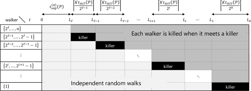
Figure 2: Random walk with a list of allowed killings ([39]).

Formally, define the list of allowed killings $\mathcal{A}=(A_{t})_{t\geq 0}$ as $A_{t}\mathrel{\mathop{:}}=\emptyset$ for $t\leq L_{\ell}$ and $A_{t}\mathrel{\mathop{:}}=\left\{(b,a):2^{i}\leq b<2^{i+1},a\geq 2^{i+1}\right\}$ for $L_{i+1}<t\leq L_{i}$ with $0\leq i<\ell$. Let $Z_{t}(1)=X_{t}(1)$ for all $t\geq 0$. For $t\geq 0$ and $a\geq 1$, $Z_{t}(a)$ is inductively defined as follows. Suppose that $(Z_{s})_{s=0}^{t-1}$ and $Z_{t}(1),\ldots,Z_{t}(a-1)$ are determined. Then, let

$$\tau^{\mathcal{A}}(a) \mathrel{\mathop{:}}=\min\{s\geq 0:\textrm{$X_{s}(a)=Z_{s}(b)$ for some $(b,a)\in A_{s}$}\},\hskip 10.00002pt\mathrm{and}$$

$$Z_{t}(a) \mathrel{\mathop{:}}=\begin{cases}X_{t}(a)&\text{if $t<\tau^{\mathcal{A}}(a)$,}\\ \partial&\text{otherwise}.\end{cases}$$

For a vector $x\in(V\cup\{\partial\})^{n}$, let $\mathcal{S}(x)=\{i\in[n]:x(i)\neq\partial\}$. Obviously, $\mathop{\mathbf{Pr}}[|S(\mathrm{C}_{t})|\geq z|\mathrm{C}_{0}=x]=\mathop{\mathbf{Pr}}[|\mathcal{S}(Y_{t})|\geq z|X_{0}=x]$ holds for any $t\geq 0$, $z\geq 0$ and $x\in V^{n}$. Furthermore, $\mathop{\mathbf{Pr}}[|\mathcal{S}(Y_{t})|\geq z|X_{0}=x]\leq\mathop{\mathbf{Pr}}[|\mathcal{S}(Z_{t})|\geq z|X_{0}=x]$ holds for any $t\geq 0$, $z\geq 0$ and $x\in V^{n}$. To see this, consider using $(\mathrm{C}_{t})_{t\geq 0}$ instead of $(X_{t})_{t\geq 0}$ in definitions of both $(Y_{t})_{t\geq 0}$ and $(Z_{t})_{t\geq 0}$. Then, $|\mathcal{S}(Y_{t})|\leq|\mathcal{S}(Z_{t})|$ holds for any $t\geq 0$. Note that $\mathop{\mathbf{Pr}}[\mathrm{C}_{t}(i)=v|\mathrm{C}_{0}(i)=u]=\mathop{\mathbf{Pr}}[X_{t}(i)=v|X_{0}(i)=u]$ holds for any $u,v\in V$ and $i\in[n]$. From the definition of the random walk with allowed killings, $Z_{t}(i)=X_{t}(i)$ until it meets a killer. Hence, we have

$$\mathop{\mathbf{Pr}}[\tau_{\mathrm{coal}}(\mathcal{P})>L_{0}]$$

$$\leq\mathop{\mathbf{Pr}}\left[|\mathcal{S}(Z_{L_{0}})|\geq 2\right]=\mathop{\mathbf{Pr}}\left[\bigvee_{a=2}^{n}\{\textrm{Walker $a$ is not killed}\}\right]$$

$$=\mathop{\mathbf{Pr}}\left[\bigvee_{a=2}^{n}\bigwedge_{b=1}^{2^{\ell_{a}}-1}\bigwedge_{t=L_{\ell_{b}+1}}^{L_{\ell_{b}}}\{Z_{t}(a)\neq Z_{t}(b)\}\right]=\mathop{\mathbf{Pr}}\left[\bigvee_{a=2}^{n}\bigwedge_{b=1}^{2^{\ell_{a}}-1}\bigwedge_{t=L_{\ell_{b}+1}}^{L_{\ell_{b}}}\{X_{t}(b)\neq X_{t}(a)\}\right].$$

∎

Combining Lemmas 5.3 and 5.1, we obtain the following lemma.

Lemma 5.4.

Let $\mathcal{P}=(P_{t})_{t\geq 1}$ be a sequence of irreducible, reversible, and lazy transition matrices. Suppose that all $P_{t}$ have the same stationary distribution $\pi$. Then, for any $x\in V^{n}$, $\mathop{\mathbf{Pr}}\left[\tau_{\mathrm{coal}}(\mathcal{P})>T\middle|\mathrm{C}_{0}=x\right]\leq 1-10^{-5}$ holds if $T\geq t_{\mathrm{sep}}^{(\pi)}(\mathcal{P})+80t_{\mathrm{hit}}(\mathcal{P})+\log_{2}(n)$.

Proof.

From the definition 2 of the separation time $t_{\mathrm{sep}}^{(\pi)}(\mathcal{P})=L_{\ell}$, there is a transition matrix $Q\in[0,1]^{V\times V}$ such that

$$P_{[1,L_{\ell}]}(x,u)=\frac{1}{2}\pi(u)+\frac{1}{2}Q(x,u)$$

holds for all $x,u\in V$. Hence, the distribution of $n$ walkers $X_{L_{\ell}}(1),\ldots,X_{L_{\ell}}(n)$ can be simulated as follows: Each walker $i\in[n]$ flips its own fair coin. If it is head, the walker’s position $X_{L_{\ell}}(i)$ is sampled according to $\pi$. Otherwise, it is sampled according to the distribution $Q(X_{0}(i),\cdotp)$. Let $I\subseteq[n]$ denote a random subset of indices with a head coin. Let $\mathcal{W}\mathrel{\mathop{:}}=\{W\subseteq[n]:\textrm{$|\{2^{i},\ldots,2^{i+1}-1\}\cap W|\geq 2^{i}/4$ holds for all $0\leq i<\ell$}\}$ be a set of subsets of $[n]$. Then, from Lemma 5.3,

$$\mathop{\mathbf{Pr}}\left[\tau_{\mathrm{coal}}(\mathcal{P})>L_{0}\right]$$

$$\leq\sum_{W\subseteq[n]}\mathop{\mathbf{Pr}}\left[\bigvee_{a=2}^{n}\bigwedge_{b\in[2^{\ell_{a}}-1]}\bigwedge_{t\in[L_{\ell_{b}+1},L_{\ell_{b}}]}\{X_{t}(b)\neq X_{t}(a)\}\middle|I=W\right]\mathop{\mathbf{Pr}}[I=W]$$

$$\leq\mathop{\mathbf{Pr}}[I\notin\mathcal{W}]+\max_{W\in\mathcal{W}}\mathop{\mathbf{Pr}}\left[\bigvee_{a=2}^{n}\bigwedge_{b\in[2^{\ell_{a}}-1]\cap W}\bigwedge_{t\in[L_{\ell_{b}+1},L_{\ell_{b}}]}\{X_{t}(b)\neq X_{t}(a)\}\middle|\bigwedge_{i\in W}\{X_{L_{\ell}}(i)\sim\pi\}\right].$$ (11)

Let $I_{j}=\mathbbm{1}_{j\in I}\in\{0,1\}$ denote the binary indicator for the random subset $I$. For the first term of 11, applying the Chernoff inequality (Lemma C.2) yields

$$\mathop{\mathbf{Pr}}[I\in\mathcal{W}] =\mathop{\mathbf{Pr}}\left[\bigwedge_{i=0}^{\ell-1}\{|I\cap\{2^{i},\ldots,2^{i+1}-1\}|\geq 2^{i}/4\}\right]=\prod_{i=0}^{\ell-1}\mathop{\mathbf{Pr}}\left[\sum_{j=2^{i}}^{2^{i+1}-1}I_{j}\geq 2^{i}/4\right]$$

$$\geq\prod_{i=0}^{5}\left(1-\exp\left(-\frac{2^{i}}{16}\right)\right)\cdot\prod_{i=6}^{\ell-1}\left(1-\exp\left(-\frac{2^{i}}{16}\right)\right)$$

$$\geq 0.00033\cdot\prod_{i=2}^{\ell-5}\left(1-\exp\left(-2^{i}\right)\right)\geq 0.00033\cdot\prod_{i=2}^{\infty}\left(1-2^{-i}\right)$$

$$\geq 0.00033\cdot\left(1-\sum_{i=2}^{\infty}2^{-i}\right)\geq 0.00016.$$ (12)

Note that $\mathop{\mathbf{E}}\left[\sum_{j=2^{i}}^{2^{i+1}-1}I_{j}\right]=2^{i}/2$. Next, we bound the second term of 11. For any $W\in\mathcal{W}$,

$$\mathop{\mathbf{Pr}}\left[\bigvee_{a=2}^{n}\bigwedge_{b\in[2^{\ell_{a}}-1]\cap W}\bigwedge_{t\in[L_{\ell_{b}+1},L_{\ell_{b}}]}\{X_{t}(b)\neq X_{t}(a)\}\middle|\bigwedge_{i\in W}\{X_{L_{\ell}}(i)\sim\pi\}\right]$$

$$\leq\sum_{a=2}^{n}\prod_{b\in[2^{\ell_{a}}-1]\cap W}\mathop{\mathbf{Pr}}\left[\bigwedge_{t\in[L_{\ell_{b}+1},L_{\ell_{b}}]}\{X_{t}(b)\neq X_{t}(a)\}\middle|\bigwedge_{i\in W}\{X_{L_{\ell}}(i)\sim\pi\}\right]$$

holds. Applying the meeting time lemma (Lemma 5.1), for any $b\in W$, we have

$$\mathop{\mathbf{Pr}}\left[\bigwedge_{t\in[L_{\ell_{b}+1},L_{\ell_{b}}]}\{X_{t}(b)\neq X_{t}(a)\}\middle|\bigwedge_{i\in W}\{X_{L_{\ell}}(i)\sim\pi\}\right]\leq\exp\left(-\frac{L_{\ell_{b}}-L_{\ell_{b}+1}}{t_{\mathrm{HIT}}(\mathcal{P})}\right)\leq\exp\left(-\frac{K}{2^{\ell_{b}}}\right).$$

Hence, for any $W\in\mathcal{W}$,

$$\mathop{\mathbf{Pr}}\left[\bigvee_{a=2}^{n}\bigwedge_{b\in[2^{\ell_{a}}-1]\cap W}\bigwedge_{t\in[L_{\ell_{b}+1},L_{\ell_{b}}]}\{X_{t}(b)\neq X_{t}(a)\}\middle|\bigwedge_{i\in W}\{X_{L_{\ell}}(i)\sim\pi\}\right]$$

$$\leq\sum_{i=1}^{\ell-1}\sum_{a=2^{i}}^{2^{i+1}-1}\prod_{j=1}^{i-1}\prod_{b\in\{2^{j},\ldots,2^{j+1}-1\}\cap W}\exp\left(-\frac{K}{2^{j}}\right)\leq\sum_{i=1}^{\ell-1}\sum_{a=2^{i}}^{2^{i+1}-1}\prod_{j=1}^{i-1}\exp\left(-\frac{K}{4}\right)$$

$$\leq\sum_{i=1}^{\ell-1}2^{i}\exp\left(-\frac{K}{4}i\right)\leq\frac{2}{\mathrm{e}^{K/4}-2}.$$ (13)

Combining 11, 12 and 13 with $K=40$, $\mathop{\mathbf{Pr}}\left[\tau_{\mathrm{coal}}(\mathcal{P})>T\middle|\mathrm{C}_{0}=x\right]\leq 1-0.00016+\frac{2}{\mathrm{e}^{10}-2}\leq 1-10^{-5}$ holds. ∎

Proof of Theorem 5.2.

Let $T\mathrel{\mathop{:}}=\lceil(85+o_{n}(1))t_{\mathrm{HIT}}(\mathcal{P})\rceil$. Lemma 5.4 implies that, for any $t\geq 0$ and $x\in V^{n}$, $\mathop{\mathbf{Pr}}[\tau_{\mathrm{coal}}(\mathcal{P})>t+T|\mathrm{C}_{t}=x]\leq 1-10^{-5}$ holds. Thus we obtain the claim from Corollary B.2. ∎

5.3 Lower bound of meeting time

In this section, we prove Proposition 1.5.

Proof of Proposition 1.5.

We consider the lazy simple random walk on the graph sequence given in Proposition 12 of [41]. For completeness, we present the sequence formally. For a graph $H$ and a permutation $\eta$ on $V(H)$, let $\eta(H)$ be the graph given by $V(\eta(H))=V(H)$ and $E(\eta(H))=\{\{\eta(u),\eta(v)\}:\{u,v\}\in E(H)\}$.

For any integer $m\in\mathbb{N}$, let $U=\{u_{0},\dots,u_{m-1}\}$ and $W=\{w_{0},\dots,w_{m-1}\}$. Define the graph $G$ by $V(G)\mathrel{\mathop{:}}=U\cup W$ and

$$E(G)\mathrel{\mathop{:}}=\{u_{0},w_{0}\}\cup\bigcup_{i=1}^{m-1}\{u_{i},u_{0}\}\cup\bigcup_{j=1}^{m-1}\{w_{j},w_{0}\}.$$ (14)

Let $\eta$ be the permutation on $V$ defined by $\eta(u_{i})=u_{(i+1)\bmod m}$ and $\eta(w_{i})=w_{(i+1)\bmod m}$.

Figure 3: The graph $G$ given by 14 for $m=4$ (left) and $\eta(G)$ (right).

We claim that the lazy simple random walk on the sequence $(G_{t})_{t\geq 1}$ given by $G_{1}=G$ and $G_{t+1}=\eta(G_{t})$ ($t\geq 1$) has the desired property (see Figure 3). Consider two independent lazy simple random walks $(X_{t}(1))_{t\geq 0}$ and $(X_{t}(2))_{t\geq 0}$ with initial positions $(X_{0}(1),X_{0}(2))=(u_{m-1},w_{m-1})$. Suppose $\tau_{\mathrm{meet}}\leq t$. Then, there exists $t^{\prime}\leq t$ such that either $X(1)$ or $X(2)$ moves along the edge $\{u_{j},w_{j}\}$ for $j=t^{\prime}\bmod m$. Focus on the walk $X(1)$ and suppose $X_{t^{\prime}-1}(1)\in U$ and $X_{t^{\prime}}(1)\in W$. To reach $u_{j}$, the walker $X(1)$ must choose the self loop for $m-1$ consecutive times, which occurs with probability $2^{-m+1}$. Therefore, by the union bound over $X(0)$ and $X(1)$, we have $\mathop{\mathbf{Pr}}[\tau_{\mathrm{meet}}\leq t]\leq 2\cdot 2^{-m+1}$ and we have $t_{\mathrm{meet}}=2^{\Omega(m)}$. ∎

6 Pull voting

In this section, we prove Theorem 1.8. Our proof of bounding $\mathop{\mathbf{E}}[\tau_{\mathrm{cons}}]$ is inspired by the idea of well-known duality between the pull voting and coalescing random walk [26].

Proposition 6.1 (Duality in static setting [26]).

Let $P\in[0,1]^{V\times V}$ be an irreducible transition matrix. Let $\tau_{\mathrm{cons}}(P)$ be the consensus time of the pull voting according to $P$ where all vertices initially hold distinct opinions. Let $\tau_{\mathrm{coal}}(P)$ be the coalescing time of the coalescing random walk according to $P$. Then, for every $j\geq 0$, $\mathop{\mathbf{Pr}}[\tau_{\mathrm{coal}}(P)\leq j]=\mathop{\mathbf{Pr}}[\tau_{\mathrm{cons}}(P)\leq j]$ holds.

From Proposition 6.1, we can obtain bounds of $\tau_{\mathrm{cons}}$ by studying $\tau_{\mathrm{coal}}$. Indeed, the proof of previous results bounding $\tau_{\mathrm{cons}}$ on a static graph relies on the duality. In this paper, we obtain the following consensus–coalescing relation that is analogous to Proposition 6.1 in the time inhomogeneous setting.

Proposition 6.2 (Consensus–Coalescing relation on dynamic graphs).

Let $\mathcal{P}$ be a sequence of transition matrices (not necessarily has a time-homogeneous stationary distribution). Consider the pull voting according to $\mathcal{P}$ such that initially all vertices have $n$ distinct opinions. Then, there is a sequence $(\mathcal{Q}^{(i)})_{i\geq 0}$ where each $\mathcal{Q}^{(i)}=(Q^{(i)}_{t})_{t\geq 1}$ is a transition matrix sequence such that, for every $j\geq 0$,

$$\mathop{\mathbf{Pr}}[\tau_{\mathrm{cons}}(\mathcal{P})\leq j]=\mathop{\mathbf{Pr}}[\tau_{\mathrm{coal}}(\mathcal{Q}^{(j)})\leq j]$$

holds. Moreover, if $\mathcal{P}$ is reversible and has the time-invariant stationary distribution $\pi$, then so do the sequences $\mathcal{Q}^{(i)}$ for all $i$.

Indeed, if $\mathcal{P}=(P)_{t\geq 1}$ is a sequence of a static transition matrix, then $\mathcal{Q}^{(i)}=\mathcal{P}$ for all $i\geq 0$, implying Proposition 6.1.

The proof of the duality theorem in the static setting (Proposition 6.1) is obtained by constructing a coupling of the pull voting and the coalescing random walk with equal consensus and coalescing times. Our proof of Proposition 6.2 is based on essentially the same argument. In Section 6.4, we present a sequence of graphs on which the pull voting according to $P_{\mathrm{LS}}$ on it has an exponential consensus time as follows:

Proposition 6.3.

There is a sequence $(G_{t})_{t\geq 1}$ of graphs on which the pull voting according to $\mathcal{P}=(P_{\mathrm{LS}}(G_{t}))_{t\geq 1}$ over opinion set $\Sigma=\{0,1\}$ satisfies $t_{\mathrm{cons}}=2^{\Omega(n)}$.

6.1 Consensus–Coalescing relation

We prove Proposition 6.2. The proof is essentially based on the notion of linear voter model of [17].

Proof of Proposition 6.2..

Let $P\in[0,1]^{V\times V}$ be a transition matrix and $\mathcal{S}$ be the set of all binary $V\times V$ matrices such that each row contains exactly one $1$. For each matrix $S\in\mathcal{S}$, we define a probability distribution $\mu_{P}$ over $\mathcal{S}$ by

$$\mu_{P}(S)=\prod_{(i,j)\in V\times V:S_{i,j}=1}P_{i,j}$$

for each $S\in\mathcal{S}$. We interpret $S\in\mathcal{S}$ as the list of selections at a specific round of the pull voting: Specifically, $s_{i,j}=1$ if and only if $i$ selects $j$ at the pull voting. Then, $\mu_{P}(\cdot)$ can be seen as the probability distribution over the set of all possible selection lists during the pull voting according to $P$.

Given a sequence $S_{1},\dots,S_{i}\in\mathcal{S}$ of $i$ matrices, we can simulate the pull voting for $i$ rounds as follows. Let $y_{0}\in\Sigma^{V}$ denote the initial opinion configuration where each vertex has a distinct opinion. Then, $y_{i}=S_{i}y_{i-1}=S_{i}S_{i-1}\dots S_{1}y_{0}=\prod_{t=1}^{i}S_{i-t+1}y_{0}$. We say that an opinion vector $y\in\Sigma^{V}$ is in consensus if $y=\sigma\mathbbm{1}$ holds for some $\sigma\in\Sigma$. For fixed $i\in\mathbb{N}$, let

$$\mathcal{S}^{(i)}_{\mathrm{cons}}=\{(S_{1},\dots,S_{i})\in\mathcal{S}^{i}:\text{$y_{i}$ is in consensus}\}.$$

Here, note that, if $y_{i-1}$ is in consensus, then so does $y_{i}=S_{i}y_{i-1}$. Then, we have

$$\mathop{\mathbf{Pr}}[\tau_{\mathrm{cons}}(\mathcal{P})\leq i]=\sum_{(S_{1},\dots,S_{i})\in\mathcal{S}^{(i)}_{\mathrm{cons}}}\prod_{t=1}^{i}\mu_{P_{t}}(S_{t}).$$ (15)

We show that, for every $i$, there is a sequence $\mathcal{Q}=\mathcal{Q}^{(i)}=(Q^{(i)}_{t})_{t\geq 0}$ of transition matrices such that the right hand side of 15 is equal to $\mathop{\mathbf{Pr}}[\tau_{\mathrm{coal}}(\mathcal{Q}^{(i)})\leq i]$. Consider the sequence $\mathcal{Q}^{(i)}$ defined by

$$Q^{(i)}_{t}=\begin{cases}P_{i-t+1}&\text{if $t\leq i$},\\ P_{0}&\text{if $t>i$}.\end{cases}$$

Note that, if $\mathcal{P}$ is reversible and has a time-invariant stationary distribution $\pi$, then so does $\mathcal{Q}^{(i)}$ for every $i$.

Fix $i$ and consider the coalescing random walk according to $\mathcal{Q}^{(i)}$. We call a vector $c\in\mathbb{Z}_{\geq 0}^{V}$ satisfying $\sum_{v\in V}c_{i}=|V|$ a walker configuration vector. A walker configuration vector can be interpreted as the vector denoting the number of walkers on vertices, i.e., $c_{v}$ is the number of walkers on $v$. Given $S^{\prime}_{1},\dots,S^{\prime}_{i}\in\mathcal{S}$, we can simulate the coalescing random walk for $i$ rounds as follows: Let $c_{0}=\mathbbm{1}^{\top}$ (initially, each vertices has exactly one walker). For $1\leq j\leq i$, let $c_{j}=c_{j-1}S^{\prime}_{j}=c_{0}\prod_{k=1}^{j}S^{\prime}_{k}$. Intuitively speaking, the matrix $S^{\prime}_{j}$ denotes the transition result: $(S^{\prime}_{j})_{u,v}=1$ if and only if $u$ sends all walkers on it to $v$ at the $j$-th round. A vertex $v\in V$ at round $i$ has a walker if and only if $(c_{i})_{v}>0$.

We say that a walker configuration vector $c$ is in coalesce if $c=|V|e_{v}$ for some $v\in V$, where $e_{v}\in\{0,1\}^{V}$ is the binary indicator vector for a vertex $v$ (i.e., $(e_{v})_{u}=1$ if and only if $v=u$). Note that, if $c_{j-1}$ is in coalesce, then so does $c_{j}=c_{j-1}S^{\prime}_{j}$. For a coalescing random walk is according to a transition matrix $Q$, a transition result $S^{\prime}\in\mathcal{S}$ occurs with probability $\mu_{Q}(S^{\prime})$. Let

$$\mathcal{S}^{(i)}_{\mathrm{coal}}=\{(S^{\prime}_{1},\dots,S^{\prime}_{i})\in\mathcal{S}^{i}:\text{$c_{i}$ is coalescing}\}.$$

Then, we have

$$\mathop{\mathbf{Pr}}[\tau_{\mathrm{coal}}(\mathcal{Q}^{(i)})\leq i]=\sum_{(S^{\prime}_{1},\dots,S^{\prime}_{i})\in\mathcal{S}^{(i)}_{\mathrm{coal}}}\prod_{t=1}^{i}\mu_{Q^{(i)}_{t}}(S^{\prime}_{t})=\sum_{(S^{\prime}_{1},\dots,S^{\prime}_{i})\in\mathcal{S}^{(i)}_{\mathrm{coal}}}\prod_{t=1}^{i}\mu_{P_{t}}(S^{\prime}_{i-t+1}).$$ (16)

We compare 15 and 16. Indeed, it holds that $(S_{1},\dots,S_{i})\in\mathcal{S}^{(i)}_{\mathrm{cons}}$ if and only if $(S_{i},\dots,S_{1})\in\mathcal{S}^{(i)}_{\mathrm{coal}}$. To see this, suppose $(S_{1},\dots,S_{i})\in\mathcal{S}^{(i)}_{\mathrm{cons}}$. Then, the opinion configuration vector $y_{i}$ at the $i$-th round satisfies $y_{i}=S_{i}\dots S_{1}y_{0}=\sigma_{w}\mathbbm{1}$ for some $w\in V$, where $\sigma_{w}\in\Sigma$ is the opinion that $w\in V$ initially holds. Since this relation holds regardless of the labels $\Sigma$ of opinions, we have $S_{i}\dots S_{1}e_{w}=\mathbbm{1}$ and $S_{i}\dots S_{1}e_{v}=\mathbf{0}$ for $v\neq w$, where $\mathbf{0}$ denotes the all-zero vector. Therefore,

$$\mathbbm{1}^{\top}S_{i}S_{i-1}\dots S_{1}e_{v} =\begin{cases}|V|&\text{if $v=w$},\\ 0&\text{otherwise}\end{cases}$$

and thus $\mathbbm{1}^{\top}\prod_{t=1}^{i}S_{i-t+1}=|V|e_{w}^{\top}$. In other words, $(S^{\prime}_{1},\dots,S^{\prime}_{i})\mathrel{\mathop{:}}=(S_{i},\dots,S_{1})\in\mathcal{S}^{(i)}_{\mathrm{coal}}$. The converse direction (i.e., $(S^{\prime}_{1},\dots,S^{\prime}_{i})\in\mathcal{S}^{(i)}_{\mathrm{coal}}$ implies $(S^{\prime}_{i},\dots,S^{\prime}_{1})\in\mathcal{S}^{(i)}_{\mathrm{cons}}$) can be checked similarly: If $(S^{\prime}_{1},\dots,S^{\prime}_{i})\in\mathcal{S}^{(i)}_{\mathrm{coal}}$, then $\mathbbm{1}^{\top}S^{\prime}_{1}\dots S^{\prime}_{i}=|V|e_{w}^{\top}$ for some $w\in V$. Then, for $(S_{1},\dots,S_{i})\mathrel{\mathop{:}}=(S^{\prime}_{i},\dots,S^{\prime}_{1})$, we have $\mathbbm{1}^{\top}S_{i}\cdots S_{1}e_{w}=\mathbbm{1}^{\top}S^{\prime}_{1}\cdots S^{\prime}_{i}e_{w}=|V|$. Since $\mathbf{0}\leq S_{i}\cdots S_{1}e_{w}\leq S_{i}\cdots S_{1}\mathbbm{1}=\mathbbm{1}$ (here, we write $(x_{1},\dots,x_{n})\leq(y_{1},\dots,y_{n})$ if $x_{i}\leq y_{i}$ for all $i\in[n]$), we have $S_{i}\cdots S_{1}e_{w}=\mathbbm{1}$. This implies $(S_{1},\dots,S_{i})\in\mathcal{S}^{(i)}_{\mathrm{cons}}$.

The mapping $\phi\colon(S_{1},\dots,S_{i})\mapsto(S_{i},\dots,S_{1})$ is a bijection between $\mathcal{S}^{(i)}_{\mathrm{cons}}$ and $\mathcal{S}^{(i)}_{\mathrm{coal}}$ preserving the product measure $\prod_{t=1}^{i}\mu_{P}(S_{t})$. This implies that 15 and 16 are equal, completing the proof of Proposition 6.2. ∎

6.2 Consensus time

Proof of Theorem 1.8.

If $\mathcal{P}$ is irreducible, lazy, and reversible with respect to $\pi\in(0,1]^{V}$, so does $\mathcal{Q}^{(i)}$ for all $i\geq 0$. Therefore, from Theorem 5.2, $\mathop{\mathbf{E}}[\tau_{\mathrm{coal}}(\mathcal{Q}^{(i)}]\leq T$ for all $i$, where $T=C\cdot t_{\mathrm{HIT}}(\mathcal{P})$ for some absolute constant $C>0$. Then, from Proposition 6.2, we have

$$\mathop{\mathbf{Pr}}[\tau_{\mathrm{cons}}(\mathcal{P})\geq 2T]=\mathop{\mathbf{Pr}}[\tau_{\mathrm{coal}}(\mathcal{Q}^{(2T)})\geq 2T]\leq\frac{\mathop{\mathbf{E}}[\tau_{\mathrm{coal}}(\mathcal{Q}^{(2T)})]}{2T}\leq\frac{1}{2}.$$

Here, the initial opinion configuration is the worst one that all vertices have $n$ distinct opinions. Therefore, for any fixed $t\geq 0$, $\mathop{\mathbf{Pr}}[\tau_{\mathrm{cons}}((P_{t+s})_{s\geq 0})>2T]\leq 1/2$ holds for any initial opinion configuration. From Corollary B.2 we have $\mathop{\mathbf{E}}[\tau_{\mathrm{cons}}(\mathcal{P})]\leq 4T=4Ct_{\mathrm{HIT}}(\mathcal{P})=O(t_{\mathrm{HIT}}(\mathcal{P}))$. ∎

6.3 Winning probability

We prove Proposition 1.10. Our proof is based on the voting martingale argument that was used to obtain the winning probability result for the static graph setting (cf. [26, 17]). We just verify that the argument works for our dynamic graph setting. For completeness, we write the proof in this subsection.

Proof of Proposition 1.10..

We first consider the special case of $\Sigma=\{0,1\}$ and then go on to the general case $\Sigma\subseteq\{0,\dots,n-1\}$.

The case of $\Sigma=\{0,1\}$.

Let $(Y_{t})_{t\geq 0}$ be the pull voting according to $\mathcal{P}=(P_{t})_{t\geq 1}$ with a time-homogeneous stationary distribution $\pi$. Note that $Y_{t}\in\{0,1\}^{V}$. In this proof, we promise that $Y_{t}$ is an $n\times 1$ vector and $\pi\in[0,1]^{V}$ is a $1\times n$ vector. Let $\pi(Y_{t})=\sum_{u\in V}\pi(u)Y_{t}(u)$. We first claim that $(\pi(Y_{t}))_{t\geq 0}$ is a martingale with respect to $Y_{t}$. To see this, observe

$$\mathop{\mathbf{E}}[\pi(Y_{t+1})|Y_{t}] =\sum_{u\in V}\pi(u)\mathop{\mathbf{Pr}}[Y_{t+1}(u)=1|Y_{t}]=\sum_{u\in V}\pi(u)\sum_{w\in V}(P_{t})(u,w)Y_{t}(w)$$

$$=\sum_{w\in V}(\pi P_{t})(w)Y_{t}(w)=\sum_{w\in V}\pi(w)Y_{t}(w)=\pi(Y_{t}).$$

Since $\pi(Y_{t})$ are bounded, we can apply the Optimal Stopping Theorem and obtain $\mathop{\mathbf{E}}[\pi(Y_{\tau_{\mathrm{cons}}})]=\pi(Y_{0})$. Note that, since $Y_{\tau_{\mathrm{cons}}}$ is either all-zero or all-one, we have

$$\mathop{\mathbf{E}}[\pi(Y_{\tau_{\mathrm{cons}}})] =\pi(\mathbbm{1})\mathop{\mathbf{Pr}}[Y_{\tau_{\mathrm{cons}}}=\mathbbm{1}]=\mathop{\mathbf{Pr}}[Y_{\tau_{\mathrm{cons}}}=\mathbbm{1}].$$

In other words, the probability that the opinion $1$ wins is equal to $\pi(Y_{0})=\sum_{v\in V:Y_{0}(v)=1}\pi(v)$.

General case.

We reduce the general case to the binary opinion case by regarding $\sigma=1$ for a fixed opinion $\sigma\in\Sigma$ and all other opinions are zero. Then we obtain the claim from the argument for the binary opinion case. ∎

6.4 Exponential consensus time

In this subsection, we prove Proposition 6.3. Consider the graph $G=(U\cup W,E)$ and permutation $\eta\colon V(G)\to V(G)$ defined in Section 5.3. Suppose vertices in $U$ have opinion $0$ and that in $W$ have opinion $1$ initially. We claim that the sequence $(G_{t})_{t\geq 1}$ given by $G_{1}=G$ and $G_{t}=\eta(G_{t-1})$ with the initial opinion configuration above has the exponential consensus time.

By the monotonicity of the pull voting, we consider the following setting. Suppose only vertices in $U=\{u_{0},\dots,u_{m-1}\}$ perform the pull voting and vertices in $W$ always have opinion $1$. Let $\tau$ be the time to reach the opinion configuration where all vertices in $U$ have opinion $1$. It suffices to prove $\mathop{\mathbf{E}}[\tau]=2^{\Omega(m)}$, where $|U|=m$.

Since the graph dynamics is given by the iteration of applying the permutation $\eta$, it is convenient to consider the following equivalent process: At the $t$-th round, vertices perform the one-round pull voting and then opinions are shuffled according to $\eta$. That is, if $Y_{t-1}\in\{0,1\}^{U}$ denote the opinion configuration at the beginning of the $t$-th round, we first update $Y_{t-1}$ by the pull voting to obtain $Z_{t}\in\{0,1\}^{U}$ and then set $Y_{t}(\eta(u))=Z_{t}(u)$ for every $u\in U$. Note that the permutation $\eta$ defined in Section 5.3 satisfies $\eta(U)=U$. We consider the sequence $(Y_{t})_{t\geq 0}$ described above, where $Y_{0}$ is the all-zero vector. Note that the process agrees with the opinion $1$ at the last of the $t$-th round if and only if $Y_{t}(u)=1$ for all $u\in U$.

Let $\tau^{\prime}=\inf\{t\geq 0\colon Y_{t}(0)=1\}$. Then, for any $i=1,\dots,m-1$, the vertex $u_{i}$ must choose the self-loop in the pull voting procedure at the $(\tau^{\prime}-i)$-th round to keep $u_{i}$’s opinion $1$ (otherwise, $u_{i}$ selects $u_{0}$, who has opinion $0$). This happens with probability $2^{-m+1}$ and therefore we have $\mathop{\mathbf{E}}[\tau]\geq\mathop{\mathbf{E}}[\tau^{\prime}]=2^{\Omega(m)}$. This completes the proof of Proposition 6.3.

7 Metropolis walk on edge-Markovian graph

In this section, we prove Theorem 1.7. Let $V$ be a vertex set with $|V|=n$ and $p,q\in[0,1]$ be two parameters. Let $\left((Y_{t}(e))_{t\geq 0}\right)_{e\in\binom{V}{2}}$ be $\binom{n}{2}$ independent Markov chains, where each $(Y_{t}(e))_{t\geq 0}$ is the Markov chain with the state space $\{0,1\}$ and the transition matrix $M=M_{p,q}\mathrel{\mathop{:}}=\left(\begin{array}[]{cc}1-p&p\\ q&1-q\end{array}\right)$. Henceforth, write $Y_{t}=(Y_{t}(e))_{e\in\binom{V}{2}}$ for convenience. The edge-Markovian graph $\mathcal{G}(n,p,q)$ is a sequence of random graphs $(G_{t})_{t\geq 0}=((V,E_{t}))_{t\geq 0}$, where $E_{t}\mathrel{\mathop{:}}=\left\{e\in\binom{V}{2}:Y_{t}(e)=1\right\}$ for all $t\geq 0$. We show the following lemma in this section.

Lemma 7.1.

Suppose that $0<p+q\leq 1$ and $\frac{p}{p+q}\geq 32(c+1)\frac{\log n}{n}$ hold for an arbitrary $c>0$. Let $\mathcal{G}(n,p,q)=(G_{t})_{t\geq 0}$ be the edge-Markovian graph. Let $I=I(p,q)\mathrel{\mathop{:}}=\left\lceil\frac{\max\{1,\log(q/p)\}}{p+q}\right\rceil$ and $J\leq n^{c}/2$. For any $\ell\geq 0$ and $0\leq i\leq\ell$, let $S(\ell,i)\mathrel{\mathop{:}}=\left(\frac{\ell(\ell-1)}{2}+i\right)(I+J)=\left(\sum_{j=1}^{\ell-1}j+i\right)(I+J)$. Let $C=8192$. Then, for any $Y_{0}=b\in\{0,1\}^{\binom{V}{2}}$,

$$\mathop{\mathbf{Pr}}\left[\bigwedge_{\ell=1}^{\infty}\bigvee_{i=1}^{\ell}\left\{t_{\mathrm{REL}}\left(\left(P_{\mathrm{LM}}(G_{t})\right)_{t=S(\ell,i-1)+I}^{S(\ell,i)}\right)\leq C\right\}\right]\geq 1-\frac{1}{n}.$$

Proof.

For $S\subseteq V$, let $Q_{t}(S)=\sum_{u\in S}\sum_{v\notin S}\pi(u)P_{t}(u,v)$ and $\pi(S)=\sum_{v\in S}\pi(v)$. Let $C_{t}(S)=\sum_{u\in S}\sum_{v\notin S}Y_{t}(\{u,v\})$. From 3, we have

$$\frac{Q_{t}(S)}{\pi(S)} =\frac{n}{|S|}\sum_{u\in S}\sum_{v\notin S}\frac{1}{n}\frac{Y_{t}(\{u,v\})}{2\max\{\deg(G_{t},u),\deg(G_{t},v)\}}\geq\frac{C_{t}(S)}{2|S|d_{\max}(G_{t})}.$$ (17)

Now, it is easy to check that

$$M^{t}=\frac{1}{p+q}\left[\left(\begin{array}[]{cc}q&p\\ q&p\end{array}\right)+(1-p-q)^{t}\left(\begin{array}[]{cc}p&-p\\ -q&q\end{array}\right)\right]$$

holds for any $t\geq 1$. Hence, for any $e\in\binom{V}{2}$, $s\geq 0$, $I^{\prime}\geq I=\left\lceil\frac{\max\{1,\log(q/p)\}}{p+q}\right\rceil$ and $b\in\{0,1\}$, $\mathop{\mathbf{Pr}}[Y_{s+I^{\prime}}(e)=1|Y_{s}(e)=b]=M^{I^{\prime}}(b,1)$ and

$$\frac{p}{2(p+q)}\leq\frac{p}{p+q}\left(1-(1-p-q)^{I^{\prime}}\right)\leq M^{I^{\prime}}(b,1)\leq\frac{p}{p+q}\left(1+(1-p-q)^{I^{\prime}}\frac{q}{p}\right)\leq\frac{2p}{p+q}.$$ (18)

Using 18 and the Chernoff inequality (Lemma C.2), for any $s\geq 0$, $I^{\prime}\geq I$ and $b\in\{0,1\}^{\binom{V}{2}}$, we have

$$\mathop{\mathbf{Pr}}\left[\bigvee_{S\subseteq V:1\leq|S|\leq n/2}\left\{C_{s+I^{\prime}}(S)\leq\frac{1}{2}\frac{|S|np}{4(p+q)}\right\}\middle|Y_{s}=b\right]$$

$$\leq\sum_{S\subseteq V:1\leq|S|\leq n/2}\exp\left(-\frac{|S|np}{32(p+q)}\right)\leq\sum_{S\subseteq V:1\leq|S|\leq n/2}\exp\left(-(c+1)|S|\log n\right)$$

$$=\sum_{1\leq x\leq n/2}\binom{n}{x}\frac{1}{n^{(c+1)x}}\leq\frac{1}{n^{c}-1}.$$ (19)

Note that $\mathop{\mathbf{E}}\left[C_{s+I^{\prime}}(S)\middle|Y_{s}=b\right]\geq|S|(n-|S|)\frac{p}{2(p+q)}\geq\frac{|S|np}{4(p+q)}$ for any $1\leq|S|\leq n/2$. Furthermore, since $\mathop{\mathbf{E}}\left[\deg(G_{s+I^{\prime}},v)\middle|Y_{s}=b\right]\leq n\frac{2p}{p+q}$, we have

$$\mathop{\mathbf{Pr}}\left[\bigvee_{v\in V}\left\{\deg(G_{t},v)\geq 2n\frac{2p}{p+q}\right\}\middle|Y_{s}=b\right]\leq\sum_{v\in V}\exp\left(-\frac{2np}{3(p+q)}\right)\leq\frac{1}{n^{64(c+1)/3-1}}.$$ (20)

Combining 17, 19 and 20, it holds with probability at least $1-\frac{2}{n^{c}}$ that

$$\min_{S\subseteq V:0<\pi(S)\leq 1/2}\frac{Q_{s+I^{\prime}}(S)}{\pi(S)} \geq\frac{|S|np}{8(p+q)}\frac{p+q}{2|S|4np}=\frac{1}{64}.$$

Hence, applying Lemma C.3 yields the following: For any $s\geq 0$, $I^{\prime}\geq I$ and $b\in\{0,1\}^{\binom{V}{2}}$,

$$\mathop{\mathbf{Pr}}\left[t_{\mathrm{rel}}\left(P_{\mathrm{LM}}(G_{s+I^{\prime}})\right)\leq C\middle|Y_{s}=b\right]\geq 1-\frac{2}{n^{c}}.$$ (21)

Here, $C=2\cdotp 64^{2}=8192$.

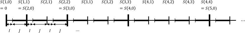
Figure 4: Parameters defined in Lemma 7.1.

From 21 and the union bound,

$$\mathop{\mathbf{Pr}}\left[t_{\mathrm{REL}}\left((P_{\mathrm{LM}}(G_{t}))_{t=s+I}^{s+I+J}\right)>C\middle|Y_{s}=b\right]=\mathop{\mathbf{Pr}}\left[\bigvee_{t=s+I}^{s+I+J}\left\{t_{\mathrm{rel}}\left(P_{\mathrm{LM}}(G_{t})\right)>C\right\}\middle|Y_{s}=b\right]\leq\frac{2J}{n^{c}}\leq\frac{1}{n}$$ (22)

holds for any $s\geq 0$. Let $\mathcal{E}_{i}^{(\ell)}$ be the event that $t_{\mathrm{REL}}\left((P_{\mathrm{LM}}(G_{t}))_{t=S(\ell,i-1)+I}^{S(\ell,i)}\right)>C$. Fix $Y_{0}=b$. From 22, we have

$$\mathop{\mathbf{Pr}}\left[\bigwedge_{i=1}^{\ell}\mathcal{E}_{i}^{(\ell)}\right] =\sum_{b^{\prime}\in\{0,1\}^{\binom{V}{2}}}\mathop{\mathbf{Pr}}\left[\mathcal{E}_{\ell}^{(\ell)}\middle|\bigwedge_{i=1}^{\ell-1}\mathcal{E}_{i}^{(\ell)},Y_{S(\ell,\ell-1)}=b^{\prime}\right]\mathop{\mathbf{Pr}}\left[\bigwedge_{i=1}^{\ell-1}\mathcal{E}_{i}^{(\ell)},Y_{S(\ell,\ell-1)}=b^{\prime}\right]$$

$$\leq\frac{1}{n}\mathop{\mathbf{Pr}}\left[\bigwedge_{i=1}^{\ell-1}\mathcal{E}_{i}^{(\ell)}\right]\leq\cdots\leq\frac{1}{n^{\ell}}.$$

Hence, we obtain

$$\mathop{\mathbf{Pr}}\left[\bigwedge_{\ell=1}^{\infty}\bigvee_{i=1}^{\ell}\overline{\mathcal{E}_{\ell}^{(i)}}\right] =1-\mathop{\mathbf{Pr}}\left[\bigvee_{\ell=1}^{\infty}\bigwedge_{i=1}^{\ell}\mathcal{E}_{\ell}^{(i)}\right]\geq 1-\sum_{\ell=1}^{\infty}\mathop{\mathbf{Pr}}\left[\bigwedge_{i=1}^{\ell}\mathcal{E}_{\ell}^{(i)}\right]\geq 1-\sum_{\ell=1}^{\infty}\frac{1}{n^{\ell}}.$$

∎

Proof of the hitting time bound in Theorem 1.7.

Let $J=\lceil 8192(2\log n+\log 2)+20\cdotp 8192n/k\rceil$. From Lemmas 7.1 and 4.4, it holds for any $\ell\geq 1$ that $\mathop{\mathbf{Pr}}[\tau_{\mathrm{hit}}^{(k)}(\mathcal{P})>S(\ell+1,0)|\tau_{\mathrm{hit}}^{(k)}(\mathcal{P})>S(\ell,0)]\leq 0.9$. Applying Lemma B.3 yields $\mathop{\mathbf{E}}[\tau_{\mathrm{hit}}^{(k)}(\mathcal{P})]\leq\sum_{\ell=0}^{\infty}\ell(I+J)(0.9)^{\ell}\leq 100(I+J)$. ∎

Proof of the cover time bound in Theorem 1.7.

Let $J=\lceil 8192(2\log n+\log 2)+20\cdotp 8192n\log n/k\rceil$. From Lemmas 7.1 and 4.5, it holds for any $\ell\geq 1$ that $\mathop{\mathbf{Pr}}[\tau_{\mathrm{cov}}^{(k)}>S(\ell+1,0)|\tau_{\mathrm{cov}}^{(k)}>S(\ell,0)]\leq 0.9$. Applying Lemma B.3, $\mathop{\mathbf{E}}[\tau_{\mathrm{cov}}^{(k)}(\mathcal{P})]\leq\sum_{\ell=0}^{\infty}\ell(I+J)(0.9)^{\ell}\leq 100(I+J)$ holds. ∎

Proof of the coalescing time bound in Theorem 1.7.

Let $J=\lceil 8192Cn\rceil$. From Lemmas 7.1 and 5.4, it holds for any $\ell\geq 1$ that $\mathop{\mathbf{Pr}}[\tau_{\mathrm{coal}}(\mathcal{P})>S(\ell+1,0)|\tau_{\mathrm{coal}}(\mathcal{P})>S(\ell,0)]\leq 1-10^{-5}$ for any $\ell$. Applying Lemma B.3, $\mathop{\mathbf{E}}[\tau_{\mathrm{coal}}(\mathcal{P})]\leq\sum_{\ell=0}^{\infty}\ell(I+J)(1-10^{-5})^{\ell}\leq C^{\prime}(I+J)$ holds for some absolute constant $C^{\prime}>0$. ∎

8 Conclusion

We obtain new bounds of the mixing, hitting, and cover times of the random walk according to the sequence of irreducible, reversible, and lazy transition matrices that have the same stationary distribution. These bounds generalize previous works for a lazy simple random walk or a $d_{\max}$-lazy walk and improve them in various cases. Furthermore, we obtain the first bounds of the hitting and cover times of multiple random walks and the coalescing time on dynamic graphs. Additionally, we bound the consensus time of the pull-voting on dynamic graphs. Our results strengthen the observation that time inhomogeneous Markov chains with an invariant stationary distribution behaves almost identically to a time-homogeneous chain. Specifically, we prove that if all $P_{t}$ have the same stationary distribution, then $t_{\mathrm{hit}}\left((P_{t})_{t\geq 1}\right)\leq O\left(\max_{t\geq 1}t_{\mathrm{hit}}(P_{t})\right)$ holds (Theorem 1.4). It is natural to ask for the same relation for other parameters. For example, does $t_{\mathrm{cov}}(\mathcal{P})\leq O\left(\max_{t\geq 1}t_{\mathrm{cov}}(P_{t})\right)$ hold?

Most previous works on time-inhomogeneous random walks have translated techniques from time-homogeneous chains into time-inhomogeneous ones: In particular, several known upper bounds (including ours) are based on spectral arguments, which essentially requires the time-homogeneity of the stationary distribution. On the other hand, known lower bounds such as the Sisyphus wheel are based on some combinatorial arguments. To understand time-inhomogeneous random walks with time-varying stationary distributions, it might be important to interpolate the spectral and combinatorial arguments. The simple random walk on any static connected graph has an $O(n^{3})$ cover time. This research question might be a possible future direction of the research of time-inhomogeneous chains.

Appendix A Tools for key lemmas

In this section, we introduce technical tools for Lemmas 3.3, 3.2, 5.1 and 4.3. The first one is concerned with the spectral radius $\rho(D_{w}PD_{w})$ of the substochastic matrix $D_{w}PD_{w}$ (see Section 1.4 for the definition of $D_{w}$). It is known that $\rho(D_{w}PD_{w})\leq 1-1/t_{\mathrm{hit}}(P)$ for any irreducible $D_{w}PD_{w}$ (Section 3.6.5 of [2]). For completeness, we show this under the assumption of irreducibility and reversibility of $P$ as follows.

Lemma A.1.

Let $P\in[0,1]^{V\times V}$ be an irreducible and reversible transition matrix. Then, for any $w\in V$,

$$\rho\left(D_{w}PD_{w}\right)\leq 1-\frac{1}{t_{\mathrm{hit}}(P)}.$$

Proof.

Define $P_{w}\in[0,1]^{V\setminus\{w\}\times V\setminus\{w\}}$ by $P_{w}(u,v)=P(u,v)$ for any $u,v\in V\setminus\{w\}$. The Perron–Frobenius theorem implies that $\lambda=\rho(P_{w})$ is an eigenvalue of $P_{w}$ and there is a nonnegative nonzero eigenvector $g\in\mathbbm{R}^{V\setminus\{w\}}$ satisfying $P_{w}g=\lambda g$ (see, e.g., Theorem 8.3.1 in [27]). Write $Q_{w}=D_{w}PD_{w}$ for convenience. Define $h\in\mathbbm{R}^{V}$ by $h(w)=0$ and $h(v)=\frac{g(v)\pi(v)}{Z}$ for any $v\in V\setminus\{w\}$, where $Z=\sum_{v\in V\setminus\{w\}}g(v)\pi(v)$. Then, $h$ is a probability vector. Furthermore,

$$(hQ_{w})(v) =\sum_{u\in V}h(u)Q_{w}(u,v)=\sum_{u\in V\setminus\{w\}}\frac{g(u)\pi(u)}{Z}P_{w}(u,v)$$

$$=\sum_{u\in V\setminus\{w\}}\frac{g(u)\pi(v)}{Z}P_{w}(v,u)=\frac{\pi(v)}{Z}(P_{w}g)(v)=\frac{\pi(v)}{Z}\lambda g(v)=\lambda h(v)$$

holds for any $v\in V\setminus\{w\}$. Since $(hQ_{w})(w)=0=\lambda h(w)$, we have $hQ_{w}=\lambda h$. Hence, $hQ_{w}^{t}=\lambda^{t}h$ holds for any $t\geq 1$. This implies that

$$\mathop{\mathbf{Pr}}_{h}\left[\tau_{w}>t\right] =\mathop{\mathbf{Pr}}_{h}\left[\bigwedge_{i=0}^{t}\{X_{i}\neq w\}\right]=\sum_{v\in V}h(v)\sum_{u\in W}Q_{w}^{t}(v,u)=\lambda^{t}\sum_{u\in V}h(u)=\lambda^{t}$$

holds for any $t\geq 1$. Since $P$ is irreducible, there is a $t^{*}\geq 1$ such that $\mathop{\mathbf{Pr}}_{h}\left[\tau_{w}>t^{*}\right]<1$. Hence, $\lambda<1$ and we have

$$\mathop{\mathbf{E}}_{h}\left[\tau_{w}\right] =\sum_{t=0}^{\infty}\mathop{\mathbf{Pr}}_{h}\left[\tau_{w}>t\right]=\frac{1}{1-\lambda}.$$

Note that $\mathop{\mathbf{Pr}}_{h}\left[\tau_{w}>0\right]=1$ holds from $h(w)=0$. Thus, $\rho(D_{w}PD_{w})=\lambda=1-\frac{1}{\mathop{\mathbf{E}}_{h}\left[\tau_{w}\right]}\leq 1-\frac{1}{t_{\mathrm{hit}}(P)}$ holds and we obtain the claim. Note that we have $\mathop{\mathbf{E}}_{h}\left[\tau_{w}\right]=\sum_{v\in V}h(v)\mathop{\mathbf{E}}_{v}\left[\tau_{w}\right]\leq\sum_{v\in V}h(v)t_{\mathrm{hit}}(P)=t_{\mathrm{hit}}(P)$. ∎

The following lemmas are already known in the literature. We put the proofs of them for completeness.

Lemma A.2.

Let $M\in\mathbbm{R}^{V\times V}$ be a matrix and $\nu\in\mathbbm{R}^{V}_{>0}$ be a positive vector. Suppose that $\nu(u)M(u,v)=\nu(v)M(v,u)$ holds for all $u,v\in V$. Then,

$$\langle Mf,f\rangle_{\nu}\leq\rho(M)\langle f,f\rangle_{\nu}\hskip 10.00002pt\textrm{and}\hskip 10.00002pt\|Mf\|_{2,\nu}\leq\rho(M)\|f\|_{2,\nu}$$

hold for any $f\in\mathbbm{R}^{V}$. Furthermore, if $M$ is a transition matrix,

$$\langle Mf,f\rangle_{\nu}\leq\lambda_{\star}(M)\langle f,f\rangle_{\nu}\hskip 10.00002pt\textrm{and}\hskip 10.00002pt\|Mf\|_{2,\nu}\leq\lambda_{\star}(M)\|f\|_{2,\nu}$$

hold for any $f\in\mathbbm{R}^{V}$ satisfying $\langle f,\mathbbm{1}\rangle_{\nu}=0$.

Proof.

From the assumption, $\langle Mf,g\rangle_{\nu}=\langle f,Mg\rangle_{\nu}$ holds for any $f,g\in\mathbbm{R}^{V}$. Hence, from the spectral theorem, the inner product space $(\mathbbm{R}^{V},\langle\cdot,\cdot\rangle_{\nu})$ has an orthonormal basis of real-valued eigenvectors $\{\psi_{i}\}_{i=1}^{|V|}$ corresponding to real eigenvalues $\{\lambda_{i}(M)\}_{i=1}^{|V|}$ (see, e.g., Lemma 12.1 in [34]). In other words, for any $i,j$ and $f\in\mathbbm{R}^{V}$, we have $M\psi_{i}=\lambda_{i}(M)\psi_{i}$, $\langle\psi_{i},\psi_{j}\rangle_{\nu}=\mathbbm{1}_{i=j}$, and $f=\sum_{i=1}^{|V|}\langle f,\psi_{i}\rangle_{\nu}\psi_{i}$. Without loss of generality, assume $\lambda_{1}(M)\geq\lambda_{2}(M)\geq\cdots\lambda_{|V|}(M)$. For any $f\in\mathbbm{R}^{V}$, we have

$$\|f\|_{2,\nu}^{2}=\langle f,f\rangle_{\nu}=\left\langle\sum_{i=1}^{|V|}\langle f,\psi_{i}\rangle_{\nu}\psi_{i},f\right\rangle_{\nu}=\sum_{i=1}^{|V|}\langle f,\psi_{i}\rangle_{\nu}^{2},$$ (23)

$$\|Mf\|_{2,\nu}^{2}=\sum_{i=1}^{|V|}\langle Mf,\psi_{i}\rangle_{\nu}^{2}=\sum_{i=1}^{|V|}\langle f,M\psi_{i}\rangle_{\nu}^{2}=\sum_{i=1}^{|V|}\lambda_{i}(M)^{2}\langle f,\psi_{i}\rangle_{\nu}^{2},$$ (24)

$$\langle Mf,f\rangle_{\nu}=\left\langle\sum_{i=1}^{|V|}\langle Mf,\psi_{i}\rangle_{\nu}\psi_{i},f\right\rangle_{\nu}=\sum_{i=1}^{|V|}\langle f,M\psi_{i}\rangle_{\nu}\left\langle\psi_{i},f\right\rangle_{\nu}=\sum_{i=1}^{|V|}\lambda_{i}(M)\langle f,\psi_{i}\rangle_{\nu}^{2}.$$ (25)

Combining 25 and 23, $\langle Mf,f\rangle_{\nu}\leq\rho(M)\langle f,f\rangle_{\nu}$ holds. Combining 24 and 23, $\|Mf\|_{2,\nu}^{2}\leq\rho(M)^{2}\|f\|_{2,\nu}^{2}$ holds. If $M$ is a transition matrix, we have $\lambda_{1}(M)=1$ and $\psi_{1}=\mathbbm{1}$. Furthermore, $|\lambda_{i}(M)|\leq 1$ holds for all $1\leq i\leq|V|$. Combining 25 and 23, $\langle Mf,f\rangle_{\nu}\leq\lambda_{1}(M)\langle f,\psi_{1}\rangle_{\nu}+\lambda_{\star}(M)\langle f,f\rangle_{\nu}=\lambda_{\star}(M)\langle f,f\rangle_{\nu}$ holds. Combining 24 and 23, $\|Mf\|_{2,\nu}^{2}\leq\lambda_{1}(M)^{2}\langle f,\psi_{1}\rangle_{\nu}^{2}+\lambda_{\star}(M)^{2}\langle f,f\rangle_{\nu}=\lambda_{\star}(M)^{2}\|f\|_{2,\nu}^{2}$ holds. ∎

Lemma A.3 (See, e.g., (12.8) of [34]).

Let $P\in[0,1]^{V\times V}$ be a transition matrix. Suppose that $\pi(u)P(u,v)=\pi(v)P(v,u)$ holds for any $u,v\in V$ and some probability distribution $\pi\in(0,1]^{V}$. Then, for any probability vector $\mu\in[0,1]^{V}$,

$$\left\|\frac{\mu P}{\pi}-\mathbbm{1}\right\|_{2,\pi}^{2}\leq\lambda_{\star}(P)^{2}\left\|\frac{\mu}{\pi}-\mathbbm{1}\right\|_{2,\pi}^{2}.$$

Proof.

Combining 6 and A.2, we have

$$\left\|\frac{\mu P}{\pi}-\mathbbm{1}\right\|_{2,\pi}^{2} =\left\|P\left(\frac{\mu}{\pi}\right)-P\mathbbm{1}\right\|_{2,\pi}^{2}=\left\|P\left(\frac{\mu}{\pi}-\mathbbm{1}\right)\right\|_{2,\pi}^{2}\leq\lambda_{\star}(P)^{2}\left\|\frac{\mu}{\pi}-\mathbbm{1}\right\|_{2,\pi}^{2}.$$

Note that we have $\left\langle\frac{\mu}{\pi}-\mathbbm{1},\mathbbm{1}\right\rangle_{\pi}=\sum_{v\in V}\pi(v)\left(\frac{\mu(v)}{\pi(v)}-1\right)=0$. ∎

Lemma A.4 (See, e.g., Proposition 2.5 in [24]).

Let $P\in[0,1]^{V\times V}$ be a lazy transition matrix. Suppose that $\pi(u)P(u,v)=\pi(v)P(v,u)$ holds for any $u,v\in V$ and some probability distribution $\pi\in(0,1]^{V}$. Then for any $f\in\mathbbm{R}^{V}$,

$$\mathop{\mathbf{Var}}_{\pi}(Pf)\leq\mathop{\mathbf{Var}}_{\pi}(f)-\mathcal{E}_{P,\pi}(f,f).$$

Proof.

It is straightforward to see that

$$\mathop{\mathbf{Var}}_{\pi}(Pf) =\langle Pf,Pf\rangle_{\pi}-\langle Pf,\mathbbm{1}\rangle_{\pi}^{2}=\langle P^{2}f,f\rangle_{\pi}-\langle f,P\mathbbm{1}\rangle_{\pi}^{2}$$

$$=\left(\langle f,f\rangle_{\pi}-\langle f,\mathbbm{1}\rangle_{\pi}^{2}\right)-\left(\langle f,f\rangle_{\pi}-\langle P^{2}f,f\rangle_{\pi}\right)=\mathop{\mathbf{Var}}_{\pi}(f)-\mathcal{E}_{P^{2},\pi}(f,f)$$

holds. From 23 and 25, $\mathcal{E}_{P,\pi}(f,f)=\langle f,f\rangle_{\pi}-\langle Pf,f\rangle_{\pi}=\sum_{i=2}^{|V|}(1-\lambda_{i}(P))\langle f,\psi_{i}\rangle_{\pi}^{2}$. Hence, we have $\mathcal{E}_{P^{2},\pi}(f,f)=\sum_{i=2}^{|V|}(1-\lambda_{i}(P)^{2})\langle f,\psi_{i}\rangle_{\pi}^{2}\geq\sum_{i=2}^{|V|}(1-\lambda_{i}(P))\langle f,\psi_{i}\rangle_{\pi}^{2}=\mathcal{E}_{P,\pi}(f,f)$. Thus, we obtain the claim. Note that all eigenvalues of $P$ are non-negative since $P$ is lazy. ∎

Lemma A.5 (See, e.g., Theorem 4.1 in [40]).

Let $P\in[0,1]^{V\times V}$ be a lazy transition matrix. Suppose that $\pi(u)P(u,v)=\pi(v)P(v,u)$ holds for any $u,v\in V$ and some probability distribution $\pi\in(0,1]^{V}$. Then for any $x,y\in V$ and any $f\in\mathbbm{R}^{V}$,

$$\left\|D_{x}PD_{y}f\right\|_{2,\pi}^{2}\leq\rho\left(D_{x}PD_{x}\right)\rho\left(D_{y}PD_{y}\right)\left\|f\right\|_{2,\pi}^{2}.$$

Proof.

From assumption, the inner product space $(\mathbbm{R}^{V},\langle\cdot,\cdot\rangle_{\pi})$ has an orthonormal basis of real-valued eigenvectors $\{\psi_{i}\}_{i=1}^{|V|}$ corresponding to real eigenvalues $\{\lambda_{i}(P)\}_{i=1}^{|V|}$. This implies that, for all $u,v\in V$, $P(v,u)=\pi(u)\sum_{i=1}^{|V|}\lambda_{i}(P)\psi_{i}(v)\psi_{i}(u)$ holds. Let $\sqrt{P}\in[0,1]^{V\times V}$ be the positive semidefinite square root of $P$, i.e., $\sqrt{P}(v,u)=\pi(u)\sum_{i=1}^{|V|}\sqrt{\lambda_{i}(P)}\psi_{i}(v)\psi_{i}(u)$. Note that all eigenvalues are nonnegative since $P$ is lazy. It is easy to see that $(\sqrt{P})^{2}=P$ and $\pi(v)\sqrt{P}(v,u)=\pi(u)\sqrt{P}(u,v)$ holds for any $u,v\in V$. Hence, we have

$$\pi(v)(D_{w}\sqrt{P})(v,u)=\pi(v)D_{w}(v,v)\sqrt{P}(v,u)=\pi(u)D_{w}(v,v)\sqrt{P}(u,v)=\pi(u)(\sqrt{P}D_{w})(u,v),$$

i.e., $\langle D_{w}\sqrt{P}f,g\rangle_{\pi}=\langle f,\sqrt{P}D_{w}g\rangle_{\pi}$ holds for any $f,g$. This implies that both $\|D_{w}\sqrt{P}f\|_{2,\pi}$ and $\|\sqrt{P}D_{w}f\|_{2,\pi}$ are upper bounded by $\sqrt{\rho(D_{w}PD_{w})}\|f\|_{2,\pi}$. Consequently,

$$\left\|D_{x}PD_{y}f\right\|_{2,\pi}^{2} =\left\|D_{x}\sqrt{P}\sqrt{P}D_{y}f\right\|_{2,\pi}^{2}\leq\rho\left(D_{x}PD_{x}\right)\left\|\sqrt{P}D_{y}f\right\|_{2,\pi}^{2} =\rho\left(D_{x}PD_{x}\right)\rho\left(D_{y}PD_{y}\right)\left\|f\right\|_{2,\pi}^{2}$$

holds, and we obtain the claim. ∎

Appendix B Tools for expected stopping time

Our upper bounds of the hitting, cover, and coalescing times rely on the following observation.

Lemma B.1.

Let $(Z_{t})_{t\geq 0}$ be a sequence of random variables where $Z_{t}\in\mathcal{S}$ for a finite state space $\mathcal{S}$. For an event $\mathcal{E}\subseteq\mathcal{S}$, let $\tau(\mathcal{E})=\inf\{t\geq 0:Z_{t}\in\mathcal{E}\}$ be the stopping time. Suppose there exist $T>0$ and $c>0$ such that, for any $t\geq 0$,

$$\mathop{\mathbf{Pr}}[\tau(\mathcal{E})\geq T+t\mid\tau(\mathcal{E})\geq t]\leq 1-c$$

holds. Then, $\mathop{\mathbf{E}}[\tau(\mathcal{E})]\leq\frac{T}{c}$.

Proof.

From the assumption, for any $k\geq 0$, we have

$$\mathop{\mathbf{Pr}}\left[\tau(\mathcal{E})\geq kT+t\right] =\mathop{\mathbf{Pr}}\left[\tau(\mathcal{E})\geq kT+t\mid\tau(\mathcal{E})\geq(k-1)T+t\right]\mathop{\mathbf{Pr}}\left[\tau(\mathcal{E})\geq(k-1)T+t\right]$$

$$\leq(1-c)\mathop{\mathbf{Pr}}\left[\tau(\mathcal{E})\geq(k-1)T+t\right]$$

$$\dots$$

$$\leq(1-c)^{k}.$$

Therefore, we have

$$\mathop{\mathbf{E}}[\tau(\mathcal{E})]=\sum_{k=0}^{\infty}\sum_{t=0}^{T-1}\mathop{\mathbf{Pr}}[\tau(\mathcal{E})\geq kT+t]\leq T\sum_{k=0}^{\infty}(1-c)^{k}=\frac{T}{c}.$$

∎

Corollary B.2.

Let $(Z_{t})_{t\geq 0}$ be a sequence of random variables where $Z_{t}\in\mathcal{S}$ for a finite state space $\mathcal{S}$. For an event $\mathcal{E}\subseteq\mathcal{S}$, let $\tau(\mathcal{E})=\inf\{t\geq 0:Z_{t}\in\mathcal{E}\}$ be the stopping time. Suppose there exist $T>0$ and $c>0$ such that, for any $t\geq 0$ and $z\in\mathcal{S}$,

$$\mathop{\mathbf{Pr}}[\tau(\mathcal{E})\geq T+t\mid Z_{t}=z]\leq 1-c$$

holds. Then, $\mathop{\mathbf{E}}[\tau(\mathcal{E})]\leq\frac{T}{c}$.

Proof.

Note that

$$\mathop{\mathbf{Pr}}[\tau(\mathcal{E})\geq T+t\mid\tau(\mathcal{E})\geq t]\leq\mathop{\mathbf{Pr}}[\tau(\mathcal{E})\geq T+t\mid Z_{t}]\leq 1-c.$$

∎

To obtain upper bounds for hitting, cover, and coalescing times, it suffices to prove that the corresponding stopping time satisfies the condition of Corollary B.2.

Finally, we introduce the following lemma, which we use in the proof of the edge-Markovian graph (Section 7).

Lemma B.3.

Let $\tau$ be a stopping time of a sequence of random variables $(Z_{t})_{t\geq 0}$. Let $0=T_{0}\leq T_{1}\leq\cdots$ be a non-decreasing sequence and $\epsilon$ be a positive constant. Suppose that $\mathop{\mathbf{Pr}}[\tau>T_{\ell}|\tau>T_{\ell-1}]\leq 1-\epsilon$ holds for all $\ell\geq 1$. Then, $\mathop{\mathbf{E}}[\tau]\leq\sum_{\ell=0}^{\infty}(T_{\ell+1}-T_{\ell})(1-\epsilon)^{\ell}$.

Proof.

From the assumption,

$$\mathop{\mathbf{Pr}}[\tau>T_{\ell}] =\mathop{\mathbf{Pr}}[\tau>T_{\ell},\tau>T_{\ell-1}]=\mathop{\mathbf{Pr}}[\tau>T_{\ell}|\tau>T_{\ell-1}]\mathop{\mathbf{Pr}}[\tau>T_{\ell-1}]$$

$$\leq(1-\epsilon)\mathop{\mathbf{Pr}}[\tau>T_{\ell-1}]\leq\cdots\leq(1-\epsilon)^{\ell}.$$

holds for any $\ell\geq 1$. The first equality follows since $\tau$ is a stopping time. Hence, we obtain

$$\mathop{\mathbf{E}}[\tau] =\sum_{\ell=0}^{\infty}\sum_{t=T_{\ell}}^{T_{\ell+1}-1}\mathop{\mathbf{Pr}}[\tau>t]\leq\sum_{\ell=0}^{\infty}\sum_{t=T_{\ell}}^{T_{\ell+1}-1}\mathop{\mathbf{Pr}}[\tau>T_{\ell}]\leq\sum_{\ell=0}^{\infty}(T_{\ell+1}-T_{\ell})(1-\epsilon)^{\ell}.$$

∎

Appendix C Other tools

Lemma C.1 (Lemmas 4.24 and 4.25 in [2]).

Suppose that $P$ is irreducible and reversible. Then, $\frac{1}{1-\lambda_{2}(P)}\leq t_{\mathrm{hit}}(P)\leq\frac{2}{\pi_{\min}(1-\lambda_{2}(P))}$ holds.

Lemma C.2 (The Chernoff inequality (see, e.g., Theorem 1.10.21 in [20])).

Let $X_{1},X_{2},\ldots,X_{n}$ be $n$ independent random variables taking values in $[0,1]$. Let $X=\sum_{i=1}^{n}X_{i}$. Let $\mu^{-}\leq\mathop{\mathbf{E}}[X]\leq\mu^{+}$. Then,

$$\mathop{\mathbf{Pr}}\left[X\geq(1+\epsilon)\mu^{+}\right]\leq\exp\left(-\frac{\min\{\epsilon,\epsilon^{2}\}\mu^{+}}{3}\right)\textrm{ for any $\epsilon\geq 0$},$$

$$\mathop{\mathbf{Pr}}\left[X\leq(1-\epsilon)\mu^{-}\right]\leq\exp\left(-\frac{\epsilon^{2}\mu^{-}}{2}\right)\textrm{ for any $0\leq\epsilon\leq 1$.}$$

The following is well known as the Cheeger inequality for reversible Markov chains.

Lemma C.3 (See, e.g., Theorem 13.10 in [34]).

Let $P\in[0,1]^{V\times V}$ be an irreducible and reversible transition matrix. For $S\subseteq V$, let $\pi(S)\mathrel{\mathop{:}}=\sum_{v\in S}\pi(v)$ and $Q(S)\mathrel{\mathop{:}}=\sum_{u\in S}\sum_{v\notin S}\pi(u)P(u,v)$. Let $\Phi_{\star}\mathrel{\mathop{:}}=\min_{S:0<\pi(S)\leq 1/2}\frac{Q(S)}{\pi(S)}$. Then, $\frac{\Phi_{\star}^{2}}{2}\leq 1-\lambda_{\star}(P)\leq 2\Phi_{\star}$.

Lemma C.4 ([46]).

Let $x:\mathbbm{N}\to\mathbbm{R}_{>0}$ be a positive non-increasing function. Suppose that $x(t+1)\leq x(t)\left(1-\frac{x(t)}{K}\right)$ holds for any $t\geq 0$. Then, $x(t)\leq 1$ holds for any $t\geq\frac{\mathrm{e}^{2}}{\mathrm{e}-1}K+\log x(0)+1$.

Proof.

First, we show that $x\left(a+\left\lceil\mathrm{e}K/x(a)\right\rceil\right)\leq x(a)/\mathrm{e}$ holds for any $a\geq 0$ by contradiction: Suppose that $x(a+\ell)>x(a)/\mathrm{e}$ holds for $\ell=\left\lceil\mathrm{e}K/x(a)\right\rceil$. Since $x$ is non-increasing and $x(t+1)\leq x(t)\left(1-\frac{x(t)}{K}\right)$ holds, we have

$$x(a+\ell) \leq x(a+\ell-1)\left(1-\frac{x(a+\ell-1)}{K}\right)\leq x(a+\ell-1)\left(1-\frac{x(a+\ell)}{K}\right)$$

$$\leq\cdots\leq x(a)\left(1-\frac{x(a+\ell)}{K}\right)^{\ell}\leq x(a)\exp\left(-\frac{\ell x(a+\ell)}{K}\right)$$

$$\leq x(a)\exp\left(-\frac{\mathrm{e}x(a+\ell)}{x(a)}\right)<x(a)/\mathrm{e}.$$

This contradicts the assumption and we obtain the claim: $x(a+\ell)\leq x(a)/\mathrm{e}$ holds. Now, let $\ell(1)=\left\lceil\frac{\mathrm{e}K}{x(0)}\right\rceil$ and $\ell(i)=\left\lceil\frac{\mathrm{e}K}{x(L(i-1))}\right\rceil$ for $i\geq 1$, where $L(i)\mathrel{\mathop{:}}=\sum_{j=1}^{i}\ell(j)$ for $i\geq 1$ and $L(0)\mathrel{\mathop{:}}=0$. From the above argument, we have $x(L(i+1))\leq x(L(i))/\mathrm{e}$ for any $i\geq 0$. Let $H$ be the first number with $x(L(H))\leq 1$. Since $1<x(L(H-1))\leq x(L(H-2))/\mathrm{e}\leq\cdots\leq x(0)/\mathrm{e}^{H-1}$ holds, we have $H-1<\log x(0)$. Hence, we have

$$L(H) =\sum_{i=1}^{H}\ell(i)=\sum_{i=0}^{H-1}\left\lceil\frac{\mathrm{e}K}{x(L(i))}\right\rceil\leq\sum_{i=0}^{H-1}\left\lceil\frac{\mathrm{e}K}{\mathrm{e}^{H-1-i}x(L(H-1))}\right\rceil\leq\sum_{i=0}^{H-1}\left\lceil\frac{\mathrm{e}K}{\mathrm{e}^{i}}\right\rceil$$

$$\leq H+\frac{\mathrm{e}^{2}}{\mathrm{e}-1}K\leq\log x(0)+1+\frac{\mathrm{e}^{2}}{\mathrm{e}-1}K.$$

∎

References

- [1] M. Abdullah, C. Cooper, and M. Draief. Speeding up cover time of sparse graphs using local knowledge. In Proceedings of the International Workshop on Combinatorial Algorithms (IWOCA), 1:1–12, 2015.
- [2] D. J. Aldous and J. A. Fill. Reversible Markov chains and random walks on graphs. https://www.stat.berkeley.edu/users/aldous/RWG/book.html.
- [3] R. Aleliunas, R. M. Karp, R. J. Lipton, L. Lovász, and C. Rackoff. Random walks, universal traversal sequences, and the complexity of maze problems. In Proceedings of 20th Annual Symposium on Foundations of Computer Science (FOCS), pages 218–223, 1979.
- [4] N. Alon, C. Avin, M. Koucký, G. Kozma, Z. Lotker, and M. Tuttle. Many random walks are faster than one. Combinatorics, Probability and Computing, 20(4):2623–2641, 2011.
- [5] C. Avin, M. Koucký, and Z. Lotker. How to explore a fast-changing world (cover time of a simple random walk on evolving graphs). In Proceedings of the 35th International Colloquium on Automata, Languages, and Programming (ICALP), pages 121–132, 2008.
- [6] C. Avin, M. Koucký, and Z. Lotker. Cover time and mixing time of random walks on dynamic graphs. Random Structures & Algorithms, 52(4):576–596, 2018.
- [7] H. Baumann, P. Crescenzi, and P. Fraigniaud. Parsimonious flooding in dynamic graphs. Distributed Computing, 24:31–44, 2011.
- [8] P. Berenbrink, G. Giakkoupis, A.-M. Kermarrec, and F. Mallmann-Trenn. Bounds on the voter model in dynamic networks. In Proceedings of the 43rd International Colloquium on Automata, Languages, and Programming (ICALP), 2016.
- [9] G. Brightwell and P. Winkler. Maximum hitting time for random walks on graphs. Random Structures & Algorithms, 1(3):263–276, 1990.
- [10] A. Broder, A. Karlin, P. Raghavan, and E. Upfal. Trading space for time in undirected - connectivity. SIAM Journal on Computing, 23(2):324–334, 1994.
- [11] L. Cai, T. Sauerwald, and L. Zanetti. Random walks on randomly evolving graphs. In Proceedings of the 27th International Colloquium on Structural Information and Communication Complexity (SIROCCO), 2020.
- [12] A. Clementi, P. Crescenzi, C. Doerr, P. Fraigniaud, F. Pasquale, and R. Silvestri. Rumor spreading in random evolving graphs. Random Structures & Algorithms, 48(2):290–312, 2016.
- [13] A. Clementi, C. Macci, A. Monti, F. Pasquale, and R. Silvestri. Flooding time of edge-markovian evolving graphs. SIAM Journal on Discrete Mathematics, 24(4):1694–1712, 2010.
- [14] C. Cooper. Random walks, interacting particles, dynamic networks: Randomness can be helpful. In Proceeedings of the 18th International Colloquium on Structural Information and Communication Complexity (SIROCCO), pages 1–14, 2011.
- [15] C. Cooper, R. Elsässer, H. Ono, and T. Radzik. Coalescing random walks and voting on connected graphs. SIAM Journal on Discrete Mathematics, 27(4):1748–1758, 2013.
- [16] C. Cooper and A. Frieze. Crawling on simple models of web graphs. Internet Mathematics, 1(1):57–90, 2003.
- [17] C. Cooper and N. Rivera. The linear voting model. In Proceedings of the 43rd International Colloquium on Automata, Languages, and Programming (ICALP), 55(144):1–12, 2016.
- [18] R. David and U. Feige. Random walks with the minimum degree local rule have cover time. SIAM Journal on Computing, 47(3):755–768, 2018.
- [19] O. Denysyuk and L. Rodrigues. Random walks on evolving graphs with recurring topologies. In Proceedings of the 28th International Symposium on Distributed Computing (DISC), pages 333–345, 2014.
- [20] B. Doerr and F. Neumann. Theory of evolutionary computation: Recent developments in discrete optimization. Springer International Publishing, 2020.
- [21] K. Efremenko and O. Reingold. How well do random walks parallelize? in Proceedings of the 13th International Workshop on Randomization and Approximation Techniques in Computer Science (RANDOM), pages 476–489, 2009.
- [22] R. Elsässer and T. Sauerwald. Tight bounds for the cover time of multiple random walks. Theoretical Computer Science, 412(24):2623–2641, 2011.
- [23] U. Feige. A tight upper bound on the cover time for random walks on graphs. Random Structures & Algorithms, 6(1):51–54, 1995.
- [24] J. A. Fill. Eigenvalue bounds on convergence to stationarity for nonreversible Markov chains, with an application to the exclusion process. The Annals of Applied Probability, pages 62–87, 1991.
- [25] D. Griffeath. Uniform coupling of non-homogeneous markov chains. Journal of Applied Probability, 12(4):753–762, 1975.
- [26] Y. Hassin and D. Peleg. Distributed probabilistic polling and applications to proportionate agreement. Information and Computation, 171(2):248–268, 2001.
- [27] R. Horn and C. Johnson. Matrix Analysis: Second Edition. Campridge University Press, 2012.
- [28] S. Ikeda, I. Kubo, N. Okumoto, and M. Yamashita. Impact of local topological information on random walks on finite graphs. In Proceedings of the 30th International Colloquium on Automata, Languages and Programming (ICALP), pages 1054–1067, 2003.
- [29] S. Ikeda, I. Kubo, and M. Yamashita. The hitting and cover times of random walks on finite graphs using local degree information. Theoretical Computer Science, 410(1):94–100, 2009.
- [30] J. Kahn, N. Linial, N. Nisan, and M. Saks. On the cover time of random walks on graphs. Journal of Theoretical Probability, 2:121–128, 1989.
- [31] V. Kanade, F. Mallmann-Trenn, and T. Sauerwald. On coalescence time in graphs: When is coalescing as fast as meeting? In Proceedings of the 30th Annual ACM-SIAM Symposium on Discrete Algorithms (SODA), pages 956–965, 2019.
- [32] S. Kijima, N. Shimizu, and T. Shiraga. How many vertices does a random walk miss in a network with moderately increasing the number of vertices? In Proceedings of the 2021 ACM-SIAM Symposium on Discrete Algorithms (SODA), pages 106–122, 2021.
- [33] I. Lamprou, R. Martin, and P. Spirakis. Cover time in edge-uniform stochastically-evolving graphs. Algorithms, 11(10):149, 2018.
- [34] D. A. Levin and Y. Peres. Markov Chain and Mixing Times: Second Edition. The American Mathematical Society, 2017.
- [35] L. Lovász. Random walks on graphs: A survey. Combinatorics, Paul Erdős is Eighty, 2:1–46, 1993.
- [36] P. Matthews. Covering problems for Markov chains. The Annals of Probability, 16(3):1215–1228, 1988.
- [37] E. Mossel, Y. Peres, and A. Sinclair. Shuffling by semi-random transpositions. In Proceedings of the 45th Annual IEEE Symposium on Foundations of Computer Science (FOCS), pages 572–581, 2004.
- [38] Y. Nonaka, H. Ono, K. Sadakane, and M. Yamashita. The hitting and cover times of Metropolis walks. Theoretical Computer Science, 411(16–18):1889–1894, 2010.
- [39] R. I. Oliveira. On the coalescing time of reversible random walks. Transactions of the American Mathematical Society, 364:2109–2128, 2012.
- [40] R. I. Oliveira and Y. Peres. Random walks on graphs: New bounds on hitting, meeting, coalescing and returning. In Proceedings of the 16th Workshop on Analytic Algorithmics and Combinatorics (ANALCO), pages 119–126, 2019.
- [41] A. Olshevsky and J. N. Tsitsiklis. Degree fluctuations and the convergence time of consensus algorithms. In Proceedings of the 50th IEEE Conference on Decision and Control, pages 6602–6607, 2011.
- [42] N. Rivera, T. Sauerwald, and J. Sylvester. Multiple random walks on graphs: Mixing few to cover many. In Proceedings of the 48th International Colloquium on Automata, Languages, and Programming (ICALP), pages 107:1–107:16, 2021.
- [43] L. Saloff-Coste and J. Zúñiga. Convergence of some time inhomogeneous markov chains via spectral techniques. Stochastic Processes and their Applications, 117(8):961–979, 2007.
- [44] L. Saloff-Coste and J. Zúñiga. Merging for time inhomogeneous finite Markov chains, part I: Singular values and stability. Electronic Journal of Probability, 14(49):1456–1494, 2009.
- [45] L. Saloff-Coste and J. Zúñiga. Merging for inhomogeneous finite Markov chains, part II: Nash and log-Sobolev inequalities. Annals of Probability, 39(3):1161–1203, 2011.
- [46] T. Sauerwald and L. Zanetti. Random walks on dynamic graphs: Mixing times, hitting times, and return probabilities. In Proceedings of the 46th International Colloqium on Automata, Languages, and Programming (ICALP), pages 93:1–93:15, 2019.