LEAD: LiDAR Extender for Autonomous Driving

Abstract

3D perception using sensors under vehicle industrial standard is the rigid demand in autonomous driving. MEMS LiDAR emerges with irresistible trend due to its lower cost, more robust and meeting the mass production standards. However, it suffers small field of view (FoV), slowing down the step of its population. In this paper, we propose LEAD, i.e., LiDAR Extender for Autonomous Driving, to extend the MEMS LiDAR by coupled image w.r.t both FoV and range. We propose a multi-stage propagation strategy based on depth distributions and uncertainty map, which shows effective propagation ability. Moreover, our depth outpainting/propagation network follows a teacher-student training fashion, which transfers depth estimation ability to depth completion network without any scale error passed. To validate the LiDAR extension quality, we utilize a high-precise laser scanner to generate ground-truth dataset. Quantitative and qualitative evaluations show that our scheme outperforms SOTAs with a large margin. We believe the proposed LEAD along with the dataset would benefit the community w.r.t depth researches.

1 Introduction

Autonomous driving (AD) is one of the most challenging problems in computer vision and artificial intelligence, which has attracted considerable attention in recent years. With unremitting great efforts from academia and industry, the landing of AD system is around the corner. Among all of the advances AD system should achieve for mass production, 3D perception using sensors under vehicle industrial standard is the rigid demand in the near future. To meet this goal, more and more types of MEMS LiDAR emerge, with lower cost, more robust performance and most importantly, meeting the mass production standards comparing with traditional mechanical LiDAR sensors. However, researches on 3D perception, including but not limited to depth estimation, 3D detection and 3D semantic segmentation, still focus on data from mechanical LiDAR sensor. In this paper, we tackle the problem of depth completion/estimation based on the MEMS LiDAR.

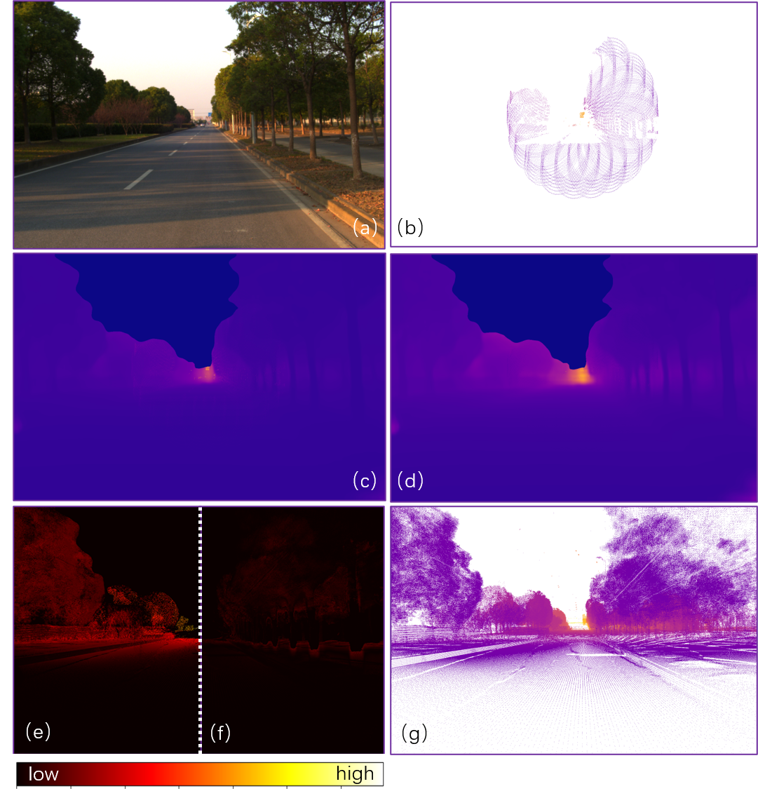
Figure 1: (a) and (b) are the input pair, i.e., reference image from RGB camera and partial depth map from MEMS LiDAR. (c) is the improved result of MonoDepth2 [8]. (d) is our depth extension result. (e) and (f) are the error map of MonoDepth2 [8] and ours respectively. (g) is the ground truth from our LEAD dataset.

Despite the irresistible trend of using MEMS LiDAR, it suffers small field of view (FoV), which slows down the step of its population. Typical mechanical LiDAR sensors are always with $360^{\circ}$ FoV, while MEMS LiDAR such as the one adopted in our paper is just $14.5^{\circ}\times 16.2^{\circ}$. A promising direction is utilizing a coupled camera with larger FoV to extend the point cloud/depth from MEMS LiDAR. A natural question to ask is: why do not we directly use cameras for depth estimation if an extra camera is introduced? It is true that depth estimation from monocular or stereo cameras, especially with the power of deep learning, achieves compelling results [2, 7, 33, 8, 5, 22]. For example, some works  [5, 7] utilize left-right consistency cues to train the monocular depth estimation network. Some online estimate poses from sequential images, and then form a photometric re-projection loss in sequence for training. Nevertheless, the depth maps estimated in this line of works suffer from scale ambiguities. They may yield plausible relative depth map, but hard to deploy in real AD systems due to the incredible scale.

Another family of works avoid the scale ambiguities with the guidance of LiDAR even only partial observations w.r.t the FoV of camera. The problem then becomes how to complete the depth maps with images [27, 23]. Regarding existing depth completion approaches, the input depth maps are projected from raw point clouds from mechanical LiDAR. Thus, the depth pattern is sparse, but covers the whole space of target view (the FoV of image). Those methods focus on inpainting holes of depth map using interpolation and propagation mechanism [13, 21]. Oppositely, as shown in fig:teaser, our MEMS LiDAR could only produce very limit observations in a small area, which usually lies on the center of coupled images. In other words, we need to extend/outpainting significantly from partial depth to fill the whole space of target image. Actually, there are few works of depth completion on line sensors [11], and they are only validated on indoor scenes. To the best of our knowledge, our approach is the first one of extending such limited depth observation to large FoV with high accuracy.

The key insight of the proposed approach is to propagate partial depth from MEMS LiDAR to a larger area with the guidance of image. We experimentally found directly propagating such small area of depth is impractical. Thus, we introduce a multi-stage propagation to deal with this problem gradually. In each stage, we extend current high confident area, which is the depth from MEMS LiDAR at the first stage, outward with a certain width. Eventually, we can get full of accurate depth after several stages. However, an effective extending operation between two stages is not trivial. Technically, in our approach, the output of one stage are a depth distribution set and an uncertainty map instead of one simple depth map. Then we use a novel probabilistic selection and combination operator to yield the depth for next state. With these mechanism, accurate depth could effectively propagate out. However, the network stays fragility even with well-designed training strategy or parameters. Thus, we propose a teacher-student training fashion to learn depth estimation ability from existing monocular depth estimation algorithm, while not mislead by its wrong scale. We build a teacher network based on Mono2[8] for our core depth outpainting/propagation network. Qualitative and quantitative experiments show that the proposed method outperforms SOTAs with a large margin. Additionally, in order to have accurate metrics, we use a 3D high-accurate long range laser scanner to collect our own dataset. In summary, the technical contributions of our work are as follows:

• We introduce a new setup focusing on extending the MEMS LiDAR by coupled image w.r.t both FoV and range. We propose a multi-stage propagation strategy based on depth distributions and uncertainty map, which shows effective propagation ability.

• We introduce a teacher-student strategy to combine monocular depth estimation and completion networks. We experimentally find such strategy could transfer depth estimation ability to depth completion network without any scale error passed.

• To validate the LiDAR extension quality, we utilize a high-precise laser scanner to generate ground-truth dataset. The dataset contains 16792 pairs of MEMS LiDAR data and image for training, as well as 120 pairs of panoramic depth with up to 5mm accuracy in 2500m range for testing. We hope such carefully collected data could benefit the community w.r.t depth researches.

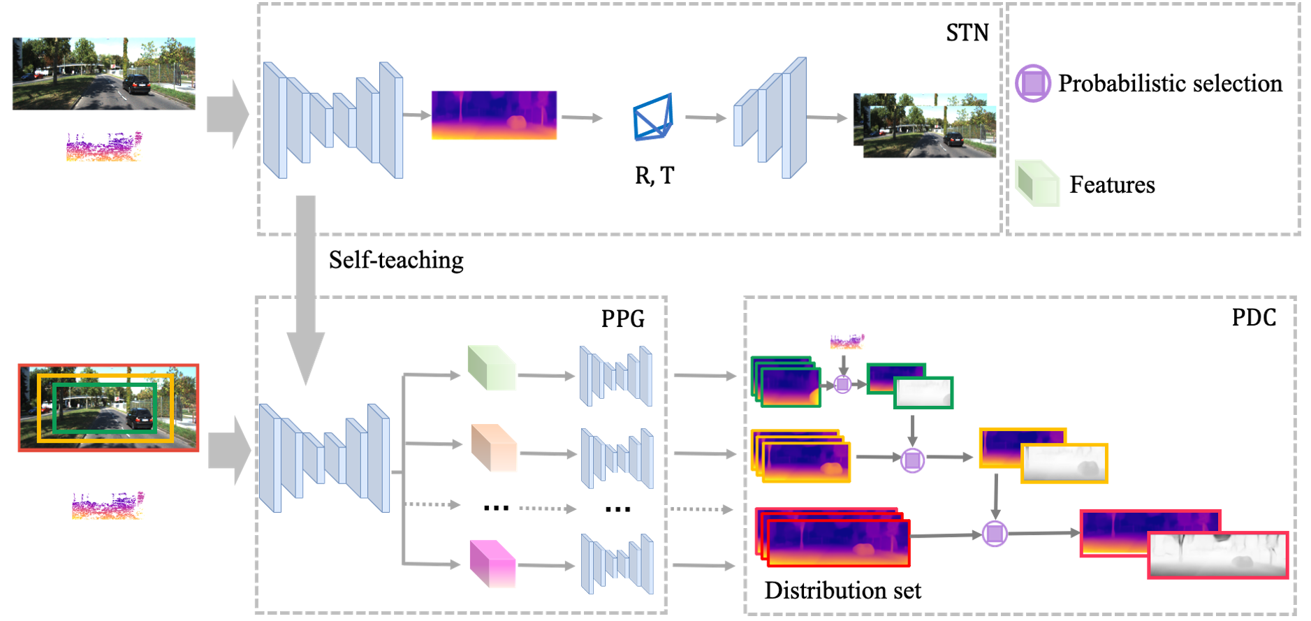
Figure 2: Overview of our method. The pipeline consists of a self-supervised teacher network (STN), propagative probabilistic generating (PPG) module and probabilistic derivation and composition (PDC) module. STN provides the initial depth and stabilizes the training processing of PPG. PPG generates the depth probabilistic distributions for different propagation levels. With these distributions and the input partial depth map, PDC derives the final depth map with corresponding uncertainty.

2 Related Work

2.1 Depth Completion

Depth completion is a high-relevant topic with our task, which focuses on yielding dense depth from sparse or noisy point cloud data [23, 20, 24]. The classical depth completion methods take only sparse or noisy depth sample from LiDAR or SLAM/SfM systems as input, which fall into the concept of depth super-resolution [16], depth inpainting [31], depth denoising [25]. In this category, Zhang et al. [32] proposed to predict the surface normal to estimate the dense depth map for indoor scenes in NYUv2 dataset[26]. Ma et al. [18] use sparse depth maps and images to first calculate the camera poses, and then train a depth completion network based on predicted poses. Those works achieve compelling results of depth densification, but they only deal with partial depth map in the same resolution with RGB image, which is sparse samples in the complete spatial space. So, the network only needs to inpaint the empty part of the depth map. However, in our setup, the input depth is only small part w.r.t the vertical and horizontal space of our final estimated depth. Our task is more a depth outpainting problem with both the FoV and range extension are required. Instead of mechanical LiDAR, Liao et al. [11] adapt a line sensor to get the partial depth measurement and generate a dense depth map but limited by the setup, this method can only be applied indoor.

In depth completion, propagating high-confidential depth samples to the whole depth map is a widely adopt mechanism. Spatial Propagation Networks (SPN) [15] trained a neural network to learn the local linear spatial propagation which can enhance the depth map or segmentation result but each time SPN updates a pixel, the whole image needs to be scanned, which affects the efficiency of the algorithm. Cheng et al. [13] proposed CSPN which focuses on the local context to propagate the depth. Since the depth value is generally closely related to the surrounding depth values, the local propagation can improve the depth map efficiently. The CSPN based method further improved efficiency by adding resource-aware module [12] and non-local information [21]. The depth propagation method also has the potential to extend the small FoV depth,  [14] propagate the small FoV depth to generate the panoramic depth.

2.2 Depth Estimation

The target of monocular depth estimation is to estimate the depth map with a single camera. This problem is ill-posed since an image can project to many plausible depths. So in practice, these methods can only provide an estimation or relative depth map. Eigen et al. [2] proposed the first learning-based monocular depth estimation algorithm relies on the dense ground truth. After this work, a lot of supervised learning based monocular depth estimation merged, such as  [4] and  [9]. However, acquisition of the accurate and dense ground truth is tedious.  [19] tried to explore the potential of synthetic training data but the complexity of synthetic data is still not comparable with the real data. To break through the limitation of insufficient training data, Gard et al. [5] proposed a self-supervised learning framework that uses the stereo pair and constructs the stereo photometric reprojection warping loss to train the network. After that, Godard et al. [7] improved stereo based framework by adding a left-right consistency loss. In addition to stereo pair, Zhou et al. [33] only used the video sequences to estimate both the camera pose and depth map and the assumption of this method is that the scene is static so the network had to predict a mask to filter out the moving objects. Godard et al. [8] also improved sequence-based self-supervised framework with an auto-mask, besides, in  [8], the two kinds of the self-supervised framework were used together, which also improved the monocular depth estimation result. To improve the quality of the depth map, some other tasks can be added and trained together, such as optical flow estimation [30] and image segmentation [34] [28]. To find the uncertain area, some algorithms [3] [10] [22] generate the uncertainty map while estimating the depth map.

However, these monocular depth estimation methods are limited by the scale ambiguity. The supervised method can only recover the scale of the dataset, the scale of the stereo based self-supervised method is up to the baseline of the training dataset and the sequence-based method needs ground truth to correct the scale, which greatly reduces the practicability of the algorithm.

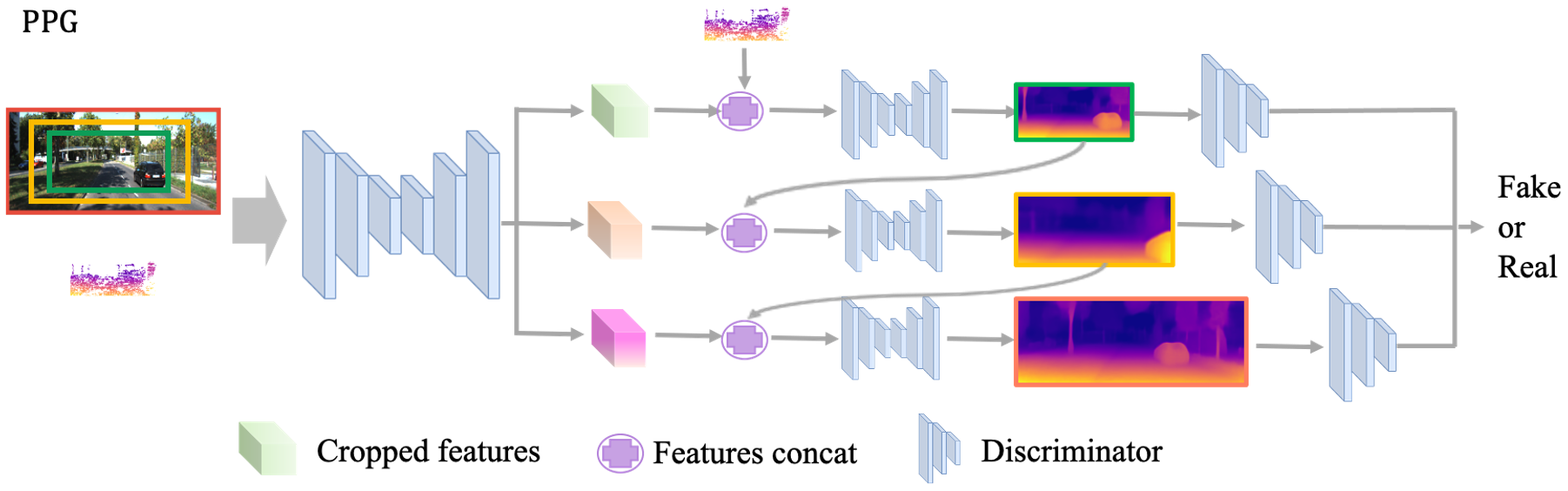
Figure 3: Propagative probabilistic generating module. For each propagation stage, the network can fuse the output depth from last stage to generate depth map for next stage. On each stage, there is a discriminator to judge the quality of generated depth map.

3 Method

3.1 Overview

Given the RGB image $I$ and partial depth map $D_{s}$ generated from MEMS LiDAR sensor, our goal is to estimate full depth map $D_{f}$ with same FoV of camera, in other words, the same resolution of image $I$. The key insight of the proposed method is to propagate the partial depth to larger areas with guidance of image. Digging into the inputs, the partial depth $D_{s}$ provide the some accurate observations, and the structure in RGB image $I$ encodes plentiful cues for depth distribution so we want to learn a mapping $G:(I,D_{s})\rightarrow p$. Due to the scale ambiguity, the mapping relationship is not unique and inspiring by [29], instead of estimating $D_{f}$ directly, our method estimate conditional depth distribution $p(D|I,D_{s})$. With the depth distribution and small FoV depth map, we can derive the depth map with right scale. In our approach, we adopt GAN to generate a set of depth maps $\{d_{1},d_{2},\cdot\cdot\cdot,d_{k}\}$ to approximate depth distribution discretely.

However, training such probabilistic generator faces some challenges. First, generating dense outdoor depth maps needs to face the challenge that acquiring the ground truth is hard. Even using the expensive lidar, there are still holes in the depth maps, so here we adopt the unsupervised training method. Second, training process is not stable, especially without ground truth. Besides, how to make full use of the partial depth and propagate the partial depth is also a problem.

To solve these challenges and extend the small FoV depth well, we propose self-supervised teacher network, probabilistic propagation generator and probabilistic derivation and composition module.

3.2 Self-supervised Teacher Network (STN)

To stabilize the training process without ground truth, we first train a teacher network to guide the probabilistic generator. The teacher network can provide the initial depth map for next stage, and the depth map can be used as the pseudo ground truth. Besides, the probabilistic generator that shares the encoder and decoder structure and initialize with the weight of teacher network can distill the knowledge learned by the teacher network. The input of our teacher net is RGB and partial depth map, however, since the effective region of partial depth map is small, if we directly concatenate the RGB and the partial depth map, the value distribution of final depth map is uneven and not smooth, to avoid this problem, we first extract features of the RGB and the partial depth map separately and concatenate the featuresa as the input of Unet.

Without ground truth, we adopt the self-supervised training method. In addition to the network for depth estimation, we construct a network for pose estimation. With the estimated pose and depth we can synthesis the target image from another viewpoint. By minimizing the photometric reprojection loss, the network can be trained to generate depth maps. The estimated pose can also be used to supervised the probabilistic generator.

3.3 Propagative Probabilistic Generator (PPG)

Based on the guidance of STN, we can build our probabilistic generator. The target of the generator is to make full use of the partial depth map and generate the depth distribution.

Multi stage propagation

In our experiments, we found that the straightforward mapping of $I,D_{s}\rightarrow p$ is unsatisfactory. This is reasonable, as $D_{s}$ could provide relatively accurate depth values but only in very limited area, which cannot effectively propagate out to the whole space. Thus depth values in remaining area heavily rely on the inference from monocular image, which cannot guarantee the accuracy. Our insight here is a multi-stage propagation mechanism to correct distribution set incrementally in spatial space. Considering the small FoV depth cannot affect the whole depth map but it can improve the nearby depth value, here we gradually expand the propagation area. For example, in the first propagation stage, we only fuse the small FoV depth with a little larger cropped depth map. During the fusion step, we pad the small FoV depth to the same size as the larger one and adjust the scale of the unrefined larger cropped depth maps based on the median ratio,

$$\begin{split}D_{i}^{s}=median(D_{i-1}>0)/median(D_{i}^{b}>0)\cdot D_{i}^{b},\\ D_{i}^{m}=(1-\text{sgn}(D_{i-1}))D_{i}^{s}+\text{sgn}(D_{i-1})D_{i-1},\end{split}$$ (1)

where $D_{i}^{b}$ is the blur depth map cropped from the output of teacher network, $D_{i-1}$ is the refined depth map in stage $i-1$, in stage $i$, $D_{i-1}$ will be padded to the same size as $D_{i}^{b}$, $D_{i}^{s}$ is the depth after scale adjustment and $D_{i}^{m}$ is the mixed depth map. Then refine depth of this stage is generated with the concatenation of cropped RGB features and depth features extracted from the $D_{i}^{m}$. In the next stage, the last stage depth maps will be propagated into a larger cropped depth map. Repeating this step can propagate the small FoV depth into the whole depth map. For each stage, the generated depth map is based on the refined depth map of the last stage.

Probabilistic Generating

After propagation, to generate the depth distribution, we introduce a distribution generating block to generate the distributions of each propagation stage.  fig:PPG shows the details of our distribution generating block. While training, at each propagation stage, the generator can generate the depth map of this stage and the discriminator will judge the quality of the generated depth map. Like other generative adversarial networks, we introduce some noise to the input feature by randomly dropping out. While testing, we still enable the function of dropping out and generate probabilistic distribution by multiple forward sampling. Additionally, we can derive the uncertainty map $U$ using standard deviation of distribution set $p(D|I,D_{s})$:

$$U=\sigma(p)=\sqrt{\frac{1}{N}\sum_{k=1}^{N}(d_{k}-\mu(p))},d_{k}\in p,$$ (2)

where $N$ is the size of distribution set $p$. $\mu(p)=\frac{1}{N}\sum_{k=1}^{N}d_{k}$ is the mean of $p$.

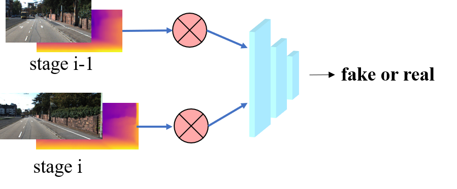
Figure 4: The training process of the discriminator. The discriminator can learn the mapping relationship between RGB and D. At stage i, we regard the RGBD set of stage i-1 as ground truth and judge whether the RGBD set of i is fake or real.

However, using the given small FoV RGBD values merely cannot train the discriminator well due to the limited field of view. We thus adopt the propagation strategy to train the GAN step by step. At each stage, the refined depth at previous stage is regarded as the true samples, while the cropped depth in this stage which aligns with RGB images of the previous stage is regarded as the false samples. In this way, the discriminator can gradually learn the right mapping function of RGB and D, and correct the depth map. Besides, for better training of the discriminator, we randomly change the scale of depth maps, i.e., in stage $i$, for the discriminator

$$\begin{split}D^{t}_{i}=S\cdot D_{i-1},D^{f}_{i}=S\cdot D_{i},\end{split}$$ (3)

where $S$ follows uniform distribution $S\sim U\text{[0.8,1.2]}$, we can change the size of the RGBD image by a random scale $S_{\text{size}}\sim U\text{[0.5,1.8]}$. The data augment forces the discriminator to learn the structural mapping relation between RGB and depth, while ignoring the different scales and sizes among different levels. In addition to the adversarial loss, we also use the pose and pseudo depth map learned by STN to train the generator.

3.4 Probabilistic Derivation and Composition

With the probabilistic depth distribution, the simple way to generate the final depth map is to calculate the mean of these distribution, however, this way cannot take advantage of partial depth map.  [29] uses optimization algorithms to post process the network results, which increases the complexity of the algorithm. However, with our special propagative probabilistic generator, we can derive the final depth map without complex post-processing. Since we generate the depth distribution at each propagation stage, we can follow the same idea to derive and compose the final depth map stage by stage. The depth map $D_{i}$ in stage $i$ can be acquired by

$$\begin{split}D_{i}=\min_{d_{k,i}\in p_{i}}(\|(d_{k,i}-D_{i-1})\cdot\text{sgn}(D_{i-1})\|\\ +\lambda\|(d_{k,i}-D_{s,i})\cdot\text{sgn}(D_{s,i})\|),\end{split}$$ (4)

where $p_{i}$ is the distribution set in $i$-th stage and in our experiment, at stage $i$, we run the generator for 5 times to generate the distribution set $p_{i}$, $D_{i-1}$ is the refined depth map in stage $i-1$, $d_{k}$ is the $k$-th depth map in $p_{i}$, $\lambda$ is the weight coefficient and $D_{s,i}$ is the cropped partial depth map whose size is the same as $D_{i}$. So in each stage, we make sure that the refined depth map is similar to the previous stage refined depth map and the partial ground truth. With $D_{i}$, the distribution of the next stage can be generated by next generator and we use the same way to generate $D_{i+1}$. In this way, we can gradually propagate the partial depth information into the final result.

3.5 Network Training

For self-supervised learning, given the camera intrinsic and the relative pose between the two frames, we can use the depth map to synthesis the image of a novel view and calculate the photo-metric loss.

$$\mathcal{L}_{pe}=F(\pi(I(t^{\prime}),K,R|t,D,I(t))),$$ (5)

$$F(I^{\prime},I)=\frac{\alpha}{2}(1-\text{SSIM}(I^{\prime},I))+\|I^{\prime}-I\|.$$ (6)

For STN, we adopt multi-scale output and use three frames to train the network. While training with three frames,

$$\mathcal{L}_{pe}=\sum_{s=0}^{4}w_{i}\min_{i\in{-1,1}}F(I(t+i),I(t)).$$ (7)

The partial depth maps can supervise the output depth maps,

$$\mathcal{L}_{part}=\sum_{s=0}^{4}\|D_{s}-\text{sgn}(D_{part})\|.$$ (8)

Besides, we use edge-aware smooth loss to improve the smoothness

$$\mathcal{L}_{smooth}=|\partial_{x}D|e^{-|\partial_{x}I|}+|\partial_{y}D|e^{-|\partial_{y}I|}.$$ (9)

The final loss function for STN is

$$\mathcal{L}_{t}=w_{pe}\mathcal{L}_{pe}+w_{p}\mathcal{L}_{part}+w_{s}\mathcal{L}_{smooth}.$$ (10)

When training the PPG, different from the STN, the output of the network are five different size depth maps corresponding to five propagation stages. The PPG follows the GAN structure, the loss function contains a GAN loss and an appearance loss. The GAN loss is

$$\mathcal{L}_{GAN}=\sum_{i=0}^{5}\mathbb{E}_{I_{i}^{t},D_{i}^{t}}[logD(I_{i}^{t},D_{i}^{t})]+\mathbb{E}_{z_{i}}[log(1-D(G(z_{i})))].$$ (11)

For appearance loss, since the STN has generated $D_{blur}$, we adjust the scale of the depth map to supervise the PPG

$$s=median(D_{part}>0)/median(D_{t}\cdot\text{sgn}(D_{part})),\\$$ (12)

$$D_{pseudo}=s\cdot D_{blur},$$ (13)

$$\mathcal{L}_{pseudo}=F(crop(D_{pseudo}),D_{s}),$$ (14)

The partial depth can adjust the scale of $D_{blur}$ to generate $D_{pseudo}$. Considering that $D_{pseudo}$ is not sufficiently accurate, we expect PPG can learn the structure of the depth map from $D_{pseudo}$ instead of the value. Thus in $L_{pseudo}$, the weight of SSIM term is larger. While training the generator, we need to adjust all the camera translations estimated by the posenet to construct the photo-metric loss,

$$\hat{t}={t}\cdot{s},$$ (15)

where $t$ is the origin pose and $\hat{t}$ is the adjusted pose. With $\hat{t}$, We construct the photo-metric loss of generator denoted as $\mathcal{L}_{peg}$, then the loss function of PPG is given by

$$\mathcal{L}_{s}=w_{peg}\mathcal{L}_{peg}+w_{pse}\mathcal{L}_{pseudo}+w_{G}\mathcal{L}_{GAN}.$$ (16)

For training, we use dropout as the random noise of the input. For testing, we still enable the dropout function work and generate the distribution sets.

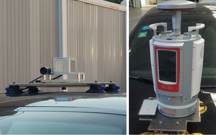
Figure 5: LEFT: MEMS LiDAR and camera hardware setup. RIGHT: the laser scanner for ground truth depth estimation.

4 Experiment

4.1 Hardware and Evaluation Dataset

Hardware

fig:setup shows the MEMS LiDAR and camera hardware setup, which is mounted on the roof of a vehicle for outdoor scanning. We use the Tele-15 MEMS LiDAR sensor from Livox Inc. as the partial depth sensor. The FoV of the MEMS LiDAR is $14.5^{\circ}\times 16.2^{\circ}$. Although the claimed depth sensing range is 500 meters, the effective range is from 3 meters to 200 meters during our practical usage. In addition, we use an industrial camera from FLIR Inc. with 12mm focal length, $41.3^{\circ}\times 31.3^{\circ}$ FoV and $1536\times 1024$ resolution. The MEMS LiDAR and camera are calibrated.

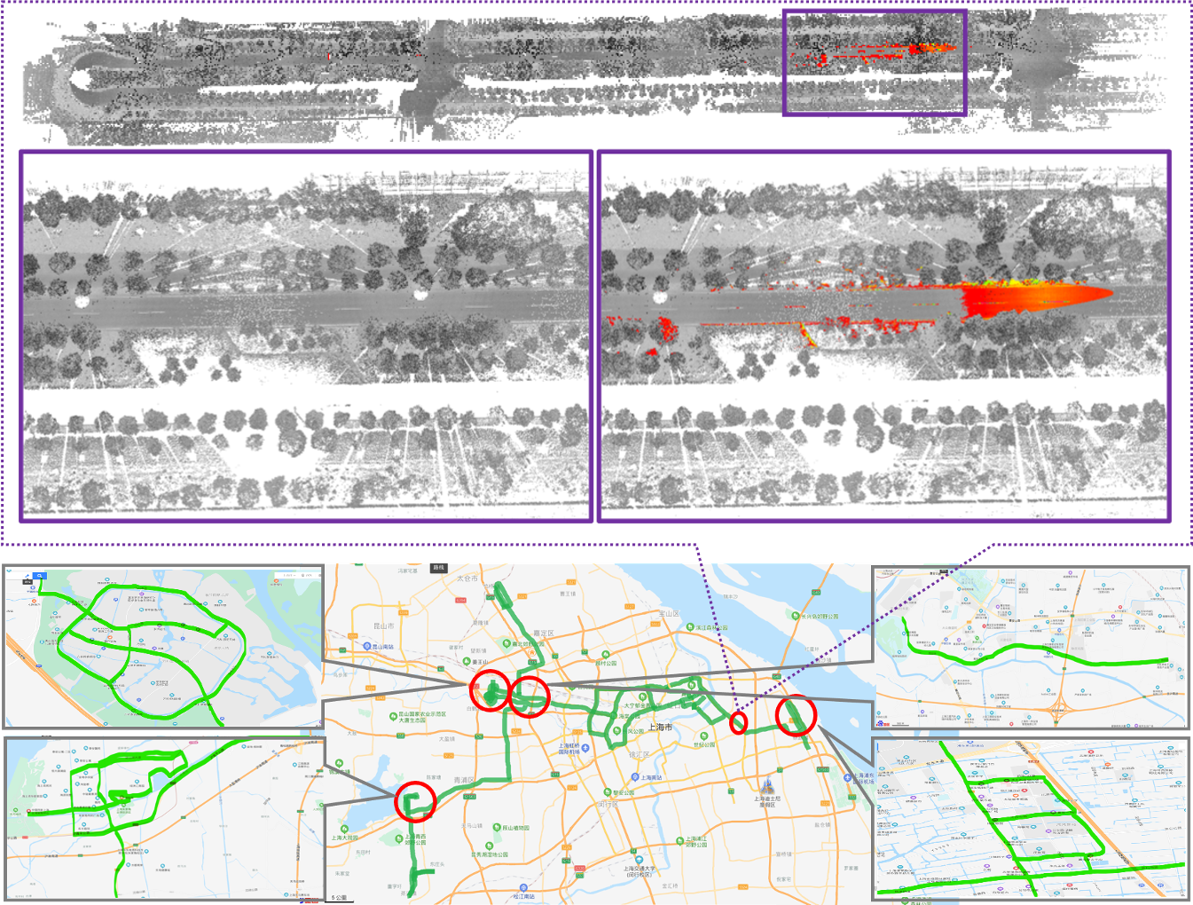
Figure 6: Collection area and samples in LEAD dataset. The map in bottom row shows the data collection area. The point clouds in dotted box are captured from MEMS LiDAR (red) and high-accurate laser scanner (grey).

Our LEAD Dataset

We captured around 100 hours data, in 50 streets over 500 kilometer from urban area in Shanghai, China. Then, we semi-automatically pick 16792 pairs of partial depth maps and their corresponding images, which are used as training and validation set. To quantitatively evaluate the extended depth map from our setup, we utilize an additional high-accurate long range laser scanner to capture additional 120 pairs with ground truth depth. We use Riegl Inc.’s vz-2000  3D terrestrial laser scanner. The scanner has a wide FoV of $100^{\circ}\times 360^{\circ}$ with up to 2500 meters sensing capability and 5 mm accuracy. We calibrate the laser scanner and the MEMS LiDAR by align the dense depth and the partial depth using point-to-plane ICP. fig:dataset shows one sample of testing set in our LEAD dataset. We are releasing the full LEAD dataset to public along with this paper. We believe it will benefit the community including but not limited to the research on MEMS LiDAR depth estimation.

KITTI Eigen Split

To evaluate the generalizability of our proposed method, we conduct experiments on the KITTI dataset [6]. However, the original KITTI dataset provides only the ground truth depth but not partial depth maps with limit FoV like those from MEMS LiDAR in our setup. We resample a small region from the ground truth to simulate partial depth input. Note that we use the improved ground truth depth maps provided by KITTI in our experiments. Since the original ground truth depth maps are rendered from point clouds captured raw mechanical LiDAR with $360^{\circ}$ FoV, which is sparse and with many holes in rendered depth maps.

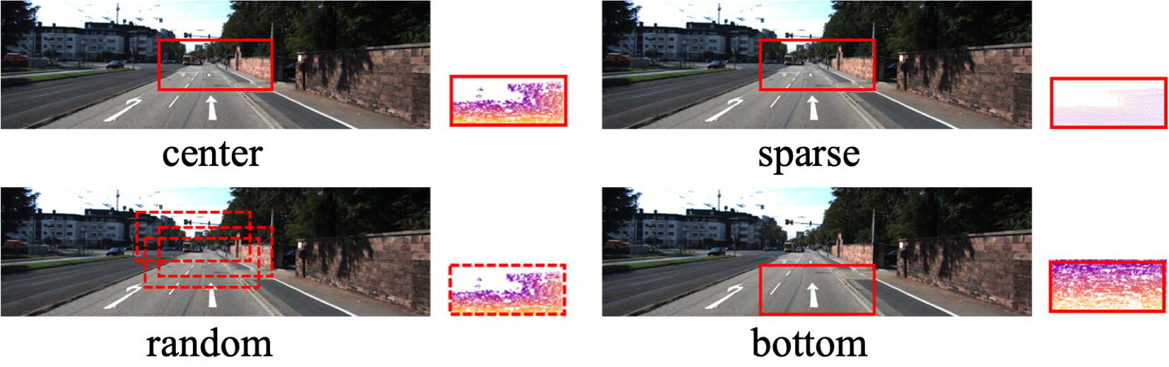
Figure 7: Different resampling modes in KITTI dataset.

Regarding resampling from the ground truth, we provide 4 modes to simulate different MEMS LiDARs with different calibration. fig:cropping_modes shows the 4 resampling modes: center cropping (center), downsampling on center cropping (sparse), random cropping at the center region (random), and bottom cropping (bottom). Center cropping is the straightforward mode to simulate small FoV LiDAR located in the center of wide FoV camera. Sparse sampling mode simulates the MEMS can only provide very sparse points in small FoV. Bottom cropping simulates MEMS LiDAR yielding points in near and narrow space w.r.t the target view. In this setup, both the FoV and depth range need to be extended. Random cropping is a challenge setup, where the valid area of MEMS LiDAR locates on our target view randomly.

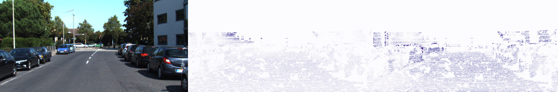
Figure 8: Qualitative results on multi-stage propagation. LEFT: the input RGB image. MIDDLE: depth map error after one stage propagation (darker color indicates more accurate depth). RIGHT: depth map error after all propagation stages.

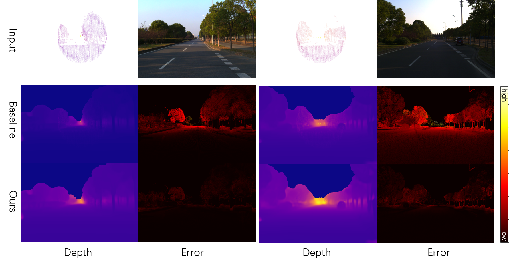
Figure 9: Qualitative results on LEAD dataset.

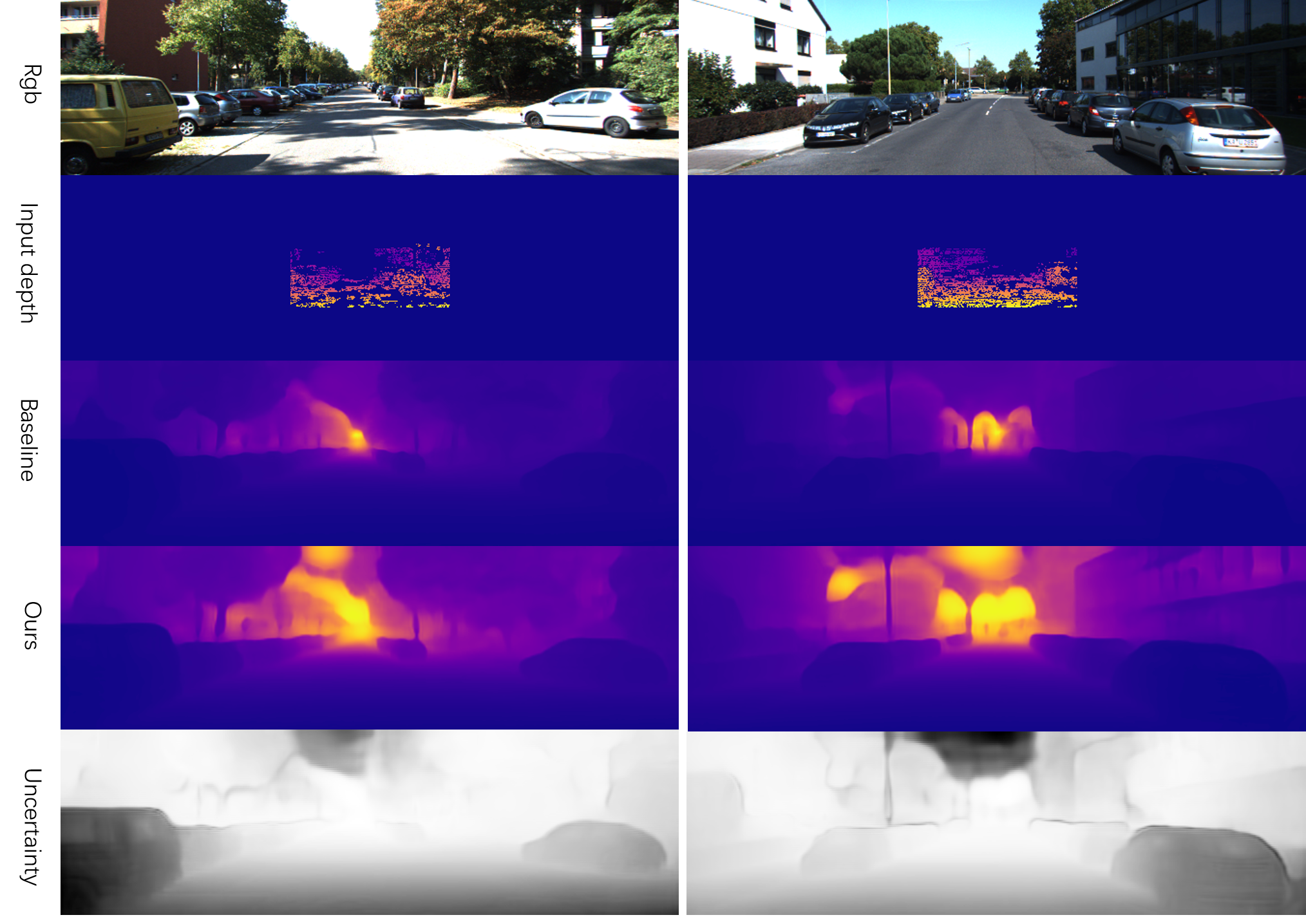
Figure 10: Qualitative results on KITTI dataset.

4.2 Qualitative Results

Multi-stage propagation

We illustrate the effectiveness of the multi-stage propagation mechanism. In particular, fig:propagation qualitative shows that the depth map error reduces after all propagation stages (RIGHT) as compared to the depth map error after a single propagation stage (MIDDLE).

Results on LEAD dataset

fig:lead qualitative shows the qualitative results on our LEAD dataset. The second row shows the depth map and its the error map for the STN module. The third row shows the results for our full pipeline.

Results on KITTI dataset

fig:kitti qualitative shows the qualitative results on the KITTI dataset. Since our network is based on MonoDepth2 [8], we use it as our baseline method. We train the MonoDepth2 supervised by the input narrow FoV depth map. MonoDepth2 suffers from the problem of sparse and uneven depth distribution. The input narrow FoV depth map is not able to correct the scale even after using the ratio of the median to correct the monocular depth scale. By contrast, our propagation and distribution output modules are designed to solve this problem, resulting more accurate wide range of depth maps.

		lower is better				higher is better
Method	SC	Abs Rel	Sq Rel	RMSE	RMSE log	$\delta_{1.25}$	$\delta_{1.25^{2}}$	$\delta_{1.25^{3}}$
EPC++[17]	M	0.120	0.789	4.755	0.177	0.856	0.961	0.987
Geonet[30]	M	0.132	0.994	5.240	0.193	0.833	0.953	0.985
MonoDepth2[8]	M	0.090	0.545	3.942	0.137	0.914	0.983	0.995
EPC++	F	0.153	0.998	5.080	0.204	0.805	0.945	0.982
Geonet	F	0.202	1.521	5.829	0.244	0.707	0.913	0.970
MonoDepth2	F	0.109	0.623	4.136	0.154	0.873	0.977	0.994
MonoDepth2	P	0.104	0.560	3.898	0.48	0.889	0.980	0.995
Ours (res18)	P	0.101	0.456	3.475	0.140	0.909	0.984	0.996
Ours (res50)	P	0.090	0.424	3.419	0.133	0.916	0.984	0.996

Table 1: Quantitative results on KITTI Eigen Split with improved ground truth. “SC” means different scale correction methods: “M” means using different scales for each individual test case. The scale is the ratio between the median depth of the ground truth depth map and the median depth of the resulting depth map. “F” means using a fixed scale that is the mean scale. “P” means using the scale estimated from the input partial depth.

	lower is better		higher is better
Method	RMSE	RMSE log	$\delta_{1.25}$	$\delta_{1.25^{2}}$	$\delta_{1.25^{3}}$
STN	15.718	0.633	0.070	0.174	0.603
Ours	6.299	0.171	0.859	0.963	0.991
STN ($<80$)	14.446	0.633	0.072	0.176	0.604
Ours ($<80$)	6.053	0.172	0.858	0.963	0.991
STN ($>80$)	22.687	0.330	0.720	0.743	0.848
Ours ($>80$)	6.968	0.077	0.959	0.999	1.000

Table 2: Quantitative results on LEAD dataset.

4.3 Quantitative Results

Results on LEAD dataset

Tab. 9 shows the quantitative results on our LEAD dataset. We compare results for the STN module and our full pipeline. Moreover, since our LEAD dataset contains ground truth depth over 80 meters that is the maximum ground truth depth provided by the KITTI dataset, we also show results using the ground truth depth less than 80 meters and larger than 80 meters respectively.

Results on KITTI dataset

Tab. 1 shows the quantitative results on the KITTI Eigen Split [1]. We compare our results with various monocular depth estimation methods. The first and second row blocks shows results for the unsupervised monocular depth estimation methods, which needs scale correction based on ground truth depth information. However, using depth information from ground truth is not a practical assumption. By contrast, our method only needs partial depth maps. Hence, the third row block shows results for MonoDepth2 and our method using partial depth map for scale correction. The results show that our method outperforms the baseline methods.

Tab. 3 shows the quantitative results of our method on KITTI dataset under different resampling modes. The results do not differ much under different resampling modes, which indicates the generalizability of our method.

Ablation Study

Tab. 4 shows the ablation study results. We compare the performances among three methods: STN, STN+PPG, and STN+PPG+PDC. STN is the normal propagation without distribution generation. STN+PPG adds the distribution generation. STN+PPG+PDC is our entire pipeline. It can be shown that the proposed PPG and PDC modules improve the performance effectively.

	lower is better		higher is better
Method	RMSE	RMSE log	$\delta_{1.25}$	$\delta_{1.25^{2}}$	$\delta_{1.25^{3}}$
Center	3.475	0.140	0.909	0.984	0.996
Sparse	3.558	0.140	0.909	0.983	0.995
Random	3.483	0.141	0.909	0.984	0.996
Bottom	3.859	0.136	0.911	0.982	0.995

Table 3: Results on different resampling modes.

	lower is better				higher is better
Method	Abs Rel	Sq Rel	RMSE	RMSE log	$\delta_{1.25}$	$\delta_{1.25^{2}}$	$\delta_{1.25^{3}}$
STN	0.103	0.504	3.713	0.148	0.886	0.979	0.995
STN+PPG	0.106	0.486	3.635	0.144	0.904	0.983	0.996
STN+PPG+PDC	0.101	0.456	3.475	0.140	0.909	0.984	0.996

Table 4: Ablation study on KITTI dataset.

5 Conclusion

We propose a novel self-supervised learning based method to use the small field of view solid-state MEMS LiDAR to estimate a deeper and wider depth map, a new hardware system, and a corresponding dataset for this kind of LiDAR. The experiment shows that our new setup and algorithm make full use of the depth generated by the MEMS LiDAR and generate a deeper and wider depth map. We believe that our setup and method can promote the wide application of the low cost and miniaturized solid-state MEMS LiDAR in the field of autonomous driving.

References

- [1] David Eigen and Rob Fergus. Predicting depth, surface normals and semantic labels with a common multi-scale convolutional architecture. In Proceedings of the IEEE international conference on computer vision, pages 2650–2658, 2015.
- [2] David Eigen, Christian Puhrsch, and Rob Fergus. Depth map prediction from a single image using a multi-scale deep network. In Advances in neural information processing systems, pages 2366–2374, 2014.
- [3] Abdelrahman Eldesokey, Michael Felsberg, Karl Holmquist, and Michael Persson. Uncertainty-aware cnns for depth completion: Uncertainty from beginning to end. In IEEE/CVF Conference on Computer Vision and Pattern Recognition (CVPR), June 2020.
- [4] Huan Fu, Mingming Gong, Chaohui Wang, Kayhan Batmanghelich, and Dacheng Tao. Deep ordinal regression network for monocular depth estimation. In Proceedings of the IEEE Conference on Computer Vision and Pattern Recognition, pages 2002–2011, 2018.
- [5] Ravi Garg, Vijay Kumar Bg, Gustavo Carneiro, and Ian Reid. Unsupervised cnn for single view depth estimation: Geometry to the rescue. In European conference on computer vision, pages 740–756. Springer, 2016.
- [6] Andreas Geiger, Philip Lenz, and Raquel Urtasun. Are we ready for autonomous driving? the kitti vision benchmark suite. In 2012 IEEE Conference on Computer Vision and Pattern Recognition, pages 3354–3361. IEEE, 2012.
- [7] Clément Godard, Oisin Mac Aodha, and Gabriel J Brostow. Unsupervised monocular depth estimation with left-right consistency. In Proceedings of the IEEE Conference on Computer Vision and Pattern Recognition, pages 270–279, 2017.
- [8] Clément Godard, Oisin Mac Aodha, Michael Firman, and Gabriel J Brostow. Digging into self-supervised monocular depth estimation. In Proceedings of the IEEE International Conference on Computer Vision, pages 3828–3838, 2019.
- [9] Xiaoyang Guo, Hongsheng Li, Shuai Yi, Jimmy Ren, and Xiaogang Wang. Learning monocular depth by distilling cross-domain stereo networks. In Proceedings of the European Conference on Computer Vision (ECCV), pages 484–500, 2018.
- [10] Adrian Johnston and Gustavo Carneiro. Self-supervised monocular trained depth estimation using self-attention and discrete disparity volume. In Proceedings of the IEEE/CVF Conference on Computer Vision and Pattern Recognition, pages 4756–4765, 2020.
- [11] Yiyi Liao, Lichao Huang, Yue Wang, Sarath Kodagoda, Yinan Yu, and Yong Liu. Parse geometry from a line: Monocular depth estimation with partial laser observation. In 2017 IEEE International Conference on Robotics and Automation (ICRA), pages 5059–5066. IEEE, 2017.
- [12] Xinjing Cheng, Peng Wang, Guan Chenye, and Ruigang Yang. Cspn++: Learning context and resource aware convolutional spatial propagation networks for depth completion. Proceedings of the AAAI Conference on Artificial Intelligence, 34:10615–10622, 04 2020.
- [13] Xinjing Cheng, Peng Wang, and Ruigang Yang. Learning depth with convolutional spatial propagation network. IEEE transactions on pattern analysis and machine intelligence, 2019.
- [14] Xinjing Cheng, Peng Wang, Yanqi Zhou, Chenye Guan, and Ruigang Yang. Ode-cnn: Omnidirectional depth extension networks. arXiv preprint arXiv:2007.01475, 2020.
- [15] Sifei Liu, Shalini De Mello, Jinwei Gu, Guangyu Zhong, Ming-Hsuan Yang, and Jan Kautz. Learning affinity via spatial propagation networks. In Advances in Neural Information Processing Systems, pages 1520–1530, 2017.
- [16] Jiajun Lu and David Forsyth. Sparse depth super resolution. In Proceedings of the IEEE Conference on Computer Vision and Pattern Recognition, pages 2245–2253, 2015.
- [17] Chenxu Luo, Zhenheng Yang, Peng Wang, Yang Wang, Wei Xu, Ram Nevatia, and Alan Yuille. Every pixel counts++: Joint learning of geometry and motion with 3d holistic understanding. arXiv preprint arXiv:1810.06125, 2018.
- [18] Fangchang Ma, Guilherme Venturelli Cavalheiro, and Sertac Karaman. Self-supervised sparse-to-dense: Self-supervised depth completion from lidar and monocular camera. In 2019 International Conference on Robotics and Automation (ICRA), pages 3288–3295. IEEE, 2019.
- [19] Nikolaus Mayer, Eddy Ilg, Philipp Fischer, Caner Hazirbas, Daniel Cremers, Alexey Dosovitskiy, and Thomas Brox. What makes good synthetic training data for learning disparity and optical flow estimation? International Journal of Computer Vision, 126(9):942–960, 2018.
- [20] Raul de Queiroz Mendes, Eduardo Godinho Ribeiro, Nicolas dos Santos Rosa, and Valdir Grassi Jr. On deep learning techniques to boost monocular depth estimation for autonomous navigation. arXiv preprint arXiv:2010.06626, 2020.
- [21] Jinsun Park, Kyungdon Joo, Zhe Hu, Chi-Kuei Liu, and In So Kweon. Non-local spatial propagation network for depth completion. arXiv preprint arXiv:2007.10042, 2020.
- [22] Matteo Poggi, Filippo Aleotti, Fabio Tosi, and Stefano Mattoccia. On the uncertainty of self-supervised monocular depth estimation. In Proceedings of the IEEE/CVF Conference on Computer Vision and Pattern Recognition, pages 3227–3237, 2020.
- [23] Jiaxiong Qiu, Zhaopeng Cui, Yinda Zhang, Xingdi Zhang, Shuaicheng Liu, Bing Zeng, and Marc Pollefeys. Deeplidar: Deep surface normal guided depth prediction for outdoor scene from sparse lidar data and single color image. In Proceedings of the IEEE Conference on Computer Vision and Pattern Recognition, pages 3313–3322, 2019.
- [24] Dmitry Senushkin, Ilia Belikov, and Anton Konushin. Decoder modulation for indoor depth completion. arXiv preprint arXiv:2005.08607, 2020.
- [25] Ju Shen and Sen-Ching S Cheung. Layer depth denoising and completion for structured-light rgb-d cameras. In Proceedings of the IEEE conference on computer vision and pattern recognition, pages 1187–1194, 2013.
- [26] Nathan Silberman, Derek Hoiem, Pushmeet Kohli, and Rob Fergus. Indoor segmentation and support inference from rgbd images. In European conference on computer vision, pages 746–760. Springer, 2012.
- [27] Jonas Uhrig, Nick Schneider, Lukas Schneider, Uwe Franke, Thomas Brox, and Andreas Geiger. Sparsity invariant cnns. In 2017 international conference on 3D Vision (3DV), pages 11–20. IEEE, 2017.
- [28] Lijun Wang, Jianming Zhang, Oliver Wang, Zhe Lin, and Huchuan Lu. Sdc-depth: Semantic divide-and-conquer network for monocular depth estimation. In Proceedings of the IEEE/CVF Conference on Computer Vision and Pattern Recognition, pages 541–550, 2020.
- [29] Zhihao Xia, Patrick Sullivan, and Ayan Chakrabarti. Generating and exploiting probabilistic monocular depth estimates. In Proceedings of the IEEE/CVF Conference on Computer Vision and Pattern Recognition, pages 65–74, 2020.
- [30] Zhichao Yin and Jianping Shi. Geonet: Unsupervised learning of dense depth, optical flow and camera pose. In Proceedings of the IEEE Conference on Computer Vision and Pattern Recognition, pages 1983–1992, 2018.
- [31] Hai-Tao Zhang, Jun Yu, and Zeng-Fu Wang. Probability contour guided depth map inpainting and superresolution using non-local total generalized variation. Multimedia Tools and Applications, 77(7):9003–9020, 2018.
- [32] Yinda Zhang and Thomas Funkhouser. Deep depth completion of a single rgb-d image. In Proceedings of the IEEE Conference on Computer Vision and Pattern Recognition, pages 175–185, 2018.
- [33] Tinghui Zhou, Matthew Brown, Noah Snavely, and David G Lowe. Unsupervised learning of depth and ego-motion from video. In Proceedings of the IEEE Conference on Computer Vision and Pattern Recognition, pages 1851–1858, 2017.
- [34] Shengjie Zhu, Garrick Brazil, and Xiaoming Liu. The edge of depth: Explicit constraints between segmentation and depth. In Proceedings of the IEEE/CVF Conference on Computer Vision and Pattern Recognition, pages 13116–13125, 2020.