Hunting for direct CP violation in $\bar{B}_{s}^{0}\to{\pi^{+}}{\pi^{-}}K^{*0}$

Abstract

In perturbative QCD approach, based on the first order of isospin symmetry breaking, we study the direct $CP$ violation in the decay of $\bar{B}_{s}^{0}\to\rho(\omega)K^{*0}\to{\pi^{+}}{\pi^{-}}K^{*0}$. An interesting mechanism is applied to enlarge the $CP$ violating asymmetry involving the charge symmetry breaking between $\rho$ and $\omega$. We find that the $CP$ violation is large by the $\rho-\omega$ mixing mechanism when the invariant masses of the $\pi^{+}\pi^{-}$ pairs is in the vicinity of the $\omega$ resonance. For the decay process of $\bar{B}^{0}_{s}\to\rho(\omega)K^{*0}\to{\pi^{+}}{\pi^{-}}K^{*0}$, the maximum $CP$ violation can reach $-59.12\%$. Furthermore, taking $\rho-\omega$ mixing into account, we calculate the branching ratio for $\bar{B}_{s}^{0}\rightarrow\rho(\omega)K^{*0}$. We also discuss the possibility of observing the predicted $CP$ violation asymmetry at the LHC.

I Introduction

Charge-Parity ($CP$) violation is an open problem, even though it has been known in the Neutral kaon systems for more than five decades Christenson:1964fg . The study of $CP$ violation in the heavy quark systems is important to our understanding of both particle physics and the evolution of the early universe. Within the standard model (SM), $CP$ violation is related to the non-zero weak complex phase angle from the Cabibbo-Kobayashi-Maskawa (CKM) matrix, which describes the mixing of the three generations of quarks Cabibbo:1963yz ; Kobayashi:1973fv . Theoretical studies predicted large $CP$ violation in the $B$ meson system Carter:1980hr ; Carter:1980tk ; Bigi:1981qs . In recent years, the LHCb collaboration has measured sizable direct CP asymmetries in the phase space of the three-body decay channels of $B^{\pm}\rightarrow\pi^{\pm}\pi^{+}\pi^{-}$ and $B^{\pm}\rightarrow K^{\pm}\pi^{+}\pi^{-}$ Aaij:2013bla ; Aaij:2014iva ; Bediaga:2020qxg . These processes are also valuable for studying the mechanism of multi-body heavy meson decays. Hence, more attention has been focused on the non-leptonic $B$ meson three-body decays channels in searching for $CP$ violation, both theoretically and experimentally.

Direct $CP$ violation in $b$ hadron decays occurs through the interference of at least two amplitudes with different weak phase $\phi$ and strong phase $\delta$. The weak phase difference $\phi$ is determined by the CKM matrix elements, while the strong phase can be produced by the hadronic matrix elements and interference between the intermediate states. The hadronic matrix elements are not still well determined by the theoretical approach. The mechanism of two-body $B$ decay is still not quite clear, although many physicists are devoted to this field. Many factorization approaches have been developed to calculate the two-body hadronic decays, such as the naive factorization approach Fakirov:1977ta ; Cabibbo:1977zv ; Wirbel:1985ji ; Bauer:1986bm , the QCD factorization (QCDF) Beneke:1999br ; Beneke:2000ry ; Sachrajda:2001uv ; Beneke:2001ev ; Beneke:2003zv , perturbative QCD (pQCD) Lu:2000em ; Keum:2000ph ; Keum:2000wi , and soft-collinear effective theory (SCET) Bauer:2000yr ; Bauer:2001cu ; Bauer:2001yt . Most factorization approaches are based on heavy quark expansion and light-cone expansion in which only the leading power or part of the next to leading power contributions are calculated to compare with the experiments. However, the different methods may present different strong phases so as to affect the value of the $CP$ violation. Meanwhile, in order to have a large signal of $CP$ violation, we need appeal to some phenomenological mechanism to obtain a large strong phase $\delta$. In Refs. Enomoto:1996cv ; Guo:1998eg ; Guo:2000uc ; Leitner:2002xh ; Lu:2010vb ; Lu:2011zzf , the authors studied direct $CP$ violation in hadronic $B$ (include $B_{s}$ and $\Lambda_{b}$) decays through the interference of tree and penguin diagrams, where $\rho$-$\omega$ mixing was used for this purpose in the past few years and focused on the naive factorization and QCD factorization approaches. This mechanism was also applied to generalize the pQCD approach to the three-body non-leptonic decays in ${B^{0,\pm}}\to{\pi^{0,\pm}}{\pi^{+}}{\pi^{-}}$ and $B_{c}\rightarrow D_{(s)}^{+}\pi^{+}\pi^{-}$ where even larger $CP$ violation may be possible Lu:2013jma ; Lu:2016lgc . In this paper, we will investigate direct $CP$ violation of the decay process $\bar{B}^{0}_{s}\to\rho(\omega)K^{*0}\to{\pi^{+}}{\pi^{-}}K^{*0}$ involving the same mechanism in the pQCD approach.

Three-body decays of heavy $B$ mesons are more complicated than the two-body decays as they receive both resonant and non-resonant contributions. Unlike the two-body case, to date we still do not have effective theories for hadronic three-body decays, though attempts along the framework of pQCD and QCDF have been used in the past Krankl:2015fha ; Wang:2014ira ; Chen:2002th ; Qi:2018syl . As a working starting point, we intend to study $\rho$-$\omega$ mixing effect in three-body decays of the $B$ meson. The $\rho$-$\omega$ mixing mechanism is caused by the isospin symmetry breaking from the mixing between the $u$ and $d$ flavors Fritzsch:2000pg ; Fritzsch:2001aj . In Ref. OConnell:1995nse , the authors studied the $\rho-\omega$ mixing and the pion form factor in the time-like region, where $\rho-\omega$ mixing comes from three part contributions: two from the direct coupling of the quasi-two-body decay of $\bar{B}^{0}_{s}\to\rho K^{*0}\to\pi^{+}\pi^{-}K^{*0}$ and $\bar{B}^{0}_{s}\to\omega K^{*0}\to\pi^{+}\pi^{-}K^{*0}$ and the other from the interference of $\bar{B}^{0}_{s}\to\omega K^{*0}\to\rho K^{*0}\to\pi^{+}\pi^{-}K^{*0}$ mixing. Generally speaking, the amplitudes of their contributions: $\bar{B}^{0}_{s}\to\rho K^{*0}\to\pi^{+}\pi^{-}K^{*0}$ $>$ $\bar{B}^{0}_{s}\to\omega K^{*0}\to\rho K^{*0}\to\pi^{+}\pi^{-}K^{*0}$ $>$ $\bar{B}^{0}_{s}\to\omega K^{*0}\to\pi^{+}\pi^{-}K^{*0}$. $\omega\to\pi^{+}\pi^{-}$ and $\omega\to\rho\to\pi^{+}\pi^{-}$ were used to obtain the (effective) mixing matrix element $\widetilde{\Pi}_{\rho\omega}(s)$ Bernicha:1994re ; Maltman:1996kj ; OConnell:1997ggd . The magnitude has been determined by the pion form factor through the data from the cross section of ${e^{+}}{e^{-}}\to{\pi^{+}}{\pi^{-}}$ in the $\rho$ and $\omega$ resonance region OConnell:1995nse ; OConnell:1996amv ; OConnell:1997ggd ; Wolfe:2009ts ; Wolfe:2010gf . Recently, isospin symmetry breaking was discussed by incorporating the vector meson dominance (VMD) model in the weak decay process of the meson Gardner:1997yx ; Guo:1999ip ; Guo:2000uc ; Lu:2016lgc ; Lu:2014uja ; Li:2019xwh . However, one can find that $\rho-\omega$ mixing produces the large $CP$ violation from the effect of isospin symmetry breaking in the three and four bodies decay process. Hence, in this paper, we shall follow the method of Refs. Gardner:1997yx ; Guo:1999ip ; Guo:2000uc ; Lu:2016lgc ; Lu:2014uja ; Li:2019xwh to investigate the decay process of $\bar{B}^{0}_{s}\to\rho(\omega)K^{*0}\to{\pi^{+}}{\pi^{-}}K^{*0}$ by isospin symmetry breaking.

The remainder of this paper is organized as follows. In Sec. II we will present the form of the effective Hamiltonian and briefly introduce the pQCD framework and wave functions. In Sec. III we give the calculating formalism and details of the $CP$ violation from $\rho-\omega$ mixing in the decay process $\bar{B}_{s}^{0}\to\rho(\omega)K^{*0}\to{\pi^{+}}{\pi^{-}}K^{*0}$. In Sec. IV we calculate the branching ratio for decay process of $\bar{B}^{0}_{s}\rightarrow\rho^{0}(\omega)K^{*0}$. In Sec. V we show the input parameters. We present the numerical results in Sec. VI. Summary and discussion are included in Sec. VII. The related function defined in the text are given in Appendix.

II The FrameWork

Based on the operator product expansion, the effective weak Hamiltonian for the decay processes $\bar{B}_{s}^{0}\to\rho^{0}(\omega)K^{*0}$ can be expressed as Buchalla:1995vs

$${\cal H}_{eff} = \frac{G_{F}}{\sqrt{2}}\Bigg{\{}V_{ub}V_{ud}^{\ast}\Big{[}C_{1}({\mu})Q^{u}_{1}({\mu})+C_{2}({\mu})Q^{u}_{2}({\mu})\Big{]}-V_{tb}V_{td}^{\ast}\Big{[}{\sum\limits_{i=3}^{10}}C_{i}({\mu})Q_{i}({\mu})\Big{]}\Bigg{\}}+\mbox{H.c.},\vspace{2mm}$$ (1)

where $G_{F}$ represents the Fermi constant, $C_{i}(\mu)$ (i=1,…,10) are the Wilson coefficients, and $V_{ub}$, $V_{ud}$, $V_{tb}$, and $V_{td}$ are the CKM matrix element. The operators $O_{i}$ have the following forms:

$$O^{u}_{1} = \bar{d}_{\alpha}\gamma_{\mu}(1-\gamma_{5})u_{\beta}\bar{u}_{\beta}\gamma^{\mu}(1-\gamma_{5})b_{\alpha},$$

$$O^{u}_{2} = \bar{d}\gamma_{\mu}(1-\gamma_{5})u\bar{u}\gamma^{\mu}(1-\gamma_{5})b,$$

$$O_{3} = \bar{d}\gamma_{\mu}(1-\gamma_{5})b\sum_{q^{\prime}}\bar{q}^{\prime}\gamma^{\mu}(1-\gamma_{5})q^{\prime},$$

$$O_{4} = \bar{d}_{\alpha}\gamma_{\mu}(1-\gamma_{5})b_{\beta}\sum_{q^{\prime}}\bar{q}^{\prime}_{\beta}\gamma^{\mu}(1-\gamma_{5})q^{\prime}_{\alpha},$$

$$O_{5} = \bar{d}\gamma_{\mu}(1-\gamma_{5})b\sum_{q^{\prime}}\bar{q}^{\prime}\gamma^{\mu}(1+\gamma_{5})q^{\prime},$$

$$O_{6} = \bar{d}_{\alpha}\gamma_{\mu}(1-\gamma_{5})b_{\beta}\sum_{q^{\prime}}\bar{q}^{\prime}_{\beta}\gamma^{\mu}(1+\gamma_{5})q^{\prime}_{\alpha},$$

$$O_{7} = \frac{3}{2}\bar{d}\gamma_{\mu}(1-\gamma_{5})b\sum_{q^{\prime}}e_{q^{\prime}}\bar{q}^{\prime}\gamma^{\mu}(1+\gamma_{5})q^{\prime},$$

$$O_{8} = \frac{3}{2}\bar{d}_{\alpha}\gamma_{\mu}(1-\gamma_{5})b_{\beta}\sum_{q^{\prime}}e_{q^{\prime}}\bar{q}^{\prime}_{\beta}\gamma^{\mu}(1+\gamma_{5})q^{\prime}_{\alpha},$$

$$O_{9} = \frac{3}{2}\bar{d}\gamma_{\mu}(1-\gamma_{5})b\sum_{q^{\prime}}e_{q^{\prime}}\bar{q}^{\prime}\gamma^{\mu}(1-\gamma_{5})q^{\prime},$$

$$O_{10} = \frac{3}{2}\bar{d}_{\alpha}\gamma_{\mu}(1-\gamma_{5})b_{\beta}\sum_{q^{\prime}}e_{q^{\prime}}\bar{q}^{\prime}_{\beta}\gamma^{\mu}(1-\gamma_{5})q^{\prime}_{\alpha},\vspace{2mm}$$ (2)

where $\alpha$ and $\beta$ are SU(3) color indices, $e_{q^{\prime}}$ is the electric charge of quark $q^{\prime}$ in the unit of $|e|$, and the sum extend over $q^{\prime}=u,d,s,c$ or $b$ quarks. In Eq. (2) $O_{1}^{u}$ and $O_{2}^{u}$ are tree operators, $O_{3}$–$O_{6}$ are QCD penguin operators and $O_{7}$–$O_{10}$ are the operators associated with electroweak penguin diagrams.

The Wilson coefficient $C_{i}(\mu)$ in Eq. (1) describes the coupling strength for a given operator and summarizes the physical contributions from scales higher than $\mu$ Buras:1998raa . They are calculable perturbatively with the renormalization group improved perturbation theory. Usually, the scale $\mu$ is chosen to be of order ${\cal O}(m_{b})$ for $B$ meson decays. Since we work in the leading order of perturbative QCD ($O(\alpha_{s})$), it is consistent to use the leading order Wilson coefficients. So, we use numerical values of $C_{i}(m_{b})$ as follow Keum:2000wi ; Lu:2000em :

$$C_{1} = -0.2703,\;\;\;\;\;\;\,C_{2}=1.1188,$$

$$C_{3} = 0.0126,\;\;\;\;\;\;\;\;\;\;C_{4}=-0.0270,$$

$$C_{5} = 0.0085,\;\;\;\;\;\;\;\;\;\;C_{6}=-0.0326,$$

$$C_{7} = 0.0011,\;\;\;\;\;\;\;\;\;\;C_{8}=0.0004,$$

$$C_{9} = -0.0090,\;\;\;\;\;\;\;C_{10}=0.0022.\vspace{2mm}$$ (3)

The combinations $a_{1}$–$a_{10}$ of the Wilson coefficients are defined as usual Ali:1998eb ; Ali:1998gb ; Keum:2000ms ; Lu:2000hj :

$$a_{1} = C_{2}+C_{1}/3,\;\;\;\;\;\;a_{2}=C_{1}+C_{2}/3,$$

$$a_{i} = C_{i}+C_{i\pm 1}/3,\;\;\;(i=3-10),\vspace{2mm}$$ (4)

where the upper (lower) sign applies, when $i$ is odd (even).

For the two-body decay processes of $\bar{B}_{s}^{0}\to M_{2}M_{3}$, we denote the emitted or annihilated meson as $M_{2}$ while the recoiling meson is $M_{3}$. The meson $M_{2}$ ($\rho$ or $\omega$) and the final-state meson $M_{3}$ ($K^{*0}$) move along the direction of $n=(1,0,{\bf{0}}_{T})$ and $v=(0,1,{\bf{0}}_{T})$ in the light-cone coordinates, respectively. The decay amplitude can be expressed as the convolution of the wave functions $\phi_{B_{s}}$, $\phi_{M_{2}}$ and $\phi_{M_{3}}$ and the hard scattering kernel $T_{H}$ in the pQCD. The pQCD factorization theorem has been developed for the two-body non-leptonic heavy meson decays, based on the formalism of Botts, Lepage, Brodsky and Sterman Chang:1996dw ; Yeh:1997rq ; Lepage:1980fj ; Botts:1989kf . The basic idea of the pQCD approach is that it takes into account the transverse momentum of the valence quarks in the hadrons which results in the Sudakov factor in the decay amplitude. Then, the decay channels of $\bar{B}_{s}^{0}\to\rho^{0}(\omega)K^{*0}$ are conceptually written as the following:

$$A(\bar{B}_{s}^{0}\to\rho^{0}(\omega)K^{*0})=\int\!\!d^{4}k_{1}d^{4}k_{2}d^{4}k_{3}\ \mathrm{Tr}\bigl{[}C(t)\phi_{B_{s}}(k_{1})\phi_{M2}(k_{2})\phi_{M3}(k_{3})T_{H}(k_{1},k_{2},k_{3},t)\bigr{]},$$ (5)

where $k_{i}(i=1,2,3)$ are momentum of light quark in each meson. $\mathrm{Tr}$ denotes the trace over Dirac structure and color indices. $C(t)$ is the short distance Wilson coefficients at the hard scale $t$. The meson wave functions $\phi_{B_{s}}$ and $\phi_{M}(m=2,3)$, including all non-perturbative contribution during the hadronization of mesons, can be extracted from experimental data or other non-perturbative methods. The hard kernel $T_{H}(k_{1},k_{2},k_{3},t)$ describes the four quark operator and the spectator quark connected by a hard gluon, which can be perturbatively calculated including all possible Feynman diagrams of the factorizable and non-factorizable contributions without end-point singularity.

The $\rho^{0}(\omega)$ and $K^{*0}$ mesons are treated as a light-light system. At the $B_{s}$ meson rest frame, they are moving very fast. We define the ratios ${r_{K^{*0}}}=\frac{M_{K^{*}0}}{M_{B_{s}}}$, ${r_{\rho}}=\frac{M_{\rho}}{M_{B_{s}}}$ and ${r_{\omega}}=\frac{M_{\omega}}{M_{B_{s}}}$. In the limit ${M_{K^{*0}}}$, ${M_{\rho}}$, ${M_{\omega}}$ $\to 0$, one can drop the terms of proportional to $r_{K^{*0}}^{2}$, $r_{\rho}^{2}$, $r_{\omega}^{2}$ safely. The symbols $P_{B}$, $P_{2}$ and $P_{3}$ refer to the $\bar{B}_{s}^{0}$ meson momentum, the $\rho^{0}(\omega)$ meson momentum, and the final-state $K^{*0}$ meson momentum, respectively. The momenta of the participating mesons in the rest frame of the $B_{s}$ meson can be written as:

$$P_{B} = \frac{M_{B_{s}}}{\sqrt{2}}(1,1,{\bf{0}}_{T}),\;\;P_{2}=\frac{M_{B_{s}}}{\sqrt{2}}(1,0,{\bf{0}}_{T}),\;\;P_{3}=\frac{M_{B_{s}}}{\sqrt{2}}(0,1,{\bf{0}}_{T}).$$ (6)

One can denote the light (anti-)quark momenta $k_{1}$, $k_{2}$ and $k_{3}$ for the initial meson $\bar{B}_{s}^{0}$, and the final mesons $\rho^{0}(\omega)$ and $K^{*0}$, respectively. We can choose:

$$k_{1} = (x_{1}\frac{M_{B_{s}}}{\sqrt{2}},0,{\bf k}_{1\perp}),\;\;k_{2}=(x_{2}\frac{M_{B_{s}}}{\sqrt{2}},0,{\bf k}_{2\perp}),\;\;k_{3}=(0,x_{3}\frac{M_{B_{s}}}{\sqrt{2}},{\bf k}_{3\perp}),$$ (7)

where $x_{1}$, $x_{2}$ and $x_{3}$ are the momentum fraction. ${\bf k}_{1\perp}$, ${\bf k}_{2\perp}$ and ${\bf k}_{3\perp}$ refer to the transverse momentum of the quark, respectively. To extract the helicity amplitudes, we parameterize the following longitudinal polarization vectors of the $\rho^{0}(\omega)$ and $K^{*0}$ as following:

$$\epsilon_{2}(L)=\frac{P_{2}}{M_{\rho(\omega)}}-\frac{M_{\rho(\omega)}}{P_{2}\cdot v}v,\;\;\;\;\epsilon_{3}(L)=\frac{P_{3}}{M_{K^{*0}}}-\frac{M_{K^{*0}}}{P_{3}\cdot n}n,$$ (8)

which satisfy the orthogonality relationship of $\epsilon_{2}(L)\cdot P_{2}=\epsilon_{3}(L)\cdot P_{3}=0$, and the normalization of $\epsilon_{2}^{2}(L)=\epsilon_{3}^{2}(L)=-1$. The transverse polarization vectors can be adopted directly as

$$\epsilon_{2}(T)=\left(0,0,{\bf{1}}_{T}\right),\quad\epsilon_{3}(T)=\left(0,0,{\bf{1}}_{T}\right).$$ (9)

Within the pQCD framework, both the initial and the final state meson wave functions and distribution amplitudes are important as non-perturbative input parameters. For the $B_{s}$ meson, the wave function of the meson can be expressed as

$$\Phi_{B_{s}}=\frac{i}{\sqrt{6}}(\not\!P_{B_{s}}+M_{B_{s}})\gamma_{5}\phi_{B_{s}}(k),$$ (10)

where the distribution amplitude $\phi_{B_{s}}$ is shown in Refs. Ali:2007ff ; Li:2004ep ; Wang:2014mua :

$$\phi_{B_{s}}(x,b)=N_{B_{s}}x^{2}(1-x)^{2}\exp\left[-\frac{M_{B_{s}}^{2}\ x^{2}}{2\omega_{b}^{2}}-\frac{1}{2}(\omega_{b}b)^{2}\right].$$ (11)

The shape parameter $\omega_{b}$ is a free parameter and $N_{B_{s}}$ is a normalization factor. Based on the studies of the light-cone sum rule, lattice QCD or be fitted to the measurements with good precision Li:2003yj , we take $\omega_{b}=0.50~{}\mathrm{GeV}$ for the $B_{s}$ meson. The normalization factor $N_{B_{s}}$ depends on the values of the shape parameter $\omega_{b}$ and decay constant $f_{B_{s}}$, which is defined through the normalization relation $\int_{0}^{1}{dx{\phi_{{B_{s}}}}\left({x,0}\right)}={f_{{B_{s}}}}/(2\sqrt{6})$.

The distribution amplitudes of vector meson(V=$\rho$, $\omega$ or $K^{*}$), $\phi_{V}$, $\phi_{V}^{T}$, $\phi^{t}_{V}$, $\phi^{s}_{V}$, $\phi^{v}_{V}$, and $\phi^{a}_{V}$, can be written in the following form Ball:1998ff ; Ball:2004rg :

$$\phi_{\rho}(x) = \frac{3f_{\rho}}{\sqrt{6}}x(1-x)\left[1+0.15C_{2}^{3/2}(t)\right]\;,$$ (12)

$$\phi_{\omega}(x) = \frac{3f_{\omega}}{\sqrt{6}}x(1-x)\left[1+0.15C_{2}^{3/2}(t)\right]\;,$$ (13)

$$\phi_{K^{*}}(x) = \frac{3f_{K^{*}}}{\sqrt{6}}x(1-x)\left[1+0.03C_{1}^{3/2}(t)+0.11C_{2}^{3/2}(t)\right]\;,$$ (14)

$$\phi_{\rho}^{T}(x) = \frac{3f_{\rho}^{T}}{\sqrt{6}}x(1-x)\left[1+0.14C_{1}^{3/2}(t)\right]\;,$$ (15)

$$\phi_{\omega}^{T}(x) = \frac{3f_{\omega}^{T}}{\sqrt{6}}x(1-x)\left[1+0.14C_{1}^{3/2}(t)\right]\;,$$ (16)

$$\phi_{K^{*}}^{T}(x) = \frac{3f_{K^{*}}^{T}}{\sqrt{6}}x(1-x)\left[1+0.04C_{1}^{3/2}(t)+0.10C_{2}^{3/2}(t)\right]\;,$$ (17)

$$\phi^{t}_{V}(x) = \frac{3f^{T}_{V}}{2\sqrt{6}}t^{2}\;,$$ (18)

$$\phi^{s}_{V}(x) = \frac{3f_{V}^{T}}{2\sqrt{6}}(-t)\;,$$ (19)

$$\phi_{V}^{v}(x) = \frac{3f_{V}}{8\sqrt{6}}(1+t^{2})\;,$$ (20)

$$\phi_{V}^{a}(x) = \frac{3f_{V}}{4\sqrt{6}}(-t)\;,$$ (21)

where $t=2x-1$. Here $f_{V}^{(T)}$ is the decay constant of the vector meson with longitudinal(transverse) polarization. The Gegenbauer polynomials $C^{\nu}_{n}(t)$ can be defined as Fan:2012kn ; Huang:2005if :

$$C^{3/2}_{1}(t) = 3t$$ (22)

$$C_{2}^{3/2}(t) = \frac{3}{2}(5t^{2}-1).$$ (23)

III $CP$ violation in $\bar{B}_{s}^{0}\to\rho^{0}(\omega)K^{*0}\to{\pi^{+}}{\pi^{-}}K^{*0}$ decay process

III.1 Formalism

The decay width $\Gamma$ for the processes of $\bar{B}_{s}^{0}\to\rho^{0}(\omega)K^{*0}$ is given by

$$\Gamma=\frac{{{P_{c}}}}{{8\pi M_{{B_{s}}}^{2}}}\sum\limits_{\sigma=L,T}{{A^{(\sigma)\dagger}}{A^{(\sigma)}}},$$ (24)

where $P_{c}$ is the absolute value of the three-momentum of the final state mesons. The decay amplitude $A^{(\sigma)}$ which is decided by QCD dynamics will be calculated later in pQCD factorization approach. The superscript $\sigma$ denotes the helicity states of the two vector mesons with the longitudinal (transverse) components L(T). The amplitude $A^{(\sigma)}$ for the decays $B_{s}(P_{B_{s}})\to V_{\rho(\omega)}(P_{2},\epsilon^{*}_{2\mu})+V_{K^{*0}}(P_{3},\epsilon^{*}_{3\mu})$ can be decomposed as follows Zhu:2005rx ; Huang:2005if ; Lu:2005be ; Li:2004ti :

$$A^{(\sigma)}=M^{2}_{B_{s}}A_{L}+M^{2}_{B_{s}}A_{N}\epsilon^{*}_{2}(\sigma=T)\cdot\epsilon^{*}_{3}(\sigma=T)+iA_{T}\epsilon^{\alpha\beta\gamma\rho}\epsilon^{*}_{2\alpha}(\sigma)\epsilon^{*}_{3\beta}(\sigma)P_{2\gamma}P_{3\rho}\;,$$ (25)

where $\epsilon^{*}$ is the polarization vector of the vector meson. The amplitude $A_{i}$ ($i$ refer to the three kinds of polarizations, longitudinal (L), normal (N) and transverse (T)) can be written as

$$M^{2}_{B_{s}}A_{L} = a\,\,\epsilon_{2}^{*}(L)\cdot\epsilon_{3}^{*}(L)+{\frac{b}{M_{2}M_{3}}}\epsilon_{2}^{*}(L)\cdot P_{3}\,\,\epsilon_{3}^{*}(L)\cdot P_{2}\;,$$

$$M^{2}_{B_{s}}A_{N} = a\;,$$

$$A_{T} = {\frac{c}{M_{2}M_{3}}}\;,$$ (26)

where $a$, $b$ and $c$ are the Lorentz-invariant amplitudes. $M_{2}$ and $M_{3}$ are the masses of the vector mesons $\rho^{0}(\omega)$ and $K^{*0}$, respectively.

The longitudinal $H_{0}$ and transverse $H_{\pm}$ of helicity amplitudes can be expressed

$$H_{0} = M^{2}_{B_{s}}A_{L},$$

$$H_{\pm} = M^{2}_{B_{s}}A_{N}\mp M_{2}M_{3}\sqrt{\kappa^{2}-1}A_{T},$$ (27)

where $H_{0}$ and $H_{\pm}$ are the penguin-level and tree-level helicity amplitudes of the decay process $\bar{B}_{s}^{0}\to\rho(\omega)K^{*0}\to{\pi^{+}}{\pi^{-}}K^{*0}$ from the three kinds of polarizations, respectively. The helicity summation satisfy the relation

$$\sum\limits_{\sigma=L,R}{{A^{(\sigma)\dagger}}{A^{(\sigma)}}}=|H_{0}|^{2}+|H_{+}|^{2}+|H_{-}|^{2}.$$ (28)

In the vector meson dominance model Nambu:1997vw ; Sakurai:1969zz , the photon propagator is dressed by coupling to vector mesons. Based on the same mechanism, $\rho-\omega$ mixing was proposed and later gradually applied to $B$ meson physics Gardner:1997qk ; OConnell:1995nse ; Lu:2010vb ; Gardner:1997yx . According to the effective Hamiltonian, the amplitude $A$ ($\bar{A}$) for the three-body decay process $\bar{B}_{s}^{0}\to{\pi^{+}}{\pi^{-}}K^{*0}$ ($B_{s}^{0}\to{\pi^{+}}{\pi^{-}}\bar{K}^{*0}$) can be written as Gardner:1997yx :

$$A = \big{<}\pi^{+}\pi^{-}K^{*0}|H^{T}|\bar{B}_{s}^{0}\big{>}+\big{<}\pi^{+}\pi^{-}K^{*0}|H^{P}|\bar{B}_{s}^{0}\big{>},$$ (29)

$$\bar{A} = \big{<}\pi^{+}\pi^{-}\bar{K}^{*0}|H^{T}|{B}_{s}^{0}\big{>}+\big{<}\pi^{+}\pi^{-}\bar{K}^{*0}|H^{P}|{B}_{s}^{0}\big{>},$$ (30)

where $H^{T}$ and $H^{P}$ are the Hamiltonian for the tree and penguin operators, respectively.

The relative magnitude and phases between the tree and penguin operator contribution are defined as follows:

$$A = \big{<}\pi^{+}\pi^{-}K^{*0}|H^{T}|\bar{B}_{s}^{0}\big{>}[1+re^{i(\delta+\phi)}],$$ (31)

$$\bar{A} = \big{<}\pi^{+}\pi^{-}\bar{K}^{*0}|H^{T}|{B}_{s}^{0}\big{>}[1+re^{i(\delta-\phi)}],$$ (32)

where $\delta$ and $\phi$ are strong and weak phases differences, respectively. The weak phase difference $\phi$ can be expressed as a combination of the CKM matrix elements, and it is $\phi=\arg[(V_{tb}V_{td}^{*})/(V_{ub}V_{ud}^{*})]$ for the $b\to d$ transition. The parameter $r$ is the absolute value of the ratio of tree and penguin amplitudes:

$$r\equiv\Bigg{|}\frac{\big{<}\pi^{+}\pi^{-}K^{*0}|H^{P}|\bar{B}_{s}^{0}\big{>}}{\big{<}\pi^{+}\pi^{-}K^{*0}|H^{T}|\bar{B}_{s}^{0}\big{>}}\Bigg{|}.$$ (33)

The parameter of $CP$ violating asymmetry, $A_{CP}$, can be written as

$$A_{CP}=\frac{|A|^{2}-|\bar{A}|^{2}}{|A|^{2}+|\bar{A}|^{2}}=\frac{-2(T_{0}^{2}r_{0}\sin\delta_{0}+T_{+}^{2}r_{+}\sin\delta_{+}+T_{-}^{2}r_{-}\sin\delta_{-})\sin\phi}{\sum_{i=0+-}T_{i}^{2}(1+r_{i}^{2}+2r_{i}\cos\delta_{i}\cos\phi)},$$ (34)

where $T_{i}(i=0,+,-)$ represent the tree-level helicity amplitudes of the decay process $\bar{B}_{s}^{0}\to{\pi^{+}}{\pi^{-}}K^{*0}$ from $H_{0}$, $H_{+}$ and $H_{-}$ of the Eq. (27), respectively. $r_{j}(j=0,+,-)$ refer to the absolute value of the ratio of tree and penguin amplitude for the three kinds of polarizations, respectively. $\delta_{k}(k=0,+,-)$ are the relative strong phases between the tree and penguin operator contributions from three kinds of helicity amplitudes, respectively. We can see explicitly from Eq. (34) that both weak and strong phase differences are needed to produce $CP$ violation. In order to obtain a large signal for direct $CP$ violation, we intend to apply the $\rho-\omega$ mixing mechanism, which leads to large strong phase differences in hadron decays.

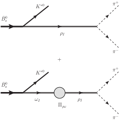
Figure 1: The diagram for the $\bar{B}^{0}_{s}\to{\pi^{+}}{\pi^{-}}K^{*0}$ decay with the $\rho-\omega$ mixing mechanism for the first order of isospin violation in the isospin representation

With the $\rho-\omega$ mixing mechanism, the process of the $\bar{B}^{0}_{s}\to\rho(\omega)K^{*0}\to\pi^{+}\pi^{-}K^{*0}$ decay is shown in Fig.1. In the isospin representation, the decay amplitude $M_{\bar{B}_{s}^{0}}\to\rho(\omega)\to\pi^{+}\pi^{-}$ in Fig.1 can be written as Lu:2013jma ; Guo:1999ip ; Guo:2008zzh ; OConnell:1995nse

$$M_{\bar{B}_{s}^{0}}\to\pi^{+}\pi^{-}=M_{\rho_{I}\to\pi\pi}\frac{1}{s_{\rho}}M_{\bar{B}_{s}^{0}\to\rho_{I}}+M_{\rho_{I}\to\pi\pi}\frac{1}{s_{\rho}}\Pi_{\rho\omega}\frac{1}{s_{\omega}}M_{\bar{B}_{s}^{0}\to\omega_{I}}.$$ (35)

Introducing the $\epsilon=\frac{\Pi_{\rho\omega}}{s_{\rho}-s_{\omega}}$ Lu:2013jma ; Guo:1999ip ; Guo:2008zzh ; OConnell:1995nse , We have identified the physical amplitudes as

$$M_{\rho\to\pi\pi} = M_{\rho_{I}\to\pi\pi},$$ (36)

$$M_{\omega\to\pi\pi} = \epsilon M_{\rho_{I}\to\pi\pi},$$ (37)

$$M_{\bar{B}_{s}^{0}\to\rho} = M_{\bar{B}_{s}^{0}\to\rho_{I}}-\epsilon M_{\bar{B}_{s}^{0}\to\omega_{I}},$$ (38)

$$M_{\bar{B}_{s}^{0}\to\omega} = M_{\bar{B}_{s}^{0}\to\omega_{I}}-\epsilon M_{\bar{B}_{s}^{0}\to\rho_{I}}.$$ (39)

From the physical representation, we can obtain the decay amplitude

$$M_{\bar{B}_{s}^{0}}\to\pi^{+}\pi^{-}=M_{\rho\to\pi\pi}\frac{1}{s_{\rho}}M_{\bar{B}_{s}^{0}\to\rho}+M_{\rho\to\pi\pi}\frac{\Pi_{\rho\omega}s_{\rho}}{s_{\rho}-s_{\omega}}\frac{1}{s_{\rho}s_{\omega}}M_{\bar{B}_{s}^{0}\to\omega_{I}}$$ (40)

where $\mathcal{O}(\epsilon^{2})$ corrections is neglected, and $M_{\rho\to\pi\pi}=g_{\rho}$, $M_{\bar{B}_{s}^{0}\to\rho}$=$t_{\rho}^{i}$ or $p_{\rho}^{i}$ and $M_{\bar{B}_{s}^{0}\to\omega}$=$t_{\omega}^{i}$ or $p_{\omega}^{i}$ are used. So, we can get $\widetilde{\Pi}_{\rho\omega}$=$\frac{\Pi_{\rho\omega}s_{\rho}}{s_{\rho}-s_{\omega}}$. $\widetilde{\Pi}_{\rho\omega}$ is the effective $\rho-\omega$ mixing amplitude which also effectively includes the direct coupling $\omega\rightarrow\pi^{+}\pi^{-}$. At the first order of isospin violation, we have the following tree and penguin amplitudes when the invariant mass of $\pi^{+}\pi^{-}$ pair is near the $\omega$ resonance mass Gardner:1997yx ; Guo:1998eg :

$$\big{<}\pi^{+}\pi^{-}K^{*0}|H^{T}|\bar{B}^{0}_{s}\big{>}=\frac{g_{\rho}}{s_{\rho}s_{\omega}}\widetilde{\Pi}_{\rho\omega}t_{\omega}^{i}+\frac{g_{\rho}}{s_{\rho}}t_{\rho}^{i},$$ (41)

$$\big{<}\pi^{+}\pi^{-}K^{*0}|H^{P}|\bar{B}^{0}_{s}\big{>}=\frac{g_{\rho}}{s_{\rho}s_{\omega}}\widetilde{\Pi}_{\rho\omega}p_{\omega}^{i}+\frac{g_{\rho}}{s_{\rho}}p_{\rho}^{i},$$ (42)

where $t_{\rho}^{i}(p_{\rho}^{i})$ and $t_{\omega}^{i}(p_{\omega}^{i})$ are the tree (penguin)-level helicity amplitudes for $\bar{B}_{s}^{0}\rightarrow\rho^{0}K^{*0}$ and $\bar{B}_{s}^{0}\rightarrow\omega K^{*0}$, respectively. The amplitudes $t_{\rho}^{i}$, $t_{\omega}^{i}$, $p_{\rho}^{i}$ and $p_{\omega}^{i}$ can be found in Sec. III.2. $g_{\rho}$ is the coupling constant for the decay process $\rho^{0}\rightarrow\pi^{+}\pi^{-}$. $s_{V}$, $m_{V}$ and $\Gamma_{V}$($V$=$\rho$ or $\omega$) is the inverse propagator, mass and decay width of the vector meson $V$, respectively. $s_{V}$ can be expressed as

$$s_{V}=s-m_{V}^{2}+{\rm{i}}m_{V}\Gamma_{V},$$ (43)

with $\sqrt{s}$ being the invariant masses of the $\pi^{+}\pi^{-}$ pairs. The $\rho-\omega$ mixing parameter $\widetilde{\Pi}_{\rho\omega}(s)={\rm{Re}}\widetilde{\Pi}_{\rho\omega}(m_{\omega}^{2})+{\rm{Im}}\widetilde{\Pi}_{\rho\omega}(m_{\omega}^{2})$ are Lu:2018fqe

$${\rm{Re}}\widetilde{\Pi}_{\rho\omega}(m_{\omega}^{2}) = -4760\pm{440}\,\rm{MeV}^{2},$$

$${\rm{Im}}\widetilde{\Pi}_{\rho\omega}(m_{\omega}^{2}) = -6180\pm{3300}\,\textrm{MeV}^{2}.$$ (44)

From Eqs. (29), (31), (41) and (42) one has

$$re^{i\delta_{i}}e^{i\phi}=\frac{\widetilde{\Pi}_{\rho\omega}p_{\omega}^{i}+s_{\omega}p_{\rho}^{i}}{\widetilde{\Pi}_{\rho\omega}t_{\omega}^{i}+s_{\omega}t_{\rho}^{i}},$$ (45)

Defining Enomoto:1996cv ; Enomoto:1997bq

$$\frac{p_{\omega}^{i}}{t_{\rho}^{i}}\equiv r^{\prime}e^{i(\delta^{i}_{q}+\phi)},\quad\frac{t_{\omega}^{i}}{t_{\rho}^{i}}\equiv\alpha e^{i\delta^{i}_{\alpha}},\quad\frac{p_{\rho}^{i}}{p_{\omega}^{i}}\equiv\beta e^{i\delta^{i}_{\beta}},$$ (46)

where $\delta^{i}_{\alpha}$, $\delta^{i}_{\beta}$ and $\delta^{i}_{q}$ are strong phases of the decay process $\bar{B}_{s}^{0}\to\rho^{0}(\omega)K^{*0}\to{\pi^{+}}{\pi^{-}}K^{*0}$ from the three kinds of polarizations, respectively. One finds the following expression from Eqs. (45) and (46):

$$re^{i\delta_{i}}=r^{\prime}e^{i\delta^{i}_{q}}\frac{\widetilde{\Pi}_{\rho\omega}+\beta e^{i\delta^{i}_{\beta}}s_{\omega}}{\widetilde{\Pi}_{\rho\omega}\alpha e^{i\delta^{i}_{\alpha}}+s_{\omega}}.$$ (47)

$\alpha e^{i\delta^{i}_{\alpha}}$, $\beta e^{i\delta^{i}_{\beta}}$, and $r^{\prime}e^{i\delta^{i}_{q}}$ will be calculated in the perturbative QCD approach. In order to obtain the $CP$ violating asymmetry in Eq. (34), $A_{CP}$, sin$\phi$ and cos$\phi$ are needed. $\phi$ is determined by the CKM matrix elements. In the Wolfenstein parametrization Wolfenstein:1964ks , the weak phase $\phi$ comes from $[{V_{tb}}V_{td}^{*}/{V_{ub}}V_{ud}^{*}]$. One has

$${\rm sin}\phi = \frac{\eta}{{\sqrt{{{\left[{\rho\left({1-\rho}\right)-{\eta^{2}}}\right]}^{2}}+{\eta^{2}}}}},$$ (48)

$${\rm cos}\phi = \frac{{\rho\left({1-\rho}\right)-{\eta^{2}}}}{{\sqrt{{{\left[{\rho\left({1-\rho}\right)-{\eta^{2}}}\right]}^{2}}+{\eta^{2}}}}},\vspace{2mm}$$ (49)

where the same result has been used for $b\to d$ transition from Ref. Ajaltouni:2003yt ; Leitner:2002xh .

III.2 Calculation details

We can decompose the decay amplitudes for the decay processes $\bar{B}_{s}^{0}\rightarrow\rho^{0}(\omega)K^{*0}$ in terms of tree and penguin contributions depending on the CKM matrix elements of $V_{ub}V^{*}_{ud}$ and $V_{tb}V^{*}_{td}$. From Eqs. (34), (45) and (46), in leading order to obtain the formulas of the $CP$ violation, we need calculate the amplitudes $t_{\rho}$, $p_{\rho}$, $t_{\omega}$ and $p_{\omega}$ in perturbative QCD approach. The relevant function can be found in the Appendix from the perturbative QCD approach.

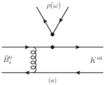
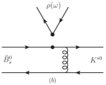
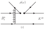
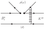
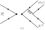
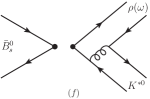
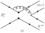
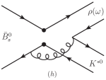
Figure 2: Leading order Feynman diagrams for $\bar{B}_{s}^{0}\to\rho^{0}(\omega)K^{*0}$

In the pQCD, there are eight types of the leading order Feynman diagrams contributing to $\bar{B}_{s}^{0}\rightarrow\rho^{0}(\omega)K^{*0}$ decays, which are shown in Fig.2. The first row is for the emission-type diagrams, where the first two diagrams in Fig.2 (a)(b) are called factorizable emission diagrams and the last two diagrams in Fig.2 (c)(d) are called non-factorizable emission diagrams Zhu:2005rx ; Chen:2002pz . The second row is for the annihilation-type diagrams, where the first two diagrams in Fig.2 (e)(f) are called factorizable annihilation diagrams and the last two diagrams in Fig.2 (g)(h) are called non-factorizable annihilation diagrams Shen:2006ms ; Wang:2014mua . The relevant decay amplitudes can be easily obtained by these hard gluon exchange diagrams and the Lorenz structures of the mesons wave functions. Through calculating these diagrams, the formulas of $\bar{B}_{s}^{0}\to\rho K^{*0}$ or $\bar{B}_{s}^{0}\to\omega K^{*0}$ are similar to those of $B\to\phi K^{*}$ and $B_{s}\to K^{*-}K^{*+}$ Chen:2002pz ; Zou:2015iwa . We just need to replace some corresponding Wilson coefficients, wave functions and corresponding parameters.

With the Hamiltonian equation (1), depending on CKM matrix elements of $V_{ub}V^{*}_{ud}$ and $V_{tb}V^{*}_{td}$, the tree dominant decay amplitudes $A^{(i)}$ for $\bar{B}_{s}^{0}\rightarrow\rho K^{*0}$ in pQCD can be written as

$$\sqrt{2}A^{(i)}(\bar{B}_{s}^{0}\to\rho^{0}K^{*0}) = V_{ub}V_{ud}^{*}T_{\rho}^{i}-V_{tb}V_{td}^{*}P_{\rho}^{i},$$ (50)

where the superscript $i$ denote different helicity amplitudes $L,N$ and $T$. The longitudinal $t_{\rho(\omega)}^{0}$, transverse $t_{\rho(\omega)}^{\pm}$ of helicity amplitudes satisfy relationship from Eq. (27). The amplitudes of the tree and penguin diagrams can be written as $T_{\rho}^{i}=t_{\rho}^{i}/{V_{ub}}V_{ud}^{*}$ and $P_{\rho}^{i}=p_{\rho}^{i}/{V_{tb}}V_{td}^{*}$, respectively. The formula for the tree level amplitude is

$$T_{\rho}^{i}=\frac{G_{F}}{\sqrt{2}}\Big{\{}f_{\rho}F_{B_{s}\to K^{*}}^{LL,i}\left[a_{2}\right]+M_{B_{s}\to K^{*}}^{LL,i}\left[C_{2}\right]\Big{\}},$$ (51)

where $f_{\rho}$ refers to the decay constant of $\rho$ meson. The penguin level amplitude are expressed in the following

$$P_{\rho}^{i} = -\frac{G_{F}}{\sqrt{2}}\Big{\{}f_{\rho}F_{B_{s}\to K^{*}}^{LL,i}\left[-a_{4}+\frac{3}{2}a_{7}+\frac{3}{2}a_{9}+\frac{1}{2}a_{10}\right]-M_{B_{s}\to K^{*}}^{LR,i}\left[-C_{5}+\frac{1}{2}C_{7}\right]$$ (52)

$$+M_{B_{s}\to K^{*}}^{LL,i}\left[-C_{3}+\frac{1}{2}C_{9}+\frac{3}{2}C_{10}\right]-M_{B_{s}\to K^{*}}^{SP,i}\left[\frac{3}{2}C_{8}\right]+f_{B_{s}}F_{ann}^{LL,i}\left[-a_{4}+\frac{1}{2}a_{10}\right]$$

$$-f_{B_{s}}F_{ann}^{SP,i}\left[-a_{6}+\frac{1}{2}a_{8}\right]+M_{ann}^{LL,i}\left[-C_{3}+\frac{1}{2}C_{9}\right]-M_{ann}^{LR,i}\left[-C_{5}+\frac{1}{2}C_{7}\right]\bigg{\}}.$$

The tree dominant decay amplitude for $\bar{B}_{s}^{0}\to\omega K^{*0}$ can be written as

$$\sqrt{2}A^{i}(\bar{B}_{s}^{0}\to\omega K^{*0})=V_{ub}V_{ud}^{*}T_{\omega}^{i}-V_{tb}V_{td}^{*}P_{\omega}^{i},$$ (53)

where $T_{\omega}^{i}=t_{\omega}^{i}/{V_{ub}}V_{us}^{*}$ and $P_{\omega}^{i}=p_{\omega}^{i}/{V_{tb}}V_{ts}^{*}$ which refer to the tree and penguin amplitude, respectively. We can give the tree level contribution in the following

$$T_{\omega}^{i}=\frac{G_{F}}{\sqrt{2}}\Big{\{}f_{\omega}F_{B_{s}\to K^{*}}^{LL,i}\left[a_{2}\right]+M_{B_{s}\to K^{*}}^{LL,i}\left[C_{2}\right]\Big{\}},$$ (54)

where $f_{\omega}$ refers to the decay constant of $\omega$ meson. The penguin level contribution are given as following

$$P_{\omega}^{i} = \frac{G_{F}}{\sqrt{2}}\bigg{\{}f_{\omega}F_{B_{s}\to K^{*}}^{LL,i}\left[2a_{3}+a_{4}+2a_{5}+\frac{1}{2}a_{7}+\frac{1}{2}a_{9}-\frac{1}{2}a_{10}\right]-M_{B_{s}\to K^{*}}^{LR,i}\left[C_{5}-\frac{1}{2}C_{7}\right]$$ (55)

$$+M_{B_{s}\to K^{*}}^{LL,i}\left[C_{3}+2C_{4}-\frac{1}{2}C_{9}+\frac{1}{2}C_{10}\right]-M_{B_{s}\to K^{*}}^{SP,i}\left[2C_{6}+\frac{1}{2}C_{8}\right]+f_{B_{s}}F_{ann}^{LL,i}\left[a_{4}-\frac{1}{2}a_{10}\right]$$

$$-f_{B_{s}}F_{ann}^{SP,i}\left[a_{6}-\frac{1}{2}a_{8}\right]+M_{ann}^{LL,i}\left[C_{3}-\frac{1}{2}C_{9}\right]-M_{ann}^{LR,i}\left[C_{5}-\frac{1}{2}C_{7}\right]\bigg{\}}$$

Based on the definition of Eq. (46), we can get

$$\alpha e^{i\delta^{i}_{\alpha}} = \frac{t_{\omega}^{i}}{t_{\rho}^{i}},$$ (56)

$$\beta e^{i\delta^{i}_{\beta}} = \frac{p_{\rho}^{i}}{p_{\omega}^{i}},$$ (57)

$$r^{\prime}e^{i\delta^{i}_{q}} = \frac{P^{i}_{\omega}}{T^{i}_{\rho}}\times\bigg{|}\frac{V_{tb}V_{td}^{*}}{V_{ub}V_{ud}^{*}}\bigg{|},$$ (58)

where

$$\left|\frac{V_{tb}V^{*}_{td}}{V_{ub}V^{*}_{ud}}\right|=\frac{{\sqrt{{{\left[{\rho\left({1-\rho}\right)-{\eta^{2}}}\right]}^{2}}+{\eta^{2}}}}}{{\left({1-{\lambda^{2}}/2}\right)\left({{\rho^{2}}+{\eta^{2}}}\right)}}.\vspace{2mm}$$ (59)

From above equations, the new strong phases ${\delta^{i}_{\alpha}}$, $\delta^{i}_{\beta}$ and $\delta^{i}_{q}$ are obtained from tree and penguin diagram contributions by the $\rho-\omega$ interference. Substituting Eqs. (56), (57) and (58) into (47), we can obtain total strong phase $\delta_{i}$ in the framework of pQCD. Then in combination with Eqs. (48) and (49) the $CP$ violating asymmetry can be obtained.

IV BRANCHING RATIO OF $\bar{B}^{0}_{s}\rightarrow\rho^{0}(\omega)K^{*0}$

Based on the relationship of Eqs. (24) and (28), we can calculate the decay rates for the processes of $\bar{B}_{s}^{0}\to\rho^{0}(\omega)K^{*0}$ by using the following expression:

$$\Gamma=\frac{{{P_{c}}}}{{8\pi M_{{B_{s}}}^{2}}}(|H_{0}|^{2}+|H_{+}|^{2}+|H_{-}|^{2}),$$ (60)

where

$$P_{c}=\frac{\sqrt{[M_{B_{s}}-(M_{\rho/\omega}+M_{K^{*0}})^{2}][M_{B_{s}}-(M_{\rho/\omega}-M_{K^{*0}})^{2}]}}{2M_{B_{s}}}$$ (61)

is the c.m. momentum of the product particle and $H_{i}(i=0,+,-)$ are helicity amplitudes.

In this case we take into account the $\rho-\omega$ mixing contribution to the branching ratio, since we are working to the first order of isospin violation. The derivation is straightforward and we can explicitly express the branching ratio for the processes $\bar{B}_{s}^{0}\to\rho^{0}(\omega)K^{*0}$ Leitner:2002xh ; Lu:2013xea :

$$BR(\bar{B}_{s}^{0}\to\rho^{0}(\omega)K^{*0})=\frac{\tau_{B^{0}_{s}}P_{c}}{{8\pi M_{{B_{s}}}^{2}}}(|H_{\rho\omega 0}|^{2}+|H_{\rho\omega+}|^{2}+|H_{\rho\omega-}|^{2}),$$ (62)

where $\tau_{B^{0}_{s}}$ is the lifetime of the $B_{s}$ meson and

$$H_{\rho\omega i(i=0,+,-)}=(|V_{ub}V_{ud}^{*}|T_{\rho}^{i}-|V_{tb}V_{td}^{*}|P_{\rho}^{i})+(|V_{ub}V_{ud}^{*}|T_{\omega}^{i}-|V_{tb}V_{td}^{*}|P_{\omega}^{i})\frac{\widetilde{\Pi}_{\rho\omega}}{(s_{\rho}-M_{\omega}^{2})+{\rm{i}}M_{\omega}\Gamma_{\omega}}$$ (63)

take into account the helicity amplitudes of the $\rho$ meson and $\omega$ meson contribution involved in the tree and penguin diagrams.

V Input parameters

The CKM matrix, which elements are determined from experiments, can be expressed in terms of the Wolfenstein parameters $A$, $\rho$, $\lambda$ and $\eta$ Wolfenstein:1983yz ; Wolfenstein:1964ks :

$$\left(\begin{array}[]{ccc}1-\frac{1}{2}\lambda^{2}&\lambda&A\lambda^{3}(\rho-\mathrm{i}\eta)\\ -\lambda&1-\frac{1}{2}\lambda^{2}&A\lambda^{2}\\ A\lambda^{3}(1-\rho-\mathrm{i}\eta)&-A\lambda^{2}&1\\ \end{array}\right),$$ (64)

where $\mathcal{O}(\lambda^{4})$ corrections are neglected. The latest values for the parameters in the CKM matrix are Zyla:2020zbs :

$$\lambda=0.22650\pm 0.00048,\quad A=0.790_{-0.012}^{+0.017},$$

$$\bar{\rho}=0.141_{-0.017}^{+0.016},\quad\bar{\eta}=0.357\pm 0.011,$$ (65)

where

$$\bar{\rho}=\rho(1-\frac{\lambda^{2}}{2}),\quad\bar{\eta}=\eta(1-\frac{\lambda^{2}}{2}).$$ (66)

From Eqs. (65) and (66) we have

$$0.127<\rho<0.161,\quad 0.355<\eta<0.378.$$ (67)

Table 1: Input parameters

Parameters	Input data	References
Fermi constant (in $\rm{GeV}^{-2}$)	$G_{F}=1.16638\times 10^{-5}.$	Zyla:2020zbs
	$M_{B^{0}_{s}}=5366.88,~{}\tau_{B^{0}_{s}}=1.515\times 10^{-12}s,$
	$M_{\rho^{0}(770)}=775.26,~{}\Gamma_{\rho^{0}(770)}=149.1,$
Masses and decay widths (in MeV)	$M_{\omega(782)}=782.65,~{}\Gamma_{\omega(782)}=8.49,$	Zyla:2020zbs
	$M_{\pi}=139.57,~{}M_{K*}=895.55.$
	$f_{\rho}=215.6\pm 5.9,~{}f_{\rho}^{T}=165\pm 9,$
Decay constants (in MeV)	$f_{\omega}=196.5\pm 4.8,~{}f_{\omega}^{T}=145\pm 10,$	Straub:2015ica ; Liu:2016rqu ; Ball:2004rg
	$f_{K^{*}}=217\pm 5,~{}f_{K^{*}}^{T}=185\pm 10.$

VI The numerical results of $CP$ violation and Branching ratio

VI.1 $CP$ violation via $\rho-\omega$ mixing in $\bar{B}^{0}_{s}\rightarrow\rho^{0}(\omega)K^{*0}\rightarrow\pi^{+}\pi^{-}K^{*0}$

We have investigated the $CP$ violating asymmetry, $A_{CP}$, for the $\bar{B}^{0}_{s}\rightarrow\rho^{0}(\omega)K^{*0}\rightarrow\pi^{+}\pi^{-}K^{*0}$ of the three-body decay process in the perturbative QCD. The numerical results of the $CP$ violating asymmetry are shown for the $\bar{B}^{0}_{s}\rightarrow\rho^{0}(\omega)K^{*0}\rightarrow\pi^{+}\pi^{-}K^{*0}$ decay process in Fig. 3. It is found that the $CP$ violation can be enhanced via $\rho-\omega$ mixing for the decay channel $\bar{B}^{0}_{s}\rightarrow\rho^{0}(\omega)K^{*0}\rightarrow\pi^{+}\pi^{-}K^{*0}$ when the invariant mass of $\pi^{+}\pi^{-}$ pair is in the vicinity of the $m_{\omega}$ resonance within perturbative QCD scheme.

The $CP$ violating asymmetry depends on the weak phase difference $\phi$ from CKM matrix elements and the strong phase difference $\delta$ in the Eq. (34). The CKM matrix elements, which relate to $\bar{\rho}$, $A$, $\bar{\eta}$ and $\lambda$, are given in Eq. (65). The uncertainties due to the CKM matrix elements are mostly from $\rho$ and $\eta$ since $\lambda$ is well determined. Hence we take the central value of $\lambda=0.226$ in Eq. (67). In the numerical calculations for the $\bar{B}^{0}_{s}\rightarrow\rho^{0}(\omega)K^{*0}\rightarrow\pi^{+}\pi^{-}K^{*0}$ decay process, we use $\rho$, $\eta$ and $\lambda=0.226$ vary among the limiting values. The numerical results are shown from Fig. 3 with the different parameter values of CKM matrix elements. The solid line, dot line and dash line corresponds to the maximum, middle, and minimum CKM matrix element for the decay channel of $\bar{B}^{0}_{s}\rightarrow\rho^{0}(\omega)K^{*0}\rightarrow\pi^{+}\pi^{-}K^{*0}$, respectively. We find the numberical results of the $CP$ violation is not sensitive to the CKM matrix elements for the different values of $\rho$ and $\eta$. In Fig. 3, we show the plot of $CP$ violation as a function of $\sqrt{s}$ in the perturbative QCD. From the figure, one can see the $CP$ violation parameter is dependent on $\sqrt{s}$ and changes rapidly by the $\rho-\omega$ mixing mechanism when the invariant mass of $\pi^{+}\pi^{-}$ pair is in the vicinity of the $m_{\omega}$ resonance. From the numerical results, it is found that the $CP$ violating asymmetry is large and ranges from -$50.19\%$ to $43.02\%$ via the $\rho-\omega$ mixing mechanism for the process. The maximum $CP$ violating parameter can reach -$48.22^{+1.97}_{-2.04}\%$ for the decay channel of $\bar{B}^{0}_{s}\rightarrow\pi^{+}\pi^{-}K^{*0}$ in the case of ($\rho$, $\eta$). This error corresponds to the CKM parameters.

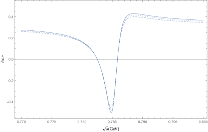
Figure 3: The $CP$ violation, $A_{cp}$, as a function of $\sqrt{s}$ for different CKM matrix elements. The solid line, dot line and dash line corresponds to the maximum, middle, and minimum CKM matrix element for the decay channel of $\bar{B}^{0}_{s}\rightarrow\rho^{0}(\omega)K^{*0}\rightarrow\pi^{+}\pi^{-}K^{*0}$, respectively.

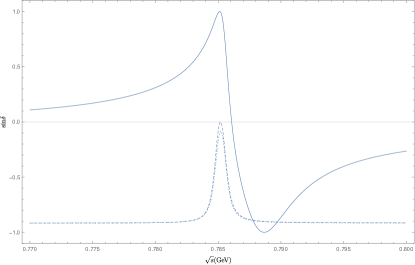
Figure 4: Plot of $\sin\delta$ as a function of $\sqrt{s}$ corresponding to central parameter values of CKM matrix elements for $\bar{B}^{0}_{s}\rightarrow\rho^{0}(\omega)K^{*0}\rightarrow\pi^{+}\pi^{-}K^{*0}$. The solid line, dot line and dash line corresponds to $\sin{\delta_{0}}$, $\sin{\delta_{+}}$ and $\sin{\delta_{-}}$, respectively.

From Eq. (34), one can find that the $CP$ violating parameter is related to $r$ and sin$\delta$. In Fig. 4 and Fig. 5, we show the plots of $\sin\delta_{0}$ ($\sin\delta_{+}$ and $\sin\delta_{-}$) and $r_{0}$ ($r_{+}$ and $r_{-}$) as a function of $\sqrt{s}$, respectively. We can see that the $\rho-\omega$ mixing mechanism produces a large $\sin\delta_{0}$ ($\sin\delta_{+}$ and $\sin\delta_{-}$) in the vicinity of the $\omega$ resonance. As can be seen from Fig. 4, the plots vary sharply in the cases of $\sin\delta_{0}$, $\sin\delta_{+}$ and $\sin\delta_{-}$ in the range of the resonance. Meanwhile, $\sin\delta_{+}$ and $\sin\delta_{-}$ change weakly compared with the $\sin\delta_{0}$. It can be seen from Fig. 5 that $r_{0}$, $r_{+}$ and $r_{-}$ change more rapidly when the $\pi^{+}\pi^{-}$ pairs in the vicinity of the $\omega$ resonance.

We have shown that the $\rho-\omega$ mixing does enhance the direct $CP$ violating asymmetry and provide a mechanism for large $CP$ violation in the perturbative QCD factorization scheme. In other words, it is important to see whether it is possible to observe this large $CP$ violating asymmetry in experiments. This depends on the branching ratio for the decay channel of $\bar{B}^{0}_{s}\rightarrow\rho^{0}K^{*0}$. We will study this problem in the next section.

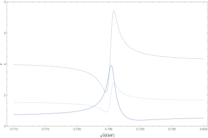
Figure 5: Plot of $r$ as a function of $\sqrt{s}$ corresponding to central parameter values of CKM matrix elements for $\bar{B}^{0}_{s}\rightarrow\rho^{0}(\omega)K^{*0}\rightarrow\pi^{+}\pi^{-}K^{*0}$. The solid line, dot line and dash line corresponds to $r_{0}$, $r_{+}$ and $r_{-}$, respectively.

VI.2 Branching ratio via $\rho-\omega$ mixing in $\bar{B}^{0}_{s}\rightarrow\rho^{0}(\omega)K^{*0}$

Figure 6: The branching ratio, $BR(\bar{B}_{s}^{0}\to\rho(\omega)K^{*0})$, as a function of $\sqrt{s}$ for different CKM matrix elements. The solid line, dot line and dash line corresponds to the maximum, middle, and minimum CKM matrix element for the decay channel of $\bar{B}^{0}_{s}\rightarrow\rho^{0}(\omega)K^{*0}$, respectively.

In the pQCD, we calculate the value of the branching ratio via $\rho-\omega$ mixing mechanism for the decay channel $\bar{B}^{0}_{s}\rightarrow\rho^{0}(\omega)K^{*0}$. The numerical result is shown for the decay process in Fig. 6. Based on a reasonable parameter range, we obtain the maximum branching ratio of $\bar{B}^{0}_{s}\rightarrow\rho^{0}(\omega)K^{*0}$ as ($3.05^{+0.25}_{-0.20}$)$\times 10^{-7}$, which is consistent with the result in Zou:2015iwa ; Yan:2018fif . The error comes from CKM parameters. On the other hand, although we calculate the branching ratio due to $\rho-\omega$ mixing in the pQCD factorization scheme, we find that the contribution of $\rho-\omega$ mixing to the branching ratio of $\bar{B}^{0}_{s}\rightarrow\rho^{0}(\omega)K^{*0}$ is small and can be neglected. However, the $\rho-\omega$ mixing mechanism produces new strong phase differences. This is why the Fig. 6 presents a tiny effect for the branching ratio of $\bar{B}_{s}^{0}\to\rho^{0}(\omega)K^{*0}$ when the invariant mass of $\pi^{+}\pi^{-}$ pair is around 1.1 GeV.

The Large Hadron Collider (LHC) is a proton-proton collider that has started at the European Organization for Nuclear Research (CERN). With the designed center-of-mass energy 14 TeV and luminosity $L=10^{34}\text{cm}^{-2}\text{s}^{-1}$, the LHC provides a high energy frontier at TeV-level scale and an opportunity to further improve the consistency test for the CKM matrix. LHCb is a dedicated heavy flavor physics experiments and one of the main projects of LHC. Its main goal is to search for indirect evidence of new physics in $CP$ violation and rare decays in the interactions of beauty and charm hadrons systems, by looking for the effects of new particles in decay processes that are precisely predicted in the SM. Such studies can help us to comprehend the matter-antimatter asymmetry of the universe. Recently, the LHCb collaboration found clear evidence for direct $CP$ violation in some three-body decay channels of $B$ meson. Large $CP$ violation is obtained for the decay channels of $B^{\pm}\rightarrow\pi^{\pm}\pi^{+}\pi^{-}$ in the localized phase spaces region $m^{2}_{\pi^{+}\pi^{-}\text{low}}<0.4$ GeV² and $m^{2}_{\pi^{+}\pi^{-}\text{high}}>15$ GeV² Aaij:2013bla ; dosReis:2016ayt . A zoom of the $\pi^{+}\pi^{-}$ invariant mass from the $B^{+}\rightarrow\pi^{+}\pi^{+}\pi^{-}$ decay process is shown the region $m^{2}_{\pi^{+}\pi^{-}low}<1$ GeV² zone in the Ref. dosReis:2016ayt . In addition, the branching ratio of $\bar{B}^{0}_{s}\rightarrow\pi^{+}\pi^{-}\phi$ is probed in the $\pi^{+}\pi^{-}$ invariant mass range $400<m({\pi^{+}}{\pi^{-}})<1600$ MeV/$\rm{c^{2}}$ Aaij:2016qnm . In the next years, we expect the LHCb Collaboration to collect date for detecting our prediction of $CP$ violation from the $\bar{B}^{0}_{s}\rightarrow\rho^{0}(\omega)K^{*0}\rightarrow\pi^{+}\pi^{-}K^{*0}$ decay process when the invariant mass of $\pi^{+}\pi^{-}$ is in the vicinity of the $\omega$ resonance.

At the LHC, the $b$-hadrons come from $pp$ collisions. The possible asymmetry between the numbers of the $b$-hadrons $H_{b}$ and those of their anti-particles $\bar{H}_{b}$ has been studied by using the intrinsic heavy quark model and the Lund string fragmentation model Norrbin:1999by ; Altarelli:2000ye . It has been shown that this asymmetry can only reach values of a few percents. In the following discussion, we will ignore this small asymmetry and give the numbers of $H_{b}\bar{H}_{b}$ pairs needed for observing our prediction of the $CP$ violating asymmetries. These numbers depend on both the magnitudes of the $CP$ violating asymmetries and the branching ratios of heavy hadron decays which are model dependent. For one-standard-deviation (1$\sigma$) signature and three-standard deviation (3$\sigma$) signature, the numbers of $H_{b}\bar{H}_{b}$ pairs we need Du:1986ai ; Eadie:1971qcl ; Lyons:1986em

$$N_{H_{b}\bar{H}_{b}}(1\sigma)\sim\frac{1}{BR(\bar{B}_{s}^{0}\rightarrow\rho^{0}K^{*0})A_{CP}^{2}}(1-A_{CP}^{2})$$ (68)

and

$$N_{H_{b}\bar{H}_{b}}(3\sigma)\sim\frac{9}{BR(\bar{B}_{s}^{0}\rightarrow\rho^{0}K^{*0})A_{CP}^{2}}(1-A_{CP}^{2}),$$ (69)

where $A_{CP}$ is the $CP$ violation in the process of $\bar{B}^{0}_{s}\rightarrow\rho^{0}(\omega)K^{*0}\rightarrow\pi^{+}\pi^{-}K^{*0}$. Now, we can estimate the possibility to observe $CP$ violation. The branching ratio for $\bar{B}_{s}^{0}\rightarrow\rho^{0}(\omega)K^{*0}$ is of order $10^{-7}$, then the number $N_{H_{b}\bar{H}_{b}}(1\sigma)\sim 10^{6}$ for $1\sigma$ signature and $10^{7}$ for $3\sigma$ signature. Theoretically, in order to achieve the current experiments on $b$-hadrons, which can only provide about $10^{7}$ $B_{s}\bar{B}_{s}$ pairs. Therefore, it is very possible to observe the large $CP$ violation for $\bar{B}^{0}_{s}\rightarrow\rho^{0}(\omega)K^{*0}\rightarrow\pi^{+}\pi^{-}K^{*0}$ when the invariant masses of $\pi^{+}\pi^{-}$ pairs are in the vicinity of the $\omega$ resonance in experiments at the LHC.

VII Summary and conclusion

In this paper, we have studied the direct $CP$ violation for the decay process of $\bar{B}^{0}_{s}\rightarrow\rho^{0}(\omega)K^{*0}\rightarrow\pi^{+}\pi^{-}K^{*0}$ in perturbative QCD. It has been found that, by using $\rho-\omega$ mixing, the $CP$ violation can be enhanced at the area of $\omega$ resonance. There is the resonance effect via $\rho-\omega$ mixing which can produce large strong phase in this decay process. As a result, one can find that the maximum $CP$ violation can reach -$50.19\%$ when the invariant mass of the $\pi^{+}\pi^{-}$ pair is in the vicinity of the $\omega$ resonance. Furthermore, taking $\rho-\omega$ mixing into account, we have calculated the branching ratio of the decays of $\bar{B}^{0}_{s}\rightarrow\rho^{0}(\omega)K^{*0}$. We have also given the numbers of $B_{s}\bar{B}_{s}$ pairs required for observing our prediction of the $CP$ violating asymmetries at the LHC experiments.

In our calculation there are some uncertainties. The major uncertainties come from the input parameters. In particular, these include the CKM matrix element, the particle mass, the perturbative QCD approach and the hadronic parameters (decay constants, the wave functions, the shape parameters and etc). We expect that our predictions will provide useful guidance for future experiments.

Appendix: Related functions defined in the text

In this appendix we present explicit expressions of the factorizable and non-factorizable amplitudes in Perturbative QCD Ali:2007ff ; Keum:2000ph ; Keum:2000wi ; Lu:2000em . The factorizable amplitudes $F_{B_{s}\to K^{*}}^{LL,i}(a_{i})$, $F_{ann}^{LL,i}(a_{i})$ and $F_{ann}^{SP,i}(a_{i})$ (i=L,N,T) are written as

$$f_{M_{2}}F^{LL,L}_{B_{s}\to K^{*}}(a_{i}) = 8\pi C_{F}M_{B_{s}}^{4}f_{M_{2}}\int^{1}_{0}dx_{1}dx_{3}\int^{\infty}_{0}b_{1}db_{1}b_{3}db_{3}\phi_{B_{s}}(x_{1},b_{1})\Big{\{}a_{i}(t_{a})E_{e}(t_{a})$$ (70)

$$\times\left[r_{3}(1-2x_{3})(\phi_{3}^{s}(x_{3})+\phi_{3}^{t}(x_{3}))+(1+x_{3})\phi_{3}(x_{3})\right]h_{e}(x_{1},x_{3},b_{1},b_{3})$$

$$+2r_{3}\phi_{3}^{s}(x_{3})a_{i}(t_{a}^{\prime})E_{e}(t_{a}^{\prime})h_{e}(x_{3},x_{1},b_{3},b_{1})\Big{\}},$$

$$f_{M_{2}}F^{LL,N}_{B_{s}\to K^{*}}(a_{i}) = 8\pi C_{F}M_{B_{s}}^{4}f_{M_{2}}r_{2}\int^{1}_{0}dx_{1}dx_{3}\int^{\infty}_{0}b_{1}db_{1}b_{3}db_{3}\phi_{B_{s}}(x_{1},b_{1})\Big{\{}h_{e}(x_{1},x_{3},b_{1},b_{3})$$ (71)

$$\times E_{e}(t_{a})a_{i}(t_{a})\left[2r_{3}\phi_{3}^{v}(x_{3})+r_{3}x_{3}(\phi_{3}^{v}(x_{3})-\phi_{3}^{a}(x_{3}))+\phi_{3}^{T}(x_{3})\right]$$

$$+r_{3}\left[\phi_{3}^{v}(x_{3})+\phi_{3}^{a}(x_{3})\right]E_{e}(t_{a}^{\prime})a_{i}(t_{a}^{\prime})h_{e}(x_{3},x_{1},b_{3},b_{1})\Big{\}},$$

$$f_{M_{2}}F^{LL,T}_{B_{s}\to K^{*}}(a_{i}) = 16\pi C_{F}M_{B_{s}}^{4}f_{M_{2}}r_{2}\int^{1}_{0}dx_{1}dx_{3}\int^{\infty}_{0}b_{1}db_{1}b_{3}db_{3}\phi_{B_{s}}(x_{1},b_{1})\Big{\{}h_{e}(x_{1},x_{3},b_{1},b_{3})$$ (72)

$$\times\left[2r_{3}\phi_{3}^{v}(x_{3})-r_{3}x_{3}(\phi_{3}^{v}(x_{3})-\phi_{3}^{a}(x_{3}))+\phi_{3}^{T}(x_{3})\right]E_{e}(t_{a})a_{i}(t_{a})$$

$$+r_{3}\left[\phi_{3}^{v}(x_{3})+\phi_{3}^{a}(x_{3})\right]E_{e}(t_{a}^{\prime})a_{i}(t_{a}^{\prime})h_{e}(x_{3},x_{1},b_{3},b_{1})\Big{\}},$$

$$f_{B_{s}}F_{ann}^{LL,L}(a_{i}) = 8\pi C_{F}M_{B_{s}}^{4}f_{B_{s}}\int^{1}_{0}dx_{2}dx_{3}\int^{\infty}_{0}b_{2}db_{2}b_{3}db_{3}\Big{\{}a_{i}(t_{c})E_{a}(t_{c})[(x_{3}-1)\phi_{2}(x_{2})\phi_{3}(x_{3})$$ (73)

$$-4r_{2}r_{3}\phi_{2}^{s}(x_{2})\phi_{3}^{s}(x_{3})+2r_{2}r_{3}x_{3}\phi_{2}^{s}(x_{2})(\phi_{3}^{s}(x_{3})-\phi_{3}^{t}(x_{3}))]h_{a}(x_{2},1-x_{3},b_{2},b_{3})$$

$$+[x_{2}\phi_{2}(x_{2})\phi_{3}(x_{3})+2r_{2}r_{3}(\phi_{2}^{s}(x_{2})-\phi_{2}^{t}(x_{2}))\phi_{3}^{s}(x_{3})+2r_{2}r_{3}x_{2}(\phi_{2}^{s}(x_{2})$$

$$+\phi_{2}^{t}(x_{2}))\phi_{3}^{s}(x_{3})]a_{i}(t_{c}^{\prime})E_{a}(t_{c}^{\prime})h_{a}(1-x_{3},x_{2},b_{3},b_{2})\Big{\}},$$

$$f_{B_{s}}F_{ann}^{LL,N}(a_{i}) = -8\pi C_{F}M_{B_{s}}^{4}f_{B_{s}}r_{2}r_{3}\int^{1}_{0}dx_{2}dx_{3}\int^{\infty}_{0}b_{2}db_{2}b_{3}db_{3}\Big{\{}E_{a}(t_{c})a_{i}(t_{c})h_{a}(x_{2},1-x_{3},b_{2},b_{3}))$$ (74)

$$\times\left[x_{3}(\phi_{2}^{v}(x_{2})\phi_{3}^{a}(x_{3})+\phi_{2}^{a}(x_{2})\phi_{3}^{v}(x_{3}))+(2-x_{3})\left(\phi_{2}^{v}(x_{2})\phi_{3}^{v}(x_{3})+\phi_{2}^{a}(x_{2})\phi_{3}^{a}(x_{3})\right)\right]$$

$$-h_{a}(1-x_{3},x_{2},b_{3},b_{2})[(1+x_{2})(\phi_{2}^{a}(x_{2})\phi_{3}^{a}(x_{3})+\phi_{2}^{v}(x_{2})\phi_{3}^{v}(x_{3}))$$

$$-(1-x_{2})(\phi_{2}^{a}(x_{2})\phi_{3}^{v}(x_{3}))+\phi_{2}^{v}(x_{2})\phi_{3}^{a}(x_{3})]E_{a}(t_{c}^{\prime})a_{i}(t_{c}^{\prime})\Big{\}},$$

$$f_{B_{s}}F_{ann}^{LL,T}(a_{i}) = -16\pi C_{F}M_{B_{s}}^{4}f_{B_{s}}r_{2}r_{3}\int^{1}_{0}dx_{2}dx_{3}\int^{\infty}_{0}b_{2}db_{2}b_{3}db_{3}\Big{\{}\Big{[}x_{3}(\phi_{2}^{a}(x_{2})\phi_{3}^{a}(x_{3})+\phi_{2}^{v}(x_{2})\phi_{3}^{v}(x_{3}))$$ (75)

$$+(2-x_{3})(\phi_{2}^{a}(x_{2})\phi_{3}^{v}(x_{3})+\phi_{2}^{v}(x_{2})\phi_{3}^{a}(x_{3}))\Big{]}E_{a}(t_{c})a_{i}(t_{c})h_{a}(x_{2},1-x_{3},b_{2},b_{3})$$

$$+h_{a}(1-x_{3},x_{2},b_{3},b_{2})[(1-x_{2})(\phi_{2}^{a}(x_{2})\phi_{3}^{a}(x_{3})+\phi_{2}^{v}(x_{2})\phi_{3}^{v}(x_{3}))$$

$$-(1+x_{2})(\phi_{2}^{a}(x_{2})\phi_{3}^{v}(x_{3})+\phi_{2}^{v}(x_{2})\phi_{3}^{a}(x_{3}))]E_{a}(t_{c}^{\prime})a_{i}(t_{c}^{\prime})\Big{\}},$$

$$f_{B_{s}}F_{ann}^{SP,L}(a_{i}) = 16\pi C_{F}M_{B_{s}}^{4}f_{B_{s}}\int^{1}_{0}dx_{2}dx_{3}\int^{\infty}_{0}b_{2}db_{2}b_{3}db_{3}\Big{\{}[(x_{3}-1)r_{3}\phi_{2}(x_{2})(\phi_{3}^{s}(x_{3})+\phi_{3}^{t}(x_{3}))$$ (76)

$$-2r_{2}\phi_{2}^{s}(x_{2})\phi_{3}(x_{3})]a_{i}(t_{c})E_{a}(t_{c})h_{a}(x_{2},1-x_{3},b_{2},b_{3})-[2r_{3}\phi_{2}(x_{2})\phi_{3}^{s}(x_{3})$$

$$+r_{2}x_{2}(\phi_{2}^{s}(x_{2})-\phi_{2}^{t}(x_{2}))\phi_{3}(x_{3})]a_{i}(t_{c}^{\prime})E_{a}(t_{c}^{\prime})h_{a}(1-x_{3},x_{2},b_{3},b_{2})\Big{\}},$$

$$f_{B_{s}}F_{ann}^{SP,T}(a_{i}) = 2f_{B_{s}}F_{ann}^{SP,N}(a_{i})$$ (77)

$$= -32\pi C_{F}M_{B_{s}}^{4}f_{B_{s}}\int^{1}_{0}dx_{2}dx_{3}\int^{\infty}_{0}b_{2}db_{2}b_{3}db_{3}\Big{\{}r_{2}(\phi_{2}^{a}(x_{2})+\phi_{2}^{v}(x_{2}))\phi_{3}^{T}(x_{3})$$

$$\times E_{a}(t_{c})a_{i}(t_{c})h_{a}(x_{2},1-x_{3},b_{2},b_{3})+r_{3}\phi_{2}^{T}(x_{2})$$

$$\times(\phi_{3}^{v}(x_{3})-\phi_{3}^{a}(x_{3}))E_{a}(t_{c}^{\prime})a_{i}(t_{c}^{\prime})h_{a}(1-x_{3},x_{2},b_{3},b_{2})\Big{\}},$$

with the color factor ${C_{F}}=3/4$, $a_{i}$ represents the corresponding Wilson coefficients for specific decay channels and $f_{M_{2}}$, $f_{B_{s}}$ refer to the decay constants of $M_{2}$ ($\rho$ or $\omega)$ and $\bar{B}_{s}^{0}$ mesons. In the above functions, $r_{2}(r_{3})=M_{V_{2}}(M_{V_{3}})/M_{B_{s}}$ and $\phi_{2}(\phi_{3})=\phi_{\rho/\omega}(\phi_{K^{*}})$, with $M_{B_{s}}$ and $M_{V_{2}}(m_{V_{3}})$ being the masses of the initial and final states.

The non-factorizable amplitudes $M_{B_{s}\to K^{*}}^{LL,i}(a_{i})$, $M_{B_{s}\to K^{*}}^{LR,i}(a_{i})$, $M_{B_{s}\to K^{*}}^{SP,i}(a_{i})$, $M_{ann}^{LL,i}(a_{i})$ and $M_{ann}^{LR,i}(a_{i})$(i=L,N,T) are written as

$$M_{B_{s}\to K^{*}}^{LL,L}(a_{i}) = 32\pi C_{F}M_{B_{s}}^{4}/\sqrt{6}\int^{1}_{0}dx_{1}dx_{2}dx_{3}\int^{\infty}_{0}b_{1}db_{1}b_{2}db_{2}\phi_{B_{s}}(x_{1},b_{1})\phi_{2}(x_{2})$$ (78)

$$\times\Big{\{}\Big{[}(1-x_{2})\phi_{3}(x_{3})-r_{3}x_{3}(\phi_{3}^{s}(x_{3})-\phi_{3}^{t}(x_{3}))\Big{]}a_{i}(t_{b})E_{e}^{\prime}(t_{b})$$

$$\times h_{n}(x_{1},1-x_{2},x_{3},b_{1},b_{2})+h_{n}(x_{1},x_{2},x_{3},b_{1},b_{2})$$

$$\times\Big{[}r_{3}x_{3}(\phi_{3}^{s}(x_{3})+\phi_{3}^{t}(x_{3}))-(x_{2}+x_{3})\phi_{3}(x_{3})\Big{]}a_{i}(t_{b}^{\prime})E_{e}^{\prime}(t_{b}^{\prime})\Big{\}},$$

$$M_{B_{s}\to K^{*}}^{LL,N}(a_{i}) = 32\pi C_{F}M_{B_{s}}^{4}r_{2}/\sqrt{6}\int^{1}_{0}dx_{1}dx_{2}dx_{3}\int^{\infty}_{0}b_{1}db_{1}b_{2}db_{2}\phi_{B_{s}}(x_{1},b_{1})$$ (79)

$$\times\Big{\{}\left[x_{2}(\phi_{2}^{v}(x_{2})+\phi_{2}^{a}(x_{2}))\phi_{3}^{T}(x_{3})-2r_{3}(x_{2}+x_{3})(\phi_{2}^{a}(x_{2})\phi_{3}^{a}(x_{3})+\phi_{2}^{v}(x_{2})\phi_{3}^{v}(x_{3}))\right]$$

$$\times h_{n}(x_{1},x_{2},x_{3},b_{1},b_{2})E_{e}^{\prime}(t_{b}^{\prime})a_{i}(t_{b}^{\prime})+(1-x_{2})(\phi_{2}^{v}(x_{2})+\phi_{2}^{a}(x_{2}))\phi_{3}^{T}(x_{3})$$

$$\times E_{e}^{\prime}(t_{b})a_{i}(t_{b})h_{n}(x_{1},1-x_{2},x_{3},b_{1},b_{2})\Big{\}},$$

$$M_{B_{s}\to K^{*}}^{LL,T}(a_{i}) = 64\pi C_{F}M_{B_{s}}^{4}r_{2}/\sqrt{6}\int^{1}_{0}dx_{1}dx_{2}dx_{3}\int^{\infty}_{0}b_{1}db_{1}b_{2}db_{2}\phi_{B_{s}}(x_{1},b_{1})\Big{\{}E_{e}^{\prime}(t_{b}^{\prime})a_{i}(t_{b}^{\prime})$$ (80)

$$\times\big{[}x_{2}(\phi_{2}^{v}(x_{2})+\phi_{2}^{a}(x_{2}))\phi_{3}^{T}(x_{3})-2r_{3}(x_{2}+x_{3})(\phi_{2}^{v}(x_{2})\phi_{3}^{a}(x_{3})$$

$$+\phi_{2}^{a}(x_{2})\phi_{3}^{v}(x_{3}))\big{]}h_{n}(x_{1},x_{2},x_{3},b_{1},b_{2})+(1-x_{2})[\phi_{2}^{v}(x_{2})+\phi_{2}^{a}(x_{2})]\phi_{3}^{T}(x_{3})$$

$$\times E_{e}^{\prime}(t_{b})a_{i}(t_{b})h_{n}(x_{1},1-x_{2},x_{3},b_{1},b_{2})\Big{\}},$$

$$M_{B_{s}\to K^{*}}^{LR,L}(a_{i}) = 32\pi C_{F}M_{B_{s}}^{4}r_{2}/\sqrt{6}\int^{1}_{0}dx_{1}dx_{2}dx_{3}\int^{\infty}_{0}b_{1}db_{1}b_{2}db_{2}\phi_{B_{s}}(x_{1},b_{1})$$ (81)

$$\times\Big{\{}h_{n}(x_{1},1-x_{2},x_{3},b_{1},b_{2})\Big{[}(1-x_{2})\phi_{3}(x_{3})\left(\phi_{2}^{s}(x_{2})+\phi_{2}^{t}(x_{2})\right)$$

$$+r_{3}x_{3}\left(\phi_{2}^{s}(x_{2})-\phi_{2}^{t}(x_{2})\right)\left(\phi_{3}^{s}(x_{3})+\phi_{3}^{t}(x_{3})\right)$$

$$+(1-x_{2})r_{3}\left(\phi_{2}^{s}(x_{2})+\phi_{2}^{t}(x_{2})\right)\left(\phi_{3}^{s}(x_{3})-\phi_{3}^{t}(x_{3})\right)\Big{]}a_{i}(t_{b})E_{e}^{\prime}(t_{b})$$

$$-h_{n}(x_{1},x_{2},x_{3},b_{1},b_{2})\Big{[}x_{2}\phi_{3}(x_{3})(\phi_{2}^{s}(x_{2})-\phi_{2}^{t}(x_{2}))$$

$$+r_{3}x_{2}(\phi_{2}^{s}(x_{2})-\phi_{2}^{t}(x_{2}))(\phi_{3}^{s}(x_{3})-\phi_{3}^{t}(x_{3}))$$

$$+r_{3}x_{3}(\phi_{2}^{s}(x_{2})+\phi_{2}^{t}(x_{2}))(\phi_{3}^{s}(x_{3})+\phi_{3}^{t}(x_{3}))\Big{]}a_{i}(t^{\prime}_{b})E_{e}^{\prime}(t_{b}^{\prime})\Big{\}},$$

$$M_{B_{s}\to K^{*}}^{LR,T}(a_{i}) = 2M_{B_{s}\to K^{*}}^{LR,N}(a_{i})$$ (82)

$$= 64\pi C_{F}M_{B_{s}}^{4}/\sqrt{6}\int^{1}_{0}dx_{1}dx_{2}dx_{3}\int^{\infty}_{0}b_{1}db_{1}b_{2}db_{2}\phi_{B_{s}}(x_{1},b_{1})$$

$$\times r_{3}x_{3}\phi_{2}^{T}(x_{2})(\phi_{3}^{v}(x_{3})-\phi_{3}^{a}(x_{3}))$$

$$\times\Big{\{}E_{e}^{\prime}(t_{b})a_{i}(t_{b})h_{n}(x_{1},1-x_{2},x_{3},b_{1},b_{2})+E_{e}^{\prime}(t_{b}^{\prime})a_{i}(t_{b}^{\prime})h_{n}(x_{1},x_{2},x_{3},b_{1},b_{2})\Big{\}},$$

$$M^{SP,L}_{B_{s}\to K^{*}}(a_{i}) = 32\pi C_{F}M_{B_{s}}^{4}/\sqrt{6}\int^{1}_{0}dx_{1}dx_{2}dx_{3}\int^{\infty}_{0}b_{1}db_{1}b_{2}db_{2}\phi_{B_{s}}(x_{1},b_{1})\phi_{2}(x_{2})$$ (83)

$$\times\Big{\{}\Big{[}(x_{2}-x_{3}-1)\phi_{3}(x_{3})+r_{3}x_{3}(\phi_{3}^{s}(x_{3})+\phi_{3}^{t}(x_{3}))\Big{]}$$

$$\times a_{i}(t_{b})E_{e}^{\prime}(t_{b})h_{n}(x_{1},1-x_{2},x_{3},b_{1},b_{2})+a_{i}(t_{b}^{\prime})E^{\prime}_{e}(t_{b}^{\prime})$$

$$\times\Big{[}x_{2}\phi_{3}(x_{3})+r_{3}x_{3}(\phi_{3}^{t}(x_{3})-\phi_{3}^{s}(x_{3}))\Big{]}h_{n}(x_{1},x_{2},x_{3},b_{1},b_{2})\Big{\}},$$

$$M^{SP,N}_{B_{s}\to K^{*}}(a_{i}) = 32\pi C_{F}M_{B_{s}}^{4}/\sqrt{6}\int^{1}_{0}dx_{1}dx_{2}dx_{3}\int^{\infty}_{0}b_{1}db_{1}b_{2}db_{2}\phi_{B_{s}}(x_{1},b_{1})r_{2}$$ (84)

$$\times\Big{\{}x_{2}(\phi_{2}^{v}(x_{2})-\phi_{2}^{a}(x_{2}))\phi_{3}^{T}(x_{3})E_{e}^{\prime}(t_{b}^{\prime})a_{i}(t_{b}^{\prime})h_{n}(x_{1},x_{2},x_{3},b_{1},b_{2})$$

$$+h_{n}(x_{1},1-x_{2},x_{3},b_{1},b_{2})[(1-x_{2})(\phi_{2}^{v}(x_{2})-\phi_{2}^{a}(x_{2}))\phi_{3}^{T}(x_{3})$$

$$-2r_{3}(1-x_{2}+x_{3})(\phi_{2}^{v}(x_{2})\phi_{3}^{v}(x_{3})-\phi_{2}^{a}(x_{2})\phi_{3}^{a}(x_{3}))]E_{e}^{\prime}(t_{b})a_{i}(t_{b})\Big{\}},$$

$$M^{SP,T}_{B_{s}\to K^{*}}(a_{i}) = 64\pi C_{F}M_{B_{s}}^{4}/\sqrt{6}\int^{1}_{0}dx_{1}dx_{2}dx_{3}\int^{\infty}_{0}b_{1}db_{1}b_{2}db_{2}\phi_{B_{s}}(x_{1},b_{1})r_{2}$$ (85)

$$\times\Big{\{}x_{2}(\phi_{2}^{v}(x_{2})-\phi_{2}^{a}(x_{2}))\phi_{3}^{T}(x_{3})E_{e}^{\prime}(t_{b}^{\prime})a_{i}(t_{b}^{\prime})h_{n}(x_{1},x_{2},x_{3},b_{1},b_{2})$$

$$+h_{n}(x_{1},1-x_{2},x_{3},b_{1},b_{2})[(1-x_{2})(\phi_{2}^{v}(x_{2})-\phi_{2}^{a}(x_{2}))\phi_{3}^{T}(x_{3})$$

$$-2r_{3}(1-x_{2}+x_{3})(\phi_{2}^{v}(x_{2})\phi_{3}^{a}(x_{3})-\phi_{2}^{a}(x_{2})\phi_{3}^{v}(x_{3}))]E_{e}^{\prime}(t_{b})a_{i}(t_{b})\Big{\}},$$

$$M_{ann}^{LL,L}(a_{i}) = 32\pi C_{F}M_{B_{s}}^{4}/\sqrt{6}\int^{1}_{0}dx_{1}dx_{2}dx_{3}\int^{\infty}_{0}b_{1}db_{2}b_{2}db_{2}\phi_{B_{s}}(x_{1},b_{1})\Big{\{}h_{na}(x_{1},x_{2},x_{3},b_{1},b_{2})$$ (86)

$$\times\Big{[}r_{2}r_{3}x_{3}(\phi_{2}^{s}(x_{2})-\phi_{2}^{t}(x_{2}))(\phi_{3}^{s}(x_{3})+\phi_{3}^{t}(x_{3}))-(x_{2}\phi_{2}(x_{2})\phi_{3}(x_{3})+4r_{2}r_{3}\phi_{2}^{s}(x_{2})\phi_{3}^{s}(x_{3}))$$

$$+r_{2}r_{3}(1-x_{2})(\phi_{2}^{s}(x_{2})+\phi_{2}^{t}(x_{2}))(\phi_{3}^{s}(x_{3})-\phi_{3}^{t}(x_{3}))\Big{]}a_{i}(t_{d})E_{a}^{\prime}(t_{d})+h_{na}^{\prime}(x_{1},x_{2},x_{3},b_{1},b_{2})$$

$$\times\Big{[}(1-x_{3})\phi_{2}(x_{2})\phi_{3}(x_{3})+(1-x_{3})r_{2}r_{3}(\phi_{2}^{s}(x_{2})+\phi_{2}^{t}(x_{2}))(\phi_{3}^{s}(x_{3})-\phi_{3}^{t}(x_{3}))$$

$$+x_{2}r_{2}r_{3}(\phi_{2}^{s}(x_{2})-\phi_{2}^{t}(x_{2}))(\phi_{3}^{s}(x_{3})+\phi_{3}^{t}(x_{3}))\Big{]}a_{i}(t_{d}^{\prime})E_{a}^{\prime}(t_{d}^{\prime})\Big{\}},$$

$$M_{ann}^{LL,N}(a_{i}) = -64\pi C_{F}M_{B_{s}}^{4}r_{2}r_{3}/\sqrt{6}\int^{1}_{0}dx_{1}dx_{2}dx_{3}\int^{\infty}_{0}b_{1}db_{2}b_{2}db_{2}\phi_{B_{s}}(x_{1},b_{1})[\phi_{2}^{v}(x_{2})\phi_{3}^{v}(x_{3})$$ (87)

$$+\phi_{2}^{a}(x_{2})\phi_{3}^{a}(x_{3})]E_{a}^{\prime}(t_{d})a_{i}(t_{d})h_{na}(x_{1},x_{2},x_{3},b_{1},b_{2}),$$

$$M_{ann}^{LL,T}(a_{i}) = -128\pi C_{F}M_{B_{s}}^{4}r_{2}r_{3}/\sqrt{6}\int^{1}_{0}dx_{1}dx_{2}dx_{3}\int^{\infty}_{0}b_{1}db_{2}b_{2}db_{2}\phi_{B_{s}}(x_{1},b_{1})[\phi_{2}^{v}(x_{2})\phi_{3}^{a}(x_{3})$$ (88)

$$+\phi_{2}^{a}(x_{2})\phi_{3}^{v}(x_{3})]E_{a}^{\prime}(t_{d})a_{i}(t_{d})h_{na}(x_{1},x_{2},x_{3},b_{1},b_{2}),$$

$$M_{ann}^{LR,L}(a_{i}) = 32\pi C_{F}M_{B_{s}}^{4}/\sqrt{6}\int^{1}_{0}dx_{1}dx_{2}dx_{3}\int^{\infty}b_{1}db_{1}b_{2}db_{2}\phi_{B_{s}}(x_{1},b_{1})\Big{\{}h_{na}(x_{1},x_{2},x_{3},b_{1},b_{2})$$ (89)

$$\times\Big{[}r_{2}(x_{2}-2)(\phi_{2}^{s}(x_{2})+\phi_{2}^{t}(x_{2}))\phi_{3}(x_{3})+r_{3}(1+x_{3})\phi_{2}(x_{2})(\phi_{3}^{s}(x_{3})-\phi_{3}^{t}(x_{3}))\Big{]}a_{i}(t_{d})E_{a}^{\prime}(t_{d})$$

$$+h_{na}^{\prime}(x_{1},x_{2},x_{3},b_{1},b_{2})\Big{[}-r_{2}x_{2}\left(\phi_{2}^{s}(x_{2})+\phi_{2}^{t}(x_{2})\right)\phi_{3}(x_{3})$$

$$+r_{3}(1-x_{3})\phi_{2}(x_{2})(\phi_{3}^{s}(x_{3})-\phi_{3}^{t}(x_{3}))\Big{]}a_{i}(t_{d}^{\prime})E_{a}^{\prime}(t_{d}^{\prime})\Big{\}},$$

$$M_{ann}^{LR,T}(a_{i}) = 2M_{ann}^{LR,N}(a_{i})$$ (90)

$$= -64\pi C_{F}M_{B_{s}}^{4}/\sqrt{6}\int^{1}_{0}dx_{1}dx_{2}dx_{3}\int^{\infty}b_{1}db_{1}b_{2}db_{2}\phi_{B_{s}}(x_{1},b_{1})\Big{\{}h_{na}^{\prime}(x_{1},x_{2},x_{3},b_{1},b_{2})$$

$$\times\left[r_{2}x_{2}(\phi_{2}^{v}(x_{2})+\phi_{2}^{a}(x_{2}))\phi_{3}^{T}(x_{3})-r_{3}(1-x_{3})\phi_{2}^{T}(x_{2})(\phi_{3}^{v}(x_{3})-\phi_{3}^{a}(x_{3}))\right]E_{a}^{\prime}(t_{d}^{\prime})a_{i}(t_{d}^{\prime})$$

$$+\left[r_{2}(2-x_{2})(\phi_{2}^{v}(x_{2})+\phi_{2}^{a}(x_{2}))\phi_{3}^{T}(x_{3})-r_{3}(1+x_{3})\phi_{2}^{T}(x_{2})(\phi_{3}^{v}(x_{3})-\phi_{3}^{a}(x_{3}))\right]$$

$$\times E_{a}^{\prime}(t_{d})a_{i}(t_{d})h_{na}(x_{1},x_{2},x_{3},b_{1},b_{2})\Big{\}}.$$

The hard scale t are chosen as the maximum of the virtuality of the internal momentum transition in the hard amplitudes, including $1/b_{i}$:

$$t_{a} = \mbox{max}\{{\sqrt{x_{3}}M_{B_{s}},1/b_{1},1/b_{3}}\},$$ (91)

$$t_{a}^{\prime} = \mbox{max}\{{\sqrt{x_{1}}M_{B_{s}},1/b_{1},1/b_{3}}\},$$ (92)

$$t_{b} = \mbox{max}\{\sqrt{x_{1}x_{3}}M_{B_{s}},\sqrt{|1-x_{1}-x_{2}|x_{3}}M_{B_{s}},1/b_{1},1/b_{2}\},$$ (93)

$$t_{b}^{\prime} = \mbox{max}\{\sqrt{x_{1}x_{3}}M_{B_{s}},\sqrt{|x_{1}-x_{2}|x_{3}}M_{B_{s}},1/b_{1},1/b_{2}\},$$ (94)

$$t_{c} = \mbox{max}\{\sqrt{1-x_{3}}M_{B_{s}},1/b_{2},1/b_{3}\},$$ (95)

$$t_{c}^{\prime} = \mbox{max}\{\sqrt{x_{2}}M_{B_{s}},1/b_{2},1/b_{3}\},$$ (96)

$$t_{d} = \mbox{max}\{\sqrt{x_{2}(1-x_{3})}M_{B_{s}},\sqrt{1-(1-x_{1}-x_{2})x_{3}}M_{B_{s}},1/b_{1},1/b_{2}\},$$ (97)

$$t_{d}^{\prime} = \mbox{max}\{\sqrt{x_{2}(1-x_{3})}M_{B_{s}},\sqrt{|x_{1}-x_{2}|(1-x_{3})}M_{B_{s}},1/b_{1},1/b_{2}\}.$$ (98)

The function h, coming from the Fourier transform of hard part H, are written as

$$h_{e}(x_{1},x_{3},b_{1},b_{3}) = \left[\theta(b_{1}-b_{3})I_{0}(\sqrt{x}_{3}M_{B_{s}}b_{3})K_{0}(\sqrt{x}_{3}M_{B_{s}}b_{1})\right.$$ (99)

$$\left.+\theta(b_{3}-b_{1})I_{0}(\sqrt{x}_{3}M_{B_{s}}b_{1})K_{0}(\sqrt{x}_{3}M_{B_{s}}b_{3})\right]K_{0}(\sqrt{x_{1}x_{3}}M_{B_{s}}b_{1})S_{t}(x_{3}),$$

$$h_{n}(x_{1},x_{2},x_{3},b_{1},b_{2}) = \left[\theta(b_{2}-b_{1})K_{0}(\sqrt{x_{1}x_{3}}M_{B_{s}}b_{2})I_{0}(\sqrt{x_{1}x_{3}}M_{B_{s}}b_{1})\right.$$ (102)

$$\;\;\;\left.+\theta(b_{1}-b_{2})K_{0}(\sqrt{x_{1}x_{3}}M_{B_{s}}b_{1})I_{0}(\sqrt{x_{1}x_{3}}M_{B_{s}}b_{2})\right]$$

$$\times\left\{\begin{array}[]{ll}\frac{i\pi}{2}H_{0}^{(1)}(\sqrt{(x_{2}-x_{1})x_{3}}M_{B_{s}}b_{2}),&x_{1}-x_{2}<0\\ K_{0}(\sqrt{(x_{1}-x_{2})x_{3}}M_{B_{s}}b_{2}),&x_{1}-x_{2}>0\end{array}\right.,$$

$$h_{a}(x_{2},x_{3},b_{2},b_{3}) = (\frac{i\pi}{2})^{2}S_{t}(x_{3})\Big{[}\theta(b_{2}-b_{3})H_{0}^{(1)}(\sqrt{x_{3}}M_{B_{s}}b_{2})J_{0}(\sqrt{x_{3}}M_{B_{s}}b_{3})$$ (103)

$$\;\;+\theta(b_{3}-b_{2})H_{0}^{(1)}(\sqrt{x_{3}}M_{B_{s}}b_{3})J_{0}(\sqrt{x_{3}}M_{B_{s}}b_{2})\Big{]}H_{0}^{(1)}(\sqrt{x_{2}x_{3}}M_{B_{s}}b_{2}),$$

$$h_{na}(x_{1},x_{2},x_{3},b_{1},b_{2}) = \frac{i\pi}{2}\left[\theta(b_{1}-b_{2})H^{(1)}_{0}(\sqrt{x_{2}(1-x_{3})}M_{B_{s}}b_{1})J_{0}(\sqrt{x_{2}(1-x_{3})}M_{B_{s}}b_{2})\right.$$ (104)

$$\;\;\left.+\theta(b_{2}-b_{1})H^{(1)}_{0}(\sqrt{x_{2}(1-x_{3})}M_{B_{s}}b_{2})J_{0}(\sqrt{x_{2}(1-x_{3})}M_{B_{s}}b_{1})\right]$$

$$\;\;\;\times K_{0}(\sqrt{1-(1-x_{1}-x_{2})x_{3}}M_{B_{s}}b_{1}),$$

$$h_{na}^{\prime}(x_{1},x_{2},x_{3},b_{1},b_{2}) = \frac{i\pi}{2}\left[\theta(b_{1}-b_{2})H^{(1)}_{0}(\sqrt{x_{2}(1-x_{3})}M_{B_{s}}b_{1})J_{0}(\sqrt{x_{2}(1-x_{3})}M_{B_{s}}b_{2})\right.$$ (107)

$$\;\;\;\left.+\theta(b_{2}-b_{1})H^{(1)}_{0}(\sqrt{x_{2}(1-x_{3})}M_{B_{s}}b_{2})J_{0}(\sqrt{x_{2}(1-x_{3})}M_{B_{s}}b_{1})\right]$$

$$\;\;\;\times\left\{\begin{array}[]{ll}\frac{i\pi}{2}H^{(1)}_{0}(\sqrt{(x_{2}-x_{1})(1-x_{3})}M_{B_{s}}b_{1}),&x_{1}-x_{2}<0\\ K_{0}(\sqrt{(x_{1}-x_{2})(1-x_{3})}M_{B_{s}}b_{1}),&x_{1}-x_{2}>0\end{array}\right.,$$

where $J_{0}$ and ${Y}_{0}$ are the Bessel function with $H_{0}^{(1)}(z)=\mathrm{J}_{0}(z)+i\,\mathrm{Y}_{0}(z)$.

The threshold re-sums factor $S_{t}$ follows the parameterized

$$S_{t}(x)=\frac{2^{1+2c}\Gamma(3/2+c)}{\sqrt{\pi}\Gamma(1+c)}[x(1-x)]^{c},$$ (108)

where the parameter $c=0.4$.

The evolution factors $E^{(\prime)}_{e}$ and $E^{(\prime)}_{a}$ entering in the expressions for the matrix elements are given by

$$E_{e}(t) = \alpha_{s}(t)\exp[-S_{B}(t)-S_{M_{3}}(t)],\ \ \ \ E^{\prime}_{e}(t)=\alpha_{s}(t)\exp[-S_{B}(t)-S_{M_{2}}(t)-S_{M_{3}}(t)]|_{b_{1}=b_{3}},$$ (109)

$$E_{a}(t) = \alpha_{s}(t)\exp[-S_{M_{2}}(t)-S_{M_{3}}(t)],\ \ \ \ E^{\prime}_{a}(t)=\alpha_{s}(t)\exp[-S_{B}(t)-S_{M_{2}}(t)-S_{M_{3}}(t)]|_{b_{2}=b_{3}},$$ (110)

in which the Sudakov exponents are defined as

$$S_{B}(t) = s\left(x_{1}\frac{M_{B_{s}}}{\sqrt{2}},b_{1}\right)+\frac{5}{3}\int^{t}_{1/b_{1}}\frac{d\bar{\mu}}{\bar{\mu}}\gamma_{q}(\alpha_{s}(\bar{\mu})),$$ (111)

$$S_{M_{2}}(t) = s\left(x_{2}\frac{M_{B_{s}}}{\sqrt{2}},b_{2}\right)+s\left((1-x_{2})\frac{M_{B_{s}}}{\sqrt{2}},b_{2}\right)+2\int^{t}_{1/b_{2}}\frac{d\bar{\mu}}{\bar{\mu}}\gamma_{q}(\alpha_{s}(\bar{\mu})),$$ (112)

$$S_{M_{3}}(t) = s\left(x_{3}\frac{M_{B_{s}}}{\sqrt{2}},b_{3}\right)+s\left((1-x_{3})\frac{M_{B_{s}}}{\sqrt{2}},b_{3}\right)+2\int^{t}_{1/b_{3}}\frac{d\bar{\mu}}{\bar{\mu}}\gamma_{q}(\alpha_{s}(\bar{\mu})),$$ (113)

where $\gamma_{q}=-\alpha_{s}/\pi$ is the anomalous dimension of the quark. The explicit form for the function $s(Q,b)$ is:

$$s(Q,b) = \frac{A^{(1)}}{2\beta_{1}}\hat{q}\ln\left(\frac{\hat{q}}{\hat{b}}\right)-\frac{A^{(1)}}{2\beta_{1}}\left(\hat{q}-\hat{b}\right)+\frac{A^{(2)}}{4\beta_{1}^{2}}\left(\frac{\hat{q}}{\hat{b}}-1\right)-\left[\frac{A^{(2)}}{4\beta_{1}^{2}}-\frac{A^{(1)}}{4\beta_{1}}\ln\left(\frac{e^{2\gamma_{E}-1}}{2}\right)\right]\ln\left(\frac{\hat{q}}{\hat{b}}\right)$$ (114)

$$+\frac{A^{(1)}\beta_{2}}{4\beta_{1}^{3}}\hat{q}\left[\frac{\ln(2\hat{q})+1}{\hat{q}}-\frac{\ln(2\hat{b})+1}{\hat{b}}\right]+\frac{A^{(1)}\beta_{2}}{8\beta_{1}^{3}}\left[\ln^{2}(2\hat{q})-\ln^{2}(2\hat{b})\right],$$

where the variables are defined by

$$\hat{q}\equiv\mbox{ln}[Q/(\sqrt{2}\Lambda)],~{}~{}~{}\hat{b}\equiv\mbox{ln}[1/(b\Lambda)],$$ (115)

and the coefficients $A^{(i)}$ and $\beta_{i}$ are

$$\beta_{1}=\frac{33-2n_{f}}{12},~{}~{}\beta_{2}=\frac{153-19n_{f}}{24},$$

$$A^{(1)}=\frac{4}{3},~{}~{}A^{(2)}=\frac{67}{9}-\frac{\pi^{2}}{3}-\frac{10}{27}n_{f}+\frac{8}{3}\beta_{1}\mbox{ln}(\frac{1}{2}e^{\gamma_{E}}),$$ (116)

with $n_{f}$ is the number of the quark flavors and $\gamma_{E}$ is the Euler constant.

References

- (1) J. H. Christenson, J. W. Cronin, V. L. Fitch and R. Turlay, Phys. Rev. Lett. 13, 138-140 (1964).
- (2) N. Cabibbo, Phys. Rev. Lett. 10, 531-533 (1963).
- (3) M. Kobayashi and T. Maskawa, Prog. Theor. Phys. 49, 652-657 (1973).
- (4) A. B. Carter and A. I. Sanda, Phys. Rev. Lett. 45, 952 (1980).
- (5) A. B. Carter and A. I. Sanda, Phys. Rev. D 23, 1567 (1981).
- (6) I. I. Y. Bigi and A. I. Sanda, Nucl. Phys. B 193, 85-108 (1981).
- (7) R. Aaij et al. [LHCb], Phys. Rev. Lett. 112, no.1, 011801 (2014).
- (8) R. Aaij et al. [LHCb], Phys. Rev. D 90, no.11, 112004 (2014).
- (9) I. Bediaga and C. Göbel, Prog. Part. Nucl. Phys. 114, 103808 (2020).
- (10) D. Fakirov and B. Stech, Nucl. Phys. B 133, 315-326 (1978).
- (11) N. Cabibbo and L. Maiani, Phys. Lett. B 73, 418 (1978).
- (12) M. Wirbel, B. Stech and M. Bauer, Z. Phys. C 29, 637 (1985).
- (13) M. Bauer, B. Stech and M. Wirbel, Z. Phys. C 34, 103 (1987).
- (14) M. Beneke, G. Buchalla, M. Neubert and C. T. Sachrajda, Phys. Rev. Lett. 83, 1914-1917 (1999).
- (15) M. Beneke, G. Buchalla, M. Neubert and C. T. Sachrajda, Nucl. Phys. B 591, 313-418 (2000).
- (16) C. T. Sachrajda, Acta Phys. Polon. B 32, 1821-1834 (2001).
- (17) M. Beneke, G. Buchalla, M. Neubert and C. T. Sachrajda, Nucl. Phys. B 606, 245-321 (2001).
- (18) M. Beneke and M. Neubert, Nucl. Phys. B 675, 333-415 (2003).
- (19) C. D. Lu, K. Ukai and M. Z. Yang, Phys. Rev. D 63, 074009 (2001).
- (20) Y. Y. Keum, H. n. Li and A. I. Sanda, Phys. Lett. B 504, 6-14 (2001).
- (21) Y. Y. Keum, H. N. Li and A. I. Sanda, Phys. Rev. D 63, 054008 (2001).
- (22) C. W. Bauer, S. Fleming, D. Pirjol and I. W. Stewart, Phys. Rev. D 63, 114020 (2001).
- (23) C. W. Bauer, D. Pirjol and I. W. Stewart, Phys. Rev. Lett. 87, 201806 (2001).
- (24) C. W. Bauer, D. Pirjol and I. W. Stewart, Phys. Rev. D 65, 054022 (2002).
- (25) R. Enomoto and M. Tanabashi, Phys. Lett. B 386, 413-421 (1996).
- (26) X. H. Guo and A. W. Thomas, Phys. Rev. D 58, 096013 (1998).
- (27) X. H. Guo, O. M. A. Leitner and A. W. Thomas, Phys. Rev. D 63, 056012 (2001).
- (28) O. M. A. Leitner, X. H. Guo and A. W. Thomas, Eur. Phys. J. C 31, 215-226 (2003).
- (29) G. Lu, B. H. Yuan and K. W. Wei, Phys. Rev. D 83, 014002 (2011).
- (30) G. Lu, Z. H. Zhang, X. Y. Liu and L. Y. Zhang, Int. J. Mod. Phys. A 26, 2899-2912 (2011).
- (31) G. Lü, W. L. Zou, Z. H. Zhang and M. H. Weng, Phys. Rev. D 88, no.7, 074005 (2013).
- (32) G. Lü, S. T. Li and Y. T. Wang, Phys. Rev. D 94, no.3, 034040 (2016).
- (33) S. Kränkl, T. Mannel and J. Virto, Nucl. Phys. B 899, 247-264 (2015).
- (34) W. F. Wang, H. C. Hu, H. n. Li and C. D. Lü, Phys. Rev. D 89, no.7, 074031 (2014).
- (35) C. H. Chen and H. n. Li, Phys. Lett. B 561, 258-265 (2003).
- (36) J. J. Qi, Z. Y. Wang, X. H. Guo, Z. H. Zhang and C. Wang, Phys. Rev. D 99, no.7, 076010 (2019).
- (37) H. Fritzsch and A. S. Muller, Nucl. Phys. B Proc. Suppl. 96, 273-276 (2001).
- (38) H. Fritzsch, arXiv:hep-ph/0106273.
- (39) H. B. O’Connell, B. C. Pearce, A. W. Thomas and A. G. Williams, Prog. Part. Nucl. Phys. 39, 201-252 (1997).
- (40) A. Bernicha, G. Lopez Castro and J. Pestieau, Phys. Rev. D 50, 4454-4461 (1994).
- (41) K. Maltman, H. B. O’Connell and A. G. Williams, Phys. Lett. B 376, 19-24 (1996).
- (42) H. B. O’Connell, A. W. Thomas and A. G. Williams, Nucl. Phys. A 623, 559-569 (1997).
- (43) H. B. O’Connell, Austral. J. Phys. 50, 255-262 (1997).
- (44) S. T. Li and G. Lü, Phys. Rev. D 99, no.11, 116009 (2019).
- (45) C. E. Wolfe and K. Maltman, Phys. Rev. D 80, 114024 (2009).
- (46) C. E. Wolfe and K. Maltman, Phys. Rev. D 83, 077301 (2011).
- (47) S. Gardner, H. B. O’Connell and A. W. Thomas, Phys. Rev. Lett. 80, 1834-1837 (1998).
- (48) X. H. Guo and A. W. Thomas, Phys. Rev. D 61, 116009 (2000).
- (49) G. Lü, J. Q. Lei, X. H. Guo, Z. H. Zhang and K. W. Wei, Adv. High Energy Phys. 2014, 785648 (2014).
- (50) G. Buchalla, A. J. Buras and M. E. Lautenbacher, Rev. Mod. Phys. 68, 1125-1144 (1996).
- (51) A. J. Buras, arXiv:hep-ph/9806471.
- (52) A. Ali, G. Kramer and C. D. Lu, Phys. Rev. D 58, 094009 (1998).
- (53) A. Ali, G. Kramer and C. D. Lu, Phys. Rev. D 59, 014005 (1999).
- (54) Y. Y. Keum and H. n. Li, Phys. Rev. D 63, 074006 (2001).
- (55) C. D. Lu and M. Z. Yang, Eur. Phys. J. C 23, 275-287 (2002).
- (56) C. H. V. Chang and H. n. Li, Phys. Rev. D 55, 5577-5580 (1997).
- (57) T. W. Yeh and H. n. Li, Phys. Rev. D 56, 1615-1631 (1997).
- (58) G. P. Lepage and S. J. Brodsky, Phys. Rev. D 22, 2157 (1980).
- (59) J. Botts and G. F. Sterman, Nucl. Phys. B 325, 62-100 (1989).
- (60) A. Ali, G. Kramer, Y. Li, C. D. Lu, Y. L. Shen, W. Wang and Y. M. Wang, Phys. Rev. D 76, 074018 (2007).
- (61) Y. Li, C. D. Lu, Z. J. Xiao and X. Q. Yu, Phys. Rev. D 70, 034009 (2004).
- (62) J. J. Wang, D. T. Lin, W. Sun, Z. J. Ji, S. Cheng and Z. J. Xiao, Phys. Rev. D 89, no.7, 074046 (2014).
- (63) H. n. Li, Prog. Part. Nucl. Phys. 51, 85-171 (2003).
- (64) P. Ball and V. M. Braun, Nucl. Phys. B 543, 201-238 (1999).
- (65) P. Ball and R. Zwicky, Phys. Rev. D 71, 014029 (2005).
- (66) Y. Y. Fan, W. F. Wang, S. Cheng and Z. J. Xiao, Phys. Rev. D 87, no.9, 094003 (2013).
- (67) H. W. Huang, C. D. Lu, T. Morii, Y. L. Shen, G. Song and Jin-Zhu, Phys. Rev. D 73, 014011 (2006).
- (68) J. Zhu, Y. L. Shen and C. D. Lu, J. Phys. G 32, 101-110 (2006).
- (69) C. D. Lu, Y. l. Shen and J. Zhu, Eur. Phys. J. C 41, 311-317 (2005).
- (70) H. n. Li and S. Mishima, Phys. Rev. D 71, 054025 (2005).
- (71) Y. Nambu, Phys. Rev. 106, 1366-1367 (1957).
- (72) J. J. Sakurai, Conf. Proc. C 690914, 91-104 (1969).
- (73) S. Gardner, H. B. O’Connell and A. W. Thomas, AIP Conf. Proc. 412, no.1, 383-386 (1997).
- (74) X. H. Guo, G. Lu and Z. H. Zhang, Eur. Phys. J. C 58, 223-244 (2008).
- (75) G. Lü, Y. T. Wang and Q. Q. Zhi, Phys. Rev. D 98, no.1, 013004 (2018).
- (76) R. Enomoto and M. Tanabashi, arXiv:hep-ph/9706340.
- (77) L. Wolfenstein, Phys. Rev. Lett. 13, 562-564 (1964).
- (78) Z. J. Ajaltouni, O. M. A. Leitner, P. Perret, C. Rimbault and A. W. Thomas, Eur. Phys. J. C 29, 215-233 (2003).
- (79) C. H. Chen, Y. Y. Keum and H. n. Li, Phys. Rev. D 66, 054013 (2002).
- (80) Y. L. Shen, W. Wang, J. Zhu and C. D. Lu, Eur. Phys. J. C 50, 877-887 (2007).
- (81) Z. T. Zou, A. Ali, C. D. Lu, X. Liu and Y. Li, Phys. Rev. D 91, 054033 (2015).
- (82) G. Lü, Z. H. Zhang, X. H. Guo, J. C. Lu and S. M. Yan, Eur. Phys. J. C 73, no.8, 2519 (2013).
- (83) L. Wolfenstein, Phys. Rev. Lett. 51, 1945 (1983).
- (84) P. A. Zyla et al. [Particle Data Group], PTEP 2020, no.8, 083C01 (2020).
- (85) A. Bharucha, D. M. Straub and R. Zwicky, JHEP 08, 098 (2016).
- (86) X. Liu, Z. J. Xiao and Z. T. Zou, Phys. Rev. D 94, no.11, 113005 (2016).
- (87) D. C. Yan, X. Liu and Z. J. Xiao, Nucl. Phys. B 935, 17-39 (2018).
- (88) A. C. dos Reis [LHCb], J. Phys. Conf. Ser. 706, no.4, 042001 (2016).
- (89) R. Aaij et al. [LHCb], Phys. Rev. D 95, no.1, 012006 (2017).
- (90) E. Norrbin, arXiv:hep-ph/9909437.
- (91) G. Altarelli and M. L. Mangano, “1999 CERN Workshop on standard model physics (and more) at the LHC, CERN, Geneva, Switzerland, 25-26 May: Proceedings,” CERN Yellow Reports: Conference Proceedings (2000).
- (92) D. s. Du, Phys. Rev. D 34, 3428 (1986).
- (93) W. T. Eadie, D. Drijard, F. E. James, M. Roos, F. E. James and B. Sadoulet, “Statistical Methods in Experimental Physics(North-Holland Publishing Company, Netherlands, 1971)”.
- (94) L. Lyons, “STATISTICS FOR NUCLEAR AND PARTICLE PHYSICISTS (1986)”.