Berger domains and Kolmogorov typicality of infinitely many invariant circles

Abstract.

Using the novel notion of parablender, P. Berger proved that the existence of finitely many attractors is not Kolmogorov typical in parametric families of diffeomorphisms. Here, motivated by the concept of Newhouse domains we define Berger domains for families of diffeomorphisms. As an application, we show that the coexistence of infinitely many attracting invariant smooth circles is Kolmogorov typical in certain non-sectionally dissipative Berger domains of parametric families in dimension three or greater.

1. Introduction

Many dynamical properties, such as hyperbolicity, are robust in $C^{r}$-topology of diffeomorphisms. That is, the property holds under any appropriate small perturbation of the dynamical system. However, many others interesting phenomena, non-hyperbolic strange attractors for instance, are not stable in that sense. Hence, the question that arises is whether such dynamical properties could be survive if not for all perturbations but, at least, for most. For one-dimensional dynamics the Malliavin-Shavgulidze measure has been recently proposed as a good analogy to the Lebesgue measure in order to quantify this abundance in a probabilistic sense [Tri14]. However, in higher dimensions, it is not known how to introduce a good notion of a measure in the space of dynamical systems. Kolmogorov in his plenary talk ending the ICM 1954 proposed to consider finite dimensional parametric families taking into account the Lebesgue measure in the parameter space (see [HK10]). A parametric family $(f_{a})_{a}$ exhibits persistently a property $\mathscr{P}$ if it is observed for $f_{a}$ in a set of parameter values $a$ with positive Lebesgue measure. Furthermore, the property $\mathscr{P}$ is called typical (in the sense of Kolmogorov) if there is a Baire (local) generic set of parametric families exhibiting the property $\mathscr{P}$ persistently with full Lebesgue measure. In this direction, a milestone in recent history of dynamical systems has been the paper of Berger [Ber16] (see also [Ber17]) where it was proven that the coexistence of infinitely many periodic sinks is Kolmogorov typical in parametric families of endomorphisms in dimension two and diffeomorphisms in higher dimensions. The work of Berger extends, in a measurable sense according to Kolmogorov, the important results in the 70’s due to Newhouse [New74, New79] (see also [Rob83, PT93, PV94, GTS93]) on the local genericity of the coexistence of infinitely many hyperbolic attractors (sinks) in $C^{r}$-topology. This celebrated result was coined as Newhouse phenomena. Mimicking this terminology we will refer to the Kolmorov typical coexistence of infinitely many attractors as Berger phenomena.

Newhouse phenomena has been showen to occur in open sets of diffeomorphisms having a dense subset of systems displaying homoclinic tangencies associated with saddle periodic points. Such an open set of dynamical systems is called a Newhouse domain. In certain cases, these open sets are also the support of many other interesting phenomena such as the coexistence of infinitely many attracting invariant circles [GST08] and infinitely many strange attractors [Col98, Lea08], or wandering domains [KS17] among others. Berger phenomena also occurs with respect to some open set but now in the topology of parametric families. Namely, in open sets where the families having persistent homoclinic tangencies are dense. As before, mimicking the terminology, we will refer to these open sets of parametric families as Berger domains. In the original paper of Berger [Ber16, Ber17], these open sets were implicitly constructed for sectional dissipative dynamics. In this paper, we will introduce formally the notion of a Berger domain and construct new examples, not necessarily for sectional dissipative dynamics. As an application, we will prove Berger phenomena for a certain type of non-sectional dissipative Berger domains and obtain that the coexistence of infinitely many attracting invariant circles is also Kolmogorov typical.

1.1. Degenerate unfoldings

A $C^{r}$-diffeomorphism $f$ of a manifold $\mathcal{M}$ has a homoclinic tangency if there is a pair of points ${P}$ and $Q$, in the same transitive hyperbolic set, so that the unstable invariant manifold of ${P}$ and the stable invariant manifold of $Q$ have a non-transverse intersection at a point $Y$. The tangency is said to be of codimension $c>0$ if

$$c=c_{Y}(W^{u}(P),W^{s}(Q))\stackrel{{\scriptstyle\scriptscriptstyle\rm def}}{{=}}\dim M-\dim(T_{Y}W^{u}(P)+T_{Y}W^{s}(Q)).$$

This number measures how far from being transverse is the intersection between the invariant manifolds at $Y$. Since the codimension of $W^{u}(P)$ coincides with the dimension of $W^{s}(Q)$ we have, in this case, that the codimension $c$ at $Y$ coincides with $\dim T_{Y}W^{u}(P)\cap T_{Y}W^{s}(Q)$. A homoclinic tangency can be unfolded by considering a $k$-parameter family in the $C^{d,r}$-topology with $1\leq d\leq r$. That is, a $C^{d}$-family $(f_{a})_{a}$ of $C^{r}$-diffeomorphisms parameterized by $a\in\mathbb{I}^{k}$ with $f_{a_{0}}=f$ where $\mathbb{I}=[-1,1]$ and $k\geq 1$ (see §1.4 for a more precise definition). The unfolding of a tangency $Y$ of codimension $c$ is said to be $C^{d}$-degenerate at $a=a_{0}$ if there are points $p_{a}\in W^{u}(P_{a})$, $q_{a}\in W^{s}(Q_{a})$ and $c$-dimensional subspaces $E_{a}$, $F_{a}$ of $T_{p_{a}}W^{u}(P_{a})$ and $T_{q_{a}}W^{s}(Q_{a})$ respectively such that

$$d(p_{a},q_{a})=o(\|a-a_{0}\|^{d})\ \ \text{and}\ \ d(E_{a},F_{a})={o(\|a-a_{0}\|^{d})}\ \ \text{at $a=a_{0}$}.$$

Here $P_{a}$ and $Q_{a}$ are the continuations of $P_{a_{0}}=P$ and $Q_{a_{0}}=Q$ for $f_{a}$. Also $p_{a_{0}}=q_{a_{0}}=Y$ and $(p_{a},E_{a})$, $(q_{a},F_{a})$ vary $C^{d}$-continuously with respect to the parameter $a\in\mathbb{I}^{k}$. Observe that in this case it is necessary to assume that $d<r$ because the above definition involves the dynamics of the family $(f_{a})_{a}$ in the tangent bundle (in fact, in certain Grassmannian bundles). In [Ber16], the notion of $C^{d}$-degenerate unfoldings of homoclinic tangencies were introduced for short under the name of $C^{d}$-paratangencies.

1.2. Berger domains

Let us remind the reader the notion of Newhouse domains. Following [BD12], we say that a $C^{r}$-open set $\mathcal{N}$ of diffeomorphisms is a $C^{r}$-Newhouse domain (of tangencies of codimension $c>0$) if there exists a dense set $\mathcal{D}$ in $\mathcal{N}$ such that every $g\in\mathcal{D}$ has a homoclinic tangency (of codimension $c>0$) associated with some hyperbolic periodic saddle. A $C^{r}$-Newhouse domain $\mathcal{N}$ ($r\geq 1$) of homoclinic tangencies (of codimension one) associated with sectional dissipative periodic points gives rise to the $C^{r}$-Newhouse phenomenon. Namely, there exists a residual subset $\mathcal{R}$ of $\mathcal{N}$ where every $g\in\mathcal{R}$ has infinitely many hyperbolic periodic attractors [New74, New79, PT93, GTS93, PV94, Rom95, GST08]. As Berger showed in [Ber16], open sets of families displaying degenerate unfoldings play the same role for parametric families as Newhouse domains do for the case free of parameters. For this reason mimicking the above terminology, one could say that:

1. An open set $\mathscr{U}$ of $k$-parameter $C^{d}$-families of $C^{r}$-diffeomorphisms is called a $C^{d,r}$-Berger domain of paratangencies (of codimension $c>0$) if the following holds. There exists a dense set $\mathscr{D}\subset\mathbb{I}^{k}\times\mathscr{U}$ such that for any $(a_{0},f)\in\mathscr{D}$, the family $f=(f_{a})_{a}$ displays a $C^{d}$-degenerate unfolding at $a=a_{0}$ of a homoclinic tangency (of codimension $c>0$) associated with a hyperbolic periodic saddle.

For codimension $c=1$, this definition appears implicitly in [Ber16] where it is proven that the coexistence of infinitely many hyperbolic periodic attractors is Kolmogorov typical. Actually, by modifying the initial construction Berger showed a stronger result in [Ber16, Ber17] that we will refer to as $C^{d,r}$-Berger phenomena: the existence of a residual set in a $C^{d,r}$-open set of parametric families where each family has infinitely many sinks at any parameter. The following stronger version of the above tentative definition allowed Berger to prove such a result:

Definition 1.1.

An open set $\mathscr{U}$ of $k$-parameter $C^{d}$-families of $C^{r}$-diffeomorphisms is called $C^{d,r}$-Berger domain of persistent homoclinic tangencies (of codimension $c>0$) if there exists a dense subset $\mathscr{D}$ of $\mathscr{U}$ such that for any $f=(f_{a})_{a}\in\mathscr{D}$ there is a covering of $\mathbb{I}^{k}$ by open balls $J_{i}$ having the following property: there is a continuation of a saddle periodic point $Q_{a}$ having a homoclinic tangency $Y_{a}$ (of codimension $c>0$) which depends $C^{d}$-continuously on the parameter $a\in J_{i}$.

Observe that the first tentative definition above requires $d<r$ because of the notion of the $C^{d}$-paratangency. However, definition 1.1 admits $d\leq r$ since it deals with the notion of a $C^{d}$-persistent homoclinic tangency. The following result shows the existence of Berger domains of large codimension for families of diffeomorphisms:

Theorem A.

Any manifold of dimension $m>c^{2}+c$ admits an open set $\mathscr{U}$ of $k$-parameter $C^{d}$-families of $C^{r}$-diffeomorphisms with $0<d<r-1$, so that $\mathscr{U}$ is a $C^{d,r}$-Berger domain of persistent homoclinic tangencies of codimension $c>0$.

The proof of Theorem A is based on the notion of a $C^{d}$-degenerate unfolding of homoclinic tangencies and previous results from [BR21]. For this reason, we have only been able to show the existence of $C^{d,r}$-Berger for families of diffeomorphisms with $d<r-1$ and manifolds of dimension $m\geq 3$. Recall that, in the case of codimension $c=1$, Berger, in his original papers [Ber16] and [Ber17], constructed this kind of open sets for $C^{d}$-families of $C^{r}$-endomorphisms in any surface with $1\leq d\leq r$. Afterwards this construction is lifted to $C^{d}$-families of sectionally dissipative $C^{r}$-diffeomorphims in manifolds of dimension $m\geq 3$. It is unknown if Berger domains exist for families of diffeomorphisms in dimension $m=2$.

The persistent homoclinic tangencies obtained in the above theorem can be associated with a finite collection of saddle periodic points, $Q_{ja}$, having unstable index $c$ and the same type of multipliers. For instance, we can take these points to be sectionally dissipative (as in the original construction of Berger) but also these saddles can be of type $(1,1)$, $(2,1)$, $(1,2)$ or $(2,2)$ according to the nomenclature introduced in [GST08]. We remark that in the codimension one case we may assume the homoclinic tangencies are simple, also in the sense of  [GST08].

1.3. Berger phenomena:

The $C^{d,r}$-Berger phenomena was shown in [Ber16, Ber17] for sectionally dissipative families in dimension $m\geq 3$. We will obtain similar results for families that are not sectionally dissipative by working with a $C^{d,r}$-Berger domain $\mathscr{U}$ of type $(2,1)$ with unstable index one. That is, the persistent homoclinic tangencies are simple and associated with hyperbolic periodic points having multipliers $\lambda_{1},\dots,\lambda_{m-1}$ and $\gamma$ satisfying

$$|\lambda_{j}|<|\lambda|<1<|\gamma|\ \ \ \text{and \ \ \ $|\lambda^{2}\gamma|<1<|\lambda\gamma|$}\quad\text{for $j\not=1,2$ where $\lambda_{1,2}=\lambda e^{\pm i\varphi}$ with $\varphi\not=0,\pi$.}$$ (1)

In the following result we obtain Berger phenomena with respect to attracting invariant circles and hyperbolic sinks for these new types of Berger domains.

Theorem B.

Let $\mathscr{U}$ be a a $C^{d,r}$-Berger domain whose persistent homoclinic tangencies are simples and associated with hyperbolic periodic points having multipliers satisfying (1). Then there exists a residual set $\mathcal{R}\subset\mathscr{U}$ such that for every family $f=(f_{a})_{a}\in\mathcal{R}$ and every $a\in\mathbb{I}^{k}$, the diffeomorphism $f_{a}$ has simultaneously

1. infinitely many normally hyperbolic attracting invariant circles and

2. infinitely many hyperbolic periodic sinks

1.4. Topology of families of diffeomorphisms

Set $\mathbb{I}=[-1,1]$. Given $0<d\leq r\leq\infty$, $k\geq 1$ and a compact manifolds $\mathcal{M}$ we denote by $C^{d,r}(\mathbb{I}^{k},\mathcal{M})$ the space of $k$-parameter $C^{d}$-families $f=(f_{a})_{a}$ of $C^{r}$-diffeomorphisms $f_{a}$ of $\mathcal{M}$ parameterized by $a\in\mathbb{I}^{k}$ such that

$$\partial^{i}_{a}\partial^{j}_{x}f_{a}(x)\ \ \text{exists continuously for all $0\leq i\leq d$, \ \ $0\leq i+j\leq r$ \ \ and \ \ $(a,x)\in\mathbb{I}^{k}\times\mathcal{M}.$}$$

We endow this space with the topology given by the $C^{d,r}$-norm

$$\|f\|_{{C}^{d,r}}=\max\{\sup\|\partial^{i}_{a}\partial_{x}^{j}f_{a}(x):\,0\leq i\leq d,\ 0\leq i+j\leq r\}\quad\text{where \ $f=(f_{a})_{a}\in{C}^{d,r}(\mathbb{I}^{k},\mathcal{M})$.}$$

1.5. Structure of the paper

Section §2 contains the proof of Theorem A. Independently in section §3 we prove Theorem B. Actually, the proof of Theorem B only requires Definition 1.1.

2. Berger domains: Proof of Theorem A

In this section we will prove the existence of $C^{d,r}$-Berger domains of codimension $u>0$ for families of diffeomorphisms with $d<r-1$ and manifolds of dimension $m>u^{2}+u\geq 2$ (see §1.2 and Definition 1.1).

Now we will introduce the family that will be “the organizing center” of Berger domains. To do this, we need some results from [BR21]. In [BR21, Thm. B] we construct an open set $\mathscr{U}\subset C^{d,r}(\mathbb{I}^{k},\mathcal{M})$ for $0<d<r-1$ and $\dim\mathcal{M}\geq 3$ where any family $f=(f_{a})_{a}\in\mathscr{U}$ has a $C^{d}$-degenerate unfolding of a homoclinic tangency of codimension $u$ at $a=0$ (actually at any parameter $a_{0}\in\mathbb{I}^{k}$). The construction of this open set is local and only requires two ingredients: a family of blenders (a certain type of a hyperbolic basic set) $\Gamma=(\Gamma_{a})_{a}$ and a family of folding manifolds $(S_{a})_{a}$ (a certain type of manifold that folds along some direction). We refer to [BR21] for a precise definition of these objets. To be more specific, the main result could be stated as follows:

Theorem 2.1 ([BR21, Thm. 7.5, Rem. 7.6]).

For any $0<d<r-1$ and $k\geq 1$, there exists a $C^{d}$-family $\Phi=(\Phi_{a})_{a}$ of locally defined $C^{r}$-diffeomorphisms of $\mathcal{M}$ of dimension $m>u+u^{2}$ having a family of $cs$-blenders $\Gamma=(\Gamma_{a})_{a}$ with unstable dimension $u\geq 1$ and a family of folding manifolds $\mathcal{S}=(\mathcal{S}_{a})_{a}$ of dimension $m-u$ satisfying the following:

For any $a_{0}\in\mathbb{I}^{k}$, any family $g=(g_{a})_{a}$ close enough to $f$ in the $C^{d,r}$-topology and any $C^{d,r}$-perturbation $\mathcal{L}=(\mathcal{L}_{a})_{a}$ of $\mathcal{S}$ there exists $z=(z_{a})_{a}\in C^{d}(\mathbb{I}^{k},\mathcal{M})$ such that

1. $z_{a}\in\Gamma_{g,a}$, where $\Gamma_{g,a}$ denotes the continuation for $g_{a}$ of the blender $\Gamma_{a}$,

2. the family of local unstable manifolds $\mathcal{W}=(W^{u}_{loc}(z_{a};g_{a}))_{a}$ and $\mathcal{L}$ have a tangency of dimension $u$ at $a=a_{0}$ which unfolds $C^{d}$-degenerately.

Let us consider the family $\Phi=(\Phi_{a})_{a}$ given in the above theorem. Assume in addition the next hypothesis:

1. $\Phi_{a}$ has a equidimensional cycle between saddle periodic points $P_{a}$ and $Q_{a}$,

2. $P_{a}$ belongs to $\Gamma_{a}$ and the folding manifold $S_{a}$ is contained in $W^{s}(Q_{a},\Phi_{a})$.

Theorem 2.1 implies that the family $\Phi=(\Phi_{a})_{a}$ under the above assumptions (H1) and (H2) defines a $C^{d,r}$-open set $\mathscr{U}=\mathscr{U}(\Phi)$ of $k$-parameter $C^{d}$-families of $C^{r}$-diffeomorphisms such that any $g=(g_{a})_{a}\in\mathscr{U}$ is a $C^{d}$-degenerate unfolding at any parameter $a=a_{0}$ of a tangency of dimension $u$. The tangency is between $W^{s}(Q_{a_{0}},g_{a_{0}})$ and the local unstable manifold of some point in the blender $\Gamma_{a_{0}}$ of $g_{a_{0}}$. Since the codimension of $W^{s}(Q_{a_{0}},g_{a_{0}})$ and the dimension of the local unstable manifolds of $\Gamma_{a_{0}}$ coincide, the tangency also has codimension $u$. We will prove that the open set $\mathscr{U}$ is a $C^{d,r}$-Berger domain. To do this, we will first need the following result, see [Ber16, Lemma 3.7] and [Ber17, Lemma 3.2].

Proposition 2.2 (Parametrized Inclination Lemma).

Let $g=(g_{a})_{a}$ be a $C^{d,r}$-family of diffeomorphisms having a family $K=(K_{a})_{a}$ of transitive hyperbolic sets $K_{a}$ with unstable dimension $d_{u}$. Let $C_{a}$ be a $C^{r}$-submanifold of dimension $d_{u}$ that intersects transversally a local stable manifold $W^{s}_{loc}(x_{a},g_{a})$ with $x_{a}\in K_{a}$ at a point $z_{a}$ which we assume depends $C^{d}$-continuously on $a\in\mathbb{I}^{k}$. Then, for any $P_{a}\in K_{a}$ there exists a $d_{u}$-dimensional disc $D_{a}\subset C_{a}$ containing $z_{a}$ such that the family of discs $D=(g^{n}_{a}(D_{a}))_{a}$ is $C^{d,r}$-close to $W=(W^{u}_{loc}(P_{a},g_{a}))_{a}$, for $n$ sufficiently large.

Using the parameterized inclination lemma, the following proposition proves that the above open set $\mathscr{U}$ is a Berger domain according to the first tentative (weaker) definition given in §1.2.

Proposition 2.3.

For any $a_{0}\in\mathbb{I}^{k}$ and $g\in\mathscr{U}$, there is $C^{d,r}$-arbitrarily close to $g$ a family $f=(f_{a})_{a}$ such that $f_{a}=g_{a}$ for any parameter far from a small neighborhood of $a_{0}$ and which displays a $C^{d}$-degenerate unfolding at $a=a_{0}$ of a homoclinic tangency of codimension $u$ associated with the periodic point $Q_{a_{0}}(f)$.

Proof.

By construction, any $g=(g_{a})_{a}\in\mathscr{U}$ is a $C^{d}$-degenerate unfolding at $a=a_{0}$ of a tangency between $W^{s}(Q_{a_{0}},g_{a_{0}})$ and some local unstable manifold $W^{u}_{loc}(x_{a_{0}},g_{a_{0}})$ of a point $x_{a_{0}}\in\Gamma_{a_{0}}$. From the assumptions (H1) and (H2) we have that both $x_{a}$ and $Q_{a}$ belongs to the homoclinic class $H(P_{a},g_{a})$ of $P_{a}$ for $g_{a}$. Moreover, we get that $W^{u}(Q_{a},g_{a})$ intersects transversally $W^{s}_{loc}(x_{a},g_{a})$ at a point $z_{a}$ which depends $C^{d}$-continuously on $a\in\mathbb{I}^{k}$. Then Proposition 2.2 implies the existence of discs $D_{a}$ in $W^{u}(Q_{a},g_{a})$ containing $z_{a}$ such that the family $D_{n}=(g^{n}_{a}(D_{a}))_{a}$ is $C^{d,r}$-close to $W=(W^{u}_{loc}(x_{a},g_{a}))$ when $n$ is large. By a small perturbation, we now will find a new family $C^{d,r}$-close to $g$, which is a $C^{d}$-degenerate unfolding at $a=a_{0}$ of a homoclinic tangency of codimension $u$ associated with the continuation of the periodic point $Q_{a_{0}}$.

We take local coordinates denoted by $x$ in a neighborhood of $x_{a_{0}}$ which correspond to the origin. Also denote by $y$ the tangency point between $W^{s}(Q_{a_{0}},g_{a_{0}})$ and the local unstable manifold $W^{u}_{loc}(x_{a_{0}},g_{a_{0}})$. Since the tangency (of dimension $u$) unfolds $C^{d}$-degenerately, we have $\vec{p}=(p_{a},E_{a})_{a},\vec{q}=(q_{a},F_{a})_{a}\in C^{d}(\mathbb{I}^{k},G_{u}(\mathcal{M}))$ such that

$$q_{a}\in W^{s}(Q_{a},g_{a}),\quad \text{and}\quad E_{a}\subset T_{q_{a}}W^{s}(Q_{a},g_{a}),$$

$$p_{a}\in W^{u}_{loc}(x_{a},g_{a})\quad \text{and}\quad F_{a}\subset T_{p_{a}}W^{u}_{loc}(x_{a},g_{a}),$$

$$p_{a_{0}}=q_{a_{0}}=y\quad \text{and}\quad J(\vec{p})=J(\vec{q}).$$

Take $\delta>0$ such that, in these local coordinates, the $2\delta$-neighborhoods of $y$ and its iterations by $g_{a_{0}}$ and $g^{-1}_{a_{0}}$ are pairwise disjoint. Let $U$ be the $2\delta$-neighborhood of $y$ and assume that $p_{a}$ and $q_{a}$ belong to $U$ for all $a$ close enough to $a_{0}$. Call $C_{a}$ the local disc in $W^{s}(Q_{a},g_{a})$ containing the point $q_{a}$ and we may suppose that $U$ is such that the forward iterates of $C_{a}$, with respect to $g_{a}$, are disjoint from each other and from $U$. Since $D_{n}=(g^{n}_{a}(D_{a}))_{a}$ is $C^{d,r}$-close to $W$, we obtain a $C^{d,r}$-family $\tau_{n}=(\tau_{n,a})_{a}$ of diffeomorphisms of $\mathbb{R}^{m}$ which sends, in local coordinates, $g^{n}(D_{a})$ onto $W^{u}_{loc}(x_{a},g_{a})$, is equal to the identity outside of $U$ and is $C^{d,r}$-close to the constant family $I=(\mathrm{id}_{\mathbb{R}^{m}})_{a}$ as $n\to\infty$. Let $t_{a}$ be the point in $D_{n}\subset W^{u}(Q_{a},g_{a})$ so that $\tau_{n,a}(t_{a})=p_{a}$.

Consider a $C^{\infty}$-bump function $\phi:\mathbb{R}\to\mathbb{R}$ with support in $[-1,1]$ and equal to 1 on $[-1/2,1/2]$. Let

$$\rho:a=(a_{1},\dots,a_{k})\in\mathbb{I}^{k}\mapsto\phi(a_{1})\cdot\ldots\cdot\phi(a_{k})\in\mathbb{R}.$$

For a fixed $\alpha>0$, define the perturbation $g_{n}=(g_{n,a})_{a}$ of $g=(g_{a})_{a}$ by

$$g_{n,a}=H_{n,a}\circ g_{a}\quad\text{for all $a\in\mathbb{I}^{k}$,}$$

where $H_{n,a}$ in the above local coordinates takes the form

$$H_{n,a}(x)=x+\theta\cdot(\tau_{n,a}(x)-x)\quad\text{where}\ \ \theta=\rho\left(\frac{a-a_{0}}{2\alpha}\right)\phi\left(\frac{\|x-y\|}{2\delta}\right)$$

and is the identity otherwise. Observe that if $a\not\in a_{0}+(-2\alpha,2\alpha)^{k}$ or $x\not\in U$ then $H_{n,a}(x)=x$. In particular, $g_{n,a}(x)=g_{a}(x)$ if $a\not\in a_{0}+(-2\alpha,2\alpha)^{k}$ or $x\not\in g_{a}^{-1}(U)$.

On the other hand, if $a\in a_{0}+(-\alpha,\alpha)^{k}$ and $x\in U$, then $H_{n,a}(x)=\tau_{n,a}(x)$. This implies that for $a\in a_{0}+(-\alpha,\alpha)^{k}$, the point $g_{a}^{-1}(t_{a})$ that belongs to $W^{u}(Q_{a},g_{a})$ is sent by $g_{n,a}$ to $p_{a}=\tau_{n,a}(t_{a})$ and therefore $p_{a}\in W^{u}(Q_{a},g_{n,a})$. Moreover, since $\tau_{n,a}$ is a $C^{r}$-diffeomorphism ($r\geq 2$) we also have that $F_{a}\subset T_{p_{a}}W^{u}(Q_{a},g_{n,a})$.

At $a=a_{0}$ we have that $\tau_{n,a_{0}}(t_{a_{0}})=p_{a_{0}}=q_{a_{0}}\in W^{s}(Q_{a_{0}},g_{n,a_{0}})$ and so the stable and unstable manifolds of $Q_{a_{0}}$ for $g_{n,a_{0}}$ meet at this point. Moreover, since $\tau_{n,a_{0}}$ is a $C^{r}$-diffeomorphism ($r\geq 2$) this intersection is still non-transverse, i.e., we have a homoclinic tangency of codimension $u$. Observe that the perturbed family $g_{n,a}$ does not affect the disc $C_{a}$ of the stable manifold of $W^{s}(Q_{a},g_{a})$ in $U$. That is, $C_{a}\subset W^{s}(Q_{a},g_{n,a})$ and $E_{a}\subset T_{q_{a}}W^{s}(Q_{a},g_{n,a})$. Hence, since from the initial hypothesis $J(\vec{p})=J(\vec{q})$ we get a $C^{d}$-degenerate unfolding at $a=a_{0}$ of a homoclinic tangency of codimension $u$ associated with the hyperbolic periodic point $Q_{a_{0}}(g_{n})$. Finally, observe

$$\|f-g_{n}\|_{C^{d,r}}=\|(I-H)\circ f\|_{C^{d,r}}\leq\|f\|_{C^{d,r}}\|\theta(\tau_{n}-I)\|_{C^{d,r}}\leq\|f\|_{C^{d,r}}o_{\alpha\to 0}(\alpha^{-d})o_{\delta\to 0}(\delta^{-r})\|\tau_{n}-I\|_{C^{d,r}}.$$

Since $\|\tau_{n}-I\|_{C^{d,r}}$ goes to zero as $n\to\infty$, we can obtain that for a given $\epsilon>0$, there are $n$ large enough so that $\|f-g_{n}\|_{C^{d,r}}<\epsilon$. ∎

Remark 2.4.

Notice that the perturbation in the previous proposition, to create the degenerate homoclinic unfolding at $a_{0}$, is local (in the parameter space and in the manifold). Thus, fixing $N\in\mathbb{N}$ and a finite number of points $a_{1},\dots,a_{N}\in\mathbb{I}^{k}$, we can perform the same type of perturbation inductively and obtain a dense set of families in $\mathscr{U}$ having degenerate unfoldings at any $a=a_{i}$ for $i=1,\dots,N$.

The following proposition is an adaptation to the context of diffeomorphisms of [Ber16, Lemma 5.4]. Roughly speaking, this proposition explains how it is possible to ”stop” a tangency for an interval of parameters using a degenerate unfolding, i.e, how to create a persistent homoclinic tangency in the language of [Ber17].

Proposition 2.5.

Let $f=(f_{a})_{a}$ be a $k$-parameter $C^{d}$-family of $C^{r}$-diffeomorphisms of a manifold of dimension $m\geq 2$. Suppose that $f$ is a $C^{d}$-degenerate unfolding at $a=a_{0}$ of a homoclinic tangency of codimension $u>0$ associated with a hyperbolic periodic point $Q$. Then, for any $\epsilon>0$ there exists $\alpha_{0}>0$ such that for every $0<\alpha<\alpha_{0}$ there is a $C^{d}$-family $h=(h_{a})_{a}$ of $C^{r}$-diffeomorphisms such that

1. $h$ is $\epsilon$-close to $f$ in the $C^{d,r}$-topology,

2. $h_{a}=f_{a}$ for every $a\not\in a_{0}+(-2\alpha,2\alpha)^{k}$,

3. $h_{a}$ has a homoclinic tangency $Y_{a}$ of codimension $u$ associated with the continuation $Q_{a}$ of $Q$ for all $a\in a_{0}+(-\alpha,\alpha)^{k}$ and which depend $C^{d}$-continuously on the parameter $a$.

Proof.

By assumption $f$ is a $C^{d}$-degenerate unfolding at $a=a_{0}$ of a homoclinic tangency $Y$ associated with a hyperbolic periodic point $P$. By the definition of degenerate unfolding we have points $p_{a}\in W^{u}(Q_{a},f_{a})$, $q_{a}\in W^{s}(Q_{a},f_{a})$ and $c$-dimensional subspaces $E_{a}$ and $F_{a}$ of $T_{p_{a}}W^{u}(Q_{a},f_{a})$ and $T_{q_{a}}W^{s}(Q_{a},f_{a})$ respectively such that

$$d(p_{a},q_{a})=o(\|a-a_{0}\|^{d})\ \ \text{and}\ \ d(E_{a},F_{a})={o(\|a-a_{0}\|^{d})}\ \ \text{at $a=a_{0}$}.$$ (2)

Here $Q_{a}$ is the continuation of $Q_{a_{0}}=P$ for $f_{a}$. Also $p_{a_{0}}=q_{a_{0}}=Y$ and $(p_{a},E_{a})$, $(q_{a},F_{a})$ vary $C^{d}$-continuously with respect to the parameter $a\in\mathbb{I}^{k}$. We take local coordinates $x$ in a neighborhood of $Q$ which correspond to the origin. By considering an iteration if necessary, we assume that the tangency point $Y$ belongs to this neighborhood of local coordinates. Take $\delta>0$ so that the $2\delta$-neighborhoods of $Y$ and its iterations by $f_{a_{0}}$ and $f^{-1}_{a_{0}}$ are pairwise disjoint. Namely, we will denote by $U$ the $2\delta$-neighborhood of $Y$. Assume that $p_{a}$ and $q_{a}$ belong to $U$ for all $a$ close enough to $a_{0}$. From (2) it follows that

$$p_{a}-q_{a}=o(\|a-a_{0}\|^{d})\quad\text{at \ $a=a_{0}$.}$$ (3)

Observe that the Grasmannian distance between $E_{a}$ and $F_{a}$ is given by the norm of $I-R_{a}$ restricted to $F_{a}$, where $I$ denotes the identity and $R_{a}$ is the orthogonal projection onto $E_{a}$. Then we obtain from (2) that

$$I-R_{a}=o(\|a-a_{0}\|^{d})\quad\text{at \ $a=a_{0}$}.$$ (4)

We would like that the rotation occurs around the point $p_{a}$ and so consider $\tilde{R}_{a}x=R_{a}(x-p_{a})+p_{a}$. Since $(I-\tilde{R}_{a})x=(I-R_{a})x+(R_{a}-I)p_{a}$ then from (4) we still have

$$I-\tilde{R}_{a}=o(\|a-a_{0}\|^{d})\quad\text{at \ $a=a_{0}$}.$$ (5)

Consider a $C^{\infty}$-bump function $\phi:\mathbb{R}\to\mathbb{R}$ with support in $[-1,1]$ and equal to 1 on $[-1/2,1/2]$. Let

$$\rho:a=(a_{1},\dots,a_{k})\in\mathbb{I}^{k}\mapsto\phi(a_{1})\cdot\ldots\cdot\phi(a_{k})\in\mathbb{R}.$$

For a fixed $\alpha>0$, define the perturbation $h=(h_{a})_{a}$ of $f=(f_{a})_{a}$ by the relation

$$h_{a}=H_{a}\circ f_{a}\quad\text{for all $a\in\mathbb{I}^{k}$}.$$

Here $H_{a}$ in the above local coordinates takes the form

$$\bar{x}=\big{(}I-\theta\cdot(I-\tilde{R}_{a})\big{)}\big{(}x-\theta\cdot(q_{a}-p_{a})\big{)}\quad\text{where}\ \ \theta=\rho\left(\frac{a-a_{0}}{2\alpha}\right)\phi\left(\frac{\|x-Y\|}{2\delta}\right)$$

and is the identity otherwise. Observe that if $a\not\in a_{0}+(-2\alpha,2\alpha)$ or $x\not\in U$ then $H_{a}(x)=x$. In particular, $h_{a}(x)=f_{a}(x)$ if $a\not\in a_{0}+(-2\alpha,2\alpha)$ or $x\not\in f_{a}^{-1}(U)$. On the other hand, if $a\in a_{0}+(-\alpha,\alpha)$ and $x\in U$ then

$$H_{a}(x)=\tilde{R}_{a}\big{(}x-(q_{a}-p_{a})\big{)}.$$

Since $\tilde{R}_{a}$ fixes the point $p_{a}$, we have that $H_{a}(q_{a})=p_{a}$. This implies that the point $q_{a}^{-1}=f_{a}^{-1}(q_{a})$ that belongs to $W^{u}(Q_{a},f_{a})$ is sent by $h_{a}$ to $p_{a}$ which belongs to $W^{s}_{loc}(Q_{a},f_{a})$. As the orbit of $f^{n}_{a}(p_{a})$ for $n\geq 0$ and $f_{a}^{-n}(q^{-1}_{a})$ for $n>0$ never goes through $f_{a}^{-1}(U)$, then $p_{a}\in W^{s}_{loc}(P_{a},h_{a})$ and $q_{a}^{-1}\in W^{u}(Q_{a},h_{a})$. Thus, the stable and unstable manifolds of $Q_{a}$ for $h_{a}$ meet at $p_{a}=h_{a}(q_{a}^{-1})$. Moreover, $F_{a}^{-1}=Df_{a}(q^{-1}_{a})F_{a}$ is a subspace of $T_{q_{a}^{-1}}W^{u}(Q_{a},f_{a})=T_{q_{a}^{-1}}W^{u}(Q_{a},h_{a})$ and

$$Dh_{a}(q_{a}^{-1})F_{a}^{-1}=DH_{a}(q_{a})Df_{a}(q_{a}^{-1})F_{a}^{-1}=DH_{a}(q_{a})F_{a}=D\tilde{R}_{a}(q_{a})F_{a}=R_{a}F_{a}=E_{a}.$$

Since $E_{a}$ is a subspace of $T_{p_{a}}W^{s}(Q_{a},f_{a})=T_{p_{a}}W^{s}(Q_{a},h_{a})$, then the intersection between the stable and unstable manifolds of $Q_{a}$ for $h_{a}$ is tangencial.

To conclude the proposition we only need to prove that for a given $\epsilon>0$ we can find $\alpha_{0}$ such that for any $0<\alpha<\alpha_{0}$ the above perturbation $h=h(\alpha)$ of $f$ is actually $\epsilon$-close in the $C^{d,r}$-topology. Notice that the $C^{d,r}$-norm satisfies

$$\|h-f\|_{C^{d,r}}=\|(H-I)\circ f\|_{C^{d,r}}\leq\|I-H\|_{C^{d,r}}\,\|f\|_{C^{d,r}}.$$

Thus we only need to calculate the $C^{d,r}$-norm of the family $(I-H_{a})_{a}$. Since $H_{a}=I$ if $a\not\in a_{0}+(-2\alpha,2\alpha)^{k}$ or $x\not\in U$ then

$$\|I-H_{a}\|_{C^{d,r}}\leq\left\|\theta\cdot(I-\tilde{R}_{a})(x-\theta\cdot(q_{a}-p_{a}))+\theta\cdot(q_{a}-p_{a})\right\|_{C^{d,r}}.$$

Since the $C^{d,r}$-norm of $\phi(\|x-Y\|/2\delta)$ is bounded (depending only on $\delta$), we can disregard this function from the estimate. Then, to bound the $C^{d,r}$-norms from above it is enough to show that for $a\in a_{0}+(-2\alpha,2\alpha)^{k}$ the functions

$$F_{\alpha}(a)=\rho(\frac{a-a_{0}}{2\alpha})(p_{a}-q_{a})\quad\text{and}\quad G_{\alpha}(a)=\rho(\frac{a-a_{0}}{2\alpha})(I-\tilde{R}_{a})$$

have $C^{d}$-norm small when $\alpha$ is small enough. But this is clear from (3) and (5), as having into account that $\|a-a_{0}\|\leq\alpha$, it follows that

$$F_{a}(a)=\alpha^{-d}\cdot o_{a\to a_{0}}(\|a-a_{0}\|^{d})=o_{\alpha\to 0}(1)\quad\text{and}\quad G_{\alpha}(a)=\alpha^{-d}\cdot o_{a\to a_{0}}(\|a-a_{0}\|^{d})=o_{\alpha\to 0}(1).$$

This completes the proof. ∎

Remark 2.6.

Observe that the positive constant $\alpha_{0}$ in the above proposition depends initially on the family $f=(f_{a})_{a}$, the constants $\epsilon>0$, $\delta>0$ and the parameter $a_{0}\in\mathbb{I}^{k}$. The dependence of $a_{0}$ comes from the function $o_{a\to a_{0}}(\|a-a_{0}\|^{d})$ in (2). However, one can bound this function by $\nu(\|a-a_{0}\|)\cdot\|a-a_{0}\|^{d}$ where $\lim_{t\to 0}\nu(t)=0$, controlling the modulus of continuity $\nu$ of the derivatives of the unfolding. In this form we can get that $\alpha_{0}$ does not depend on the parameter $a_{0}$. Also, similarly to what was done in the previous proposition, the surgery using bump functions around a neighborhood of the initial paratangency point $Y$ can actually be done around any point $f^{N}_{a_{0}}(Y)$ belonging to $W^{s}_{loc}(P_{a_{0}},f_{a_{0}})$. This allows us to fix a priori a uniform $\delta>0$ because we only need to control the distance between one forward/backward iterate of $f^{N}_{a_{0}}(Y)$. Thus, $\alpha_{0}$ also does not depend on $\delta$. Finally, if $f$ belongs to $\mathscr{U}$ then one can obtain a uniform bound on the continuity modulus using the fact that we are dealing with compact families of local stable and unstable manifolds. This proves that in this construction $\alpha_{0}$ only depends on $\epsilon$ and $\mathscr{U}$ (i.e, on the dynamics of the organizing family $\Phi$).

Remark 2.7.

In the case of codimension $u=1$, the tangency $Y_{a}$ obtained in the previous proposition could be assumed simple in the sense of [GST08].

Finally, in the next theorem we will show the existence of Berger domains as stated in Definition 1.1. The idea behind the proof is the replication of the arguments coming from [Ber16, Sec. 6.1] and [Ber17, Sec. 7].

Theorem 2.8.

There exists a dense subset $\mathscr{D}$ of $\mathscr{U}$ such that for any $h=(h_{a})_{a}\in\mathscr{D}$ there is a covering of $\mathbb{I}^{k}$ by open sets $J_{i}$ having a persistent homoclinic tangency of codimension $u$. That is, $\mathscr{U}$ is a $C^{d,r}$-Berger domain (of paratangencies of codimension $u$).

Proof.

Fora a fixed family $g=(g_{a})_{a}\in\mathscr{U}$ and $\epsilon>0$, Propositions 2.3, 2.5 and Remarks 2.4, 2.6 imply the following. We obtain $\alpha_{0}=\alpha_{0}(\epsilon)>0$ so that for a fixed $\alpha$ with $0<\alpha<\alpha_{0}$ there are points $a_{1},\dots,a_{N}$ in $\mathbb{I}^{k}$ such that

• the open sets $a_{i}+(-2\alpha,2\alpha)^{k}$ for $i=1,\dots,N$ are pairwise disjoint;

• the union of $(a_{i}+(-2\alpha,2\alpha)^{k})\cap\mathbb{I}^{k}$ for $i=1,\dots,N$ is dense in $\mathbb{I}^{k}$;

• there is a $C^{d,r}$-family $h=(h_{a})_{a}$, $\epsilon$-close to $g$, having a persistent homoclinic tangency associated with the continuation of $Q_{a}$ for all $a\in(a_{i}+(\alpha,\alpha)^{k})\cap\mathbb{I}^{k}$ and $i=1,\dots,N$.

However this result does not provide an open cover of $\mathbb{I}^{k}$. We need to perturbe again $h$ without destroying the persistent homoclinic tangencies associated with $Q_{a}$ and at the same time provide new persistent homoclinic tangencies in the complement of the union of $(a_{i}+(\alpha,\alpha)^{k})\cap\mathbb{I}^{k}$ for $i=1,\dots,N$. To do this, we will need a finite set of different periodic points $Q^{j}_{a}$ to replicate the above argument and ensure that each new perturbation does not modify the previous one (i.e, there exists a common $\delta>0$ so that the supports of all the peturbations are disjoint).

Lemma 2.9.

There exists a set $\{Q^{j}_{a}\}_{j=1,\dots,3^{k}}$ of $3^{k}$ hyperbolic periodic points satisfying the assumptions (H1) and (H2).

Proof.

Since the homoclinic class $H(Q_{a},\Phi_{a})$ is not trivial (contains $P_{a}$), there exists a horseshoe $\Lambda_{a}$ containing $Q_{a}$. Thus, there are infinitely many different hyperbolic periodic points of $\Phi_{a}$ whose stable manifold intersect transversely the unstable manifold of $Q_{a}$. Then by the inclination lemma, and the robustness of the folding manifold $S_{a}$, the stable manifold of these periodic points also contains a folding manifold. ∎

Associated with each point $Q^{j}_{a}$, as in Proposition 2.5, there is the paratangency point $Y_{j}$ where the size of the perturbation is governed by $\delta_{j}$. Thus, we can obtain a uniform $\delta$ by taking the infimum over $\delta_{j}$. Also corresponding to each $Q^{j}_{a}$, there exists a lattice of points $\{a_{i}^{j}\}_{i=1,\dots,N}$ in $\mathbb{I}^{k}$ such that the union of the $\alpha$-neighborhoods $a_{i}^{j}+(\alpha,\alpha)^{k}$ in $\mathbb{I}^{k}$ cover $\mathbb{I}^{k}$. That is,

$$\mathbb{I}^{k}\subset\bigcup_{j=1}^{3^{k}}\bigcup_{i=1}^{N}a_{i}^{j}+(\alpha,\alpha)^{k}.$$

Then we can apply Proposition 2.5 independently in $j$ to obtain the family with the required properties, concluding the proof the the theorem. ∎

Remark 2.10.

The persistent homoclinic tangencies in the open set $J_{i}$ obtained in the above theorem can be associated with a collection of saddle periodic points, $Q_{a}^{j}$ for $j=1,\dots,3^{k}$, where all of them have the same type of multipliers. For instance, we can take these points being sectionally dissipative or of type $(1,1)$, $(2,1)$, $(1,2)$ or $(2,2)$ according to the nomenclature introduced in [GST08]. Also, according to Remark 2.7, in the codimension one case, the persistent homoclinic tangency can be assumed simple in the sense of [GST08].

3. Proof of Theorem B: periodic sinks and invariant circles

In this section we will prove the $C^{d,r}$-Berger phenomenena of the coexistence of infinitely many normally hyperbolic attracting invariant circles and also obtain a similar result for hyperbolic periodic sinks. For short, we will refer to both of these types of attractors as periodic attractors.

The next proposition claims that every family $f=(f_{a})_{a}$ in $\mathscr{U}$ can be approximated by a family $g=(g_{a})_{a}$ having a periodic attractor for every parameter $a$ in $\mathbb{I}^{k}$. Moreover, the period of the attractors can be chosen arbitrarily large. To prove this, since $\mathscr{U}$ is a Berger domain, it is enough to restrict our attention to the dense set $\mathcal{D}$ of $\mathscr{U}$ having persistent tangencies.

Proposition 3.1.

For any $\epsilon>0$, and every $f=(f_{a})_{a}\in\mathcal{D}$ there exists $n_{0}=n_{0}(\varepsilon,f)\in\mathbb{N}$ such that for any $n\geq n_{0}$ there is a $\epsilon$-close family $g=(g_{a})_{a}$ to $f=(f_{a})_{a}$ in the $C^{d,r}$-topology satisfying that $g_{a}$ has a periodic attractor of period $n$ for all $a\in\mathbb{I}^{k}$. Moreover, the attractor obtained for $g_{a}$ is the continuation of a (hyperbolic or normally hyperbolic) $n$-periodic attractor obtained for a map $g_{a_{0}}$, where $a_{0}$ belongs to a finite collection of parameters.

Before proving the above proposition, we will conclude first from this result the next main theorem of the section, which in particular proves Theorem B.

Theorem 3.2.

For any $m\in\mathbb{N}$, there exists an open and dense set $\mathcal{O}_{m}$ in $\mathscr{U}$ such that for any family $g=(g_{a})_{a}$ in $\mathcal{O}_{m}$ there exist positive integers $n_{1}<\dots<n_{m}$ so that $g_{a}$ has a periodic attractor of period $n_{\ell}$ for all $a\in\mathbb{I}^{k}$ and $\ell=1,\dots,m$. Moreover, there is a residual subset $\mathcal{R}$ of $\mathscr{U}$ such that any $g=(g_{a})_{a}\in\mathcal{R}$ satisfies that $g_{a}$ has both infinitely many hyperbolic periodic sinks and infinitely many normally hyperbolic attracting invariant circles for all $a\in\mathbb{I}^{k}$.

Proof.

First of all consider the sequence $\epsilon_{i}=1/i$ for $i\geq 1$. We will prove the result by induction. To do this, we are going first to construct $\mathcal{O}_{m}$ for $m=1$.

By applying Proposition 3.1, for each $f=(f_{a})_{a}$ in $\mathcal{D}$ taking a sequences of integers $n(i)\geq n_{0}(\epsilon_{i},f)$ for all $i\geq 1$, we find a $\epsilon_{i}$-close family $g=(g_{a})_{a}$ to $f$ such that $g_{a}$ has a $n(i)$-periodic attractor for all $a\in\mathbb{I}^{k}$. Actually, for any parameter $a$, the attractor that we obtain for $g_{a}$ is the continuation of a (hyperbolic or normally hyperbolic) $n(i)$-periodic attractor obtained for a map $g_{a_{0}}$ where $a_{0}$ belongs to a finite collection of parameters. Thus, from the hyperbolicity of the attractor, this property persists under perturbations and then we have a sequence of open sets $\mathcal{O}_{1}(\epsilon_{i},f)$ converging to $f$ where the same conclusion holds for any family in these open sets. By taking the union of all these open sets for any $f$ in $\mathcal{D}$ and $\epsilon_{i}>0$ for $i\geq 1$, we get an open and dense set $\mathcal{O}_{1}$ in $\mathscr{U}$ where for any $g=(g_{a})_{a}\in\mathcal{O}_{1}$ there exists a positive integer $n$ such that $g_{a}$ has an $n$-periodic attractor for all parameters $a\in\mathbb{I}^{k}$.

Now we will assume that $\mathcal{O}_{m}$ was constructed and show how to obtain $\mathcal{O}_{m+1}$. Since $\mathcal{O}_{m}$ is open and dense set in $\mathscr{U}$ we can start now by taking $f=(f_{a})_{a}\in\mathcal{O}_{m}\cap\mathcal{D}$. Hence, there exist positive integers $n_{1}<\dots<n_{m}$ so that $f_{a}$ has a persistent $n_{\ell}$-periodic attractor (a sink or an invariant circle) for all $a\in\mathbb{I}^{k}$ for $\ell=1,\dots,m$. As before, these attractors are the smooth continuation of periodic attractors centered at a finite collection of parameters. Therefore, there exists $\epsilon^{\prime}=\epsilon^{\prime}(f)>0$ such that any $\epsilon^{\prime}$-close family $g=(g_{a})_{a}$ still has the same properties. Then, for any $\epsilon_{i}<\epsilon^{\prime}/2$, we can apply again Proposition 3.1, taking integers $n(i)_{m+1}>\max\{n_{0}(\epsilon_{i},f),n_{m}\}$ in order to obtain an $\epsilon_{i}$-perturbation $g=(g_{a})_{a}$ of $f$ such that $g_{a}$ has also a $n(i)_{m+1}$-periodic attractor for all $a\in\mathbb{I}^{k}$. As before, from the persistence of these attractors, we have a sequence of open sets $\mathcal{O}_{m+1}(\epsilon_{i},f)\subset\mathcal{O}_{m}$ converging to $f$ where the same conclusion holds for any family in these open sets. By taking the union of all these open sets for any $f\in\mathcal{O}_{m}\cap\mathcal{D}$ and $\epsilon_{i}<\epsilon^{\prime}(f)$, we get an open and dense set $\mathcal{O}_{m+1}$ in $\mathscr{U}$ where for any $g=(g_{a})_{a}\in\mathcal{O}_{m+1}$ there exist positive integers $n_{1}<\dots<n_{m+1}$ such that $g_{a}$ has a $n_{\ell}$-periodic attractor for all $a\in\mathbb{I}^{k}$ for all $\ell=1,\dots,m+1$.

To conclude the proof of the theorem observe that if $g=(g_{a})_{a}$ belongs to the residual set $\mathcal{R}=\cap\mathcal{O}_{m}$ then $g_{a}$ has infinitely many of attractors for all $a\in\mathbb{I}^{k}$. ∎

Now we will prove Proposition 3.1. To do this we need the following lemma.

Lemma 3.3.

Given $\alpha>0$, let $g=(g_{a})_{a}$ be a $C^{d,r}$-family and assume that $g_{a}$ has a simple homoclinic tangency at a point $Y_{a}$ (depending $C^{d}$-continuously on $a$) associated with a saddle $Q_{a}$ satisfying (1) for any parameter $a\in a_{0}+(-\alpha,\alpha)^{k}$. Then there exists a sequence of families $g_{n}=(g_{na})_{a}$ approaching $g$ in the $C^{d,r}$-topology such that $g_{na}=g_{a}$ if $a\not\in a_{0}+(-2\alpha,2\alpha)^{k}$ and $g_{na}$ has an $n$-periodic sink or invariant circle for all $a\in a_{0}+(-\alpha,\alpha)^{k}$. Moreover, for $n$ large enough

$$\|g_{n}-g\|_{C^{d,r}}=O\left(\frac{\alpha^{-d}}{n}\right).$$

Before proving this result, let us show how to get Proposition 3.1 from the above lemma.

Proof of Proposition 3.1.

Given $f=(f_{a})_{a}$ in $\mathcal{D}$, relabeling and resizing if necessary, we can assume that the cover of $\mathbb{I}^{k}$ by the open balls $J_{i}$ that appears in Definition 1.1 is of the form

$$\mathbb{I}^{k}\subset\bigcup_{j=1}^{M}\bigcup_{\ell=1}^{N_{j}}J_{j\ell}\quad\text{with}\quad J_{j\ell}=a_{j\ell}+(-\alpha_{j\ell},\alpha_{j\ell})^{k}\quad a_{j\ell}\in\mathbb{I}^{k}\ \ \text{and}\ \ \alpha_{j\ell}>0.$$

Moreover, the persistent homoclinic tangency $Y_{a}$ of $f_{a}$ on $J_{j\ell}\cap\mathbb{I}^{k}$ is simple in the sense of [GST08] and is associated with a saddle $Q_{ja}$ for $j=1,\dots,M$, where for each $j$, the sets $\overline{J_{j\ell}}$ for $\ell=1,\dots,N_{j}$ are pairwise disjoint. To avoid unnecessary complications in the notation, we can assume that $\alpha_{j\ell}=\alpha$ for all $j=1,\dots,M$ and $\ell=1,\dots N_{j}$. Moreover, for each $j$, the intervals $2J_{j\ell}=a_{j\ell}+(-2\alpha,2\alpha)^{k}$ are pairwise disjoint with respect to $\ell$.

On the other hand, given $\epsilon>0$, according to Lemma 3.3, we can control the approximation by a function $F(\alpha,n)$ of order $O(\alpha^{-d}n^{-1})$. We take $n_{0}=n_{0}(\epsilon,f)\in\mathbb{N}$ where $F(\alpha,n_{0})=O(\alpha^{-d}n_{0}^{-1})<\epsilon$. Now, consider an integer $n\geq n_{0}$. We want to find an $\epsilon$-close family $g=(g_{a})_{a}$ having an $n$-periodic attractor at any parameter $a\in\mathbb{I}^{k}$. Having into account that for each $j$ the intervals $2J_{j\ell}$ are pairwise disjoint, we can apply Lemma 3.3 inductively to obtain an $\epsilon$-close family $g=(g_{a})_{a}$ to $f$ such that $g_{a}$ has an $n$-periodic attractor for all $a\in J_{j\ell}$. This concludes the proof. ∎

Finally to complete the proof we will show Lemma 3.3. However, in order to understand better how periodic sinks and invariant circles appear in the unfolding of homoclinic tangencies associated with saddles of the form (1), we need some preliminaries on the theory of rescaling lemmas from [GST08].

3.1. Rescaling lemma: Generalized Henon map

Let $f$ be a $C^{r}$-diffeomorphism of a manifold of dimension $m\geq 3$ with a homoclinic tangency associated with a hyperbolic periodic point $Q$ with multipliers satisfying the assumptions (1). We assume that the tangency is simple in the sense of [GST08, sec. 1, pg. 928]. That is, the tangency is quadratic, of codimension one and, in the case that the dimension $m>3$, any extended unstable manifold is transverse to the leaf of the strong stable foliation which passes through the tangency point. We need to consider a two-parameter unfolding $f_{\varepsilon}$ of $f=f_{0}$ where $\varepsilon=(\mu,\varphi-\varphi_{0})$ being $\mu$ the parameter that controls the splitting of the tangency and $\varphi$ the parameter related to the eigenvalues of $Q$ (here $\varphi_{0}$ is the value of $\varphi$ at $\varepsilon=0$). Let $T_{0}=T_{0}(\varepsilon)$ denote the local map and in this case this map corresponds to $f^{q}_{\varepsilon}$ defined in a neighborhood $W$ of $Q$, where $q$ is the period of $Q$. By $T_{1}=T_{1}(\varepsilon)$ we denote the map $f_{\varepsilon}^{n_{0}}$ defined from a neighborhood $\Pi^{-}$ of a tangent point $Y^{-}\in W^{u}_{loc}(Q,f_{0})\cap W$ of $f_{0}$ to a neighborhood $\Pi^{+}$ of $Y^{+}=f_{0}^{n_{0}}(Y^{-})\in W^{s}_{loc}(Q,f_{0})\cap W$. Then, for $n$ large enough, one defines the first return map $T_{n}=T_{1}\circ T_{0}^{n}$ on a subset $\sigma_{n}=T_{0}^{-n}(\Pi^{-})\cap\Pi^{+}$ of $\Pi^{+}$ where $\sigma_{n}\to W^{s}_{loc}(Q)$ as $n\to\infty$. According to [GST08, Lemma 1 and 3] we have the following result:

Lemma 3.4.

There exists a sequence of open sets $\Delta_{n}$ of parameters converging to $\varepsilon=0$ such that for this values the first-return $T_{n}$ has a two-dimensional attracting invariant $C^{r}$-manifold $\mathcal{M}_{n}\subset\sigma_{n}$ so that after a $C^{r}$-smooth transformation of coordinates, the restriction of the map is given by the Generalized Hénon map

$$\bar{x}=y,\qquad\bar{y}=M-Bx-y^{2}-R_{n}(xy+o(1)).$$ (6)

The rescaled parameters $M$, $B$ and $R_{n}$ are functions of $\varepsilon\in\Delta_{n}$ such that $R_{n}$ converges to zero as $n\to\infty$ and $M$ and $B$ run over asymptotically large regions which, as $n\to\infty$, cover all finite values. Namely,

$$M\sim\gamma^{2n}(\mu+O(\gamma^{-n}+\lambda^{n})),\quad B\sim(\lambda\gamma)^{n}\cos(n\varphi+O(1))\quad\text{and}\quad R_{n}=\frac{2J_{1}}{B}(\lambda^{2}\gamma)^{n}$$

where $J_{1}\not=0$ is the Jacobian of the global map $T_{1}$ calculated at the homoclinic point $Y^{-}$ for $\varepsilon=0$. The $o(1)$-terms tend to zero as $n\to\infty$ along with all the derivatives up to order $r$ with respect to the coordinates and up to order $r-2$ with respect to the rescaled parameters $M$ and $B$. Moreover, the limit family is the Henon map.

The dynamics of the following generalized Hénon map

$$\bar{x}=y,\qquad\bar{y}=M-Bx-y^{2}-R_{n}xy$$ (7)

was studied in [GG00, GG04, GKM05] (see also [GGT07]). We present here the main results for the case of small $R_{n}$ with emphasis on the stable dynamics (stable periodic orbits and invariant circles) in order to apply the corresponding results to the first return maps coming from (6). Observe that the difference between equations (7) (generalized Hénon map) and (6) (perturbed map) has order $O(R_{n})$. Then the existence of stable periodic orbits and invariant circles for (6) can be inferred from the bifurcation diagram of (7). In Figure 1 we show the bifurcation curves for the generalized Hénon map in (7) in the parameter space $(M,B)$.

2pt $L^{+}_{n}$ at 100 470 $L^{-}_{n}$ at 405 770 $B$ at 490 530 $M$ at 60 790 $\mathrm{HT}_{n}$ at 180 686 $\mathrm{BT}_{n}$ at 255 440 $L^{\varphi}_{n}$ at 210 570 $L_{n}$ at 340 570

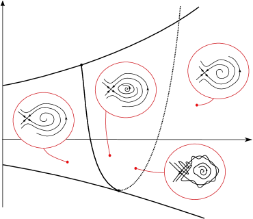
Figure 1. Bifurcation curves for the generalized Hénon map (7) with $R_{n}>0$. The case $R_{n}=0$ corresponds with the bifurcation diagram of the Hénon map. In that case, $L_{n}^{\varphi}$ collapses with $L_{n}$ at $B=1$. The diagram for the case $R_{n}<0$ is similar, changing the position of the curves $L_{n}^{\varphi}$ and $L_{n}$ and the stability of the invariant circle.

The map (7) has in the parameter plane $(M,B)$ the following three bifurcation curves

$$L^{+}_{n}\ :\quad M=-\frac{(1+B)^{2}}{4(1+R_{n})}$$

$$L^{-}_{n}\ :\quad M=\frac{1}{4}(1+B)^{2}(3+R_{n})$$

$$L^{\varphi}_{n}\ :\quad M=\frac{\cos^{2}\omega-\cos\omega(2+R_{n})}{(1+R_{n}/2)^{2}},\quad B=1+\frac{R_{n}\cos\omega}{1+R_{n}/2}.$$

These correspond to the existence of fixed points having multipliers on the unit circle: $+1$ at $(M,B)\in L^{+}_{n}$; $-1$ at $(M,B)\in L^{-}_{n}$; and $e^{\pm i\omega}$ at $(M,B)\in L^{\varphi}_{n}$. Note that the curve $L^{\varphi}_{n}$ is written in a parametric form such that the argument $\omega$ ($0<\omega<\pi$) of the complex multipliers is the parameter. We also point out here the points

$$\mathrm{BT}_{n} :\quad M=\frac{-1-R_{n}}{(1+R_{n}/2)^{2}},\quad B=1+\frac{R_{n}}{1+R_{n}/2}$$ (8)

$$\mathrm{HT}_{n} :\quad M=\frac{3+R_{n}}{(1+R_{n}/2)^{2}},\quad\ \ \ B=\frac{1-R_{n}/2}{1+R_{n}/2}.$$

The are called as follows: Bogdanov-Takens point for $\mathrm{BT}_{n}$ and the Horozov-Takens point for $\mathrm{HT}_{n}$. Also denoted by $L_{n}$ is an interesting curve (nonbifurcational) starting at the point $\mathrm{BT}_{n}$, which corresponds to the existence of a saddle fixed point of (7) of neutral type (i.e., the fixed point has positive multipliers whose product is equal to one). This curve is drawn in Figure 1 as the dotted line and its equation is given by the same expression of $L^{\varphi}_{n}$ replacing $\cos\omega$ by $\alpha>1$.

2pt $K$ at 414 638 $H$ at 310 690 $L_{n}^{-}$ at 120 590 $L^{\varphi}_{n}$ at 230 445 $\mathrm{HT}_{n}$ at 262 575

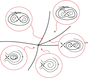
Figure 2. Bifurcation diagrams near a Horozov-Takens point for $R_{n}<0$. For $R_{n}=0$ (Hénon map) the curves $K$ and $H$ collapse at $B=1$. The diagram for the case $R_{n}>0$ is similar but changes the position of $K$, $H$ and the stability of both invariant curves. The open domain between $K$ and $H$ is rather small, having the size of a finite order along the $M$-direction and order $O(R_{n})$ along the $B$-direction.

There is an open domain $D^{s}_{n}$ , bounded by the curves $L^{+}_{n}$, $L^{-}_{n}$ $L^{\varphi}_{n}$ with vertices $\mathrm{BT}_{n}$, $\mathrm{HT}_{n}$ (see Figure 1), such that map (7) has a stable fixed point for parameters in $D^{s}_{n}$. The bifurcations of periodic points with multipliers $e^{\pm i\omega}$ can lead to asymptotically stable or/and unstable invariant circles. The first return map $T_{n}$ has an invariant circle which is either stable if $R_{n}>0$ or unstable if $R_{n}<0$. Observe that the sign of $R_{n}$ actually only depends on $J_{1}\not=0$. Thus, if $J_{1}>0$ we obtain parameter values where we have a stable close invariant curve. In the case $J_{1}<0$, the existence of a stable closed invariant curve in (7) follows from the bifurcation analysis of the Horozov-Takens point $\mathrm{HT}_{n}$. Some of the elements that appear in this non-degenerate bifurcation are showen in Figure 2. Actually, when $J_{1}\not=0$ (i.e, $R_{n}\not=0$), near the point $\mathrm{HT}_{n}$ there are open domains parameter values where stable and unstable closed invariant curves coexist.

Moreover, for any map that is $O(R_{n})$-close to to (7) in the $C^{3}$-topology the corresponding bifurcations still remain non-degenerate and preserve the same stability. Thus, we can obtain the same type of results for the pertubed map (6). To summarize for future reference, for $n$ large enough we find open sets $A^{1}_{n}$, $A^{2}_{n}$ of $(M,B)$-parameters accumulating at $\mathrm{BT}=(-1,1)$ and $\mathrm{HT}=(3,1)$ respectively as $n\to\infty$ such that the following holds. If $(M,B)\in A^{1}_{n}$ (resp. $(M,B)\in A^{2}_{n}$) then $T_{n}$ has a hyperbolic attracting periodic point (resp. a normally hyperbolic attracting invariant circle).

3.2. Proof of Lemma 3.3

By assumption the map $g_{a}$ has a homoclinic tangency at a point $Y_{a}$ associated with a sectional dissipative periodic point $Q_{a}$ for all $a\in a_{0}+(-\alpha,\alpha)^{k}$. Actually, the tangency must be smoothly continued until $\|a-a_{0}\|_{\infty}=\alpha$. We consider a two-parameter unfolding $g_{a,\varepsilon}$ of the homoclinic tangency $Y_{a}$ of $g_{a}$ for $a\in a_{0}+[-\alpha,\alpha]^{k}$, where $\varepsilon=(\mu,\varphi)$. Here $\mu$ is the parameter that controls the splitting of the tangency and $\varphi$ is the perturbation of the argument of the complex eigenvalues of $Q_{a}$. We can take local coordinates $(x,u,y)$ with $x\in\mathbb{C}$, $u\in\mathbb{R}^{m-3}$ and $y\in\mathbb{R}$ in a neighborhood of $Q_{a}$ which corresponds to the origin, such that $W^{s}_{loc}(Q_{a})$ and $W^{u}_{loc}(Q_{a})$ acquire the form $\{y=0\}$ and $\{x=0,u=0\}$ respectively. Moreover, the complex eigenvalues related to the stable manifold of $Q_{a}$ correspond to the $x$-variable and the tangency point $Y_{a}$ is represented by $(x^{+},u^{+},0)$.

Let us consider a $C^{\infty}$-bump function $\phi:\mathbb{R}\to\mathbb{R}$ with support in $[-1,1]$ and equal to 1 on $[-1/2,1/2]$. Let

$$\rho:a=(a_{1},\dots,a_{k})\in\mathbb{I}^{k}\mapsto\phi(a_{1})\cdot\ldots\cdot\phi(a_{k})\in\mathbb{R}.$$

Take $\delta>0$ so that the $\delta$-neighborhoods in local coordinates of $Q_{a}$ and $g_{a}^{-1}(Y_{a})$ are disjoint. Observe that these two neighborhoods, call $U$ and $V$ respectively, can be taken independent of $a$. We can write

$$g_{a,\varepsilon}=H_{a,\varepsilon}\circ g_{a},$$

where $H_{a,{\varepsilon}}$ in these local coordinates takes the form

$$\bar{x} =\left(1-\rho\left(\frac{a-a_{0}}{2\alpha}\right)\phi\left(\frac{\|(x,u,y)\|}{2\delta}\right)(1-e^{i\varphi})\right)x$$

$$\bar{u} =u$$

$$\bar{y} =y+\rho\left(\frac{a-a_{0}}{2\alpha}\right)\phi\left(\frac{\|(x,u,y)-(x^{+},u^{+},0)\|}{2\delta}\right)\mu,$$

and is the identity otherwise. Observe that if $a\not\in a_{0}+(-2\alpha,2\alpha)^{k}$ then $g_{a,\varepsilon}=g_{a}$ and if $(x,u,y)\not\in U\cup V$ then $g_{a,\varepsilon}=g_{a}$.

Recall in Section 3.1 the definition of the first return map associated with the unfolding of a simple homoclinic tangency. Since the tangency point $Y_{a}$ depends $C^{d}$-continuously on $a_{0}+[-\alpha,\alpha]^{k}$, we may assume that the first-return map $T_{n}=T_{n}(a,\varepsilon)$ also depends smoothly as a function of the parameter $a$ on $a_{0}+[-\alpha,\alpha]^{k}$.

Lemma 3.5 (Parametrized rescaling lemma).

There exist families of open sets $(\Delta_{n}(a))_{a}$ of parameters converging to $\varepsilon=0$ as $n\to\infty$ such that for any $\varepsilon\in\Delta_{n}(a)$ the map $T_{n}=T_{n}(a,\varepsilon)$ has an attracting $C^{r}$-manifold $\mathcal{M}_{n}=\mathcal{M}_{n}(a,\varepsilon)$ for any $a\in a_{0}+[-\alpha,\alpha]^{k}$. Moreover, there exists a $C^{d,r}$-family of transformations of coordinates which bring the first-return map $T_{n}$ restricted to $\mathcal{M}_{n}$ to the form given by (6)

$$\bar{x}=y,\qquad\bar{y}=M-Bx-y^{2}-R_{n}(xy+o(1)).$$ (9)

Here the rescaled parameters $M=M_{n}(a,\varepsilon)$ and $B=B_{n}(a,\varepsilon)$ are at least $C^{d}$-smooth functions (recall that $d\leq r-2$) on

$$\Delta_{n}=\left\{(a,\varepsilon):a\in a_{0}+(-\alpha,\alpha)^{k}\ \text{and}\ \varepsilon\in\Delta_{n}(a)\right\}.$$

The same property holds for the coefficient $R_{n}=R_{n}(a,\varepsilon)$ and the $o(1)$-terms. More specifically,

$$M\sim\gamma^{2n}_{a}(\mu+O(\gamma_{a}^{-n}+\lambda_{a}^{n})),\quad B\sim(\lambda_{a}\gamma_{a})^{n}\cos(n\varphi+O(1))\quad\text{and}\quad R_{n}=\frac{2J_{1a}}{B}(\lambda^{2}_{a}\gamma_{a})^{n}$$ (10)

where $\lambda_{a}=\lambda_{a}(g)$ and $\gamma_{a}=\gamma_{a}(g)$ are the eigenvalues of $Q_{a}=Q_{a}(g)$ satisfying (1) for $g_{a}$.

Proof.

Let us analyze the proof of the rescaling lemma in [GST08], more specifically the change of coordinates for the first return maps given in Section 3.2 [GST08] for the case $(2,1)$ with $\lambda\gamma>1$. From equations  [GST08, Eq. (3.12)-(3.16)] we can observe the all the transformations of coordinates can be performed smoothly on the parameter $a\in a_{0}+[-\alpha,\alpha]^{k}$. The exponents that will appear in the orders of convergence will not depend on the parameter $a$ but only on $n$. On the other hand the constants in the $O$-terms will depend on the parameter but these can be uniformely bounded due to the compactness of the parameter space. These considerations allow us basically to apply the rescaling Lemma 3.4 smoothly on the parameter $a\in a_{0}+[-\alpha,\alpha]^{k}$. ∎

Lemma 3.6.

For $n$ large enough, $\Delta_{n}(a)$ can be taken in such a way that

$$\phi_{n,a}:\Delta_{n}(a)\to(-10,10)^{2}\setminus B(0,r),\qquad\phi_{n,a}(\epsilon)=(M_{n}(a,\epsilon),B_{n}(a,\epsilon))$$

is a diffeomorphism where $M_{n}$ and $B_{n}$ are the functions given in (10) for fixed $n$ and $a$. Here $B(0,r)$ is a closed ball of some small fixed radius $r$ around the origin.

Proof.

Let us introduce the parameter value $\varepsilon^{0}_{n}(a)=(\mu_{n}^{0}(a),\varphi^{0}_{n}(a))$, which by definition satisfies $\phi_{n,a}(\varepsilon^{0}_{n}(a))=0$. It can be seen from the expressions of $M$ and $B$ in (10) that $\mu^{0}_{n}(a)=O(\gamma^{-n}_{a}+\lambda^{n}_{a})$ and $\varphi^{0}_{n}(a)=\frac{\pi}{2n}+O(1/n)$. We take out $B(0,r)$ around the origin in $(-10,10)^{2}$ so that $B$ is bounded away from zero and $R_{n}$ is well-defined. Similar values were considered in [GST08, pg. 946] and as is claimed there, the rescaled functions $M$ and $B$ can take arbitrarily finite values when $\mu$ varies close to $\mu^{0}_{n}(a)$ and $\varphi$ near $\varphi^{0}_{n}(a)$. Let us explain this. Although the $O$-functions in (10) depend on $\varepsilon$, the functions $M$ and $B$ basically only depend on $\mu$ and $\varphi$ respectively for $n$ large enough. Actually on [GST08, pg. 946] are giving explicit expressions for $M_{n,a}$ and $B_{n,a}$. Using them one can observe that

$$\partial_{\mu}M_{n,a}\sim\gamma_{a}^{2n}\not=0\quad\text{and}\quad\partial_{\varphi}B_{n,a}\sim n(\lambda_{a}\gamma_{a})^{n}\sin(n\varphi+O(1))\not=0$$

for all $\varepsilon=(\mu,\varphi)$ close to $\varepsilon^{0}_{n}(a)$. Then the Jacobian of $\phi_{n,a}$ converges to infinity, uniformly on $a\in a_{0}+[-\alpha,\alpha]^{k}$ as $n\to\infty$. The rate of growth is exponential. This implies that $\phi_{n,a}$ is an invertible expanding map with arbitrarily large uniform expansion on $a\in a_{0}+[-\alpha,\alpha]^{k}$. On the other hand, the size of $\Delta_{n}(a)$ (coming mainly from considerations on the angle $\varphi$) where the expanding map $\phi_{n,a}$ is defined has decay of order $O(1/n)$. Thus, for $n$ large enough we get that a neighborhood of $\varepsilon^{0}_{n}(a)$ can be taken so that its image under $\phi_{n,a}$ is $(-10,10)^{2}$. In particular we can take $\Delta_{n}(a)$ being diffeomorphic to $(-10,10)^{k}\setminus B(0,r)$. ∎

Consequently,

$$\Phi_{n}(a,\varepsilon)=(a,\phi_{n,a}(\varepsilon))$$

is a diffeomorphism between the set $\Delta_{n}$ defined above and $(a_{0}+[-\alpha,\alpha]^{k})\times(-10,10)^{2}\setminus B(0,r)$. On the other hand, although the coefficient $R_{n}$ depends on $B$, note that the range of values it takes is negligible when $B$ is bounded from zero and $n$ is large enough. Actually from the relations in  (10) it follows that $R_{n}=o(1)$. Thus, the bifurcation diagram of (9) can be studied from the results described in Section 3.1 assuming $R_{n}=o(1)$ independent of $B$.

Let us remind the reader of the Bogdanov-Takens $\mathrm{BT}_{n}(a)$ and the Horozov-Takens $\mathrm{HT}_{n}(a)$ points given in (8), which now also depend on $a$ and accumulate at $\mathrm{BT}=(-1,1)$ and $\mathrm{HT}=(3,1)$ respectively as $n\to\infty$. Hence, according to Section 3.1 for each $n$ large enough we find open subsets $A^{1}_{n}(a)$, $A^{2}_{n}(a)$ in the $(M,B)$-parameter plane such that if $(M,B)\in A^{1}_{n}(a)$ (resp. $(M,B)\in A^{2}_{n}(a)$), then $T_{n}$ has a hyperbolic attracting periodic point (resp.  attracting smooth invariant circle) for all $a\in a_{0}+[-\alpha,\alpha]^{k}$. Moreover, we can assume the points $\mathrm{BT}_{n}(a)$ and $\mathrm{HT}_{n}(a)$ belong to the boundary of $A^{1}_{n}(a)$ and $A^{2}_{n}(a)$ respectively. Since these sets vary $C^{d}$-continuously with respect to the parameter $a\in[-\alpha,\alpha]^{k}$, we can choose $C^{d}$-continuously $(M^{*}_{n}(a),B^{*}_{n}(a))\in A^{*}_{n}(a)$ for $*=1,2$ arbitrarily close to $\mathrm{BT}_{n}(a)$ and $\mathrm{HT}_{n}(a)$ respectively.

Since $\Phi_{n}$ is a diffeomorphism, we may find a $C^{d}$-function $\varepsilon^{*}_{n}(a)=(\mu_{n}^{*}(a),\varphi^{*}_{n}(a))$ for $a\in a_{0}+[-\alpha,\alpha]^{k}$, $*=1,2$, defined as $\Phi_{n}^{-1}(a,(M^{*}_{n}(a),B^{*}_{n}(a))=(a,\varepsilon^{*}_{n}(a))$. In particular,

$$M^{*}_{n}(a) =M_{n,a}(\varepsilon^{*}_{n}(a))\sim\gamma^{2n}_{a}(\mu_{n}^{*}(a)+O(\gamma_{a}^{-n}+\lambda_{a}^{n}))$$ (11)

$$B^{*}_{n}(a) =B_{n,a}(\varepsilon^{*}_{n}(a))\sim(\lambda_{a}\gamma_{a})^{n}\cos(n\varphi^{*}_{n}(a)+O(1)).$$

Extending smoothly $\varepsilon^{*}_{n}(a)$ to $\mathbb{I}^{k}$ we can consider the sequence of families $\tilde{g}_{n}=(\tilde{g}_{n,a})_{a}$ where

$$\tilde{g}_{n,a}=g_{a,\varepsilon^{*}_{n}(a)}\qquad\text{for $a\in\mathbb{I}^{k}$ and $n$ large enough}.$$

Observe that $\tilde{g}_{n,a}=g_{a}$ for $a\not\in a_{0}+(-2\alpha,2\alpha)^{k}$ and we may assume has an $n$-periodic attractor (a sink or an invariant circle) for all $a\in a_{0}+(-\alpha,\alpha)^{k}$.

To conclude the proof of the lemma we only need to show that $\tilde{g}_{n}$ converges to $g$ in the $C^{d,r}$-topology. To do this, notice that the $C^{d,r}$-norm satisfies

$$\|\bar{g}_{n}-g\|=\|(I-H_{a,\varepsilon^{*}_{n}(a)})\circ g_{a}\|\leq\|I-H_{a,\varepsilon^{*}_{n}(a)}\|\,\|g\|$$

where $I$ denotes the identity and the $C^{d,r}$-norm of any $g=(g_{a})_{a}$ in the Berger domain $\mathscr{U}$ is bounded. Thus, we only need to calculate the $C^{d,r}$-norm of the family $(I-H_{a,\varepsilon^{*}_{n}(a)})_{a}$. Since $H_{a,\varepsilon^{*}_{n}(a)}=I$ if $a\not\in a_{0}+(-2\alpha,2\alpha)^{k}$ or $(x,u,y)\not\in U\cup V$, therefore $\|I-H_{a,\varepsilon^{*}_{n}(a)}\|$ is less or equal than

$$\left\|\rho\left(\frac{a-a_{0}}{2\alpha}\right)\phi\left(\frac{\|(x,u,y)\|}{2\delta}\right)(1-e^{i\varphi^{*}_{n}(a)})x\right\|+\left\|\rho\left(\frac{a-a_{0}}{2\alpha}\right)\phi\left(\frac{\|(x,u,y)-(x^{+},u^{+},0)\|}{2\delta}\right)\mu^{*}_{n}(a)\right\|.$$

To estimate the $C^{d,r}$-norms above it suffices to show that the functions

$$F_{n}(a)=\rho(\frac{a-a_{0}}{2\alpha})(1-e^{i\varphi^{*}_{n}(a)})\quad\text{and}\quad G_{n}(a)=\rho(\frac{a-a_{0}}{2\alpha})\mu^{*}_{n}(a)$$

have $C^{d}$-norm small when $n$ is large and $a\in a_{0}+(-2\alpha,2\alpha)^{k}$. Actually we will prove the following:

$$\|F_{n}\|_{C^{d}}=O\left(\frac{\alpha^{-d}}{n}\right)\quad\text{and}\quad\|G_{n}\|_{C^{d}}=O\left(\frac{\alpha^{-d}}{n}\right)$$ (12)

Observe that this assertion completes the proof. To prove this we will need the following derivative estimates on the functions $\mu_{n}^{*}(a)$ and $\varphi_{n}^{*}(a)$. Here the symbol $\partial_{a}^{j}$ is used to denote the $j$-th partial derivative with respect to the coordinates $a_{i}$ of $a$ using the multi-index notation.

Lemma 3.7.

For $1\leq|j|\leq d$

1. $\mu_{n}^{*}(a)=O(\gamma_{a}^{-n}+\lambda_{a}^{n})\ \ \text{and}\ \ \partial_{a}^{j}\mu_{n}^{*}(a)=O(n^{|j|}(\gamma_{a}^{-n}+\lambda_{a}^{n})).$
   

2. $\varphi_{n}^{*}(a)=O\left(\frac{1}{n}\right),\ \ \partial_{a}^{j}\varphi_{n}^{*}(a)=O\left(\frac{n^{{|j|-1}}}{(\gamma_{a}\lambda_{a})^{n}}\right)\ \ \text{and}\ \ \partial_{a}^{j}(e^{i\varphi_{n}^{*}(a)})=O\left(\frac{n^{{|j|-1}}}{(\gamma_{a}\lambda_{a})^{n}}\right).$

Assuming the above lemma let us now prove the estimates in (12), starting with the second one. To do this, using the Leibniz formula,

$$\partial^{\ell}_{a}G_{n}(a)=\sum_{j:j\leq\ell}\binom{\ell}{j}\ \partial_{a}^{\ell-j}\rho\left(\frac{a-a_{0}}{2\alpha}\right)\cdot\partial_{a}^{j}\mu_{n}^{*}(a).$$

Substituting the estimate from Lemma 3.7 (i) in the above expression we obtain that

$$\partial_{a}^{\ell}G_{n,\alpha}(a)=O(\alpha^{-d}\cdot n^{\left|\ell\right|}(\gamma_{a}^{-n}+\lambda_{a}^{n}))$$

which, in fact, implies a better estimate than (12).

To prove the first estimate in (12) for $\|F_{n}\|_{C^{d}}$, using again the Leibniz formula

$$\partial_{a}^{\ell}F_{n,\alpha}(a)=(1-e^{i\varphi_{n}^{*}(a)})\ \partial_{a}^{\ell}\rho\left(\frac{a-a_{0}}{2\alpha}\right)-\sum_{j:\ 0<j\leq\ell}\binom{\ell}{j}\,\ \partial_{a}^{j}(e^{i\varphi_{n}^{*}(a)})\ \partial_{a}^{\ell-j}\rho\left(\frac{a-a_{0}}{2\alpha}\right).$$

Applying Lemma 3.7 (ii),

$$\partial_{a}^{\ell}F_{n,\alpha}(a)=O\left(\frac{\alpha^{-\left|\ell\right|}}{n}\right)+\sum_{j:\ 0<j\leq\ell}\binom{\ell}{j}\,O\left(\frac{n^{{|j|-1}}}{(\gamma_{a}\lambda_{a})^{n}}\cdot\alpha^{-\left|\ell-j\right|}\right).$$

Thus, $\partial_{a}^{\ell}F_{n,\alpha}(a)=O\left(\alpha^{-d}n^{-1}\right)$. To complete the proof of Lemma 3.3 we have to show the estimates of Lemma 3.7.

Proof of Lemma 3.7.

First we will prove the estimates on $\mu_{n}^{*}(a)$ and $\partial_{a}^{j}\mu_{n}^{*}(a)$. Let us first observe that $M$, up to a multiplicative factor, is actually equal to $\gamma^{2n}_{a}(\mu+O(\gamma_{a}^{-n}+\lambda_{a}^{n}))$ (see the exact expressions for $M$ in  [GST08, Section 3.2]). Although this multiplicative factor depends on the perturbation $\varepsilon_{n}$, to avoid notational clutter we will assume in what follows and without loss of generality that this factor is always $1$. Then $M^{*}_{n}(a)$ can be written as

$$M^{*}_{n}(a)=\gamma^{2n}_{a}\mu_{n}^{*}(a)+h_{n}(a)$$ (13)

where $h_{n}(a)$ is independent of $\mu_{n}^{*}(a)$ and $h_{n}(a)=O(\gamma_{a}^{-n}+\lambda_{a}^{n})$. Again using the explicit expressions for $M$ in  [GST08, Section 3.2], one can see that $\partial_{a}^{j}h_{n}(a)=O(n^{|j|}(\gamma_{a}^{-n}+\lambda_{a}^{n}))$.

Claim 3.7.1.

$$M^{*}_{n}=O(1)\quad\text{and}\quad\partial_{a}^{j}M^{*}_{n}=o(1)\ \ \text{for all $1\leq|j|\leq d$}$$ (14)

Proof of Claim 3.7.2.

The expressions of $\mathrm{BT}_{n}(a)$ and $\mathrm{HT}_{n}(a)$ in (8) imply that these functions have order $O(R_{n})$ and analogously their respective derivatives have order $O(\partial_{a}^{j}(R_{n}))$. On the other hand $M^{*}_{n}(a)$ is $O(R_{n})$-close to $\mathrm{BT}_{n}(a)$ or $\mathrm{HT}_{n}(a)$, see Section 3.1. Also the derivatives of $\partial_{a}^{j}M^{*}_{n}$ are $O(\partial_{a}^{j}(R_{n}))$-close. Therefore,

$$M^{*}_{n}=O(1)+O(R_{n})\quad\text{and}\quad\partial_{a}^{j}M^{*}_{n}=O(\partial_{a}^{j}R_{n}).$$

Finally, from the equation for $R_{n}$ given in Lemma 3.5, we have that $R_{n}=o(1)$ and $\partial_{a}^{j}R_{n}=o(1)$. Combining this with the previous estimates proves the claim. ∎

In particular, from (13) we obtain that

$$\gamma^{2n}_{a}\mu_{n}^{*}(a)=O(1)+O(\gamma_{a}^{-n}+\lambda_{a}^{n}),$$

which implies $\mu_{n}^{*}(a)=O(\gamma^{-2n}_{a})=O(\gamma_{a}^{-n}+\lambda_{a}^{n})$. To show the estimates on $\partial_{a}^{j}\mu_{n}^{*}(a)$ we will proceed by an inductive argument on $|j|$. In the case $|j|=1$, taking the derivate of (13) gives

$$\partial_{a}^{j}M^{*}_{n}(a)=\partial_{a}^{j}(\gamma^{2n}_{a})\mu_{n}^{*}(a)+\gamma^{2n}_{a}\partial_{a}^{j}\mu_{n}^{*}(a)+\partial_{a}^{j}h_{n}(a).$$

We have that $\mu_{n}^{*}(a)=O(\gamma_{a}^{-n}+\lambda_{a}^{n})$, $\partial_{a}^{j}M^{*}_{n}(a)=o(1)$ from Claim 3.7.1 and $\partial_{a}^{j}h_{n}(a)=O(n(\gamma_{a}^{n}+\lambda_{a}^{n}))$. Also $\partial_{a}^{j}(\gamma^{2n}_{a})=2n\gamma^{2n-1}_{a}\cdot\partial_{a}^{j}(\gamma_{a})=O(n\gamma^{2n}_{a})$. Combining all these estimates with the previous equation implies

$$\gamma^{2n}_{a}\partial_{a}^{j}\mu_{n}^{*}(a)=O(n\gamma^{2n}_{a})\cdot O(\gamma_{a}^{-n}+\lambda_{a}^{n})+O(n(\gamma_{a}^{-n}+\lambda_{a}^{n}))+o(1).$$

Then $\partial_{a}^{j}\mu_{n}^{*}(a)=O(n(\gamma_{a}^{-n}+\lambda_{a}^{n}))$, which proves the formula for $|j|=1$. To prove the necessary expression for any multi-index $\ell$, we will proceed by induction assuming that $\partial_{a}^{j}\mu_{n}^{*}(a)=O(n^{|j|}(\gamma_{a}^{-n}+\lambda_{a}^{n}))$ for any $j$ with $1\leq|j|<\left|\ell\right|$ and will show the same estimate for $\ell$. From (13) and using the Leibniz formula we obtain

$$\partial_{a}^{\ell}M^{*}_{n}(a)=\sum_{j:j\leq\ell}\binom{\ell}{j}\ \partial_{a}^{\ell-j}(\gamma^{2n}_{a})\cdot\partial_{a}^{j}\mu_{n}^{*}(a)+\partial_{a}^{\ell}h_{n}(a).$$ (15)

Now $\partial_{a}^{\ell-j}(\gamma^{2n}_{a})=O(n^{\left|\ell-j\right|}\gamma^{2n}_{a})$ and so the order of $\partial_{a}^{\ell-j}(\gamma^{2n}_{a})\cdot\partial_{a}^{j}\mu_{n}^{*}(a)$ is

$$O(n^{\left|\ell-j\right|}\gamma^{2n}_{a})\cdot O(n^{|j|}(\gamma_{a}^{-n}+\lambda_{a}^{n}))=O(n^{\left|\ell\right|}\gamma^{2n}_{a}(\gamma_{a}^{-n}+\lambda_{a}^{n})).$$

Also $\partial_{a}^{\ell}M^{*}_{n}(a)=o(1)$ by Claim 3.7.1 and $\partial_{a}^{\ell}h_{n}(a)=O(n^{\left|\ell\right|}(\gamma_{a}^{n}+\lambda_{a}^{n}))$. Then isolating the term with $j=\ell$ from the sum in (15) we get that

$$\gamma^{2n}_{a}\cdot\partial_{a}^{\ell}\mu_{n}^{*}(a)=O(n^{\left|\ell\right|}\gamma^{2n}_{a}(\gamma_{a}^{-n}+\lambda_{a}^{n}))+O(n^{\left|\ell\right|}(\gamma_{a}^{-n}+\lambda_{a}^{n}))+o(1).$$

Then we may conclude that $\partial_{a}^{\ell}\mu_{n}^{*}(a)=O(n^{\left|\ell\right|}(\gamma_{a}^{-n}+\lambda_{a}^{n}))$ proving item (i) of Lemma 3.7.

Now we will prove the second part of the lemma, that is, the estimates on $\varphi_{n}^{*}(a)$ and $\partial_{a}^{j}\varphi_{n}^{*}(a)$. As was mentioned before in Lemma 3.6 because of the expressions in [GST08, pg. 946], we have that $\varphi^{0}_{n}(a)=\frac{\pi}{2n}+O(1/n)$ and the size of $\Delta_{n}(a)$ has decay of order $O(1/n)$. Thus, we may also conclude that $\varphi_{n}^{*}(a)=O(n^{-1})$. Now assuming $\partial_{a}^{j}\varphi_{n}^{*}(a)=O\left(n^{{|j|-1}}(\gamma_{a}\lambda_{a})^{-n}\right)$, it is not hard to see by an inductive argument on the derivatives that also $\partial_{a}^{j}\left(e^{i\varphi_{n}^{*}(a)}\right)=O\left(n^{{|j|-1}}(\gamma_{a}\lambda_{a})^{-n}\right)$.

In what follows we will prove that $\partial_{a}^{j}\varphi_{n}^{*}(a)=O(n^{|j|-1}(\gamma_{a}\lambda_{a})^{-n})$ for $j\geq 1$. This will be done by induction in $|j|$, starting with $|j|=1$. To do this, according to (11) and writting $h_{n}(a)=n\varphi_{n}^{*}(a)+O(1)$, we have that $B^{*}_{n}(a)\sim(\lambda_{a}\gamma_{a})^{n}\cos(h_{n}(a))$. Having in mind the exact expression for the function $B$ given in [GST08, pg. 946], $B_{n}(a)$ differs from $(\lambda_{a}\gamma_{a})^{n}\cos(h_{n}(a))$ by a multiplicative constant $b_{0}$, that depends on $\varepsilon_{n}$. Similarly to what was done for $M^{*}_{n}(a)$ and to avoid unnecessary notational complications we will assume, without loss of generality, that this factor is always $1$. Then,

$$B^{*}_{n}(a)=(\lambda_{a}\gamma_{a})^{n}\cos(h_{n}(a))$$ (16)

and derivating both sides of the equation with respect to some index $j$, $|j|=1$, we obtain

$$\partial_{a}^{j}B^{*}_{n}(a) =n\cdot B^{*}_{n}(a)\cdot\partial_{a}^{j}(\log\lambda_{a}\gamma_{a})+(\lambda_{a}\gamma_{a})^{n}\sin(h_{n}(a))\cdot\partial_{a}^{j}h_{n}(a).$$ (17)

Now to estimate the order of $\partial_{a}^{j}B^{*}_{n}(a)$, we have the following claim whose proof we omit as it is analogous to that of Claim 3.7.1.

Claim 3.7.2.

$$B^{*}_{n}=O(1)\quad\text{and}\quad\partial_{a}^{j}B^{*}_{n}=o(1)\ \ \text{for all $1\leq|j|\leq d$}$$ (18)

Since the norms of the functions $B^{*}_{n}(a),\ \partial_{a}^{j}(\log\lambda_{a}\gamma_{a})$ are bounded from above and using that $\partial_{a}^{j}B^{*}_{n}=o(1)$ due to Claim 3.7.2 we get from (17) that

$$(\lambda_{a}\gamma_{a})^{n}\sin(h_{n}(a))\cdot\partial_{a}^{j}h_{n}(a)=O(n)+o(1).$$ (19)

Since $\sin(h_{n}(a))$ is bounded away from zero by the choice of $\varphi_{n}$, resolving the previous equation for $\partial_{a}^{j}h_{n}(a)$ we obtain that $\partial_{a}^{j}h_{n}(a)=O(n(\lambda_{a}\gamma_{a})^{-n})$. This implies that $\partial_{a}^{j}\varphi_{n}^{*}(a)=O((\lambda_{a}\gamma_{a})^{-n})$ and proves the formula for $|j|=1$. To prove the expression for any index $\ell$, we will proceed by induction assuming that $\partial_{a}^{j}h_{n}(a)=O(n^{|j|}(\gamma_{a}\lambda_{a})^{-n})$ for any $j$ with $1\leq|j|<\left|\ell\right|$ and will show that $\partial_{a}^{\ell}h_{n}(a)=O(n^{\left|\ell\right|}(\gamma_{a}\lambda_{a})^{-n})$. This will imply that $\partial_{a}^{\ell}\varphi_{n}^{*}(a)=O(n^{\left|\ell\right|-1}(\lambda_{a}\gamma_{a})^{-n})$, as it is required to complete the proof of the lemma.

Take $\ell$ with $\left|\ell\right|>1$, and fix $\iota<\ell$ such that $\left|\iota\right|=1$. Since $\partial_{a}^{\ell}B^{*}_{n}(a)=\partial_{a}^{\ell-\iota}(\partial_{a}^{\iota}B^{*}_{n}(a))$ we get from (16), (17) and by using the Leibniz formula,

$$\partial_{a}^{\ell}B^{*}_{n}(a)=n\cdot\partial_{a}^{\ell-\iota}(B^{*}_{n}(a)\cdot\partial_{a}(\log\lambda_{a}\gamma_{a}))+\sum_{j:j\leq(\ell-\iota)}\binom{\ell-\iota}{j}\,\partial_{a}^{(\ell-\iota)-j}((\lambda_{a}\gamma_{a})^{n}\sin(h_{n}(a)))\cdot\partial_{a}^{j+\iota}h_{n}(a).$$ (20)

Now we will determine the order of the terms in the above equation.

Claim 3.7.3.

$$\partial_{a}^{j}((\lambda_{a}\gamma_{a})^{n}\sin(h_{n}(a)))=O(n^{|j|}(\lambda_{a}\gamma_{a})^{n})\quad\text{for all $1\leq|j|\leq d$}$$ (21)

Proof of Claim 3.7.3.

Observe from (16) that $[(\lambda_{a}\gamma_{a})^{n}\sin(h_{n}(a))]^{2}=(\lambda_{a}\gamma_{a})^{2n}-(B^{*}_{n})^{2}$. Since $\partial_{a}^{j}B^{*}_{n}=o(1)$ from Claim 3.7.2, we get that

$$\partial_{a}^{j}((\lambda_{a}\gamma_{a})^{n}\sin(h_{n}(a)))=O(\partial_{a}^{j}(\lambda_{a}\gamma_{a})^{n}).$$

On the other hand it can be seen by an inductive argument that $\partial_{a}^{j}(\lambda_{a}\gamma_{a})^{n}=O(n^{|j|}(\lambda_{a}\gamma_{a})^{n})$, which gives the required estimate. ∎

For $j<(\ell-\iota)$, by the induction hypothesis $\partial_{a}^{j+\iota}h_{n}(a)=O(n^{\left|j+\iota\right|}(\gamma_{a}\lambda_{a})^{-n})$. Combining this with Claim 3.7.3 we obtain that for $j<(\ell-\iota)$

$$\partial_{a}^{(\ell-\iota)-j}((\lambda_{a}\gamma_{a})^{n}\sin(h_{n}(a)))\cdot\partial_{a}^{j+\iota}h_{n}(a)=O(n^{\left|(\ell-\iota)-j\right|}(\lambda_{a}\gamma_{a})^{n})\cdot O(n^{\left|j+\iota\right|}(\gamma_{a}\lambda_{a})^{-n})=O(n^{\ell}).$$

On the other hand $\partial_{a}^{\ell}B^{*}_{n}(a)=o(1)$ and $n\cdot\partial_{a}^{\ell-\iota}(B^{*}_{n}(a)\cdot\partial_{a}(\log\lambda_{a}\gamma_{a}))=O(n)$. Thus, putting all these estimates together in (20) and isolating the term corresponding with the index $j=\ell-\iota$ we obtain

$$(\lambda_{a}\gamma_{a})^{n}\sin(h_{n}(a)))\cdot\partial_{a}^{\ell}h_{n}(a)=O(n)+O(n^{\left|\ell\right|})+o(1).$$

This implies that $\partial_{a}^{\ell}h_{n}(a)=O(n^{\left|\ell\right|}(\gamma_{a}\lambda_{a})^{-n})$ concluding the proof. ∎

References

- [BD12] C. Bonatti and L. J. Díaz. Abundance of -homoclinic tangencies. Transactions of the American Mathematical Society, 264:5111–5148, 2012.
- [Ber16] P. Berger. Generic family with robustly infinitely many sinks. Inventiones mathematicae, 205(1):121–172, 2016.
- [Ber17] P. Berger. Emergence and non-typicality of the finiteness of the attractors in many topologies. Proceedings of the Steklov Institute of Mathematics, 297(1):1–27, May 2017.
- [BR21] P. G. Barrientos and A. Raibekas. Robust degenerated unfoldings of cycles and tangencies. Journal Dynamics Differential Equations, 33:177–209, 2021.
- [Col98] E. Colli. Infinitely many coexisting strange attractors. Annales de l’Institut Henri Poincare-Nonlinear Analysis, 15(5):539–580, 1998.
- [GG00] S. Gonchenko and V. Gonchenko. On Andronov-Hopf bifurcations of two-dimensional diffeomorphisms with homoclinic tangencies, 2000.
- [GG04] S. V. Gonchenko and V. Gonchenko. On bifurcations of birth of closed invariant curves in the case of two-dimensional diffeomorphisms with homoclinic tangencies. Trudy Matematicheskogo Instituta imeni VA Steklova, 244:87–114, 2004.
- [GGT07] S. Gonchenko, V. Gonchenko, and J. Tatjer. Bifurcations of three-dimensional diffeomorphisms with non-simple quadratic homoclinic tangencies and generalized Hénon maps. Regular and Chaotic Dynamics, 12(3):233–266, 2007.
- [GKM05] V. Gonchenko, Y. A. Kuznetsov, and H. G. Meijer. Generalized Hénon map and bifurcations of homoclinic tangencies. SIAM Journal on Applied Dynamical Systems, 4(2):407–436, 2005.
- [GST08] S. V. Gonchenko, L. P. Shilnikov, and D. V. Turaev. On dynamical properties of multidimensional diffeomorphisms from Newhouse regions: I. Nonlinearity, 21(5):923, 2008.
- [GTS93] S. Gonchenko, D. Turaev, and L. Shilnikov. On an existence of newhouse regions near systems with non-rough poincaré homoclinic curve (multidimensional case). Doklady Akademii Nauk, 329(4):404–407, 1993.
- [HK10] B. R. Hunt and V. Y. Kaloshin. Prevalence. In Handbook of dynamical systems, volume 3, pages 43–87. Elsevier, 2010.
- [KS17] S. Kiriki and T. Soma. Takens’ last problem and existence of non-trivial wandering domains. Advances in Mathematics, 306:524–588, 2017.
- [Lea08] B. Leal. High dimension diffeomorphisms exhibiting infinitely many strange attractors. Annales de l’Institut Henri Poincare (C) Non Linear Analysis, 25(3):587–607, 2008.
- [New74] S. E. Newhouse. Diffeomorphisms with infinitely many sinks. Topology, 13:9–18, 1974.
- [New79] S. E. Newhouse. The abundance of wild hyperbolic sets and nonsmooth stable sets for diffeomorphisms. Inst. Hautes Études Sci. Publ. Math., 50:101–151, 1979.
- [PT93] J. Palis and F. Takens. Hyperbolicity and sensitive chaotic dynamics at homoclinic bifurcations, volume 35 of Cambridge Studies in Advanced Mathematics. Cambridge University Press, Cambridge, 1993. Fractal dimensions and infinitely many attractors.
- [PV94] J. Palis and M. Viana. High dimension diffeomorphisms displaying infinitely many periodic attractors. Ann. of Math. (2), 140(1):207–250, 1994.
- [Rob83] C. Robinson. Bifurcation to infinitely many sinks. Communications in Mathematical Physics, 90(3):433–459, 1983.
- [Rom95] N. Romero. Persistence of homoclinic tangencies in higher dimensions. Ergodic Theory Dynam. Systems, 15(4):735–757, 1995.
- [Tri14] M. Triestino. Généricité au sens probabiliste dans les difféomorphismes du cercle. Ensaios Matemáticos, 27:1–98, 2014.